CASSOWARY 20: a Wide Separation Einstein Cross Identified with the X-shooter Spectrograph

Abstract

We have used spectra obtained with X-shooter, the triple arm optical-infrared spectrograph recently commissioned on the Very Large Telescope (VLT) of the European Southern Observatory (ESO), to confirm the gravitational lens nature of the CASSOWARY candidate CSWA 20. This system consists of a luminous red galaxy at redshift $z_{\rm abs}=0.741$, with a very high velocity dispersion, $\sigma_{\rm lens}\simeq 500$ km s^-1, which lenses a blue star-forming galaxy at $z_{\rm em}=1.433$ into four images with mean separation of $\sim 6^{\prime\prime}$. The source shares many of its properties with those of UV-selected galaxies at $z=2$–3: it is forming stars at a rate $\textrm{SFR}\simeq 25M_{\odot}$ yr^-1, has a metallicity of $\sim 1/4$ solar, and shows nebular emission from two components separated by $0.4^{\prime\prime}$ (in the image plane), possibly indicating a merger. It appears that foreground interstellar material within the galaxy has been evacuated from the sight-line along which we observe the starburst, giving an unextinguished view of its stars and H ii regions. CSWA 20, with its massive lensing galaxy producing a high magnification of an intrinsically luminous background galaxy, is a promising target for future studies at a variety of wavelengths.

1 Introduction

The large cosmic volume surveyed by the Sloan Digital Sky Survey (SDSS) has sparked, among many other projects, several systematic searches for strong gravitational lens systems (Bolton et al. 2006; Willis et al. 2006; Estrada et al. 2007; Ofek et al. 2008; Shin et al. 2008; Belokurov et al. 2009; Kubo et al. 2009; Lin et al. 2009; Wen et al. 2009). All of these studies share the dual motivation of, on the one hand, probing the high-mass end of the galaxy mass function and the underlying distribution of dark matter in the lensing galaxies and, on the other, identifying highly magnified high redshift sources. The latter can bring within reach of current astronomical instrumentation detailed studies of stellar populations and interstellar gas at high redshifts which would otherwise have to wait until the advent of the next generation of 30+ m optical-infrared telescopes (e.g. Pettini et al. 2000, 2002; Teplitz et al. 2000; Lemoine-Busserolle et al. 2003; Smail et al. 2007; Cabanac, Valls-Gabaud, & Lidman 2008; Siana et al. 2008, 2009; Finkelstein et al. 2009; Hainline et al. 2009; Quider et al. 2009, 2010; Yuan & Kewley 2009 and references therein).

Table 1: SDSS Positions and Magnitudes of Components of CSWA 20 Lens System

Image	RA (J2000)	Dec (J2000)	$u$	$g$	$r$	$i$	$z$
Lens	14 41 49.16	+14 41 20.6	$24.6\pm 1.1$	$25.1\pm 0.5$	$22.7\pm 0.2$	$20.70\pm 0.06$	$20.2\pm 0.2$
i1	14 41 49.38	+14 41 21.3	$21.46\pm 0.15$	$21.60\pm 0.05$	$21.54\pm 0.07$	$21.87\pm 0.17$	$21.76\pm 0.63$
i2	14 41 49.24	+14 41 22.8	$21.89\pm 0.26$	$21.65\pm 0.06$	$21.40\pm 0.08$	$21.27\pm 0.13$	$21.89\pm 0.88$
i3	14 41 48.93	+14 41 22.2	$21.56\pm 0.23$	$21.52\pm 0.07$	$21.46\pm 0.11$	$21.27\pm 0.16$	$21.18\pm 0.67$
i4	14 41 49.18	+14 41 18.7	$21.58\pm 0.23$	$21.57\pm 0.07$	$21.16\pm 0.08$	$21.19\pm 0.16$	$20.59\pm 0.38$

Note: Positional errors are $\leq 0.1^{\prime\prime}$ for images i1–i4, and $\simeq 0.1^{\prime\prime}$ for the lensing galaxy.

The CAmbridge Sloan Survey Of Wide ARcs in the skY (CASSOWARY) targets multiple, blue companions around massive ellipticals in the SDSS photometric catalogue as likely candidates for wide-separation gravitational lens systems. A comprehensive description of the search strategy is given by Belokurov et al. (2009). Of the twenty highest priority CASSOWARY candidates, eight have so far been confirmed as gravitational lenses and the redshifts of both lens and source measured—see http://www.ast.cam.ac.uk/research/cassowary/ for further details.

In this paper, we report observations of a ninth system, CASSOWARY 20 or CSWA 20 for short. As can be seen from Figure 1, CSWA 20 consists of four blue images around a red galaxy, in a configuration reminiscent of the Einstein Cross (Adam et al. 1989), but with a factor of $\sim 3$ larger separation between the images. The observations reported here, obtained during the commissioning of the triple arm spectrograph X-shooter on the VLT, confirm the gravitational lens nature of the system by showing that three of the four blue images are of the same source, a star-forming galaxy at redshift $z_{\rm em}=1.433$, and that the lens is a massive elliptical galaxy at $z_{\rm abs}=0.741$ (the fourth blue image was not observed, but is most likely to be a fourth gravitationally lensed image of the $z=1.433$ galaxy). Table LABEL:tab:sdss_photom gives positions and magnitudes for the different components of the system. The four images of the source are all of similar magnitudes (e.g. $g=21.52$–21.65) and all have very blue colours, with $-0.14\leq(u-g)\leq+0.24$ and $+0.06\leq(g-r)\leq+0.41$. In contrast, the lens has red colours with $(g-r)=+2.4$ and $(r-i)=+2.0$.

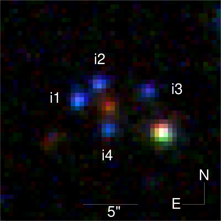
Figure 1: Colour-composite ($g,r,i$) SDSS image of the CSWA 20 lens system. Positions and magnitudes of the different components are listed in Table LABEL:tab:sdss_photom.

In Section 2, we give a concise description of the X-shooter instrument and details of the observations and data reduction. Section 3 describes a simple lensing model we have applied to CSWA 20, while Sections 4 and 5 present our measurements of the spectra of the lens and source respectively. We summarise our results in Section 6. Throughout this paper we use a ‘737’ cosmology with $H_{0}=70$ km s^-1 Mpc^-1, $\Omega_{\rm M}=0.3$ and $\Omega_{\Lambda}=0.7$.

2 Observations and Data Reduction

Table 2: Details of X-shooter Observations of CSWA 20

Date (UT)	Exp. Time (s)	Slit PA (∘)	Comments
2009 March 19	$2\times 1500$ (UV-B, VIS-R)	117	Two exposures on targets, nodded.
	$2\times 1600$ (NIR)		Slit across i1 and i2 (see Figure 1).
2009 May 05	$4\times 1500$ (UV-B, VIS-R, NIR)	11	Two exposures on targets, two on sky.
			Slit across i2, lensing galaxy, and marginally i4.

2.1 X-shooter

X-shooter is the first of the second generation VLT instruments to be made available to the ESO community; it was built by a consortium of institutes in Denmark, France, Italy and the Netherlands, in collaboration with ESO which was responsible for the final integration and installation on the VLT. A full description of the instrument is provided by D’Odorico et al. (2006). X-shooter consists of three echelle spectrographs with prism cross-dispersion, mounted on a common structure at the Cassegrain focus of the Unit Telescope 2 (Kueyen). The light beam from the telescope is split in the instrument by two dichroics which direct the light in the spectral ranges 300–550 nm and 550-1015 nm to the slits of the UV-B and VIS-R spectrographs respectively. The undeviated beam feeds the NIR spectrograph with wavelengths in the range 1025–2400 nm. The UV-B and VIS-R spectrographs operate at ambient temperature and pressure and deliver two-dimensional spectra on the $2048\times 4102$ 15 $\mu$m pixel E2V CCD and $2048\times 4096$, 15 $\mu$m pixel MIT/LL CCD respectively. The NIR spectrograph is enclosed in a vacuum vessel and kept at a temperature of approximately 80 K by a continuous flow of liquid nitrogen. The NIR detector is a Teledyne substrate-removed HgCdTe Hawaii-2RG array, with $2048\times 2048$ 18 $\mu$m pixels. The spectral format in the three spectrographs is fixed; the final spectral resolution is determined by the choice of slit width with each spectrograph having its own slit selection device.

2.2 Observations

After two commissioning runs with the UV-B and VIS-R spectrographs in November 2008 and January 2009, the instrument was operated in its full three-arm configuration in two further commissioning runs in March 2009 and May 2009 during which the observations of CSWA 20 were obtained. This lens candidate was selected as a good test of the instrument performance for faint galaxy studies. Different observation strategies were attempted, as detailed in Table LABEL:tab:obs. In March 2009 the $11^{\prime\prime}$ long entrance slit was rotated to a position angle on the sky PA $=117^{\circ}$ and positioned so as to record simultaneously the spectra of images i1 and i2 (see Figure 1). In May 2009 the slit was placed across image i2 and the lensing galaxy (PA $=11^{\circ}$); this set-up also captured some of the light from image i4. For all observations the slit widths were 1^′′ (UV-B), 0.9^′′ (VIS-R), and 0.9^′′ (NIR); the corresponding resolving powers are $R\equiv\lambda/\Delta\lambda=5100$, 8800, and 5600, sampled with 3.2, 3.0, and 4.0 wavelength bins respectively (after on-chip binning by a factor of two of the UV-B and VIS-R detectors). The observations used a nodding along the slit approach, with an offset of $4^{\prime\prime}$ between individual exposures. All calibration frames needed for data processing were obtained on the day after the observations.

2.3 Data Reduction

The spectra were processed with a preliminary version of the X-shooter data reduction pipeline (Goldoni et al. 2006). Pixels in the two-dimensional (2D) frames are first mapped to wavelength space using calibration frames. Sky emission lines are subtracted before any resampling using the method developed by Kelson (2003). The different orders are then extracted, rectified, wavelength calibrated and merged, with a weighted average used in the overlapping regions. The final product is a one dimensional, background-subtracted spectrum and the corresponding error file. Intermediate products including the sky spectrum and individual echelle orders are also available. We followed all of these steps, although we used standard iraf tools for extracting the 1D spectra (using a predefined aperture) while this aspect of the pipeline data processing was being refined.

The VIS-R and NIR spectra were corrected for telluric absorption by dividing their spectra by that of the O8.5 star Hip 69892, observed with the same instrumental set-up and at approximately the same airmass as CSWA 20. Absolute flux calibration used as reference the Hubble Space Telescope white dwarf standard GD 71 (Bohlin et al. 2001) whose spectrum was recorded during the same nights as CSWA 20.

3 Lensing Models

As discussed in detail in Sections 4 and 5, the X-shooter spectra show the lens to be an absorption line galaxy at $z_{\rm abs}=0.741$, and three of the four blue images (i1, i2, and i4) to be those of an emission line galaxy at $z_{\rm em}=1.433$. With the assumption that i3 is also a gravitationally lensed image of the same galaxy, we can use these redhifts together with the data in Table LABEL:tab:sdss_photom to develop some simple lensing models for CSWA 20. The aims are to obtain estimates of the enclosed mass within the images and hence the velocity dispersion of the lensing galaxy, as well as estimates of the total magnification of the images.

Before formal modelling, let us begin with a very simple model to estimate rough, order of magnitude effects. Suppose the lens is an isolated singular isothermal sphere with a constant velocity dispersion $\sigma$. The lensing properties of this model are discussed by Schneider, Ehlers & Falco (1992), who show that the typical deflection is:

$$\Delta\theta=1\aas@@fstack{\prime\prime}15\left({\sigma_{v}\over 200{\rm\,km\,s}^{-1}}\right)^{2}\left({D_{\rm ds}\over D_{\rm s}}\right)$$ (1)

where $D_{\rm ds}$ is the angular diameter distance between deflector and source, whilst $D_{\rm s}$ is the distance between observer and source. A simple estimate of the velocity dispersion can be immediately obtained by requiring that the isothermal sphere deflection given by eq.(1) reproduce the observed deflections ($\Delta\theta\sim 3^{\prime\prime}$) for the distances $D_{\rm ds}$ and $D_{\rm s}$ implied by the values of $z_{\rm abs}$ and $z_{\rm em}$ in our cosmology. This already suggests that the lensing galaxy is very massive with $\sigma\sim 500$ km s^-1.

Of course, mass distributions in nature are not spherically symmetric. Ellipticity occurs both because of the intrinsic flattening of the lens galaxy and because of the external tidal shear generated by neighbouring galaxies. We therefore wish to supplement our simple model with more realistic, flattened mass distributions. These can reproduce not just the separations, but also the detailed positions of all four putative images.

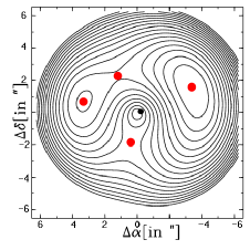
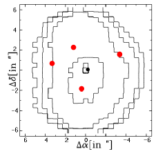
Figure 2: A PixeLens model of CSWA 20 with image locations (red dots) and source locations (black dots). The left panels shows the Fermat surface, from which the parity of the images can be inferred. The right panel shows the pixellated mass distribution in units of the critical surface mass density.

A powerful way of modelling gravitational lenses is to pixellate the projected mass distribution of the lensing galaxies into tiles. Mass can be apportioned to each tile. The mass on the tiles is unknown, but fixed by requiring that the mass distribution reproduce the images with the observed parities and locations. Of course the problem is then under-determined, as there are many more unknowns than constraints, but can be regularised by requiring that the mass distribution is isothermal-like. This simple idea has been developed by Williams & Saha (2004) into the PixeLens code, which provides flattened generalisations of the isothermal sphere.

In detail, the solution space for the masses on the tiles is sampled using a Markov chain Monte Carlo method. We typically generate an ensemble of 1000 models that reproduce the input data, which in our case are the image locations given in Table LABEL:tab:sdss_photom. As the constraint equations are linear, averaging the ensemble also produces a solution, which is displayed in Figure 2.

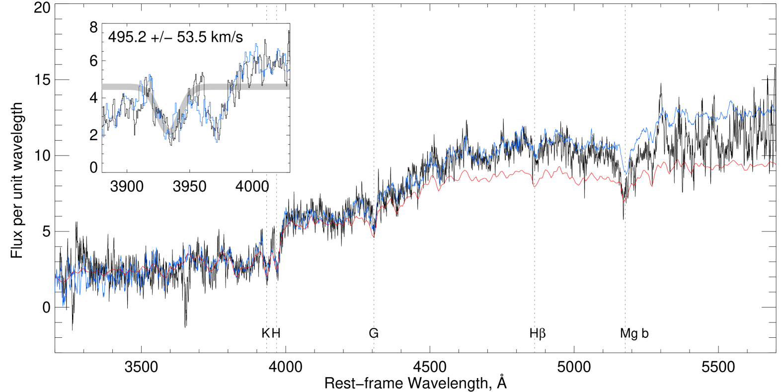
Figure 3: Three spectra are shown in this Figure. Black: Portion of the X-shooter spectrum of the lensing galaxy in CSWA 20, boxcar smoothed with a three-pixel wide filter. Blue: The spectrum of SDSS J010354.1+144814.1 the galaxy with the largest velocity dispersion ($\sigma=530\pm 60$ km s^-1) in the sample of Bernardi et al. (2006). Red: Model spectrum of a 12 Gyr old single burst of star formation, from Maraston et al. (2009). The inset shows a detailed view of the spectral region encompassing the Ca ii H & K lines, together with our Gaussian fit.

The left panel shows the arrival time surface. The images lie at the stationary points of the surface and are marked with red dots. In the model, we see that the images i1 and i3 correspond to local minima and so are positive parity, whereas i2 and i4 correspond to saddles and so are negative parity. The model predicts an additional, de-magnified central image which – as is customary – is too faint for detection. The right panel shows the contours of projected mass of the absorption line galaxy (in terms of the critical surface mass density). This is mildly elliptical in the inner parts, and falls off in an isothermal-like manner.

From the PixeLens model, we compute the (cylindrical) mass within the Einstein radius (21.1 kpc) as $M=(4.4\pm 0.4)\times 10^{12}M_{\odot}$. This implies a velocity dispersion for the lensing galaxy of $530\pm 20$ km s^-1, if it is isothermal. As we shall see in Section 4, such a high velocity dispersion is consistent with the widths of the absorption lines in the X-shooter spectrum of the lens. The errors have been calculated using PixeLens to generate 1000 models that reproduce the input data. From these distributions, we calculate the error on the enclosed mass by constructing 68 per cent confidence limits. The error on the enclosed mass gives an error on the velocity dispersion via the Jeans equations. The total magnification is rather poorly constrained with the present data, but most of the models have a total magnification (for the four images) of factors between $\sim 3$ and $\sim 6$

4 The Lens: a Massive Galaxy at $z_{\rm abs}=0.741$

The spectrum of the deflector galaxy, reproduced in Figure 3, shows the signatures of an old stellar population at a redshift $z_{\rm abs}=0.741$. The galaxy has a prominent 4000 Å break, and strong Ca ii H & K, G-band and Mg$b$ $\lambda\lambda 5167.3,5172.7,5183.6$ absorption features. H$\beta$ absorption is also present. The signal-to-noise ratio of the data is only modest, but Gaussian fits to the Ca ii H&K absorption (see inset in Figure 3) result in an estimate of the velocity dispersion $\sigma=495\pm 54$ km s^-1 after correcting for instrumental broadening (which is minimal, since $\sigma_{\rm instr}\simeq 15$ km s^-1). Additional observations with higher signal-to-noise ratio are required to provide a significantly improved measure of the velocity dispersion. The overall spectral energy distribution at optical wavelengths is similar to those of luminous red galaxies (LRGs) at lower redshifts, as can be appreciated from the comparison in Figure 3 with the SDSS spectrum of J010354.1+144814.1, the most massive galaxy found by Bernardi et al. (2006) with no obvious indication that its large velocity dispersion ($\sigma=530\pm 60$ km s^-1) may be due to the superposition of two objects along the line of sight. Also shown in Figure 3 is the model spectrum computed by Maraston et al. (2009) for a 12 Gyr old single burst of star formation with solar metallicity; this comparison further illustrates the very red continuum (longward of the G-band) of the deflector galaxy in CSWA 20.

Given the relatively high redshift, and associated $(1+z)^{4}$ surface brightness dimming, it is not surprising that the galaxy is barely detected in the SDSS $r$-band image and that the $i$-band magnitude is poorly determined. Only the core of the galaxy is evident in the SDSS images, with an apparent effective radius of $<3$ kpc, and deeper, higher-resolution imaging is needed to determine its structural properties. However, we can put some constraints on its total luminosity from the X-shooter spectral data. The integrals of the deflector’s spectral energy distribution multiplied by the SDSS $r$-band and $i$-band response curves give $r=21.7$ and $i=20.1$ respectively. Given the slit width of $0.9^{\prime\prime}$, a mean seeing of FWHM $=0.65^{\prime\prime}$, and assuming an effective radius of the galaxy $r_{\rm e}=10$ kpc (typical of LRGs, Bernardi et al. 2008) which corresponds to $r_{\rm e}=1.1^{\prime\prime}$ at $z=0.741$, we calculate that $\sim 40$% of the total galaxy light falls within the X-shooter slit. The estimate of the $i$-band magnitude is then $i=19.1$. Adopting a $k$-correction of $-1.0$ mag, an evolutionary correction of 0.8 mag and rest-frame colour $(r-i)=0.4$ (appropriate to a 12 Gyr old passively evolving Maraston et al. 2009 model), then gives a corrected $r=18.9$, and a corresponding absolute magnitude of $M_{\rm r}=-24.4$. With these parameters, this galaxy is among the most massive and luminous red galaxies known (Bernardi et al. 2006).

5 The Source: a Luminous Star-Forming Galaxy at $z_{\rm em}=1.433$

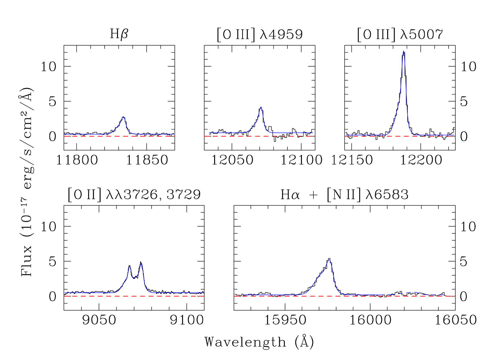
Figure 4: A selection of nebular emission lines in the CSWA 20 lensed galaxy. In each panel, the black histogram shows the data, while the blue continuous line is the fit with the parameters given in Table 4.

As mentioned in Section 2.2, our observations of the source in CSWA 20 cover images i1 and i2 (the latter observed at two epochs—see Table LABEL:tab:obs). In order to improve the signal-to-noise ratio (S/N), we added together the spectra of i1 and i2 (after converting the wavelengths to a vacuum heliocentric frame of reference and binning to a common wavelength grid) and used this composite spectrum in the analysis described below. The spectrum shows a number of narrow emission lines superposed on a weak blue continuum (see Figure 4); the line identifications in Table 3 indicate a redshift $z_{\rm em}=1.433$.

We also recorded image i4 on the second observing run on 2009 May 05, but the slit position, chosen to cover image i2 and the Lens, only captured a small fraction of the light of i4. While this spectrum does show the strongest emission lines at a similar redshift as i1 and i2 (with small differences attributable to the fact that the image of i4 was offset relative to the slit centre, leading to an offset in the wavelength calibration), it was not included in the composite because its S/N is much lower than that of i1 and i2.

5.1 Nebular Emission Lines

From the lensing model described in Section 3, it was concluded that the overall magnification factor for the four images of the Einstein cross is between  $\sim 3$ and $\sim 6$. It can also be seen from Table LABEL:tab:sdss_photom that in the $u$ and $g$ filters images i1 and i2 account for approximately half of the total flux, that is $u$(i1+i2) $\simeq u$(i3+i4), and similarly for the $g$ magnitudes. Thus, in all the following analysis we shall assume, for simplicity, that a magnification factor of $\sim 5/2=2.5$ applies to the quantities measured for i1+i2.

With this assumption and the knowledge of the redshift, we can immediately estimate the luminosity of the source, and compare it with that of other galaxies at similar redshifts. Luminosity functions at $z\lower 2.15277pt\hbox{$\;\buildrel>\over{\sim}\;$}2$ have been measured mostly in the rest-frame far-UV continuum, at 1700 Å (e.g. Reddy et al. 2008). At a redshift $z=1.433$, this corresponds to an observed wavelength of 4136 Å, which falls between the transmission of the SDSS $u$ and $g$ filters. From Table LABEL:tab:sdss_photom we find that $u{\rm(i1+i2)}=20.9$ and $g{\rm(i1+i2)}=20.87$. Adopting a magnitude $m_{\rm 1700}{\rm(i1+i2)}=20.9+2.5\log(1+z)=21.9$ (on the AB scale), we deduce that at $z=1.433$ this corresponds to an absolute magnitude $M_{\rm 1700}{\rm(i1+i2)}=-23.2$. Correcting for the magnification by a factor of 2.5, we find that the source luminosity at 1700 Å is $L_{\rm 1700}\simeq 6L^{\ast}$, compared to $L_{\rm 1700}^{\ast}=-20.3$ obtained by interpolating between the luminosity functions of star-forming galaxies at $z=1$ and 2 (Reddy & Steidel 2009).

Such a high luminosity may indicate that our lensing model underestimates the magnification of the source. However, we also note that in the typical $z\sim 2$ galaxy (equivalent data are not yet available for galaxies at $z\simeq 1.5$) the UV continuum at 1700 Å is dimmed by a factor of $\sim 4-5$ by dust absorption (Reddy & Steidel 2004; Reddy et al. 2006; Erb et al. 2006c). As we shall see below, the source in CSWA 20 is unusual in showing no evidence for dust absorption. Thus, its high UV luminosity may well be the result of unusually low reddening, rather than an exceptionally large number of OB stars.

At $z=1.433$ our data cover the rest-frame wavelength interval from $\sim 1350$ Å to $\sim 9050$ Å. Table 3 lists the emission lines identified in the composite X-shooter spectrum of images i1 and i2 of CSWA 20; the most prominent of these are reproduced in Figure 4. The presence of a number of other spectral features can be surmised from the data, although their S/N is too low (with the relatively short integration time devoted to this object during instrument commissioning) to warrant their measurement. Among these, we recognise the P Cygni profile of C iv $\lambda 1549.1$ due to massive stars, which is a common feature of the integrated spectra of star-forming galaxies (e.g. Schwartz et al. 2006; Quider et al. 2010).

As can be realised from inspection of Figure 4, the line profiles are asymmetric with an extended blue wing, suggesting that they consist of more than one component. Inspection of the 2D images confirms the presence of two components, separated by $\sim 0.4^{\prime\prime}$ along the slit and by $\sim 100$ km s^-1 in the spectral direction. It is possible that the source consists of two merging clumps of gas and stars. In future, it should be possible with better data to extract these two components separately and compare their properties. Given the limited S/N ratio of the current observations, we opted for a single extraction (Section 2.3) which blends together the light from the two clumps, and results in the asymmetric line profiles evident in Figure 4. When these emission lines are analysed with Gaussian fitting routines, as explained below, they appear to consist of two components with the parameters listed in Table 4. However, it is important to keep in mind that these parameters refer to the blend of the emission lines from the two clumps, and may well turn out to be different from the individual values appropriate to each clump when the two are analysed separately. However, the total flux values deduced for the emission lines and listed in Table 3 should not be affected.

Thus, in order to deduce redshifts $z_{\rm em}$, velocity dispersions $\sigma$, and line fluxes $F$, we fitted the emission lines with two Gaussian components, using ELF (Emission Line Fitting) routines in the Starlink dipso data analysis package (Howarth et al. 2004), as well as custom-built software. The fitting proceeded as follows.

Table 3: Emission Lines identified in Images i1 and i2 of CSWA 20

Line	$\lambda_{\rm lab}^{\rm a}$ (Å)	$F^{\rm b}$	Comments
[N ii]	6585.27	$\leq 0.45$	This line is undetected
H$\alpha$	6564.614	$4.9\pm 0.1$	Affected by sky residuals
[O iii]	5008.239	$7.0\pm 0.1$
[O iii]	4960.295	$2.23\pm 0.07$
H$\beta$	4862.721	$1.65\pm 0.04$
[O ii]	3729.86	$2.09\pm 0.03$	Blended with [O ii] $\lambda 3727$
[O ii]	3727.10	$1.56\pm 0.03$	Blended with [O ii] $\lambda 3729$
Mg ii	2803.5324	$0.27\pm 0.05$
Mg ii	2796.3553	$0.48\pm 0.06$
C iii]	1908.734	($0.18$)c	Noisy
[C  iii]	1906.683	($0.25$)c	Noisy

^a Vacuum wavelengths.

^b Integrated line flux in units of 10^-16 erg s^-1 cm^-2.

^c Uncertain measurement.

The best observed emission lines among those listed in Table 3 are the [O iii] doublet and H$\beta$, as they are relatively strong and free from sky residuals. Consequently, we first fitted these three nebular lines, using custom-built Gaussian fitting routines which allowed the redshift, velocity dispersion, and flux in each component to vary but with the constraint that the redshift and velocity dispersion of each component should be the same for all three lines, and therefore using the data from all three lines to find the values of $z_{\rm em}$ and $\sigma$ which minimise the difference between computed and observed profiles. Errors on the values of $z_{\rm em}$, $\sigma$, and $F$ so deduced were estimated using a Monte Carlo approach, whereby the best fitting computed profile was perturbed with a random realisation of the error spectrum and refitted. The process was repeated 100 times and the error in each quantity ($\delta z_{\rm em}$, $\delta\sigma$, $\delta F$) taken to be the standard deviation of the values generated by the 100 Monte Carlo runs.

Table 4 lists the values of $z_{\rm em}$, and $\sigma$ so derived (after subtracting in quadrature the value of $\sigma_{\rm INSTR}$ corresponding to the instrumental resolution of the appropriate X-shooter spectrum—see Section 2.2). The theoretical profiles computed with the parameters in Table 4 and the line fluxes in Table 3 are shown with continuous lines in Figure 4.

In the next stage of the process we applied the values of $z_{\rm em}$ and $\sigma$ deduced from the analysis of the [O iii] and H$\beta$ lines to the [O ii] doublet which is only partially resolved, leaving the flux in each member of the doublet as the only free parameter. As can be seen from Figure 4, the model parameters in Table 4 provide a satisfactory fit to the [O ii] doublet. The fit to H$\alpha$ seemingly required a small shift in the redshift of the narrower component, corresponding to a velocity difference $\Delta v=+25$ km s^-1, or $\sim 2$ wavelength bins, but we suspect that this is an artifact of sky residuals which affect the H$\alpha$ emission line more than other spectral features. The integrated flux in the line is the same independently of whether this shift is applied or not.

The measurements collected in Tables 3 and 4 allow us to determine a range of physical properties for the lensed galaxy in CSWR 20. Before discussing the more involved derivations, we point out two straightforward conclusions. First, we note that the ratio F(H$\alpha$)/F(H$\beta)=2.95\pm 0.1$ is as expected from Case B recombination, F(H$\alpha$)/F(H$\beta)=2.86$ (Brocklehurst 1971), with the ‘standard’ parameters of temperature $T=10\,000$ K and electron density $n(e)=100$ cm^-3 (the density dependence is in any case minimal, and the temperature dependence is minor). Thus it appears that the emission line gas is essentially unreddened. A lack of dust in this galaxy (as viewed from Earth) is further indicated by the blue UV continuum: the photometry in Table LABEL:tab:sdss_photom implies a UV spectrum which is flat in $f_{\rm\nu}$, as expected for an unreddened population of OB stars (e.g. Bruzual & Charlot 2003).

Second, the [O ii] doublet ratio, which is sensitive to density (Osterbrock 1989), is found to be close to the low density limit: $F(3729)/F(3727)=1.33$ implies $n(e)=110$ cm^-3. While at face value the ratio of the [C iii] doublet lines would suggest much higher electron densities ($>1000$ cm^-3), these lines are considerably weaker than [O ii] and their ratio is much more uncertain, so that we consider the value of $n(e)$ deduced from [O ii] to be the more reliable.

Table 4: Profile Decomposition of [O iii] and H$\beta$ Emission Lines

Component	$z_{\rm em}$	$\sigma^{\rm a}$ (km s-1)
1	$1.43308\pm 0.00004$	$85\pm 3$
2	$1.43354\pm 0.00001$	$26\pm 3$

^a Corrected for the instrumental resolution.

5.2 Star-Formation Rate

The H$\beta$ flux given in Table 3 implies a luminosity $L({\rm H}\beta)=2.1\times 10^{42}$ erg s^-1 in our cosmology. Adopting the Case B recombination ratio, F(H$\alpha$)/F(H$\beta)=2.86$, the corresponding H$\alpha$ luminosity is $L({\rm H}\alpha)=6.0\times 10^{42}$ erg s^-1, which in turn implies a star formation rate:

$${\rm SFR}=7.9\times 10^{-42}L({\rm H}\alpha)\cdot\frac{1}{1.8}\cdot\frac{1}{2.5}\cdot 2=21(M_{\odot}\,{\rm yr}^{-1})~{}.$$ (2)

The first term on the right-hand side of eq. (2) is the conversion factor between $L$(H$\alpha$) and SFR proposed by Kennicutt (1998), to which we apply three corrections, as follows. The first adjustment, by the factor of 1/1.8, takes into account the flattening of the stellar initial mass function (IMF) for masses below $1M_{\odot}$ (Chabrier 2003) compared to the single power law of the Salpeter IMF assumed by Kennicutt (1998). The second correction factor is the $2.5\times$ magnification we estimated for the sum of images i1 and i2 (Section 3). The last term corrects for light loss through the spectrograph slit, which we estimate to be a factor of $\sim 2$ by comparing the measured UV flux in the X-shooter spectrum with the SDSS magnitudes given in Table LABEL:tab:sdss_photom. A factor of $\sim 2$ slit loss is typical of near-IR observations of nebular emission lines from high-$z$ galaxies (e.g. Erb et al. 2006c).

An independent measure of the SFR is provided by the UV continuum from OB stars. From $u{\rm(i1+i2)}=g{\rm(i1+i2)}=20.9$ (Table LABEL:tab:sdss_photom), we have $f_{\nu}(1700)=1.6\times 10^{-28}$ erg s^-1 cm^-2 Hz^-1 from the definition of AB magnitudes in terms of $f_{\nu}$. The corresponding luminosity $L_{\nu}(1700)=8.3\times 10^{29}$ erg s^-1 Hz^-1 in turn implies:

$${\rm SFR}=1.4\times 10^{-28}L_{\nu}(1700)\cdot\frac{1}{1.8}\cdot\frac{1}{2.5}=26(M_{\odot}\,{\rm yr}^{-1})~{},$$ (3)

using Kennicutt’s (1998) scaling between $L_{\rm UV}$ and SFR and applying the same corrections as above for the Chabrier (2003) IMF and magnification factor. The good agreement between the SFR estimates from the UV continuum and the Balmer lines is a further indication that the OB stars and H ii regions of this galaxy suffer very little reddening from dust.

5.3 Metallicity

Since we detect emission lines of [O ii], [O iii], and H$\beta$, we can use the $R_{23}\equiv[F(3726)+F(3729)+F(4959)+F(5007)]/F({\rm H}\beta)$ index first proposed by Pagel et al. (1979) as an approximate measure of the oxygen abundance in the absence of direct temperature diagnostics. Over the thirty years since the seminal paper by Pagel and collaborators, many studies have shown that the values of (O/H) so deduced are accurate to within a factor of $\sim 2$ when applied to the integrated spectra of galaxies (e.g. Pettini 2006; Kewley & Ellison 2008 and references therein).

Figure 5 shows the dependence of (O/H) on $R_{23}$ using the analytical expressions by McGaugh (1991) as given by Kobulnicky et al. (1999); these formulae express O/H in terms of $R_{23}$ and the ionization index O${}_{32}\equiv[F(4959)+F(5007)]/[F(3726)+F(3729)]$. The double-valued nature of the $R_{23}$ index translates to an uncertainty in the oxygen abundance between $12+{\rm(O/H)}=8.09$ and 8.52, or between $\sim 1/4$ and $\sim 3/4$ of the solar abundance $12+{\rm(O/H)}_{\odot}=8.69$ (Asplund et al. 2009).

The degeneracy can be broken by considering the [N ii]/H$\alpha$ ratio. According to Pettini & Pagel (2004), our upper limit on the $N2\equiv\log[F(6583)/F(H\alpha)]$ index, $N2\leq-1.04$ (Table 3), implies $12+{\rm(O/H)}\leq 8.26$, or $\leq 2/5{\rm(O/H)}_{\odot}$, favouring the lower branch solution of the $R_{23}$ method. A metallicity of $\sim 1/4$ solar is not unusual for star-forming galaxies at $z=2$–3 (Erb et al. 2006a; Maiolino et al. 2008).

     

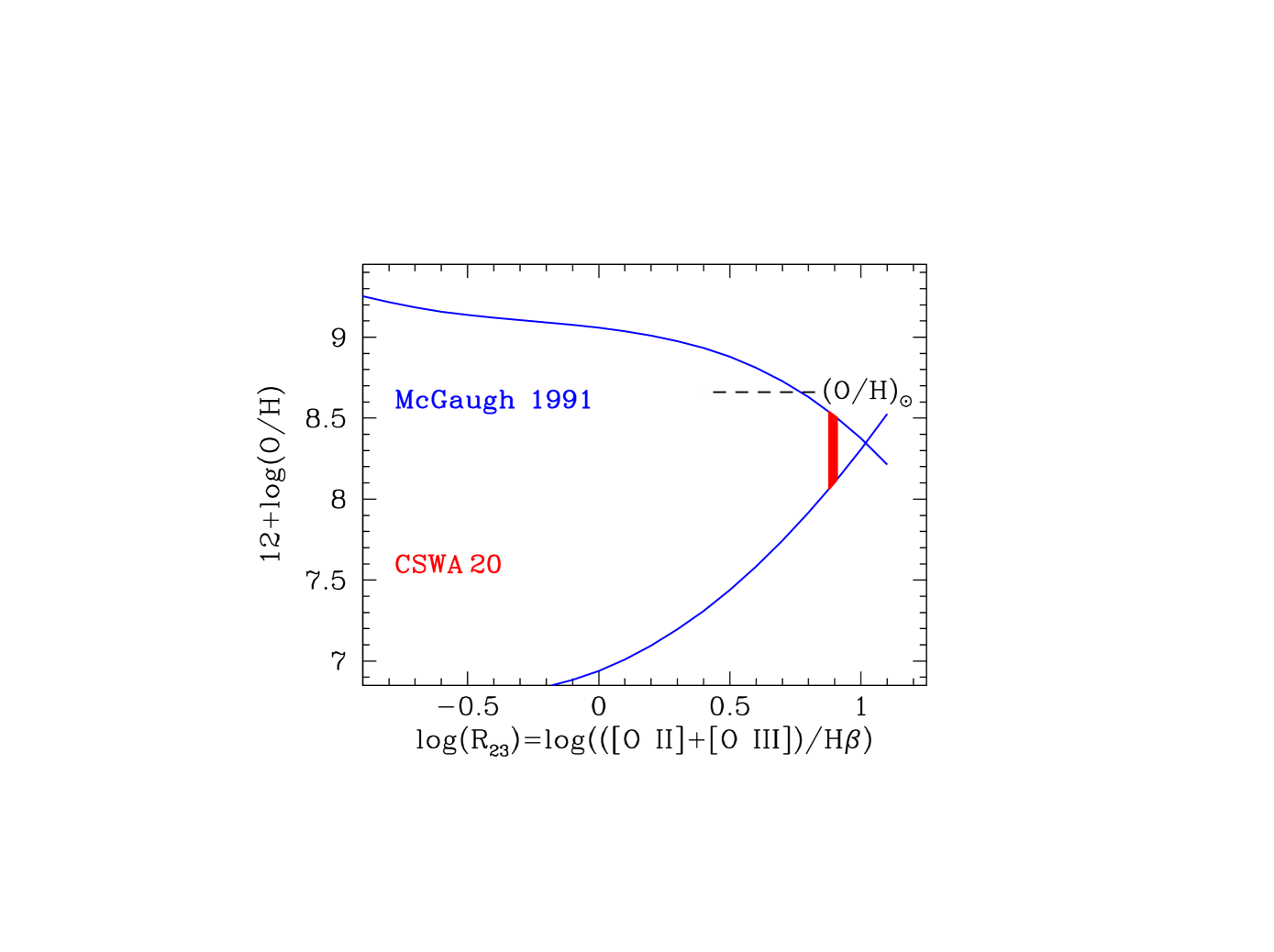
Figure 5: Oxygen abundance from the $R_{\rm 23}$ index. The continuous lines are the calibration byMcGaugh (1991) for the measured ionization index $O_{\rm 32}=$ [O iii]/[O ii], while the shaded area shows the values allowed by the measured $R_{\rm 23}$ line ratio and its statistical $1\sigma$ error. The broken horizontal line is the reference solar oxygen abundance $12+\log{\rm(O/H)}=8.69$ (Asplund et al. 2009).

5.4 Mg ii Emission

We conclude this Section by commenting briefly on the presence of narrow Mg ii $\lambda\lambda 2796,2803$ lines among the nebular emission seen in CSWA 20. These lines are weak (see Figure 6), although undoubtedly real ($8\sigma$ and $5\sigma$ detections respectively—see Table 3). To our knowledge, narrow Mg ii emission has rarely been reported in nearby extragalactic H ii regions, but this could be due to the fact that this wavelength region has not been observed extensively in extragalactic nebulae and, if the two lines are generally weak, existing observations may not have the sensitivity and resolution to detect them.

Broad Mg ii emission is of course a common feature in the spectra of Active Galactic Nuclei (AGN), but we find no evidence in our spectrum of CSWA 20 for the presence of an AGN. Specifically: (a) the Mg ii lines are narrow (the profile decomposition into two Gaussians returns values of $\sigma$ comparable to those listed in Table 4); (b) we detect no high ionisation emission lines due to an AGN in the rest-frame spectral range 1350–9050 Å of our data; and (c) the nebular emission line ratios fall well away from the locus occupied by AGN in diagnostic diagrams such as that shown in Figure 7.

It is possible that in star-forming galaxies at intermediate redshifts weak Mg ii emission is more common than anticipated. In their survey of 1406 galaxies at $z\sim 1.4$, Weiner et al. (2009) identified a small proportion of galaxies (50/1406, or $\approx 3.5$%) with ‘excess’ Mg ii emission whose nature they were unable to establish with certainty. However, even their stacked spectrum of the remaining 1356 galaxies does show weak Mg ii P Cygni profiles, with broad blueshifted absorption and weak emission redshifted by a few 10s of km s^-1. Galaxies with ‘excess’ emission tend to be bluer than average.

CSWA 20 appears to fit into this general pattern, with the exception that no strong absorption component is evident. Thus, it is possible that the unusual lack of absorbing material in front of the stars and H ii regions suggested by the negligible reddening noted above gives an unimpeded view of the intrinsic Mg ii emission from the H ii regions of this galaxy. It is interesting that, when fitted with two Gaussian components, as described in Section 5.1 for the other nebular lines, the best fitting values of redshift for the two components in Mg ii differ by $\Delta v=+30$ km s^-1 ($\sim 3$ wavelength bins) from the corresponding values listed in Table 4. We do not believe that this difference is due to an incorrect wavelength calibration, because we checked the accuracy of the wavelength scale in this region of the spectrum by reference to sky emission lines, and found it to be $\pm 2$ km s^-1 ($\sim 1/5$ of a wavelength bin). If the shift to longer wavelengths is not due to noise, it may be an indication of radiation transfer effects in an expanding medium, analogous to those commonly seen in the Lyman $\alpha$ line (e.g. Verhamme, Schaerer, & Maselli 2006; Steidel et al. 2010).

          

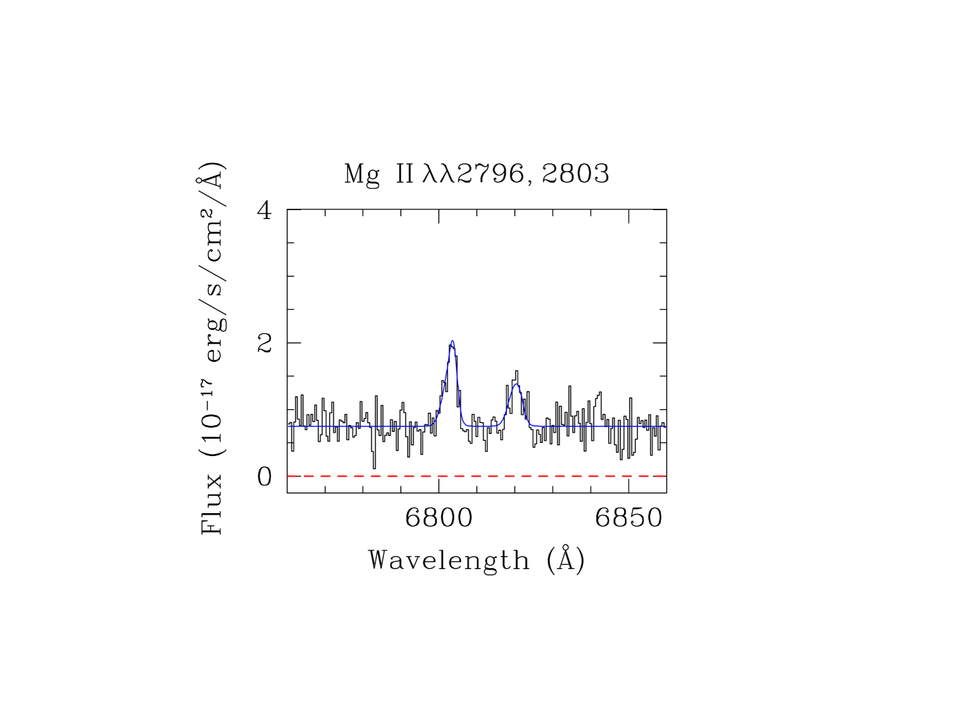
Figure 6: Mg ii $\lambda\lambda 2796,2803$ emission lines in the CSWA 20 lensed galaxy. The black histogram shows the data, while the blue continuous line is our two component Gaussian fit (see text for further details).

   

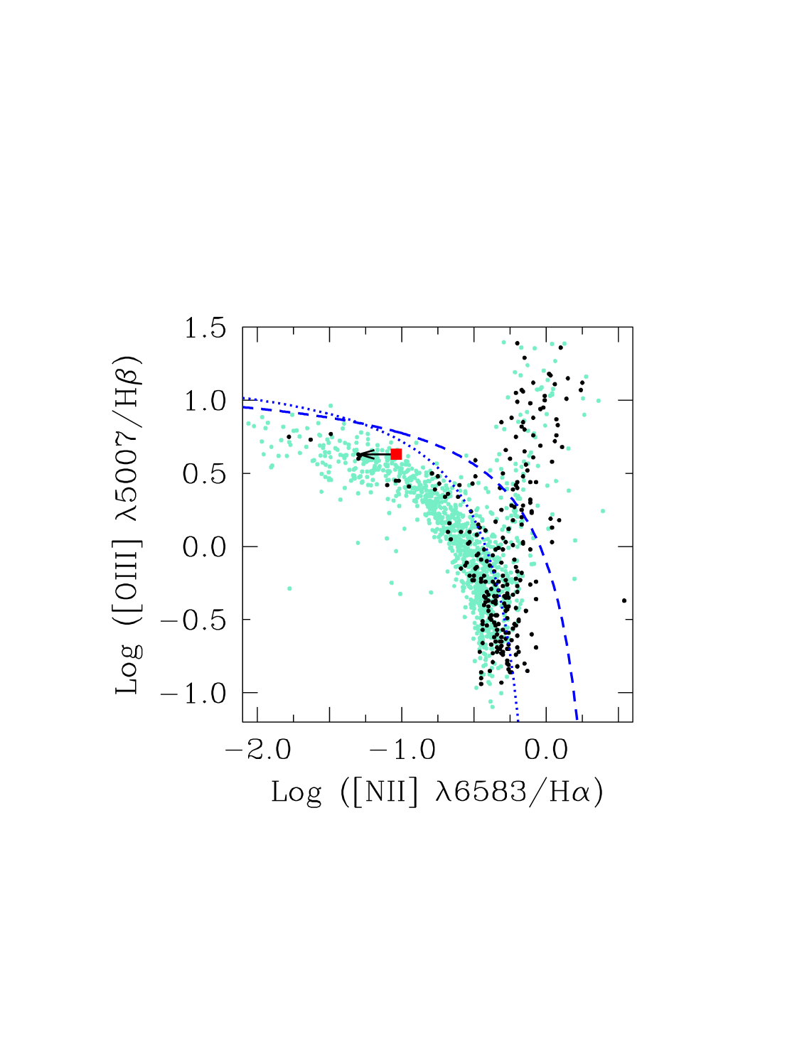
Figure 7: [O iii]/H$\beta$ vs. [N ii]/H$\alpha$ diagnostic diagram. The location of the lensed galaxy in CSWA 20 is shown by the red square and left-pointing arrow. The small green circles are galaxies from the KISS survey (Salzer et al. 2005) and the small black dots are local starburst galaxies from Kewley et al. (2001). The dashed line shows the locus of points which Kewley et al. (2001) consider to be the theoretical limit for starbursts, in the sense that galaxies without an AGN component should fall below and to the left of this line. The dotted line is an empirical determination by Kauffmann et al. (2003) of the same limit. The presence of an AGN in CSWA 20 seems unlikely, given the weakness of the [N ii] emission.

6 Summary and Conclusions

We have presented X-shooter observations, which are among the first obtained with this new VLT instrument, confirming the gravitational lens nature of CSWA 20. This system, originally identified as a candidate from the CASSOWARY search of SDSS images, is found to consist of a luminous red galaxy at $z_{\rm abs}=0.741$ which magnifies the light from a background star-forming galaxy at $z_{\rm em}=1.433$ into four images of approximately equal brightness. With a velocity dispersion $\sigma_{\rm lens}\simeq 500$ km s^-1, the lensing galaxy is among the most massive known; the mass $M\sim 4\times 10^{12}M_{\odot}$ enclosed within the Einstein radius ($\sim 21$ kpc) is responsible for the wide separations ($\simeq 6^{\prime\prime}$) between the four gravitationally lensed images of the source.

The source blue colours satisfy the ‘BM’ photometric selection criteria of Steidel et al. (2004), which isolate galaxies in the redshift interval $1.4\lower 2.15277pt\hbox{$\;\buildrel<\over{\sim}\;$}z\lower 2.15277pt\hbox{$\;\buildrel<\over{\sim}\;$}2.0$. BM galaxies have been relatively little studied up to now. The source in CSWA 20 shares many of the properties of the much better characterised sample of ‘BX’ galaxies at $z\simeq 2$. Its star-formation rate, $\textrm{SFR}\simeq 25M_{\odot}$ yr^-1, metallicity $\textrm{(O/H)}\simeq 0.25\,\textrm{(O/H)}_{\odot}$, and velocity dispersion (equivalent to two components separated by $\Delta v=57$ km s^-1, with $\sigma_{1}=85$ km s^-1 and $\sigma_{2}=26$ km s^-1), are all within the range of values appropriate to star-forming galaxies at $z=2$–3. The galaxy in CSWA 20 is, however, unusual in its low degree of reddening; only $\sim 5$% of the BX galaxies studied by Erb et al. (2006b) have values of $E(B-V)\simeq 0$, as found for this source. Evidently, we view the starburst from a direction along which most of the foreground interstellar material in the galaxy has been evacuated. The lack of dust extinction probably contributes to the unusually high UV luminosity of this galaxy, $L_{1700\,\AA}\sim 6L^{\ast}_{1700\,\AA}$, and the absence of absorbing gas in front of the H ii regions may be the reason why we can detect weak Mg ii resonance lines in emission.

The observations presented here are a good demonstration of the new opportunities for studies of high-$z$ galaxies afforded by the availability of X-shooter. Data secured with less than two hours of integration on two of the four images (with magnitudes $g\simeq r\simeq 21.5$) have been sufficient to characterise many of the salient properties of both lens and source, thanks to the high efficiency and wide wavelength coverage of this unique instrument. Longer observations, achieving higher S/N ratios, will in future shed further light on the nature of both the massive foreground LRG and the background star-forming galaxy. The gravitational magnification will make it possible to study the internal structure of the latter on unusually small scales, by comparing the individual spectra of the four images (e.g. Stark et al. 2008). With more strongly-lensed systems continuing to be found, the characteristics of X-shooter will veritably open a new window on the high-redshift universe, well ahead of the era of 30+ m telescopes.

References

- Adam et al. (1989) Adam, G., Bacon, R., Courtes, G., Georgelin, Y., Monnet, G., & Pecontal, E. 1989, A&A, 208, L15
- (2) Asplund, M., Grevesse, N., Sauval, A. J., & Scott, P. 2009, ARA&A, 47, 481
- Belokurov et al. (2007) Belokurov, V., et al. 2007, ApJL, 671, L9
- Belokurov et al. (2009) Belokurov, V., Evans, N. W., Hewett, P. C., Moiseev, A., McMahon, R. G., Sanchez, S. F., & King, L. J. 2009, MNRAS, 392, 104
- Bernardi et al. (2006) Bernardi M., et al., 2006, AJ, 131, 2018
- Bernardi et al. (2008) Bernardi, M., Hyde, J. B., Fritz, A., Sheth, R. K., Gebhardt, K., & Nichol, R. C. 2008, MNRAS, 391, 1191
- Bohlin et al. (1995) Bohlin, R. C., Colina, L., & Finley, D. S. 1995, AJ, 110, 1316
- Bohlin et al. (2001) Bohlin, R. C., Dickinson, M. E., & Calzetti, D. 2001, AJ, 122, 2118
- Bolton et al. (2006) Bolton, A. S., Burles, S., Koopmans, L. V. E., Treu, T., & Moustakas, L. A. 2006, ApJ, 638, 703
- Brocklehurst (1971) Brocklehurst, M. 1971, MNRAS, 153, 471
- Bruzual & Charlot (2003) Bruzual, G., & Charlot, S. 2003, MNRAS, 344, 1000
- Cabanac et al. (2008) Cabanac, R. A., Valls-Gabaud, D., & Lidman, C. 2008, MNRAS, 386, 2065
- Chabrier (2003) Chabrier, G. 2003, PASP, 115, 763
- D’Odorico et al. (2006) D’Odorico, S., et al. 2006, Proc. SPIE, 6269, 626933
- Erb et al. (2006a) Erb, D. K., Shapley, A. E., Pettini, M., Steidel, C. C., Reddy, N. A., & Adelberger, K. L. 2006a, ApJ, 644, 813
- Erb et al. (2006b) Erb, D. K., Steidel, C. C., Shapley, A. E., Pettini, M., Reddy, N. A., & Adelberger, K. L. 2006b, ApJ, 646, 107
- Erb et al. (2006c) Erb, D. K., Steidel, C. C., Shapley, A. E., Pettini, M., Reddy, N. A., & Adelberger, K. L. 2006c, ApJ, 647, 128
- Estrada et al. (2007) Estrada, J., et al. 2007, ApJ, 660, 1176
- Finkelstein et al. (2009) Finkelstein, S. L., Papovich, C., Rudnick, G., Egami, E., LeFloc’h, E., Rieke, M. J., Rigby, J. R., & Willmer, C. N. A. 2009, ApJ, 700, 376
- Goldoni et al. (2006) Goldoni, P., Royer, F., François, P., Horrobin, M., Blanc, G., Vernet, J., Modigliani, A., & Larsen, J. 2006, Proc. SPIE, 6269, 62692K
- Hainline et al. (2009) Hainline, K. N., Shapley, A. E., Kornei, K. A., Pettini, M., Buckley-Geer, E., Allam, S. S., & Tucker, D. L. 2009, ApJ, 701, 52
- Howarth et al. (2004) Howarth, I. D., Murray, J., Mills, D., & Berry, D. S. 2004, in Starlink User Note 50.24, (Swindon: PPARC), http://www.starlink.rl.ac.uk/star/docs/sun50.htx/sun50.html
- Kauffmann et al. (2003) Kauffmann, G., et al. 2003, MNRAS, 346, 1055
- Kelson (2003) Kelson, D. D. 2003, PASP, 115, 688
- Kennicutt (1998) Kennicutt, R. C., Jr. 1998, ARA&A, 36, 189
- Kewley et al. (2001) Kewley, L. J., Dopita, M. A., Sutherland, R. S., Heisler, C. A., & Trevena, J. 2001, ApJ, 556, 121
- Kewley & Ellison (2008) Kewley, L. J., & Ellison, S. L. 2008, ApJ, 681, 1183
- Kobulnicky et al. (1999) Kobulnicky, H. A., Kennicutt, R. C., Jr., & Pizagno, J. L. 1999, ApJ, 514, 544
- Kubo et al. (2009) Kubo, J. M., Allam, S. S., Annis, J., Buckley-Geer, E. J., Diehl, H. T., Kubik, D., Lin, H., & Tucker, D. 2009, ApJL, 696, L61
- Lemoine-Busserolle et al. (2003) Lemoine-Busserolle, M., Contini, T., Pelló, R., Le Borgne, J.-F., Kneib, J.-P., & Lidman, C. 2003, A&A, 397, 839
- Lin et al. (2009) Lin, H., et al. 2009, ApJ, 699, 1242
- Maiolino et al. (2008) Maiolino, R., et al. 2008, A&A, 488, 463
- Maraston et al. (2009) Maraston C., Strömbäck G., Thomas D., Wake D. A., Nichol R. C., 2009, MNRAS, 394, L107
- McGaugh (1991) McGaugh, S. S. 1991, ApJ, 380, 140
- Ofek et al. (2008) Ofek, E. O., Seitz, S., & Klein, F. 2008, MNRAS, 389, 311
- Osterbrock (1989) Osterbrock, D. E. 1989, Astrophysics of gaseous nebulae and active galactic nuclei, University Science Books.
- Pagel et al. (1979) Pagel, B. E. J., Edmunds, M. G., Blackwell, D. E., Chun, M. S., & Smith, G. 1979, MNRAS, 189, 95
- (38) Pettini, M. 2006 in LeBrun V., Mazure A., Arnouts S. & Burgarella D., eds., The Fabulous Destiny of Galaxies: Bridging Past and Present. Frontier Group, Paris, p. 319 (astro-ph/0603066).
- Pettini & Pagel (2004) Pettini, M., & Pagel, B. E. J. 2004, MNRAS, 348, L59
- Pettini et al. (2002) Pettini, M., Rix, S. A., Steidel, C. C., Adelberger, K. L., Hunt, M. P., & Shapley, A. E. 2002, ApJ, 569, 742
- Pettini et al. (2001) Pettini, M., Shapley, A. E., Steidel, C. C., Cuby, J.-G., Dickinson, M., Moorwood, A. F. M., Adelberger, K. L., & Giavalisco, M. 2001, ApJ, 554, 981
- Pettini et al. (2000) Pettini, M., Steidel, C. C., Adelberger, K. L., Dickinson, M., & Giavalisco, M. 2000, ApJ, 528, 96
- Quider et al. (2009) Quider, A. M., Pettini, M., Shapley, A. E., & Steidel, C. C. 2009, MNRAS, 398, 1263
- Quider et al. (2010) Quider, A. M., Pettini, M., Shapley, A. E., Steidel, C. C., & Stark, D. P. 2010, MNRAS, in press
- Reddy & Steidel (2004) Reddy, N. A., & Steidel, C. C. 2004, ApJL, 603, L13
- Reddy & Steidel (2009) Reddy, N. A., & Steidel, C. C. 2009, ApJ, 692, 778
- Reddy et al. (2006) Reddy, N. A., Steidel, C. C., Fadda, D., Yan, L., Pettini, M., Shapley, A. E., Erb, D. K., & Adelberger, K. L. 2006, ApJ, 644, 792
- Reddy et al. (2008) Reddy, N. A., Steidel, C. C., Pettini, M., Adelberger, K. L., Shapley, A. E., Erb, D. K., & Dickinson, M. 2008, ApJS, 175, 48
- Saha & Williams (2004) Saha, P., Williams, L. L. R. 2004, AJ, 127, 2604
- Salzer et al. (2005) Salzer, J. J., Jangren, A., Gronwall, C., Werk, J. K., Chomiuk, L. B., Caperton, K. A., Melbourne, J., & McKinstry, K. 2005, AJ, 130, 2584
- Schlegel et al. (1998) Schlegel, D. J., Finkbeiner, D. P., & Davis, M. 1998, ApJ, 500, 525
- Schneider, Ehlers & Falco (1992) Schneider, P., Ehlers, J., Falco, E.E. 1992. Gravitational Lenses, Springer Verlag, Berlin.
- Schwartz et al. (2006) Schwartz, C. M., Martin, C. L., Chandar, R., Leitherer, C., Heckman, T. M., & Oey, M. S. 2006, ApJ, 646, 858
- Shin et al. (2008) Shin, M.-S., Strauss, M. A., Oguri, M., Inada, N., Falco, E. E., Broadhurst, T., & Gunn, J. E. 2008, AJ, 136, 44
- Siana et al. (2009) Siana, B., et al. 2009, ApJ, 698, 1273
- Siana et al. (2008) Siana, B., Teplitz, H. I., Chary, R.-R., Colbert, J., & Frayer, D. T. 2008, ApJ, 689, 59
- Smail et al. (2007) Smail, I., et al. 2007, ApJL, 654, L33
- Steidel et al. (2010) Steidel, C. C., Erb, D. K., Shapley, A. E., Pettini, M., Reddy, N. A., & Bogosavljevic, M. 2010, ApJ, submitted.
- Steidel et al. (2004) Steidel, C. C., Shapley, A. E., Pettini, M., Adelberger, K. L., Erb, D. K., Reddy, N. A., & Hunt, M. P. 2004, ApJ, 604, 534
- Stark et al. (2008) Stark, D. P., Swinbank, A. M., Ellis, R. S., Dye, S., Smail, I. R., & Richard, J. 2008, Nature, 455, 775
- Teplitz et al. (2000) Teplitz, H. I., et al. 2000, ApJL, 533, L65
- Verhamme et al. (2006) Verhamme, A., Schaerer, D., & Maselli, A. 2006, A&A, 460, 397
- Weiner et al. (2009) Weiner, B. J., et al. 2009, ApJ, 692, 187
- Wen et al. (2009) Wen, Z.-L., Han, J.-L., Xu, X.-Y., Jiang, Y.-Y., Guo, Z.-Q., Wang, P.-F., & Liu, F.-S. 2009, Research in Astronomy and Astrophysics, 9, 5
- Willis et al. (2006) Willis, J. P., Hewett, P. C., Warren, S. J., Dye, S., & Maddox, N. 2006, MNRAS, 369, 1521
- Yuan & Kewley (2009) Yuan, T.-T., & Kewley, L. J. 2009, ApJL, 699, L161