The mod-two cohomology rings of symmetric groups

Abstract.

We present a new additive basis for the mod-two cohomology of symmetric groups, along with explicit rules for multiplication and application of Steenrod operations in that basis. The key organizational tool is a Hopf ring structure introduced by Strickland and Turner. We elucidate some of the relationships between our approach and previous approaches to the homology and cohomology of symmetric groups.

1. Introduction

We determine the mod-two cohomology of all symmetric groups, that is of the disjoint union $\coprod_{n}B{\mathcal{S}}_{n}$, as a Hopf ring. This description allows us to give the first additive basis with a complete, explicit rule for multiplication in that basis. We also give geometric representatives for mod-two cohomology and explicitly describe the action of the Steenrod algebra .

Definition 1.1.

A Hopf ring is a ring object in the category of coalgebras. Explicitly, a Hopf ring is vector space $V$ with two multiplications, one comultiplication, and an antipode $(\odot,\cdot,\Delta,S)$ such that the first multiplication forms a Hopf algebra with the comultiplication and antipode, the second multiplication forms a bialgebra with the comultiplication, and these structures satisfy the distributivity relation

$$\alpha\cdot(\beta\odot\gamma)=\sum_{\Delta\alpha=\sum a^{\prime}\otimes a^{\prime\prime}}(a^{\prime}\cdot\beta)\odot(a^{\prime\prime}\cdot\gamma).$$

We consider only Hopf rings where all of these structures are commutative.

On the cohomology of $\coprod_{n}B{\mathcal{S}}_{n}$ the second product $\cdot$ is cup product, which is zero for classes supported on disjoint components. The first product $\odot$ is the transfer product - see Definition 3.1 - first studied by Strickland and Turner [28]. It is akin to the “induction product” in the representation theory of symmetric groups [14, 29]. The coproduct $\Delta$ on cohomology is dual to the standard Pontrjagin product on the homology of $\coprod_{n}B{\mathcal{S}}_{n}$.

Theorem 1.2.

As a Hopf ring, $H^{*}(\coprod_{n}B{\mathcal{S}}_{n};{\mathbb{F}}_{2})$ is generated by classes $\gamma_{\ell,n}\in H^{n(2^{\ell}-1)}(B{\mathcal{S}}_{n2^{\ell}})$, along with unit classes on each component. The coproduct of $\gamma_{\ell,n}$ is given by

$$\Delta\gamma_{\ell,n}=\sum_{i+j=n}{\gamma_{\ell,i}}\otimes{\gamma_{\ell,j}}.$$

Relations between transfer products of these generators are given by

$$\gamma_{\ell,n}\odot\gamma_{\ell,m}=\binom{n+m}{n}\gamma_{\ell,n+m}.$$

The antipode is the identity map. Cup products of generators on different components are zero, and there are no other relations between cup products of generators.

Thus, all of the relations in the cohomology of symmetric groups follow from the distributivity of cup product over transfer product. Building on this presentation we give an additive basis, which is fairly immediate, and an explicit presentation of multiplication rules in that basis. This additive basis is represented graphically by “skyline diagrams” which are reminiscent of Young diagrams. The rule for cup product is complicated but accessible, akin to rules for multiplying symmetrized monomials.

We begin the paper by developing Hopf rings which arise in algebra related to those we study, namely that of symmetric invariants and in representations of symmetric groups. Though Hopf rings were introduced by Milgram to study the homology of the sphere spectrum [19] and thus the infinite symmetric group [6], and later used to study other ring spectra [25], the Hopf ring structure we study does not fit into that framework. In particular it exists in cohomology rather than homology. See [28] for a lucid discussion of the relationships between all of these structures.

We show that these Hopf ring generators are, and thus all cohomology is, represented by Thom classes of linear subvarieties. We connect with previous work and identify the restriction maps in cohomology to elementary abelian subgroups. We use such restriction maps to study the action of the Steenrod algebra. There is a Cartan formula for the transfer product, so the Steenrod action on the cohomology of symmetric groups is completely determined by that on the Hopf ring generators $\gamma_{\ell,2^{k}}$, which we give in Theorem 8.3.

We revisit some of Feshbach’s calculations [10] and express his cup-product generators in terms of our Hopf ring generators. While the Hopf ring presentation of all components is straightforward, the cup ring structure for a single symmetric group is still complicated. We also give our own invariant-theoretic presentation. At the end of the paper we show that Stiefel-Whitney classes for the standard representations can be used as Hopf ring generators, forging another tie between the categories of finite sets and vector spaces.

The cohomology of symmetric groups is a classical topic, dating back to Steenrod’s [26] and Adem’s [4] studies of them in the context of cohomology operations. We heavily rely on Nakaoka’s seminal work [21] which determined the mod-two homology of symmetric groups. More explicit treatment of the cup product structure on cohomology was later given at the prime two partially by Hu’ng [13] and Adem-McGannis-Milgram [2] and more definitively by Feshbach [10], using restriction to elementary abelian subgroups and invariant theory. While Feshbach’s generators for cup ring structure are accessible, the relations are given recursively, in increasingly complex forms. The Hopf ring structure give a compact, closed-form recursive description of all components at once. It seems that it will also be useful other primes, to other groups, to other configuration spaces, and to related spaces.

Contents

1. 1 Introduction
2. 2 Hopf rings arising from representations and invariants of symmetric groups
3. 3 Definition of the transfer product
4. 4 Review of homology of symmetric groups
5. 5 Hopf ring structure through generators and relations
6. 6 Presentation of product structures through an additive basis
7. 7 Topology and the invariant theoretic presentation
8. 8 Steenrod algebra action
9. 9 Cup product generators after Feshbach
10. 10 Stiefel-Whitney generators

We thank Nick Kuhn for pointing out a simpler proof of Theorem 4.13 as well as Nick Proudfoot, Hal Sadofsky and Alejandro Adem for helpful conversations. The third author would like to thank the Universities of Roma Tor Vergata, Pisa, Zurich, Lille, Louvain and Nice, and the CIRM in France and the INDAM agency in Italy for their hospitality.

2. Hopf rings arising from representations and invariants of symmetric groups

In this section we identify some Hopf rings defined by classical objects, namely rings of invariants and representation rings of symmetric groups, which are related to the Hopf ring structure on the cohomology of symmetric groups. Though invariant theory and representation theory have long, distinguished histories, to our knowledge the use of Hopf rings to serve as a framework for restriction and induction maps is new.

Definition 2.1.

Let $A$ be an algebra which is flat over a ground ring $R$ (which is suppressed from notation). Let $\mu_{m,n}:A^{\otimes m}\otimes A^{\otimes n}\to A^{\otimes m+n}$ denote the standard isomorphism, and let $\Delta_{m,n}$ denote its inverse.

Let $A^{{\mathcal{S}}}=\bigoplus_{n}(A^{\otimes n})^{{\mathcal{S}}_{n}}$, which we call the total symmetric invariants of $A$. Define a coproduct $\Delta$ to be the sum of restrictions of $\Delta_{m,n}$. Define a product $\odot:(A^{\otimes m})^{{\mathcal{S}}_{m}}\otimes(A^{\otimes n})^{{\mathcal{S}}_{n}}\to(A^{\otimes m+n})^{{\mathcal{S}}_{m+n}}$ as the symmetrization of $\mu_{m,n}$ over ${\mathcal{S}}_{m+n}/({\mathcal{S}}_{m}\times{\mathcal{S}}_{n})$.

If $A$ is a polynomial algebra, define an antipode $S$ on $A^{\otimes n}$ which multiplies a monomial by $(-1)^{k}$, where $k$ the number of variables which appear in the monomial.

For explicit calculations with symmetric invariants, which we make throughout this section, we set the following notation.

Definition 2.2.

Let ${\rm Sym}(m)$ denote the minimal symmetrization of a monomial $m$, namely $\sum_{[\sigma]\in S_{n}/H}\;\;\sigma\cdot m$ where $H$ is the subgroup which fixes $m$.

Proposition 2.3.

The total symmetric invariants of $A$, namely $A^{{\mathcal{S}}}$, with the product $\odot$, its standard product (which is zero for elements from different summands), and the coproduct $\Delta$ forms a Hopf semiring. When $A$ is a polynomial algebra, the total symmetric invariants forms a Hopf ring with the antipode $S$.

Remark 2.4.

This construction can be generalized in significant ways. First, the rings $A^{\otimes n}$ can be replaced by more general rings with ${\mathcal{S}}_{n}$ action and analogues of maps $\mu$ and $\Delta$. More generally, they could be replaced by schemes, obtaining Hopf rings through regular functions or perhaps some sort of cohomology. Also, instead of symmetric groups other sequences of groups with inclusions $G_{n}\times G_{m}\to G_{m+n}$, in particular linear groups over finite fields, can be used. We content ourselves here with the minimum needed to treat cohomology of symmetric groups.

Proof of Proposition 2.3.

The fact that the standard product and $\Delta$ form a bialgebra follows from the fact that the $\Delta_{m,n}$ are ring homomorphisms.

That $\odot$ and $\Delta$ form a bialgebra is also possible to establish for all of $A^{\otimes m}\otimes A^{\otimes n}$, not just the ${\mathcal{S}}_{m}\times{\mathcal{S}}_{n}$-invariants. First we consider $a_{1}\otimes\cdots\otimes a_{m}\odot b_{1}\otimes\cdots\otimes b_{n}$, which by definition the symmetrization over ${\mathcal{S}}_{m+n}$ of $\tau=a_{1}\otimes\cdots\otimes a_{n}\otimes b_{1}\otimes\cdots\otimes b_{m}$. We choose this symmetrization to be given by shuffles. Next we apply $\Delta$ and consider the $\Delta_{m^{\prime},n^{\prime}}$-summand, which takes the first $m^{\prime}$ and last $n^{\prime}$ tensor factors of a given tensor. The result of applying $\Delta_{m^{\prime},n^{\prime}}$ to one of the shuffles at hand will be a shuffle of $a_{1},\ldots,a_{i}$ and $b_{1},\ldots,b_{j}$ tensored with a shuffle of $a_{i+1},\ldots,a_{m}$ with $b_{j+1},\ldots,b_{n}$. But these pairs of smaller shuffles are exactly what is obtained if one first applies $\Delta_{i,m-i}\otimes\Delta_{j,n-j}$ to $\tau$ and then $\odot$-multiplies, establishing the result.

For distributivity we start with $a\in(A^{\otimes m+n})^{{\mathcal{S}}_{m+n}}$ and $b$ and $c$ in $A^{\otimes m}$ and $A^{\otimes n}$ respectively. Then $a\cdot(b\odot c)$ is the product of $a$ with the symmetrization by shuffles of $b\otimes c$. But since $a$ is already symmetric this is equal to the symmetrization of $a\cdot(\mu_{m,n}b\otimes c)=\mu_{m,n}(\Delta_{m,n}(a)\cdot b\otimes c)$. Since there are no other terms in the coproduct of $a$ which non-trivially multiply $b\otimes c$, we get that $a\cdot(b\odot c)=\sum_{\Delta a=a^{\prime}\otimes a^{\prime\prime}}a^{\prime}\cdot b\odot a^{\prime\prime}\odot c$.

Now we restrict to when $A$ is a polynomial algebra generated by some $\{x_{i}\}$, in which case the antipode map $S$ multiplies a monomial by $(-1)^{k}$, where $k$ the number of variables which appear in the monomial. Consider symmetrizations of the form

$${\rm Sym}({x_{P}}^{\vec{q}})={\rm Sym}\left({x_{1}}^{q_{1}}{x_{{2}}}^{q_{1}}\cdots{x_{p_{1}}}^{q_{1}}{x_{p_{1}+1}}^{q_{2}}\cdots{x_{p_{1}+p_{2}}}^{q_{2}}\cdots{x_{n-p_{k}}}^{q_{k}}\cdots{x_{n}}^{q_{k}}\right),$$

where $P$ is the partition $\sum p_{i}=n$. These span the symmetric invariants of $A$ so we check that $S$ is an antipode by applying $\mu_{\odot}\circ(S\otimes id)\circ\Delta$. The coproduct of ${\rm Sym}({x_{P}}^{\vec{q}})$ is $\sum_{P=P^{\prime}+P^{\prime\prime}}{\rm Sym}({x_{P^{\prime}}}^{\vec{q}})\otimes{\rm Sym}({x_{P^{\prime\prime}}}^{\vec{q}})$, where $P^{\prime}$ and $P^{\prime\prime}$ vary over partitions with $p_{i}=p_{i}^{\prime}+p_{i}^{\prime\prime}.$ Applying $S\times id$ introduces a sign of $(-1)^{|P^{\prime}|}$ to each term in the sum, where $|P^{\prime}|=\sum p_{i}^{\prime}.$ Applying $\odot$, each term ${\rm Sym}({x_{P^{\prime}}}^{\vec{q}})\odot{\rm Sym}({x_{P^{\prime\prime}}}^{\vec{q}})$ produces a multiple of of the original symmetrized monomial ${\rm Sym}({x_{P}}^{\vec{q}})$. Because ${\rm Sym}({x_{P}}^{\vec{q}})$ had $\frac{n!}{P!}$ terms (where for a partition $P!$ is the product of $p_{i}!$), and ${\rm Sym}({x_{P^{\prime}}}^{\vec{q}})\odot{\rm Sym}({x_{P^{\prime\prime}}}^{\vec{q}})$ has $\frac{n!}{P^{\prime}!P^{\prime\prime}!}$ terms, this multiple is $(-1)^{|P^{\prime}|}\frac{P!}{P^{\prime}!P^{\prime\prime}!}{\rm Sym}({x_{P}}^{\vec{q}})$. That $S$ is an antipode then follows from the identify $\sum_{P=P^{\prime}+P^{\prime\prime}}(-1)^{|P^{\prime}|}\frac{P!}{P^{\prime}!P^{\prime\prime}!}=0,$ which generalizes the familiar fact for binomial coefficients when $P$ is a singleton partition.

In summary, what we have proven is that both $(\cdot,\Delta)$ and $(\odot,\Delta)$ define bialgebra structures on all of $\oplus_{n}A^{\otimes n}$, which then restrict to invariants. Moreover, distributivity of $\cdot$ over $\odot$ holds when multiplying something which is ${\mathcal{S}}_{n}$ invariant, which means that when restricting to the total symmetric invariants we obtain a Hopf semiring. Finally, when $A$ is a polynomial algebra $(\odot,\Delta,S)$ define a Hopf algebra structure on the total symmetric invariants, so we obtain a Hopf ring. ∎

Definition 2.5.

A Hopf ring monomial in classes $x_{i}$ is one of the form $f_{1}\odot f_{2}\odot\cdots\odot f_{k}$, where each $f_{j}$ is a monomial under the $\cdot$ product in the $x_{i}$.

These monomials play a significant role in all of our examples.

Example 2.6.

The total symmetric invariants ${\bf k}[x]^{{\mathcal{S}}}$ is, as a vector space, the direct sum of the classical rings of symmetric polynomials over ${\bf k}$. We do not know whether this Hopf ring structure on the direct sum of all symmetric polynomials has been considered previously.

The second product in the Hopf ring structure is the standard product of symmetric polynomials, defined to be zero if the number of variables differs. The coproduct is “de-coupling” of two sets of variables followed by reindexing, so for example

$$\Delta_{2,1}({x_{1}}^{2}x_{2}x_{3}+{x_{1}}{x_{2}}^{2}x_{3}+{x_{1}}x_{2}{x_{3}}^{2})=({x_{1}}^{2}x_{2}+x_{1}{x_{2}}^{2})\otimes x_{1}+x_{1}x_{2}\otimes{x_{1}}^{2}.$$

The first product $f\odot g$ reindexes the variables of $g$, multiplies that by $f$, and then symmetrizes with respect to ${\mathcal{S}}_{n+m}/{\mathcal{S}}_{n}\times{\mathcal{S}}_{m},$ as can be done with shuffles. A reasonable name for this product would be the shuffle product. For example

$$({x_{1}}^{2}x_{2}+x_{1}{x_{2}}^{2})\odot x_{1}=({x_{1}}^{2}x_{2}+x_{1}{x_{2}}^{2})x_{3}+({x_{1}}^{2}x_{3}+x_{1}{x_{3}}^{2})x_{2}+({x_{2}}^{2}x_{3}+x_{2}{x_{3}}^{2})x_{1}=2{\rm Sym}({x_{1}}^{2}x_{2}x_{3}).$$

Let $1_{k}$ denote the unit function on $k$ variables and $\sigma_{n}(k)$ the $n$th symmetric function in $k$ variables. Because $\sigma_{n}(k)=\sigma_{n}(n)\odot 1_{k-n}$, as a Hopf ring symmetric functions are generated by the $1_{k}$ and $\sigma_{n}=\sigma_{n}(n)$. The $\sigma_{n}$ $\odot$-multiply according to the rule $\sigma_{n}\odot\sigma_{m}=\binom{n+m}{n}\sigma_{n+m}$, a divided powers algebra.

Thus over the rationals only $\sigma_{1}$ is required to generate as a Hopf ring, while over ${\mathbb{F}}_{p}$ one needs all $\sigma_{p^{i}}$. Because of periodicity of binomial coefficients modulo $p$, the Hopf sub-rings generated by classes $\sigma_{np^{i}}$ for fixed $i$ (or equivalently, the quotients obtained by setting other symmetric polynomials to zero) are isomorphic to the full Hopf ring of symmetric functions. This isomorphism accounts for some “self-similarity” in the cohomology of symmetric groups.

Irreducible Hopf ring monomials in the $\sigma_{n}$ correspond to symmetrized monomials in the $x_{i}$. That is, for $p_{i}$ distinct,

(1) $${\sigma_{n_{1}}}^{p_{1}}\odot{\sigma_{n_{2}}}^{p_{2}}\odot\cdots\odot{\sigma_{n_{k}}}^{p_{k}}\odot 1_{j}={\rm Sym}\left({x_{1}}^{p_{1}}\cdots{x_{n_{1}}}^{p_{1}}{x_{n_{1}+1}}^{p_{2}}\cdots{x_{n_{1}+n_{2}}}^{p_{2}}\cdots{x_{N}}^{p_{k}}\right),$$

where $N=\sum n_{i}$. Distributivity in the Hopf ring structure gives rise to an inductive method to multiply symmetrized monomials. This approach to symmetric polynomials is fairly indifferent to the classical theorem that the ring of symmetric polynomials in a fixed number of variables forms a polynomial algebra.

More generally, we may let $A={\bf k}[x_{\bf 1},\ldots,x_{\bf m}]$ in which case total symmetric invariants are the direct sum of rings of symmetric polynomials in $m$ collections of variables. Explicitly, we take polynomials in variables $x_{{\bf i},j}$ with $1\leq i\leq m$ and $1\leq j\leq n$ which are invariant under permutation of the second subscripts (so that the bold subscripts are “fixed”). Define $\sigma_{{\bf i},n}$ to be $x_{{\bf i},1}\cdot x_{{\bf i},2}\cdot\cdots\cdot x_{{\bf i},n}$.

Example 2.7.

Consider ${\bf k}[x_{{\bf 1},1},x_{{\bf 1},2},x_{{\bf 2},1},x_{{\bf 2},2}]^{{\mathcal{S}}_{2}}$. Key elements are

1. $\sigma_{{\bf 1},1}\odot 1=x_{{\bf 1},1}+x_{{\bf 1},2}$

2. $\sigma_{{\bf 1},2}=x_{{\bf 1},1}x_{{\bf 1},2}$

3. $\sigma_{{\bf 2},1}\odot 1=x_{{\bf 2},1}+x_{{\bf 2},2}$

4. $\sigma_{{\bf 2},2}=x_{{\bf 2},1}x_{{\bf 2},2}$

5. $\sigma_{{\bf 1},1}\sigma_{{\bf 2},1}\odot 1=x_{{\bf 1},1}x_{{\bf 2},1}+x_{{\bf 1},2}x_{{\bf 2},2}$.

6. $\sigma_{{\bf 1},1}\odot\sigma_{{\bf 2},1}=x_{{\bf 1},1}x_{{\bf 2},2}+x_{{\bf 1},2}x_{{\bf 2},1}$.

We then have the following.

Proposition 2.8.

The total symmetric invariants of $A={\bf k}[x_{{\bf i},j}]$ is generated as a Hopf ring by unit elements and the elementary products $\sigma_{{\bf i},n}$. The coproduct is given by

$$\Delta\sigma_{{\bf i},n}=\sum_{j+k=n}\sigma_{{\bf i},j}\otimes\sigma_{{\bf i},k}.$$

The $\odot$-products are given by

$$\sigma_{{\bf i},n}\odot\sigma_{{\bf i},m}=\binom{n+m}{n}\sigma_{{\bf i},n+m},$$

while $\odot$-products between classes with different $\ell$ are free. The collection of $\sigma_{{\bf i},n}$ for all $i$ with fixed $n$ form a polynomial ring under the standard product.

In this presentation, the standard product is determined by the relations given above, Hopf ring distributivity, the fact that products of classes in different rings of invariants are zero, and the fact that the collection of $\sigma_{{\bf i},n}$ with fixed $n$ form a polynomial ring. As we discuss in Section 7, when ${\bf k}={\mathbb{F}}_{2}$ these Hopf rings are isomorphic to split quotient-Hopf rings of the cohomology of symmetric groups.

Proof.

That these symmetric functions have coproducts, $\odot$-products and ordinary products as stated is straightforward. The fact that these basic symmetric functions in each collection of variables are Hopf ring generators follows from the fact that their associated Hopf monomial basis coincides with the symmetrized monomial basis for the symmetric polynomials. The case of one set of variables is given in Equation 1 above. More generally we translate between these two bases as follows.

To translate from the Hopf monomial basis to symmetric polynomials proceeds as already defined. The simple monomial ${\sigma_{{\bf i_{1}},n}}^{p_{1}}\cdot\cdots\cdot{\sigma_{{\bf i_{k}},n}}^{p_{k}}$ (note that the number of variables $n$ for each symmetric function must be the same to have the product non-zero) is by definition

$$\left({x_{{\bf i_{1}},1}}^{p_{1}}\cdots{x_{{\bf i_{1}},n}}^{p_{1}}\right)\cdot\cdots\cdot\left({x_{{\bf i_{k}},1}}^{p_{k}}\cdots{x_{{\bf i_{k}},n}}^{p_{k}}\right).$$

Hopf monomials are transfer products of these, which by definition translate the second indices and then symmetrize. Let us denote by $\phi$ this map of sets from the set of Hopf ring monomials to the set of symmetrized monomials in ${\bf k}[x_{{\bf i},j}]$. For example, $\phi(\sigma_{{\bf 3},2}\odot{\sigma_{{\bf 1},1}}^{3}{\sigma_{{\bf 3},1}}^{3}\odot{\sigma_{{\bf 1},5}}^{7})$ is by definition equal to

$${\rm Sym}\left((x_{{\bf 3},1}x_{{\bf 3},2})({x_{{\bf 1},3}}^{3}{x_{{\bf 3},3}}^{3})({x_{{\bf 1},4}}^{7}\cdot\cdots\cdot{x_{{\bf 1},8}}^{7})\right).$$

Conversely, we may start with the minimal symmetrization of an arbitrary monomial in the $x_{{\bf i},j}$, which if we collect terms which share the same second index is of the form

$${\rm Sym}\left({x_{{\bf i_{1}},j_{1}}}^{p_{1}}\cdot{x_{{\bf i_{2}},j_{1}}}^{p_{2}}\cdots{x_{{\bf i_{m}},j_{k}}}^{p_{m}}\cdots{x_{{\bf i_{\ell}},j_{k}}}^{p_{\ell}}\right).$$

Call the factor of this product which shares a second index $j_{q}$ a $j$-factor. We say two $j$-factors are similar if they differ only by relabeling of this second index. Then for each $j$-factor ${x_{{\bf i_{m},j}}}^{p_{m}}\cdots{x_{{\bf i_{n},j}}}^{p_{n}}$ and all of the $j$-factors which are similar to it we associate the product ${\sigma_{{\bf i_{m}},s}}^{p_{m}}\cdots{\sigma_{{\bf i_{n}},s}}^{p_{n}},$ where $s$ is the number of $j$ factors which are similar. We then form a Hopf monomial by taking $\odot$-products of these, over the similarity classes of $j$-factors. Let us denote by $\psi$ this map of sets from the set of symmetrized monomials in ${\bf k}[x_{{\bf i},j}]$ to the set of Hopf ring monomials of the total symmetric invariants of ${\bf k}[x_{{\bf i},j}]$.

For example, consider $z={\rm Sym}\left({x_{{\bf 4},6}}^{23}{x_{{\bf 2},7}}^{18}{x_{{\bf 3},7}}^{5}{x_{{\bf 2},8}}^{12}{x_{{\bf 4},9}}^{23}\right).$ The $j$-factors ${x_{{\bf 4},6}}^{23}$ and ${x_{{\bf 4},9}}^{23}$ are similar, so to them we associate ${\sigma_{{\bf 4},2}}^{23}$. Thus $\psi(z)={\sigma_{{\bf 4},2}}^{23}\odot{\sigma_{{\bf 2},1}}^{18}{\sigma_{{\bf 3},1}}^{5}\odot{\sigma_{{\bf 2},1}}^{12}.$

We claim that $\phi\circ\psi$ is the identity. Indeed, $\phi(\psi(\omega))$ differs from $\omega$ by the action of an element of the symmetric group which sends all of the second indices in the first $j$-factor chosen to $1,\cdots,s$, all of the second indices in the second $j$-factor to $s+1,\cdots$, and so forth. Since symmetrized monomials span all symmetric polynomials, this shows that Hopf monomials in the $\sigma_{{\bf i},n}$ span the total symmetric invariants.

∎

As we will see as well in the case of cohomology of symmetric groups, this simple presentation of the Hopf ring structure belies the fact that understanding the standard product structure alone is complicated.

Example 2.9.

Consider two sets of two variables, namely ${\bf k}[x_{{\bf 1},1},x_{{\bf 1},2},x_{{\bf 2},1},x_{{\bf 2},2}]^{{\mathcal{S}}_{2}}$ as in Example 2.7. The ring of invariants has an additive basis of ${\sigma_{{\bf 1},1}}^{p}{\sigma_{{\bf 2},1}}^{q}\odot{\sigma_{{\bf 1},1}}^{r}{\sigma_{{\bf 2},1}}^{s}$, with either $p\neq q$ or $r\neq s$, along with ${\sigma_{{\bf 1},2}}^{p}{\sigma_{{\bf 2},2}}^{r}$, which we can multiply using the Hopf ring structure.

Understanding this ring in terms of generators and relations is already involved. There is a fourth-degree relation, namely

$$0=(\sigma_{{\bf 1},1}\sigma_{{\bf 2},1}\odot 1)^{2}+(\sigma_{{\bf 1},1}\sigma_{{\bf 2},1}\odot 1)(\sigma_{{\bf 1},1}\odot 1)(\sigma_{{\bf 2},1}\odot 1)+\sigma_{{\bf 1},2}(\sigma_{{\bf 2},1}\odot 1)+(\sigma_{{\bf 1},1}\odot 1)\sigma_{{\bf 2},2}.$$

Indeed, the classical theorem that symmetric functions in one set of variables form a polynomial algebra is an anomaly, as even the simplest cases of multiple sets of variables are quite involved. The structure of such rings over ${\mathbb{F}}_{2}$ is the computational heart of Adem-McGannis-Milgram and Feshbach’s work on symmetric groups [2, 10]. To our knowledge, even generators of such rings of invariants have not been computed over ${\mathbb{F}}_{p}$ with $p$ odd.

Though we do not apply them in this paper, we take a moment to develop Hopf ring structures on representation rings of symmetric groups, since they are direct analogues of the one we study in cohomology.

In his book [29], Zelevinsky shows that the direct sum $\bigoplus{\rm Rep}({\mathcal{S}}_{n})$ forms a bialgebra, under the induction product (which he credits to Young) and restriction coproduct. Denote the induction product, which takes $V$ a representation of ${\mathcal{S}}_{n}$ and $W$ a representation of ${\mathcal{S}}_{m}$ to ${\rm Ind}_{{\mathcal{S}}_{n}\times{\mathcal{S}}_{m}}^{{\mathcal{S}}_{n+m}}V\otimes W$, by $\odot$. Denote the coproduct, which is the sum of maps which sends $V$ to ${\rm Res}_{{\mathcal{S}}_{n}\times{\mathcal{S}}_{m}}^{{\mathcal{S}}_{n+m}}(V)$, by $\Delta$, to be consistent with notation from topology. Denote the standard product in the representation ring, given by tensor product of representations, by $\cdot$. Let $x_{n}$ denote the trivial representation of ${\mathcal{S}}_{n}$, and define an antipode $S$ on these by setting $(\sum x_{i})\odot\left(\sum S(x_{i})\right)=0$.

Proposition 2.10.

Over any ground field, $\bigoplus_{n}{\rm Rep}({\mathcal{S}}_{n})$ with induction product, tensor product (defined to be zero if representations are of different symmetric groups) and restriction coproduct, forms a Hopf ring. That is, both induction/restriction and $S$ form a Hopf algebra, tensor/restriction defines a bialgebra, and there is a distributivity condition

$$V\cdot(W_{1}\odot W_{2})=\sum_{\Delta V=\sum V_{1}\otimes V_{2}}(V_{1}\cdot W_{1})\odot(V_{2}\cdot W_{2}).$$

Sketch of proof.

The proof that one obtains bialgebra structures, after unraveling definitions, follows from basic theorems on induction and restriction. Zelevinsky did not consider the antipode as part of his definition of Hopf algebra (and we do not know whether it has been considered before, or know of a more natural construction). But Zelevinsky did prove that for complex representations the bialgebra defined by induction product and restriction coproduct alone is isomorphic to the polynomial algebra $\mathbb{Z}[x_{1},x_{2},\ldots]$, with coproduct that $\Delta x_{n}=\sum x_{i}\otimes x_{j}$. For a Hopf algebra which as an algebra is such a polynomial ring, the antipode $S$ is unique as given. ∎

The change-of-basis between the monomial basis in the $x_{i}$, which correspond to permutation representations induced up from the trivial representation of block subgroups, and the basis of irreducible representations is highly non-trivial.

Our Hopf ring structure along with Zelevinsky’s theorem gives a classically known method to compute tensor products of representations induced up from the trivial representation of block subgroups, that is of permutation representations. The Hopf monomial basis in this case coincides with the monomial basis under $\odot$, since each ${x_{i}}^{2}=x_{i}$. If $P$ is a partition, namely $p_{1}+\cdots+p_{k}=n$, we let $x_{P}$ denote $x_{p_{1}}\odot\cdots\odot x_{p_{k}}$, the permutation representation of $S_{n}$ induced up from the trivial representation of $S_{P}$.

For example, for ${\mathcal{S}}_{3}$ we have as an additive basis: $x_{3}$ which is the trivial representation, $x_{1+2}$ which is the standard representation, and $x_{1+1+1}$ which is the regular representation. We can compute using the Hopf ring formalism for example that

$$x_{1+2}\otimes x_{1+2}=(x_{1}\odot x_{2})\cdot(x_{1}\odot x_{2})={x_{1}}^{2}\odot{{x_{2}}}^{2}+{{x_{1}}}^{2}\odot\left(({x_{1}}\odot{x_{1}})\cdot x_{2}\right)=x_{1}\odot x_{2}+{x_{1}}\odot x_{1}\odot x_{1}.$$

As mentioned, the distributivity formula encodes the induction-restriction formula, and thus leads to a classical method of computing tensor products of these permutation representations. If $P$ and $Q$ are partitions of $n$ then consider any matrix $\hat{A}$ with nonnegative integer entries such that the entries of $i$th row of $A$ add up to $p_{i}$ and those of the $j$th column of $A$ add up to $q_{j}$. Then the entries of $\hat{A}$ form another partition of $n$, which we call $A$ and say that $A$ is a product-refinement of $P$ and $Q$. For example if $P=Q=1+2$ then two possibilities for $\hat{A}$ are $\begin{pmatrix}1&0\\ 0&1\end{pmatrix}$ and $\begin{pmatrix}0&1\\ 1&1\end{pmatrix}$.

The following classical theorem (see Example I.7.23(e) of [16]) is straightforward to establish using Hopf ring distributivity. We state it because it is a direct analogue of our description of multiplication in the cohomology of symmetric groups through an additive basis, given in Theorem 6.8.

Proposition 2.11.

If $x_{P}$ and $x_{Q}$ are permutation representations then $x_{P}\otimes x_{Q}\cong\bigoplus_{A}x_{A},$ where the sum is over $A$ which are product-refinements of $P$ and $Q$.

More basically, we can consider the direct sum of Burnside rings of symmetric groups $\bigoplus A({\mathcal{S}}_{n})$. As usual $A(G)$ is the ring obtained by group completing the monoid of $G$-sets, and thus is the representation ring of $G$ in the category of finite sets. We define multiplication between different summands to be zero. Define coproduct and induction product analogously to how they were defined for representations in vector spaces. Once again we obtain a Hopf ring. For any group we can map $A(G)$ to ${\rm Rep}(G)$ by using a $G$-set as a basis for a vector space. Collecting these maps gives a map $\bigoplus_{n}A({\mathcal{S}}_{n})\to\bigoplus_{n}{{\rm Rep}}({\mathcal{S}}_{n})$ which respects Hopf ring structures. For symmetric groups these maps are surjective.

3. Definition of the transfer product

The classifying space for symmetric groups is often modeled by unordered configuration spaces, which are a natural context to define the second product in our Hopf ring structure. Let ${\rm Conf}_{n}(X)=\{(x_{1},\ldots,x_{n})\in X^{\times n}|x_{i}\neq x_{j}\;{\rm if}\;i\neq j\}$. Let $\overline{\rm Conf}_{n}(X)={\rm Conf}_{n}(X)/{\mathcal{S}}_{n}$, where ${\mathcal{S}}_{n}$ acts on ${\rm Conf}_{n}(X)$ by permuting indices.

Definition 3.1.

Consider the following maps

$$\begin{CD}\overline{\rm Conf}_{m,n}(X)@>{p}>{}>\overline{\rm Conf}_{n}(X)\times\overline{\rm Conf}_{m}(X)\\ @V{f}V{}V\\ \overline{\rm Conf}_{m+n}(X).\end{CD}$$

Here $\overline{\rm Conf}_{m,n}(X)$ is the space of $m+n$ distinct points in $X$, $m$ of which have one color and $n$ of which have another. The map $f$ forgets labels, and is a covering map with $\binom{n+m}{n}$ sheets. The map $p$ is the product of maps which project onto each of the two groups of points separately.

Define the transfer product $\odot$ as the the composite $\tau_{f}\circ p^{*}$, where $\tau_{f}$ denotes the transfer map associated to $f$ on cohomology.

When $X={\mathbb{R}}^{\infty}$ so that $\overline{\rm Conf}_{n}(X)\simeq B{\mathcal{S}}_{n}$, this product was previously studied by Strickland and Turner [28]. In this case the map $p$ is a homotopy equivalence, so this composite is essentially the transfer map itself. Moreover, in this case the map $f$ is homotopic to the map defining the product on $\coprod_{n}B{\mathcal{S}}_{n}$. Recall that by either applying the classifying space functor to the standard inclusions ${\mathcal{S}}_{n}\times{\mathcal{S}}_{m}\hookrightarrow{\mathcal{S}}_{n+m}$ or by taking unions of unordered configurations in the $\overline{\rm Conf}_{n}({\mathbb{R}}^{\infty})$ model, we get a product on $\coprod_{n}B{\mathcal{S}}_{n}$ which passes to a commutative product $*$ on its homology. Its dual $\Delta$ defines a cocommutative coalgebra structure on cohomology.

The following is immediate from Theorem 3.2 of [28].

Theorem 3.2.

The transfer product $\odot$ along with the cup product $\cdot$ and the coproduct $\Delta$ define a Hopf semiring structure on $H^{*}(\coprod_{n}B{\mathcal{S}}_{n})$ with coefficients in any ring. With mod-two coefficients, the identity map gives an antipode which defines a full Hopf ring structure.

Sketch of proof..

That cup product and the coproduct $\Delta$ form a bialgebra follows immediately from the fact that $\Delta$ is induced by the covering map $f$ of Definition 3.1. The Hopf ring distributivity follows similarly from the fact that $\odot$ is induced by the transfer associated to $f$.

That $\odot$ and $\Delta$ form a bialgebra is essentially a double-coset formula. As Adams notes in [1] such formulae usually follow from naturality of transfer maps. Start with the following pull-back diagram of covering maps

$$\begin{CD}\bigsqcup\overline{\rm Conf}_{p,q,r,s}({\mathbb{R}}^{\infty})@>{e}>{}>\overline{\rm Conf}_{m,n}({\mathbb{R}}^{\infty})\\ @V{f}V{}V@V{g}V{}V\\ \bigsqcup\overline{\rm Conf}_{i,j}({\mathbb{R}}^{\infty})@>{h}>{}>\overline{\rm Conf}_{m+n}({\mathbb{R}}^{\infty}),\end{CD}$$

Here $\overline{\rm Conf}_{p,q,r,s}({\mathbb{R}}^{\infty})$ is defined as configurations of colored points, $p$ of which have one color, $q$ of which have a second color, etc., and the first union is over indices such that $p+q=m$, $r+s=n$, $p+r=i$ and $q+s=j$, while the second union is over those with $i+j=m+n$. All of the covering maps $e$, $f$, $g$ and $h$ merge or forget colors. If $\alpha\in H^{*}(B{\mathcal{S}}_{n})$ and $\beta\in H^{*}(B{\mathcal{S}}_{m})$ then by definition $\Delta(\alpha\odot\beta)=h^{*}\circ g^{!}(\alpha\otimes\beta)$. But because this is a pullback square of covering spaces, this is equal to $f^{!}\circ e^{*}(\alpha\otimes\beta)$, which is $\Delta(\alpha)\odot\Delta(\beta)$.

Finally, for the antipode we need to pass from the space-level divided powers construction $\bigvee_{n}B{\mathcal{S}}_{n}=\bigvee_{n}ES_{n}\ltimes_{S_{n}}(S^{0})^{\wedge n}$, which is called $DS^{0}$, to the spectrum version. (See [8] for an explanation of the extension of the functor $D$ to spectra). In [28] the authors define the antipode using the additive inverse map on the spectrum $S^{0}$. But in mod-two homology and cohomology, this map induces the identity. ∎

The antipode for other coefficient systems, which we do not consider here, will be similar to that given for symmetric polynomials in Proposition 2.3, as one can see from the connections we develop in Section 7.

Remark 3.3.

The transfer product is induced by a stable map, namely the transfer

$$\tau_{f}:\Sigma^{\infty}\overline{\rm Conf}_{m+n}(X)\longrightarrow\Sigma^{\infty}\overline{\rm Conf}_{m,n}(X).$$

The composite

$$\Psi=\Sigma^{\infty}p\circ\tau_{f}:\Sigma^{\infty}(\overline{\rm Conf}_{n}(X))\to\Sigma^{\infty}(\left(\overline{\rm Conf}_{k}(X)\times\overline{\rm Conf}_{n-k}(X)\right)$$

is a stable map inducing on homology the coproduct $\Delta_{\odot}$ dual to the transfer product.

Because these structures are all defined by applying cohomology to maps and stable maps, the generalized cohomology of symmetric groups for any ring theory forms a Hopf ring, as established in Theorem 3.2 of [28]. Strickland in [27] uses this to study the Morava $E$-theory of symmetric groups. The $K$-theory of symmetric groups is a completion of the representation ring, by the Atiyah-Segal theorem [5], and the Hopf ring structure defined by Strickland-Turner agrees with that of Proposition 2.10.

The cohomology and representation theory of various types of linear groups over finite fields also form Hopf rings, as do some rings of invariants under these groups such as Dickson algebras, as do the cohomology of some symmetric products. Using these Hopf ring structures for further study is likely to be fruitful.

Because the fundamental geometry underlying the transfer product is that of taking a configuration and partitioning it into two configurations in all possible ways, we sometimes call it the partition product. Indeed, partitioning is part of the geometry as seen through Poincaré duality. The usual cup product corresponds to intersection of Poincaré duals (that is, supports of representing Thom classes), which means taking the the locus of configurations of $n$ points which satisfy the conditions defining both of the two cocycles in question. The locus defining the transfer product is similar, but we instead require that some $k$ points satisfy the first condition and then the complementary $n-k$ points satisfy the latter condition.

4. Review of homology of symmetric groups

We now focus on calculations with ${\mathbb{F}}_{2}$ coefficients, recollecting standard facts to set notation.

Definition 4.1.

Let ${\mathcal{K}}$ be the associative algebra over ${\mathbb{F}}_{2}$, with product $\circ$, generated by $q_{0},q_{1},\ldots$ with the following relations,

$${\rm(Adem)}\;\;{\rm For}\;\;m>n,\;\;q_{m}\circ q_{n}=\sum_{i}\binom{i-n-1}{2i-m-n}q_{m+2n-2i}\circ q_{i}.$$

Given a sequence $I=i_{1},\cdots,i_{k}$ of non-negative integers, let $q_{I}=q_{i_{1}}\circ\cdots\circ q_{i_{k}}$. Using the Adem relations, ${\mathcal{K}}$ is spanned by $q_{I}$ whose entries are non-decreasing. We call such an $I$ admissible. If such an $I$ has no zeros we call it strongly admissible.

Following [7], we call ${\mathcal{K}}$ the Kudo-Araki algebra, to distinguish it from a closely related presentation usually called the Dyer-Lashof algebra. The algebra ${\mathcal{K}}$ is one of the main characters in algebraic topology because it acts on the homology of any infinite loop space, or more generally any $E_{\infty}$-space (see I.1 of [9]).

Definition 4.2.

An action of ${\mathcal{K}}$ on a graded algebra $A$ with product denoted $*$ and grading denoted $\deg$ is a map from ${\mathcal{K}}\otimes A\to A$, typically written using operational notation, with the following properties:

• (Action) $(q_{i}\circ q_{j})(a)=q_{i}(q_{j}(a))$.

• (Grading) $\deg q_{i}(a)=2\deg a+i$.

• (Squaring) $q_{0}(a)=a^{*2}$.

• (Vanish) $q_{i}(1)=0$ for $i>0$.

• (Cartan) For any $a,b$, we have $q_{n}(a*b)=\sum_{i+j=n}q_{i}(a)*q_{j}(b)$.

If ${\mathcal{K}}$ acts on $A$ we call $A$ a ${\mathcal{K}}$-algebra.

We denote powers in such an algebra $A$ by $a*\cdots*a=a^{*n}$.

As is standard, there is a free ${\mathcal{K}}$-algebra functor, left adjoint to the forgetful functor from ${\mathcal{K}}$-algebras to vector spaces, with which we can give the simplest reformulation of Nakaoka’s seminal result.

Theorem 4.3 ([21]).

$H_{*}(\coprod_{n}B{\mathcal{S}}_{n})$, with its standard product $*$, is isomorphic to the free ${\mathcal{K}}$-algebra generated by $H_{0}(B{\mathcal{S}}_{1})$.

Thus, as a ring under $*$ it is isomorphic to the polynomial algebra generated by the nonzero class $\iota\in H_{0}(B{\mathcal{S}}_{1})$ and $q_{I}(\iota)\in H_{*}(B{\mathcal{S}}_{2^{k}})$ for $I$ strongly admissible.

The second statement, which is essentially Nakaoka’s formulation, follows straightforwardly from the first statement. We will often abuse notation and refer to $q_{I}(\iota)$ as simply $q_{I}\in H_{|I|}B{\mathcal{S}}_{2^{k}}$ with $|I|=i_{1}+2i_{2}+\cdots+2^{k-1}i_{k}$.

We describe geometric representatives of the classes $q_{I}$, and then some of their dual cohomology classes.

Definition 4.4.

Given $I=i_{1},i_{2},\cdots,i_{k}$ inductively define manifolds ${{\rm Orb}}_{I}$ and maps $Q_{I}:{{\rm Orb}}_{I}\to\overline{\rm Conf}_{2^{k}}({\mathbb{R}}^{d})$ where $d>i_{\ell}$ for all $\ell$ as follows.

• If $I$ is empty ${{\rm Orb}}_{I}$ is a point. Otherwise, ${\rm Orb}_{I}=S^{i_{1}}\times_{\mathbb{Z}/2}({\rm Orb}_{I^{\prime}}\times{\rm Orb}_{I^{\prime}})$, the quotient of $\mathbb{Z}/2$ acting antipodally on $S^{i_{1}}$ and by permuting the two factors of ${\rm Orb}_{I^{\prime}}$, where $I^{\prime}=i_{2},\cdots,i_{k}$.

• Let $\varepsilon=\frac{1}{4}$. If $I$ is empty, $Q_{I}$ sends ${\rm Orb}_{I}$ to $0={\mathbb{R}}^{0}$. Otherwise, $Q_{I}\left(v\times_{\mathbb{Z}/2}(o_{1},o_{2})\right)$ is given by $(v+\varepsilon Q_{I^{\prime}}(o_{1}))\bigcup(-v+\varepsilon Q_{I^{\prime}}(o_{2}))$. Here we consider $v\in S^{i_{1}}$ to be a unit vector in ${\mathbb{R}}^{i_{1}+1}$. The configuration $v+\varepsilon Q_{I^{\prime}}(o_{1})$ is the configuration obtained by scaling each point in $Q_{I^{\prime}}(o_{1})$ by $\varepsilon$ and then adding $v$, perhaps after either the configuration or $v$ is included (canonically) into the larger of the two Euclidean spaces in which they are defined.

Proposition 4.5.

The class $q_{I}$ in Theorem 4.3 is equal to $(Q_{I})_{*}[{\rm Orb}_{I}]\in H_{*}(\overline{\rm Conf}_{2^{k}}({\mathbb{R}}^{\infty}))$, where $[{\rm Orb}_{I}]$ is the fundamental class of ${\rm Orb}_{I}$.

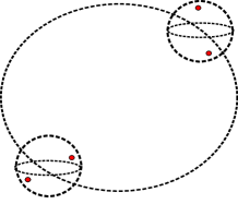
Figure 1. An illustration of $q_{1,2}\in H_{5}(B{\mathcal{S}}_{4})$.

We now present “linear” geometric representatives for cohomology classes.

Definition 4.6.

Let $\hat{X}$ be a manifold without boundary of dimension $nd-m$ which maps properly to $\overline{\rm Conf}_{n}({\mathbb{R}}^{d})$. We define its Thom class as follows. Take the fundamental class in mod-two locally-finite homology of $\hat{X}$ in dimension $nd-m$, and map it to locally-finite homology of $\overline{\rm Conf}_{n}({\mathbb{R}}^{d})$. Apply the Poincaré duality isomorphism to obtain a class in in $H^{m}(\overline{\rm Conf}_{n}({\mathbb{R}}^{d});{\mathbb{F}}_{2})$, which we call the Thom class of $\hat{X}$. By abuse we may sometimes refer only to the image of $\hat{X}$.

If we choose $d$ large enough (greater than $m$), then the restriction map from the cohomology of $\overline{\rm Conf}_{n}({\mathbb{R}}^{\infty})=B{\mathcal{S}}_{n}$ to that of $\overline{\rm Conf}_{n}({\mathbb{R}}^{d})$ is an isomorphism in degree $m$. (One can deduce this isomorphism from calculations in homology, which for $\overline{\rm Conf}_{n}({\mathbb{R}}^{d})$ is constructed from $q_{I}$ with $i_{k}<d$.) So this Thom class lifts uniquely to define a class in the cohomology of $B{\mathcal{S}}_{n}$ which we also call the Thom class.

For example, if we refer to points in $\overline{\rm Conf}_{n}({\mathbb{R}}^{d})$ as ${\bf x}=(x_{1},\ldots,x_{n})/\sim$, then the non-zero class in $H^{1}(\overline{\rm Conf}_{n}({\mathbb{R}}^{d}))$ for $d\geq 2$ is represented by the variety $X$ of points such that some $x_{i}$ and $x_{j}$ share their first coordinate. Specifically, let $\hat{X}$ be the space of configurations of $n$ points, two of which have one color - say black - and the rest of which share another color, such that the two black points must share their first coordinate. The Thom class of $\hat{X}$ mapping to the configuration space by forgetting colors is the non-trivial class in degree one, as we can see by evaluating it on the cycle $q_{1}$ by intersection (exactly once do two unlabeled points which are antipodal on some generic $S^{1}$ share their first coordinate).

Such Thom classes represent Hopf ring generators of the mod-two cohomology of symmetric groups.

Definition 4.7.

Let $q_{\ell\cdot 1}$ denote $q_{1,\ldots,1}$ and similarly let $q_{k\cdot 0,\ell\cdot 1}$ denote $q_{0,\ldots,0,1,\ldots,1}={q_{1,\ldots,1}}^{*2^{k}}$ in $H_{2^{k}(2^{\ell}-1)}(B{\mathcal{S}}_{2^{k+\ell}})$, where there are $k$ zeros and $\ell$ ones.

Let $\gamma_{\ell,n}$ denote the linear dual to ${(q_{\ell\cdot 1})}^{*n}$ in the Nakaoka monomial basis.

If $\alpha\in H^{*}(\coprod_{n}B{\mathcal{S}}_{n})$ is a monomial in the $q_{I}$ we let $\alpha^{\vee}\in H^{*}(\coprod_{n}B{\mathcal{S}}_{n})$ denote the cohomology class which evaluates to one on $\alpha$ and is zero on all other monomials. In particular $\gamma_{\ell,2^{k}}$ is ${q_{k\cdot 0,\ell\cdot 1}}^{\vee}$. We will use these $\gamma_{\ell,n}$ as Hopf ring generators for the cohomology of symmetric groups, thus making the following the first step in geometrically representing this cohomology.

Definition 4.8.

Let $\Gamma_{\ell,n}$ be defined as the collection of ${\bf x}=(x_{1},\cdots,x_{n2^{\ell}})/\sim$ which can be partitioned into $n$ sets of $2^{\ell}$ points such that all points in each set share their first coordinate.

$\Gamma_{\ell,n}$ is the image in $\overline{\rm Conf}_{n\cdot 2^{\ell}}({\mathbb{R}}^{d})$ of $\widehat{\Gamma_{\ell,n}},$ in which along with the points there is a choice of partition.

Theorem 4.9.

The cohomology class $\gamma_{\ell,n}$ is the Thom class of the variety $\Gamma_{\ell,n}$.

We first record the following, which is immediate algebraically from the definition.

Lemma 4.10.

The coproduct of $\gamma_{\ell,n}$ is given by

$$\Delta\gamma_{\ell,n}=\sum_{i+j=n}{\gamma_{\ell,i}}\otimes{\gamma_{\ell,j}}.$$

Proof of Theorem 4.9.

We start by showing that the coproduct formula of Lemma 4.10 holds for the the Thom class of $\Gamma_{\ell,n}$. We model the product map by the embedding $\overline{\rm Conf}_{i2^{\ell}}({\mathbb{R}}^{\infty})\times\overline{\rm Conf}_{(n-i)2^{\ell}}({\mathbb{R}}^{\infty})\to\overline{\rm Conf}_{n2^{\ell}}({\mathbb{R}}^{\infty})$ by using homeomorphism of ${\mathbb{R}}$ with the negative (respectively positive) real numbers to change the first coordinates of the first (respectively second) given configurations and taking their union. This model of the product map is transversal to $\Gamma_{\ell,n}$, whose preimage in $\overline{\rm Conf}_{i2^{\ell}}({\mathbb{R}}^{\infty})\times\overline{\rm Conf}_{(n-i)2^{\ell}}({\mathbb{R}}^{\infty})$ is exactly $\Gamma_{\ell,i}\times\Gamma_{\ell,n-i}.$ Because the Thom class of a preimage of a subvariety under a transversal map is the pull-back of its Thom class, the desired coproduct formula follows.

By Nakaoka’s calculation as stated in Theorem 4.3, the indecomposables in homology of $\bigsqcup_{n}B{\mathcal{S}}_{n}$ under the product lie in dimensions greater than $n-1$ on components indexed by $n$ which are powers of two. The product map is thus surjective in lower degrees, or dually the coproduct map is injective, which implies that we may use these coproduct formulae inductively to reduce to showing that the Thom class of $\Gamma_{\ell,1}$ is $\gamma_{\ell,1}$. Still using the coproduct formula, along with compatibility of evaluation of cohomology on homology with the product and coproduct, the value of $\Gamma_{\ell,1}$ on any product is zero. In degree $(2^{\ell}-1)$ the only indecomposible in homology is $q_{\ell\cdot 1}$. We can check immediately that ${\rm Orb}_{\ell\cdot 1}$ which represents $q_{\ell\cdot 1}$ intersects with $\Gamma_{\ell,1}$ in exactly one point, and the tangent vectors span the full tangent space of the configuration space as needed for transversality, as we illustrate in Figure 2. ∎

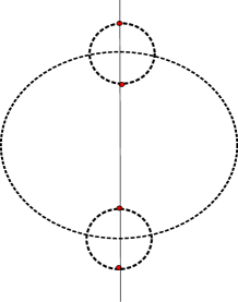
Figure 2. An illustration that $\Gamma_{2,1}$ intersects ${\rm Orb}_{1,1}$ exactly once.

These varieties $\Gamma_{\ell,n}$ are analogues of Schubert varieties, as we will see more precisely in Section 10. We can use other coordinates, or codimension one subspaces, to define $\Gamma_{\ell,n}$ and then use the geometry of cup and transfer products to understand representing varieties. For example, $\gamma_{1,2}\gamma_{2,1}$ is Thom class of the subvariety defined by “four points which share their first coordinate and break up into two groups of two points which share their second coordinate,” while $\gamma_{1,1}^{3}\odot\gamma_{1,1}$ is the Thom class of the subvariety defined by configurations with “two points which share their first three coordinates and another two which share their fourth coordinate.”

Getting back to homology, on the $q_{I}$ the coproduct dual to the cup product is classically known, and thus it is determined on the entire homology of symmetric groups because of the bialgebra structure.

Definition 4.11.

Define a coproduct $\Delta_{\cdot}$ on $H_{*}(\coprod_{n}B{\mathcal{S}}_{n})$ by extending the formula for $I$ admissible $\Delta_{\cdot}(q_{I})=\sum_{J+K=I}q_{J}\otimes q_{K}$ , where when $I=i_{1},\cdots,i_{n}$ we have that $J$ and $K$ range over partitions of the same length such that for each $\ell$, $j_{\ell}+k_{\ell}=i_{\ell}$.

This coproduct is more complicated than it seems at first. Even when starting with an admissible $I$, the sum above is over all possible $J$ and $K$. Thus to get an expression in the standard basis, as needed for example to apply the coproduct again, one must apply Adem and $q_{0}$ relations. The ones which get used most often are the relations $q_{2n+1}q_{0}=0$ and $q_{2n}q_{0}=q_{0}q_{n}$.

Theorem 4.12 (See for example I.2 of [9]).

Under the isomorphism of Theorem 4.3, the diagonal map on $\coprod_{n}B{\mathcal{S}}_{n}$ induces the map $\Delta_{\cdot}$ on homology.

On the other hand, one of our main results is that the coproduct dual to the transfer product is primitive. We originally proved this geometrically, but now by Kuhn’s suggestion we use the machinery of [8].

Theorem 4.13.

The transfer product is linearly dual to the primitive coproduct on the Kudo-Araki-Dyer-Lashof algebra. That is, $\Delta_{\odot}(q_{I})=q_{I}\otimes 1+1\otimes q_{I}$, where $1$ is the non-zero class in $H_{0}(B{\mathcal{S}}_{0})$.

Proof.

Let $D_{k}(Y)=E{\mathcal{S}}_{k}\ltimes_{{\mathcal{S}}_{k}}Y^{k}$, for a based space $Y$. We recall that $D(Y)=\bigvee_{k\geq 0}D_{k}(Y)$ is the free $E_{\infty}$-space $Y$, so in particular $D(S^{0})=\bigvee_{n\geq 0}B{\mathcal{S}}_{n}$. Similarly for a spectrum ${\mathcal{S}}$ we denote by ${\mathcal{D}}({\mathcal{S}})$ the free $E_{\infty}$-spectrum it generates. In particular ${\mathcal{D}}(\Sigma^{\infty}Y)\simeq\Sigma^{\infty}D(Y)$.

As mentioned in Remark 3.3, the transfer product is induced by a stable map

$$\Psi:\Sigma^{\infty}D(S^{0})\to\Sigma^{\infty}\left(D(S^{0})\wedge D(S^{0})\right).$$

Observe that there is an equivalence $\beta:D(S^{0}\vee S^{0})\simeq D(S^{0})\wedge D(S^{0})$.

Recall Theorem 4.3, which says that $H_{*}(D(S^{0}))$ is the free ${\mathcal{K}}$-algebra on the generator $\iota\in\tilde{H}_{0}(S^{0})$. Similarly, $H_{*}(D(S^{0}\vee S^{0}))$ is the free ${\mathcal{K}}$-algebra on the two generators

$$(\iota,0),(0,\iota)\in\tilde{H}_{0}(S^{0}\vee S^{0}).$$

Clearly $\beta_{*}(\iota,0)=\iota\otimes 1$ and $\beta_{*}(0,\iota)=1\otimes\iota$.

Theorem 1.5 in [8] states that $\Psi$ can be identified to $\mathcal{D}(v):{\mathcal{D}}(\underline{S}^{0})\to{\mathcal{D}}(\underline{S}^{0}\vee\underline{S}^{0})$, where $v:\underline{S}^{0}\to\underline{S}^{0}\vee\underline{S}^{0}$ is the pinch map of the sphere spectrum.

This implies that $\Delta_{\odot}$ is a map of ${\mathcal{K}}$-algebras. Explicitly, by the external Cartan formula,

$$\Delta_{\odot}q_{n}(a)=\sum_{i+j=n}(q_{i}\otimes q_{j})\Delta_{\odot}(a),$$

for $a\in H_{*}(\coprod_{n}B{\mathcal{S}}_{n})$. The class $\iota$ is clearly primitive since $v_{*}(\iota)=(\iota,0)+(0,\iota)$ implies $\Delta_{\odot}(\iota)=\iota\otimes 1+1\otimes\iota$. The external Cartan formula and the vanishing property of Definition 4.2 imply that $q_{I}$ is primitive for each $I$ by induction on the length of $I$, completing the proof.

∎

We use this theorem to quickly determine the cohomology of symmetric groups as a Hopf ring.

5. Hopf ring structure through generators and relations

The primitivity of the transfer coproduct coupled with some classical theorems immediately leads to algebraic presentations of $H^{*}(\coprod_{n}B{\mathcal{S}}_{n})$. Recall from Theorem 7.15 of Milnor and Moore’s standard reference [20] that a Hopf algebra which is polynomial and primitively generated has a linear dual that is exterior, generated by linear duals (in the monomial basis) to generators raised to powers of two. Theorem 4.13 implies the following.

Corollary 5.1.

Under the transfer product $\odot$ alone, the cohomology of $\coprod_{n}B{\mathcal{S}}_{n}$ is an exterior algebra, generated by $({q_{I}}^{*2^{k}})^{\vee}$ for $I$ strongly admissible, or equivalently by ${q_{I}}^{\vee}$ for $I$ admissible.

To incorporate the cup product structure, we appeal to another classical theorem. As in I.3 of [9], let $R[n]$ be the span of the $q_{I}$ of length $n$, a submodule of $H_{*}(B{\mathcal{S}}_{2^{n}})$. Recall that $\gamma_{\ell,m}$ is the linear dual to ${(q_{\ell\cdot 1})}^{*m}$ in the Nakaoka basis.

Theorem 5.2 (Theorem I.3.7 of [9]).

The linear dual of $R[n]$, which is an algebra under cup product, is isomorphic to the polynomial algebra generated by the classes $\gamma_{\ell,2^{k}}$ with $k+\ell=n$, which we denote $D_{n}$.

In Section 7 we review the classical fact that $D_{n}$ is canonically isomorphic to the $n$th Dickson algebra. For a sketch of proof of Theorem 5.2, it is simple to see that $q_{0,\ldots,0,1,\ldots,1}$ are primitive under $\Delta_{\cdot}$ because $q_{1}\circ q_{0}=0$. It is a straightforward induction to show there are no other primitives, and then a counting argument to show that there are no relations among the ${q_{k\cdot 0,\ell\cdot 1}}^{\vee}$. Note however that because of the Adem relations in the Kudo-Araki-Dyer-Lashof algebra, the pairing between $q_{I}$ and polynomials in $\gamma_{\ell,2^{k}}=(q_{\ell\cdot 0,k\cdot 1})^{\vee}$ is complicated. For example, ${\gamma_{1,2}}^{3}=({q_{0,1}}^{\vee})^{3}={q_{0,3}}^{\vee}+{q_{2,2}}^{\vee},$ in part since $\Delta_{\cdot}q_{2,2}$ includes as a term $q_{2,0}\otimes q_{0,2}$, which is equal to $q_{0,1}\otimes q_{0,2}$.

Theorem 5.2 gives us the last input we need to understand the cohomology of symmetric groups as a Hopf ring, since we see that under $\odot$ alone the generators are polynomials in the $\gamma_{\ell,2^{k}}$.

Theorem 5.3.

As a Hopf ring, $H^{*}(\coprod_{n}B{\mathcal{S}}_{n})$ is generated by the classes $\gamma_{\ell,2^{k}}$.

The transfer product is exterior, and the antipode map is the identity. The $\gamma_{\ell,2^{k}}$ with $\ell+k=n$ form a polynomial ring.

The stated facts along with Hopf ring distributivity and the fact that the products of classes on different components are zero determine the cup product structure, in particular of individual components.

Corollary 5.4.

Any collection of classes $\{\alpha_{\ell,2^{k}}\}$ such that $\alpha_{\ell,2^{k}}\in H^{2^{k}(2^{\ell}-1)}(B{\mathcal{S}}_{2^{k+\ell}})$ pairs non-trivially with $q_{k\cdot 0,\ell\cdot 1}$ constitutes a generating set for $H^{*}(\coprod_{n}B{\mathcal{S}}_{n})$ as a Hopf ring.

In order to apply the distributivity relation, we need the coproduct of $\gamma_{\ell,2^{k}}$ as given by Lemma 4.10. Finally, we compute transfer products by taking the binary expansion $j=\sum 2^{k_{i}}$ with $k_{i}$ distinct, so that ${q_{\ell\cdot 1}}^{*j}=\prod{q_{\ell\cdot 1}}^{*2^{k_{i}}}$. By Theorem 4.13 and linear duality it follows that

$$\gamma_{\ell,j}=\bigodot_{j=\sum 2^{k_{i}}}\gamma_{\ell,2^{k_{i}}}.$$

Because the transfer product is exterior, we obtain the following.

Proposition 5.5.

The transfer products of classes $\gamma_{\ell,n}$ are given by

$$\gamma_{\ell,n}\odot\gamma_{\ell,m}=\binom{n+m}{n}\gamma_{\ell,n+m},$$

while transfer products between other classes have no relations.

Collecting Theorem 5.3, Lemma 4.10, Theorem 5.2 and Proposition 5.5 yields a proof of Theorem 1.2, our first presentation of the cohomology of symmetric groups as a Hopf ring.

Theorem 5.3 and the fact that transfer product is exterior leads to an additive basis for the cohomology of symmetric groups. Since the $\gamma_{\ell,2^{k}}$ are Hopf ring generators, their Hopf ring monomials span, and an induction by number of transfer products using Theorem 4.13 shows they are independent. Let ${\mathcal{P}}(m)$ denote the set of partitions of $m$ into nonnegative powers of two. If $P$ is such a partition, let $P_{n}$ denote the number of times $2^{n}$ occurs, and let $D_{P}$ denote $\bigotimes_{n}\bigwedge^{P_{n}}D_{n}$ where $D_{n}$ is the polynomial algebra on $\gamma_{\ell,2^{k}}$ with $\ell+k=n$ as stated in Theorem 5.2. By convention $D_{0}$ is the ground field. We recover an additive isomorphism well-known to experts.

Proposition 5.6.

As a graded vector space, $H^{*}(BS_{n})$ is isomorphic to $\bigoplus_{P\in{\mathcal{P}}(n)}D_{P}$.

It is straightforward to calculate the Poincaré polynomial for this cohomology. We have found it unenlightening since we could only describe Poincaré polynomials of exterior powers of polynomial algebras using inclusion-exclusion methods.

In the next section we develop a slightly improved basis, which requires the following.

Proposition 5.7.

The classes $\{\gamma_{\ell,n}\}$ such that $n2^{\ell}=m$ generate a polynomial subalgebra of $H^{*}(B{\mathcal{S}}_{m})$.

Sketch of proof..

We start with $m=2^{p}$ which is covered by Theorem 5.2, which says that the classes $\gamma_{\ell,2^{k}}$ with $k+\ell=p$ form a polynomial subring of $H^{*}(B{\mathcal{S}}_{2^{p}})$. We then use in induction on the number of ones in the binomial expansion of $m$ and Hopf ring distributivity to establish the general case. ∎

15								$\gamma_{4,1}$
14								$\gamma_{3,2}$
13
12								$\gamma_{2,4}$
11
10
9						$\gamma_{2,3}$
8								$\gamma_{1,8}$
7				$\gamma_{3,1}$			$\gamma_{1,7}$
6				$\gamma_{2,2}$		$\gamma_{1,6}$
5					$\gamma_{1,5}$
4				$\gamma_{1,4}$
3		$\gamma_{2,1}$	$\gamma_{1,3}$
2		$\gamma_{1,2}$
1	$\gamma_{1,1}$
	$B{\mathcal{S}}_{2}$	$B{\mathcal{S}}_{4}$	$B{\mathcal{S}}_{6}$	$B{\mathcal{S}}_{8}$	$B{\mathcal{S}}_{10}$	$B{\mathcal{S}}_{12}$	$B{\mathcal{S}}_{14}$	$B{\mathcal{S}}_{16}$

Figure 3. Hopf ring generators of $H^{*}(\coprod_{n}B{\mathcal{S}}_{n})$ through $B{\mathcal{S}}_{16}$.

By Theorem 5.3 that $\gamma_{\ell,n}$ are Hopf ring generators, Theorem 4.9 that these classes are Thom classes of linear subvarieties, and the geometric interpretations of cup and transfer products, all of the cohomology of symmetric groups is represented by such subvarieties. These are defined by groupings and subgroupings of points into sets with cardinalities which are powers of two which share coordinates. The third author began this investigation by conjecturing that representations by linear subvarieties would be possible, since linear submanifolds represent classes in ordered configuration spaces.

6. Presentation of product structures through an additive basis

We can use our knowledge of the Hopf ring structure on $H^{*}(\coprod_{n}B{\mathcal{S}}_{n})$ to explicitly understand the cup and transfer product structures through additive bases. We set the notational conventions that cup product has priority over transfer product, so that $a\cdot b\odot c$ means $(a\cdot b)\odot c$, and that exponents always refer to repeated application of cup product (an easy choice, since transfer product is exterior). Let $1_{m}$ denote the unit for cup product on component $m$.

We proceed with some calculations on the first even components (since the ${\mathbb{F}}_{2}$-cohomology of $B{\mathcal{S}}_{2k+1}$ is isomorphic to that of $B{\mathcal{S}}_{2k}$.) As $B{\mathcal{S}}_{2}\simeq{\mathbb{R}}P^{\infty}$ its cohomology is a polynomial ring generated by $\gamma_{1,1}$.

For $H^{*}(B{\mathcal{S}}_{4})$ the Hopf ring monomial basis consists of classes ${\gamma_{1,1}}^{i}\odot{\gamma_{1,1}}^{j}\in H^{i+j}(B{\mathcal{S}}_{4})$ (which are zero if $i=j$) along with polynomials in $\gamma_{1,2}\in H^{2}(B{\mathcal{S}}_{4})$ and $\gamma_{2,1}\in H^{3}(B{\mathcal{S}}_{4})$. Using Hopf ring distributivity, we have that

$$({\gamma_{1,1}}^{i}\odot{\gamma_{1,1}}^{j})\cdot({\gamma_{1,1}}^{k}\odot{\gamma_{1,1}}^{\ell})={\gamma_{1,1}}^{i+k}\odot{\gamma_{1,1}}^{j+\ell}+{\gamma_{1,1}}^{i+\ell}\odot{\gamma_{1,1}}^{j+k},$$

where we note one of these terms could be zero, if either $i+k=j+\ell$ or if $i+\ell=j+k$. In order to compute some products with $\gamma_{1,2}$ we have to use its coproduct, which by Lemma 4.10 is equal to $\gamma_{1,2}\otimes 1_{0}+\gamma_{1,1}\otimes\gamma_{1,1}+1_{0}\otimes\gamma_{1,2}$. Using distributivity,

$$\gamma_{1,2}\cdot({\gamma_{1,1}}^{n}\odot{\gamma_{1,1}}^{m})=(\gamma_{1,2}\cdot{\gamma_{1,1}}^{n})\odot(1_{0}\cdot{\gamma_{1,1}}^{m})+\\ (\gamma_{1,1}\cdot{\gamma_{1,1}}^{n})\odot(\gamma_{1,1}\cdot{\gamma_{1,1}}^{m})+(1_{0}\cdot{\gamma_{1,1}}^{n})\odot(\gamma_{1,2}\cdot{\gamma_{1,1}}^{m})={\gamma_{1,1}}^{n+1}\odot{\gamma_{1,1}}^{m+1}.$$$$

In general, most terms arising from the Hopf ring distributivity relation are zero because they involve multiplication of classes supported on different components. The last basic products to compute for $B{\mathcal{S}}_{4}$ are $\gamma_{2,1}\cdot({\gamma_{1,1}}^{n}\odot{\gamma_{1,1}}^{m})$, which are zero because the coproduct of $\gamma_{2,1}$ is just $\gamma_{2,1}\otimes 1_{0}+1_{0}\otimes\gamma_{2,1}.$ Applying distributivity repeatedly we get that if $k\neq 0$

$${\gamma_{1,2}}^{p}{\gamma_{2,1}}^{q}\cdot({\gamma_{1,1}}^{k}\odot{\gamma_{1,1}}^{\ell})=\begin{cases}{\gamma_{1,1}}^{k+p}\odot{\gamma_{1,1}}^{\ell+p}\;\;\;&{\rm if}\;\;q=0.\\ 0\;\;\;\;\;\;&{\rm if}\;\;q\neq 0,\end{cases}$$

which completes an understanding of how to multiply elements of our additive basis. The case of $B{\mathcal{S}}_{4}$ is one of the very few in which it is simpler to understand the cup multiplicative structure in terms of ring generators and relations. From the multiplicative rules just given, it is a straightforward exercise to deduce that $\gamma_{1,1}\odot 1_{2}$, $\gamma_{1,2}$ and $\gamma_{2,1}$ generate the cohomology on this component, with the lone relation being $(\gamma_{1,1}\odot 1_{2})\cdot\gamma_{2,1}=0$. Similarly, one can write down an additive basis for $H^{*}(B{\mathcal{S}}_{6})$, determine its multiplication rules, and then show that it is generated by $\gamma_{1,1}\odot 1_{4}$, $\gamma_{1,2}\odot 1_{2}$, $\gamma_{2,1}\odot 1_{2}$ and $\gamma_{1,1}^{2}\odot\gamma_{1,1}\odot 1_{2}$, with the relation that $\gamma_{2,1}\cdot({\gamma_{1,1}}^{2}\odot\gamma_{1,1}\odot 1_{2})=0$, in agreement with the results of Chapter VI.5 of [3].

Remark 6.1.

We can also see relations through our geometric representatives for cohomology. For example, $\gamma_{2,1}\cdot(\gamma_{1,1}\odot 1_{2})$ is represented by the subvariety of “four points which share their first coordinate, two of which share their second coordinate.” This subvariety is cobounded by “four points, two of which share their first coordinate, two of which share their first and second coordinate, with the first two having a first coordinate which is less than that of the second two.”

In general, presentations in terms of generators and relations are quite complicated. We instead understand cup and transfer products explicitly in terms of a canonical additive basis. Recall the notion of Hopf ring monomial from Definition 2.5.

Definition 6.2.

A gathered monomial in the cohomology of symmetric groups is a Hopf ring monomial in the generators $\gamma_{\ell,n}$ where such $n$ are maximal or equivalently the number of transfer products which appear is minimal.

For example, $\gamma_{1,4}{\gamma_{2,2}}^{3}\odot\gamma_{1,2}{\gamma_{2,1}}^{3}=\gamma_{1,6}{\gamma_{2,3}}^{3}$. Gathered monomials such as the latter in which no transfer products appear are building blocks for general gathered monomials.

Definition 6.3.

A gathered block is a monomial of the form $\prod_{i}{\gamma_{\ell_{i},n_{i}}}^{d_{i}},$ where the product is the cup product. Its profile is defined to be the collection of pairs $(\ell_{i},d_{i})$.

Non-trivial gathered blocks must have all of the numbers $2^{\ell_{i}}n_{i}$ equal, and we call this number divided by two the width. We assume that the factors are ordered from smallest to largest $n_{i}$ (or largest to smallest $\ell_{i}$), and then note that $n_{i}=2^{\ell_{1}-\ell_{i}}n_{1}$.

Proposition 6.4.

A gathered monomial can be written uniquely as the transfer product of gathered blocks with distinct profiles. Gathered monomials form a canonical additive basis for the cohomology of $\coprod_{n}B{\mathcal{S}}_{n}$.

Representing gathered monomials graphically is helpful. We represent $\gamma_{\ell,n}$ by a rectangle of width $n\cdot 2^{\ell}$ and height $1-\frac{1}{2^{\ell}}$, so that its area corresponds to its degree. We represent $1_{n}$ by an edge of width $n$ (a height-zero rectangle). A gathered block, which is a product of $\gamma_{\ell,n}$ for fixed $n\cdot 2^{\ell}$, is represented by a single column of such rectangles, stacked on top of each other, with order which does not matter. A gathered monomial is represented by placing such columns next to each other, which we call the skyline diagram of the monomial. We also refer to the gathered monomial basis as the skyline basis to emphasize this presentation. See Figure 4 below for an illustration.

Definition 6.5.

Let $\prod_{i}{\gamma_{\ell_{i},n_{i}}}^{d_{i}}$ be a gathered block, and let $n_{1}=\sum_{j=1}^{k}m_{j}$ be a partition of $n_{1}$. A partition of this gathered block into $k$ is defined by the set consisting of the $k$ blocks $\prod_{i}{\gamma_{\ell_{i},2^{\ell_{1}-\ell_{i}}m_{j}}}^{d_{i}}.$ We allow for some $m_{j}$ to be zero, in which case the corresponding elements of the partition will be $1_{0}$.

A splitting of a gathered monomial $f_{1}\odot\cdots\odot f_{k}$ into two is a pair of gathered monomials $f_{1}^{\prime}\odot\cdots\odot f_{k}^{\prime}$ and $f_{1}^{\prime\prime}\odot\cdots\odot f_{k}^{\prime\prime}$ where each $\{f_{i}^{\prime},f_{i}^{\prime\prime}\}$ is a partition of $f_{i}$ into two (which could be trivial - that is, of the form $\{1_{0},f_{i}\}$).

Proposition 6.6.

The coproduct of a gathered monomial is given by

$$\Delta f_{1}\odot\cdots\odot f_{k}=\left(\sum f_{1}^{\prime}\odot\cdots\odot f_{k}^{\prime}\right)\otimes\left(f_{1}^{\prime\prime}\odot\cdots\odot f_{k}^{\prime\prime}\right),$$

where the sum is over all splittings of the monomial into two.

Proof.

To establish the special case of gathered blocks - that is, having only one $f$ - we use the Hopf algebra compatibility of cup product and Pontryagin coproduct. The coproduct $\Delta$ of any ${\gamma_{\ell_{i},n_{i}}}^{d_{i}}$ will correspond to partitions of $n_{i}$ into two. But only for the partitions of $n_{1}$ will there be corresponding partitions for all $n_{i}$ which yield non-trivial classes when cupped together. The resulting products correspond to the partitions of $f$ into two.

The general case follows from the Hopf algebra compatibility of partition product and Pontryagin coproduct. Because the monomial is gathered, no terms in the coproducts of $f_{i}$ can be equal, so we obtain no trivial transfer products when such terms are collected. ∎

In terms of skyline diagrams, the coproduct can be understood by introducing vertical dashed lines in the rectangles representing $\gamma_{\ell,n}$, dividing the rectangle into $n$ equal pieces. The coproduct is then given by dividing along all existing columns and vertical dashed lines of full height and then partitioning them into two to make two new skyline diagrams.

Definition 6.7.

A partition of a gathered monomial in $H^{*}(B{\mathcal{S}}_{m})$ is a partition of each of its gathered blocks. The associated component partition is the partition of $m$ given by the components of the classes in the partition.

We define the refinement of a partition of a gathered monomial in the obvious way, reflected faithfully by the refinement structure of the associated component partitions.

A matching $\mu$ between partitions of two gathered monomials is an isomorphism of their respective component partitions. We say that one matching refines another if that isomorphism commutes with inclusions of components under refinement.

For any gathered monomial in $H^{*}(B{\mathcal{S}}_{m})$ there is a canonical partition of $m$ defined by the components of its constituent gathered block monomials. The associated component partition of a monomial partition is a refinement of this canonical partition.

We are now ready to describe product structures in terms of our additive basis of gathered monomials.

Theorem 6.8.

The transfer product of two gathered monomials ${\bf m}$ and ${\bf n}$ is a multiple of the gathered monomial whose gathered block of a given profile has width which is the sum of the widths of the blocks of that profile in ${\bf m}$ and ${\bf n}$. The multiple is zero if and only if any of those two widths share some non-zero digit of their binary expansion.

Let $M_{{\bf m},{\bf n}}$ denote the set of matchings between any of the partitions of these gathered monomials which are not a refinement of some other matching. The cup product of $x$ and $y$ is the sum

$$\sum_{\mu\in M_{{\bf m},{\bf n}}}\left(\bigodot_{b,b^{\prime}{\textrm{ matched by }}\mu}\beta_{\mu}b\cdot b^{\prime}\right),$$

where $\beta_{\mu}$ is zero if and only if there are two products $b\cdot b^{\prime}$ which result in blocks with the same profile and whose widths have binary expansion which share a non-zero digit.

Graphically, transfer product corresponds to placing two column Skyline diagrams next to each other and merging columns with the same constituent blocks, with a coefficient of zero if any of those column widths share a one in their dyadic expansion. For cup product, we start with two column diagrams and consider all possible ways to split each into columns, along either original boundaries of columns or along the vertical lines of full height internal to the rectangles representing $\gamma_{\ell,n}$. We then match columns of each in all possible ways up to automorphism, and stack the resulting matched columns to get a new set of columns – see the Figure 4.

$\cdot$

=

+

(a) $(\gamma_{1,1}^{i}\odot\gamma_{1,1}^{j})\cdot(\gamma_{1,1}\odot 1_{2})=\gamma_{1,1}^{i+1}\odot\gamma_{1,1}^{j}+\gamma_{1,1}^{i}\odot\gamma_{1,1}^{j+1}$

$\cdot$

=

(b) $(\gamma_{1,1}^{i}\odot\gamma_{1,1}^{j})\cdot\gamma_{1,2}=\gamma_{1,1}^{i+1}\odot\gamma_{1,1}^{j+1}$

$\cdot$

=

0

(c) $(\gamma_{1,1}^{i}\odot\gamma_{1,1}^{j})\cdot\gamma_{2,1}=0$

$\cdot$

=

+

(d) $(\gamma_{1,1}^{3}\odot\gamma_{2,1}\odot 1_{2})\cdot(\gamma_{1,2}\odot 1_{4})=\gamma_{1,1}^{4}\odot\gamma_{2,1}\odot 1_{2}+\gamma_{1,1}^{3}\odot\gamma_{1,2}\gamma_{2,1}\odot 1_{2}$

Figure 4. Some computations in $H^{*}(B{\mathcal{S}}_{4})$ and $H^{*}(B{\mathcal{S}}_{8})$, expressed by both gathered monomials and skyline diagrams.

Proof of Theorem 6.8.

We use gathered blocks, whose multiplication is polynomial by Proposition 5.7 as a base case for an induction on the total number of blocks in ${\bf m}$ and ${\bf n}$. View say ${\bf m}$ as a non-trivial transfer product of ${\bf m}^{\prime}$ and ${\bf m}^{\prime\prime}$ which preserves blocks, so that ${\bf m}^{\prime}$ and ${\bf m}^{\prime\prime}$ each has fewer blocks than ${\bf m}$. The key is to see that each matching in $M_{{\bf m},{\bf n}}$ coincides with some (arbitrary) partition of $y$ into $\{{\bf n}^{\prime},{\bf n}^{\prime\prime}\}$ along with matchings of partitions of those pieces with partitions of ${\bf m}^{\prime}$ and ${\bf m}^{\prime\prime}$. From this observation, the induction follows, with the coefficient $\beta_{\mu}$ accounting for when such a process yields a partition product of some monomial in the $\gamma_{\ell,2^{k}}$ with itself. ∎

Given that the basis of skyline diagrams is a fundamental cohomology basis, it would be helpful to understand the pairing of gathered monomials with Nakaoka’s monomial basis for homology. Polynomials in $\gamma_{\ell,2^{k}}$ are the fundamental case, which as mentioned after Theorem 5.2 pair non-trivially with the basis of $q_{I}$ with $I$ of length $k+\ell$.

7. Topology and the invariant theoretic presentation

Compare the presentation for the cohomology of symmetric groups as a Hopf ring, as given in Theorem 1.2, with the Hopf ring presentations of rings of symmetric functions, as given in Example 2.6 and Proposition 2.8. Seeing classes which behave similarly, we obtain some immediate identifications of split quotient rings of the cohomology of symmetric groups.

Definition 7.1.

Define the level-$\ell$ quotient Hopf ring of the cohomology of symmetric groups, denoted ${\mathcal{P}}_{\ell}$, to be the quotient Hopf ring obtained by setting all $\gamma_{\ell^{\prime},n}$ for $\ell^{\prime}\neq\ell$ equal to zero. This quotient map is split by the sub-Hopf ring generated by the classes $\gamma_{\ell,n}$. Let ${\mathcal{P}}_{\ell}[m]$ be the sub-module of ${\mathcal{P}}_{\ell}$ supported on $B{\mathcal{S}}_{m}$, which is an algebra under cup product.

Graphically, these sub-rings each consist of all skyline diagrams made from the blocks of one fixed size.

Proposition 7.2.

The level-$\ell$ Hopf ring ${\mathcal{P}}_{\ell}$ is isomorphic as Hopf ring to the total symmetric invariants of a ${\bf k}[x]$. Thus ${\mathcal{P}}_{\ell}[m]$ is a polynomial ring for any $m$.

The proof is an immediate comparison of their two presentations. We originally proved the second part directly from the Hopf ring presentation of ${\mathcal{P}}_{\ell}[m]$, before realizing that we were mimicking the proof that symmetric functions form a polynomial algebra.

This identification has the following significant generalization.

Definition 7.3.

Define the scale of $\gamma_{\ell,n}$ to be the product $\ell\cdot|n|_{2}$, where $|n|_{2}$ is the $2$-adic valuation of $n$ (that is, the largest power of two which divides $n$). Define the scale-$k$ quotient of the cohomology of symmetric groups, denoted ${\mathcal{Q}}_{k}$, to be the quotient Hopf ring obtained by setting all $\gamma_{\ell,n}$ with either scale less than $k$ or with $\ell>k$ to zero. It is isomorphic to the sub-Hopf ring generated by $\gamma_{\ell,n}$ with scale greater than or equal to $k$ and $\ell\leq k$.

Graphically, the skyline diagrams which are non-zero in this quotient are those made up of blocks of width exactly $2^{k-1}$.

In the level-$\ell$ case, the split sub-ring was compatible with our additive basis, in that if a sum of gathered monomials was in the sub-ring then each monomial was in the sub-ring itself. That is not true in the scale-$\ell$ setting, where for example ${\gamma_{1,2}}^{3}$ includes a term of ${\gamma_{1,1}}^{3}\odot{\gamma_{1,1}}^{2}\odot\gamma_{1,1}$.

Proposition 7.4.

The scale-$k$ Hopf ring ${\mathcal{Q}}_{k}$ is isomorphic as a Hopf ring to the total symmetric invariants of a polynomial ring in $k$ variables.

Once again, the proof is by a direct comparison, made possible by the Hopf ring approach. The canonical isomorphism between them sends $\gamma_{\ell,n}$ with scale greater than or equal to $k$ and $\ell\leq k$ to the symmetric polynomial $\sigma(\ell)_{m}$ with $m={\frac{n}{2^{k-\ell}}}$.

Our goals in the rest of this section are twofold. First we develop the standard topology which underlies these isomorphisms. Then, we move from these identifications of local invariant-theoertic sub/quotient rings to the global invariant-theoretic description of Theorem 7.10.

The predominant approach to the cohomology of symmetric groups has been through restricting cohomology to that of elementary abelian subgroups. For the following, we refer to Chapters 3 and 4 in [3]. Let $V_{n}$ denote the subgroup of $(\mathbb{Z}/2)^{n}\subset{{\mathcal{S}}}_{2^{n}}$ defined by having $(\mathbb{Z}/2)^{n}$ act on itself. If we view this action as given by linear translations on the ${\mathbb{F}}_{2}$-vector space $\oplus_{n}{{\mathbb{F}}_{2}}$, then we can see that the normalizer of this subgroup is isomorphic to all affine transformations of $({\mathbb{F}}_{2})^{n}$. The Weyl group is thus $GL_{n}({\mathbb{F}}_{2})$, which acts as expected on the cohomology of $V_{n}$. The invariants ${\mathbb{F}}_{2}[x_{1},\ldots,x_{n}]^{GL_{n}({\mathbb{F}}_{2})}$ are known as Dickson algebras, which are polynomial on generators $d_{k,\ell}$ in dimensions $2^{k}(2^{\ell}-1)$ where $k+\ell=n$. As mentioned earlier, these Dickson algebras together form a Hopf ring, which we are currently investigating.

Since we base our work on Nakaoka’s homology calculation, our analysis of elementary abelian subgroups involves homology as well as cohomology.

Lemma 7.5.

The image of the homology of $BV_{n}$ in that of $B{\mathcal{S}}_{2^{n}}$ is exactly the span of the $q_{I}$ for $I$ admissible of length $n$.

Proof.

The inclusion of $V_{n}$ into ${\mathcal{S}}_{2^{n}}$ factors through the $n$-fold iterated wreath product of $\mathbb{Z}/2$ with itself, that is $\mathbb{Z}/2\int\left(\mathbb{Z}/2\int\left(\cdots\left(\mathbb{Z}/2\int\mathbb{Z}/2\right)\cdots\right)\right)$. A well-known alternate definition of the Dyer-Lashof operations $q_{i}$ is through the homology of the inclusion of wreath products $\mathbb{Z}/2\int{\mathcal{S}}_{n}\to{\mathcal{S}}_{2n}$. Inductively, the image of this iterated wreath product is given by length-$n$ Kudo-Araki-Dyer-Lashof classes, so the image of $V_{n}$ is contained in the span of such operations.

To see that the image of $V_{n}$ yields all such classes we compare ranks using the dual map in cohomology. We claim that the image in cohomology of the inclusion of $V_{n}$ in ${\mathcal{S}}_{2^{n}}$ is all of the Dickson invariants ${\mathbb{F}}_{2}[x_{1},\ldots,x_{n}]^{GL_{n}({\mathbb{F}}_{2})}\cong{\mathbb{F}}_{2}[d_{k,\ell}]$ with $k+\ell=n$ and $\ell>0,$ a fact known by Milgram [18] which we share now. The standard representation of ${\mathcal{S}}_{2^{n}}$ through permutation matrices gives rise to a vector bundle. Because $V_{n}$ embeds in ${\mathcal{S}}_{2^{n}}$ through the linear action of $({\mathbb{F}}_{2})^{n}$ on itself, on passing to a permutation representation the standard representation yields the sum of all one-dimensional real representations of $(\mathbb{Z}/2)^{n}$. Thus when the corresponding bundle is pulled back to $BV_{n}$ it splits as the sum of all possible line bundles. So the total Stiefel-Whitney class of this standard bundle in the cohomology of $B{\mathcal{S}}_{2^{n}}$ maps to $\prod_{y\in H^{1}(BV_{n})}(1+y)$, where $y$ ranges over linear combinations of the $x_{i}$. But classical invariant theory identifies $\sum d_{k,\ell}$ with the product of all $1+\lambda$ where $\lambda$ varies over all linear functions in the $x_{i}$. So these Stiefel-Whitney classes map exactly to the Dickson generators (or to zero).

By Madsen’s calculation, Theorem I.3.7 of [9] as recounted in Theorem 5.2, the linear dual to the span of the length-$n$ $q_{I}$ is a polynomial algebra in classes of dimension $2^{k}(2^{\ell}-1)$ with $k+\ell=n$ and $\ell>0$. Since the image of the cohomology of $B{\mathcal{S}}_{2^{n}}$ in that of $BV_{n}$ has the same rank as this polynomial algebra, and thus as the span of $q_{I}$ of length $n$, the image in homology must be all of this span. ∎

Because the only classes in the Weyl-invariant cohomology of $BV_{n}$ in degrees $2^{k}(2^{\ell}-1)$ are the Dickson classes, and the map in homology sends a generator in that degree to $q_{k\cdot 0,\ell\cdot 1}$, we have the following.

Corollary 7.6.

The restriction of $\gamma_{\ell,2^{k}}$ with $k+\ell=n$ to the elementary abelian subgroup $V_{n}$ is the Dickson class $d_{k,\ell}$.

Following Quillen [23, 24], Gunawardena-Lannes-Zarati [11] showed that $H^{*}(B{{\mathcal{S}}}_{n})$ injects in the direct sum of the cohomology of elementary abelian subgroups. Lemma 7.5 gives an alternate proof for that theorem through the following refinement.

Corollary 7.7.

The image of the elementary abelian subgroup $\prod_{i}V_{k_{j}}$ in the homology of any symmetric group which contains it (that is, of order $\sum 2^{k_{j}}$ or greater) is the span of products $\prod q_{I_{j}}$ where $I_{j}$ is of length $k_{j}$. Thus, the map from the homology of all elementary abelian subgroups to the homology of symmetric groups is surjective.

We now give a topological interpretation of Proposition 7.4.

Theorem 7.8.

The map from $H^{*}(\coprod_{n}B{\mathcal{S}}_{n})$ to its image in the cohomology of $\coprod_{m}{BV_{k}}^{\frac{m}{2^{k}}}$ coincides with the quotient map defining the scale-$k$ quotient ring ${\mathcal{Q}}_{k}$.

Proof.

By Corollary 7.7, the image in homology of $\coprod_{m}{BV_{k}}^{\frac{m}{2^{k}}}$ is the submodule of products of $q_{I}$ of length $k$. By Theorem 4.12 and Theorem 4.13, it is closed under the coproducts dual to cup and transfer product. Thus the image of this map of classifying spaces in cohomology, linear dual to this image of homology, is a quotient of the cohomology of symmetric groups as a Hopf ring.

Recall that $\gamma_{\ell,n}=({q_{\ell\cdot 1}}^{*n})^{\vee}$, so that all $\gamma_{\ell,n}$ with either scale less than $k$ or $\ell>k$ will evaluate to zero on the image of homology. An elementary counting argument shows that this ideal, the quotient by which defines ${\mathcal{Q}}_{k}$, is as large as possible so that the restriction of the cohomology of symmetric groups to these elementary abelian subgroups is exactly ${\mathcal{Q}}_{k}$. ∎

We now give a global invariant theoretic description of the cohomology of symmetric groups.

Definition 7.9.

Consider the ring of polynomials ${\mathbb{F}}_{2}[x_{A}]$, where $A\subseteq\underline{m}=\{1,\ldots,m\}$. We call ${A^{\prime}}$ a translate of ${A}$ if they are disjoint and of the same cardinality. A collection of translates is to be mutually disjoint. Call a monomial $\prod x_{A_{i}}$ proper if whenever some $A_{i}$ and $A_{j}$ intersect, one is contained in the other, say $A_{i}\subset A_{j}$, and $A_{j}$ is the union of translates of $A_{i}$

Theorem 7.10.

The cohomology of symmetric groups $H^{*}(\coprod_{n}B{\mathcal{S}}_{n};{\mathbb{F}}_{2})$ is isomorphic to to the quotient of $\bigoplus_{m}{\mathbb{F}}_{2}[x_{A}|A\subset\underline{m}]^{{\mathcal{S}}_{m}}$, with $x_{A}$ in degree $2^{\#A}-1$, by the additive submodule consisting of symmetrizations of monomials which are not proper.

Sketch of proof..

We begin with the abstract Hopf ring description of $H^{*}(\coprod_{n}B{\mathcal{S}}_{n};{\mathbb{F}}_{2})$ given in Theorem 1.2, and show that it is isomorphic to the quotient stated.

Given some $A=\{1,\cdots,2^{k}\}\subset\underline{m}$ define its $i$th translate $\tau_{i}A$ to be $\{1+i2^{k},\cdots,(i+1)2^{k}\}$. We start to define a map between $H^{*}(\coprod_{n}B{\mathcal{S}}_{n};{\mathbb{F}}_{2})$ and this ring of invariants by sending $\gamma_{\ell,n}$ to $\prod_{i=1}^{n}x_{\tau_{i}A}$ where $A=\{1,\cdots,2^{\ell}\}$. More generally, the gathered block $\prod{\gamma_{\ell_{i},n_{i}}}^{d_{i}}$ maps to the symmetrized product where the first $n_{i}$ translates of $x_{1,\cdots,2^{\ell_{i}}}$ are raised to the $d_{i}$th power. Such products are proper monomials. The transfer products of gathered blocks go to symmetrized products of such monomials, after reindexing so that the subscripts corresponding to different gathered blocks are distinct. Just as we showed for symmetric functions in Proposition 2.8, with patience we can see that all proper symmetric monomials can, after reindexing, be put in this form. ∎

8. Steenrod algebra action

We now give a presentation of the cohomology of symmetric groups as algebras over the mod-two Steenrod algebra $\mathcal{A}$.

Proposition 8.1.

The Steenrod squares ${Sq^{i}}$ satisfy a Cartan formula with respect to transfer product. That is ${Sq^{i}}(\alpha\odot\beta)=\sum_{j+k=i}{Sq}^{j}\alpha\odot{Sq}^{k}\beta$.

Because transfers are stable maps, they preserve Steenrod squares. So this proposition is immediate from Definition 3.1 and the external Cartan formula. Because there are Cartan formulae with respect to both products, the cohomology of $\coprod_{n}B{\mathcal{S}}_{n}$ is a Hopf ring over the Steenrod algebra.

The Steenrod algebra structure on all of the cohomology of $\coprod_{n}B{\mathcal{S}}_{n}$ is thus determined by the action on Hopf ring generators, and we consider the minimal set of $\gamma_{\ell,2^{k}}$. We introduce some notation to describe the action of Steenrod squares on these classes, using the additive basis of gathered monomials for skyline diagrams from Section 6.

Definition 8.2.

• The height of a gathered monomial is the largest of the algebraic degrees of its gathered blocks. (The algebraic degree is the total number of Hopf ring generators cup-multiplied to give the gathered block.)

• The effective scale of a gathered block, which is a product of $\gamma_{\ell,n}$’s, is the largest $\ell$ which occurs. The effective scale of a gathered monomial is the minimum of the effective scales of its constituent blocks.

• We say a monomial is not full width if it is a non-trivial transfer product of some monomial with some $1_{k}$.

Theorem 8.3.

${Sq}^{i}\gamma_{\ell,2^{k}}$ is the sum of all full-width monomials of total degree $2^{k}(2^{\ell}-1)+i$, height one or two, and effective scale at least $\ell$.

We call such monomials the outgrowth monomials of $\gamma_{\ell,2^{k}}.$

For example,

$${Sq}^{3}\gamma_{2,4}=\gamma_{4,1}+\gamma_{3,1}\odot\gamma_{2,1}\gamma_{1,2}\odot\gamma_{2,1}+{\gamma_{2,1}}^{2}\odot\gamma_{2,1}\odot\gamma_{2,2}.$$

We can translate the conditions of Theorem 8.3 to our skyline diagrams, seeing that a Steenrod square on $\gamma_{\ell,2^{k}}$ is represented by the sum of all diagrams which are of full width, with at most two boxes stacked on top of each other, and with the width of columns delineated by any of the vertical lines (of full height) at least $\ell$. The example above translates to

$${Sq}^{3}$$( ) = + + .

We establish this theorem through restriction to suitable subgroups. Recall that up to conjugation, the elementary abelian subgroups of ${\mathcal{S}}_{2^{n}}$ correspond to partitions of $2^{n}$ into powers of two. As before let $V_{n}$ denote the elementary abelian subgroup of ${\mathcal{S}}_{2^{n}}$ corresponding to the trivial partition. Include ${\mathcal{S}}_{2^{n-1}}\times{\mathcal{S}}_{2^{n-1}}$ in ${\mathcal{S}}_{2^{n}}$ in the standard way as in the definition of the product in homology, so that the map on cohomology is the summand $\Delta_{2^{n-1},2^{n-1}}$ of the coproduct $\Delta$. The following Lemma appears in [17].

Lemma 8.4.

The sum of restriction maps

$$\hat{\rho}={\rho}_{V_{n}}\oplus\Delta_{2^{n-1},2^{n-1}}:H^{*}(B{\mathcal{S}}_{2^{n}})\to H^{*}(BV_{n})\oplus H^{*}(B({\mathcal{S}}_{2^{n-1}}\times{\mathcal{S}}_{2^{n-1}}))$$

is injective.

Proof.

If we consider all elementary abelian subgroups of $B{\mathcal{S}}_{2^{n}}$ and thus all partitions of $2^{n}$ into powers of two, we see that other than the trivial partition such partitions must refine $2^{n}=2^{n-1}+2^{n-1}$. Thus the inclusions of the corresponding elementary abelian subgroups factor up to conjugation through ${\mathcal{S}}_{2^{n-1}}\times{\mathcal{S}}_{2^{n-1}}$. The sum of restriction maps $\hat{\rho}$ is therefore injective because it factors the restriction to all elementary abelian subgroups. ∎

Proof of Theorem 8.3.

We verify the equality of the theorem by verifying the agreement of the restrictions of ${Sq^{i}}\gamma_{\ell,2^{k}}$ and the sum of outgrowth monomials under $\rho_{V_{n}}$ and $\Delta_{2^{n-1},2^{n-1}}$ with $n=k+\ell$.

Corollary 7.6 states that the restriction of $\gamma_{\ell,2^{k}}$ to $V_{n}$ is just the Dickson class $d_{k,\ell}$. In [12] Hu’ng calculated the Steenrod squares on Dickson classes as given by

$${Sq^{i}}d_{k,\ell}=\begin{cases}d_{k^{\prime},\ell^{\prime}}\;\;&i=2^{k}-2^{k^{\prime}}\\ d_{k^{\prime},\ell^{\prime}}d_{k^{\prime\prime},\ell^{\prime\prime}}\;\;&i=2^{n}+2^{k}-2^{k^{\prime}}-2^{k^{\prime\prime}},\;\;k^{\prime}\leq k<k^{\prime\prime}\\ {d_{k,\ell}}^{2}\;\;&i=2^{k}(2^{\ell}-1)\\ 0\;\;\;\;\;\;\;\;&{\text{o}therwise}.\end{cases}$$

By Corollary 7.7 the restriction to $V_{n}$ is zero for classes which are non-trivial transfer products and sends $\gamma_{\ell,2^{k}}$ to $d_{k,\ell}$. Thus the outgrowth monomials we need to consider in our formula for ${Sq}^{i}\gamma_{\ell,2^{k}}$ are products of one or two $\gamma_{\ell^{\prime},2^{k^{\prime}}}$ with $\ell^{\prime}+k^{\prime}=n$ and (one) $\ell^{\prime}>\ell$. Applying Corollary 7.6 again we see that this agrees with Hu’ng’s calculations in Theorems A and B of [12].

We show that the images of ${Sq^{i}}\gamma_{\ell,2^{k}}$ and the sum of outgrowth monomials under $\Delta_{2^{n-1},2^{n-1}}$ agree, by induction on $k$. Since we have already verified that all restrictions to $V_{n}$ agree then each inductive step proves the theorem in that case. If $k=0$, the restriction of $\gamma_{\ell,1}$ is zero. On the other hand, an outgrowth monomial of ${Sq^{i}}\gamma_{\ell,1}$ is either zero or a product $\gamma_{\ell,1}\gamma_{\ell-k,2^{k}}$ for $i=2^{\ell}-2^{k}$, which restricts to zero because $\gamma_{\ell,1}$ does.

In general we have that

$$\Delta_{2^{n-1},2^{n-1}}\gamma_{\ell,2^{k}}=\gamma_{\ell,2^{k-1}}\otimes\gamma_{\ell,2^{k-1}}.$$

We can thus apply the external Cartan formula to calculate that

$$\Delta_{2^{n-1},2^{n-1}}{Sq^{i}}\gamma_{\ell,2^{k}}=\sum_{p+q=i}{Sq}^{p}\gamma_{\ell,2^{k-1}}\otimes{Sq}^{q}\gamma_{\ell,2^{k-1}},$$

which we understand by induction to be the sum of tensor products of two outgrowth monomials for $\gamma_{\ell,2^{k-1}}$. It thus suffices to show that the coproduct $\Delta_{2^{n-1},2^{n-1}}$ of the sum of all outgrowth monomials for $\gamma_{\ell,2^{k}}$ is the sum of tensor products of two outgrowth monomials for $\gamma_{\ell,2^{k-1}}$. This verification is straightforward using Proposition 6.6. That such coproducts are given by sums of tensor products of two such monomials is immediate since height and being full width are preserved by coproduct and effective scale can only increase on each factor. All such tensor products occur since we can form from $m\otimes m^{\prime}$ a monomial $M$ where if $\gamma_{\ell,p}\gamma_{\ell^{\prime},p^{\prime}}$ and $\gamma_{\ell,q}\gamma_{\ell,q^{\prime}}$ are gathered blocks in $m$ and $m^{\prime}$ respectively then $\gamma_{\ell,p+q}\gamma_{\ell^{\prime},p^{\prime}+q^{\prime}}$ is a gathered block in $M$. If $m$ and $m^{\prime}$ are outgrowth monomials for $\gamma_{\ell,2^{k-1}}$ then $M$ will be for $\gamma_{\ell,2^{k}}$ and $m\otimes m^{\prime}$ will appear in its coproduct. ∎

A geometric proof of this theorem might also be possible. Because $\gamma_{\ell,2^{k}}$ are represented by the varieties $\Gamma_{\ell,2^{k}}$, the Wu formula implies that Steenrod operations on them are given by Stiefel-Whitney classes of the normal bundles to these varieties. Since the $\Gamma_{\ell,2^{k}}$ are defined by equalities of coordinates, sections can be partially defined by perturbing those equalities and used for explicit computation.

In the previous section we revisited and extended the classical connection between the cohomology of symmetric groups and Dickson algebras. This connection persists when studying Steenrod structure. It has long been known that if filtered appropriately the cohomology of symmetric groups has as associated graded a sum of exterior products of Dickson algebras, as algebras over the Steenrod algebra. From our point of view, we see this using the filtration by number of non-trivial transfer products and then using the Cartan formulae we see that Steenrod squares do not increase filtration.

9. Cup product generators after Feshbach

Feshbach gives in [10] a complete minimal set of ring generators for $H^{*}(B{\mathcal{S}}_{m};{\mathbb{F}}_{2})$ along with relations which are minimal but not entirely explicit. Using some results from the previous section, we can express his generators in terms of our Hopf ring generators. The combinatorics of even the generating set is somewhat involved.

Definition 9.1.

A level-$n$ Dickson partition of $p$ is an equality $p=\sum_{k<n}t_{k}\left(2^{k}(2^{n-k}-1)\right)$, where at least one of the positive integers $t_{k}$ is odd. Consistent with [10], we denote such a partition $\Lambda(n;{\bf t})$ or just $\Lambda$.

Definition 9.2.

Let $\Lambda$ be a level-$n$ Dickson partition. Let $2^{\ell}$ be the largest power of two which occurs twice in the dyadic expansion of the $t_{i}$’s ($\ell=-\infty$ if there is no such overlap), and then define $\mu(\Lambda)$ to be $2^{\ell}+\sum 2^{d}$, where the sum is over all powers of two greater than $2^{\ell}$ which occur in the dyadic expansion of some $t_{k}$. In particular, $\mu(\Lambda)$ is just the sum of the $t_{k}$ if all powers of two in the dyadic expansion of the $t_{k}$ are distinct. The maxwidth of $\Lambda$, denoted $w(\Lambda)$, is defined as $2^{n}\mu(\Lambda)$.

One of the main results of [10] is the following.

Theorem 9.3.

There is a minimal generating set of the cohomology of $B{\mathcal{S}}_{m}$ where the generators $v_{\Lambda}$ in dimension $p$ are indexed by Dickson partitions $\Lambda$ of $p$ with maxwidth less than $m$.

Level	Dickson partitions	Corresponding generators (Hopf ring monomial and skyline names)
1	$1=1\cdot 1$	$\gamma_{1,1}\odot 1_{10}$
	$3=3\cdot 1$	$\gamma_{1,1}^{3}\odot 1_{10}$
	$5=5\cdot 1$	$\gamma_{1,1}^{5}\odot 1_{10}$
2	$2=1\cdot 2$	${\gamma_{1,2}}\odot 1_{8}$
	$3=1\cdot 3$	${\gamma_{2,1}}\odot 1_{8}$
	$5=1\cdot 2+1\cdot 3$	${\gamma_{1,2}}{\gamma_{2,1}}\odot 1_{8}$
	$6=3\cdot 2$	${\gamma_{1,2}}^{3}\odot 1_{8}$
	$7=2\cdot 2+1\cdot 3$	${\gamma_{1,2}}^{2}{\gamma_{2,1}}\odot 1_{8}$
	$8=1\cdot 2+2\cdot 3$	${\gamma_{1,2}}{\gamma_{2,1}}^{2}\odot 1_{8}$
	$9=3\cdot 3$	${\gamma_{2,1}}^{3}\odot 1_{8}$
3	$4=1\cdot 4$	${\gamma_{1,4}}\odot 1_{4}$
	$6=1\cdot 6$	${\gamma_{2,2}}\odot 1_{4}$
	$7=1\cdot 7$	${\gamma_{3,1}}\odot 1_{4}$

Figure 5. A minimal generating set under cup product for $H^{*}(B{\mathcal{S}}_{12})$.

These generators must be expressible in terms of our Hopf ring generators.

Theorem 9.4.

The generator $v_{\Lambda}$ can be taken to be equal to $\prod_{k+\ell=n}{\gamma_{\ell,2^{k}}}^{t_{k}}\odot 1_{m-2^{k}}$. Moreover, one obtains a generating set by replacing $\gamma_{\ell,2^{k}}$’s by any classes which pair non-trivially with $q_{k\cdot 0,\ell\cdot 1}$.

Proof of Theorem 9.4.

First, we must recall Feshbach’s characterization of multiplicative generators [10]. Recall that the elementary abelian $2$-subgroups $W_{P}$ of ${\mathcal{S}}_{m}$ up to conjugacy are naturally indexed by partitions $P$ of $m$ as a sum of powers of two. If $\Lambda$ is a Dickson partition, we let $r_{\Lambda}$ be the smallest $r$ such that $t_{r}\neq 0$. We say that a partition $P$ of $m$ is $\mu$-subordinate to a level-$n$ Dickson partition $\Lambda$ if it contains a partition $\mu$ of the form $2^{n}=\sum_{j<r}s_{j}2^{n-j}$. The generator $v_{\Lambda}$ is characterized by its restriction to $W_{P}$ being the sum $\sum_{\mu}v_{\mu,P}(\Lambda)$, where $\mu$ ranges over sub-partitions for which $P$ is $\mu$-subordinate to $\Lambda$ of $P$ and $v_{\mu,P}$ is the symmetrization of

$$1\otimes 1\otimes\cdots\otimes_{j}\left(\prod_{i}{d_{n-j,i-j}}^{t_{i}}\right)^{\otimes s_{j}}\otimes 1\otimes\cdots\otimes 1,$$

where $d_{n-j,i-j}$ is the appropriate Dickson polynomial.

The class $\prod_{k+\ell=n}{\gamma_{\ell,2^{k}}}^{t_{k}}\odot 1_{m-2^{n}}$ has these same restrictions. The basic case of $m=2^{n}$ is covered by Corollary 7.6, which says that the $\gamma_{\ell,2^{k}}$ map to Dickson invariants $d_{k,\ell}$ in the cohomology of $V_{n}$. The general case follows from the fact that the inclusion $W_{P}=V_{n_{1}}\times\cdots\times V_{n_{q}}$ in ${\mathcal{S}}_{m}$ factors through the inclusion of ${\mathcal{S}}_{2^{n_{1}}}\times\cdots\times{\mathcal{S}}_{2^{n_{q}}}$, which defines the product on homology. We can thus use the coproduct formula, namely Lemma 4.10, and the fact that the transfer coproduct is primitive to see that $\prod_{k+\ell=n}{\gamma_{\ell,2^{k}}}^{t_{k}}\odot 1_{m-2^{k}}$ maps to the cohomology of ${\mathcal{S}}_{2^{n_{1}}}\times\cdots\times{\mathcal{S}}_{2^{n_{q}}}$ which in turn maps to the sum of $v_{\mu,P}$ as stated. ∎

We conjecture that alternate generating sets built from transfer products alone (no cup products) of the $\gamma_{\ell,n}$, which might yield more tractable relations.

10. Stiefel-Whitney generators

We now give an alternate presentation of this Hopf ring which uses Stiefel-Whitney classes. Though it has a more complicated coproduct formula, such a presentation should be useful. The appearance of Stiefel-Whitney classes forges another significant link between the categories of finite sets and finite-dimensional vector spaces, showing that the mod-two cohomology of automorphisms of finite sets is in a two-product sense generated by that of automorphisms of vector spaces.

Definition 10.1.

Let $w_{i,n}\in B{\mathcal{S}}_{n}$ be the pull-back of the $i$th Stiefel-Whitney class through the classifying map of the standard representation $\rho_{n}:{\mathcal{S}}_{n}\to O(n)$ given by permutation matrices.

Remark 10.2.

Stiefel-Whitney classes in symmetric groups have Poincaré dual representatives which are simple to describe in the configuration space model of $B{\mathcal{S}}_{n}$. First replace $\overline{\rm Conf}_{n}({\mathbb{R}}^{\infty})$ by the homotopy equivalent subspace of configurations which are linearly independent. The tautological bundle over $BO(n)$ pulls back to the bundle $E_{n}$ whose fiber over some configuration $\bf{x}$ is the vector space span $V_{{\bf{x}}}$ of the points $x_{i}$ in ${\bf{x}}=(x_{1},\ldots,x_{n})/\sim$. Recall that $w_{i}$ of any bundle is the Poincaré dual to the locus where a generic collection of $n-i+1$ sections becomes linearly dependent. In this case, we may construct such sections by taking a standard basis $e_{1},\cdots,e_{n-i+1}$ and projecting each one into $V_{{\bf{x}}}$. Elementary linear algebra tells us that these projections will be dependent if and only if the projection of $V_{{\bf{x}}}$ onto ${\mathbb{R}}^{n-i+1}={\rm Span}(e_{1},\cdots,e_{n-i+1})$ is less than full rank.

That is, the Poincaré dual of $w_{i}$ is the collection of unordered configurations whose projection onto their first $n-i+1$ coordinates is not of full rank. Thus for example $w_{1}$ records the linear dependence of a configuration of $n$ points in ${\mathbb{R}}^{\infty}$ when projected onto ${\mathbb{R}}^{n}$. If we replace the bundle $E_{n}$ by $\bar{E_{n}}$, defined by taking the span of the vectors $x_{i}-x_{1}$, then $w_{2,4}$ is Poincaré dual to the locus of configurations of four points in ${\mathbb{R}}^{\infty}$ which when projected onto ${\mathbb{R}}^{2}$ are collinear. Thus, these Stiefel-Whitney classes are represented by quadratic varieties, as opposed to the $\gamma_{\ell,n}$ which are represented by linear varieties. But these Stiefel-Whitney varieties seem “less singular.”

Through these Poincaré duals, we can explicitly see the pairings between Stiefel-Whitney classes (and their cup and partition products) and polynomials in $q_{I}$ by counting intersections as in the figure above.

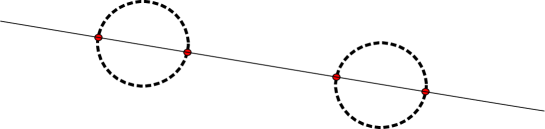
Figure 6. An intersection calculation, reflecting that $w_{2,4}$ pairs non-trivially with $q_{1}*q_{1}$.

Definition 10.3.

Let $w(k,\ell)=w_{2^{k}(2^{\ell}-1),2^{k+\ell}}$.

We will use Corollary 5.4 to show that the Stiefel-Whitney classes $w(k,\ell)$ generate $H^{*}(\coprod_{n}B{\mathcal{S}}_{n})$ as a Hopf ring. The needed calculation is a special case of what is needed to understand the coproducts of these classes, so we treat the entire structure at once.

Proposition 10.4.

Let ${\bf q}$ be a monomial in the $q_{I}$. Then $w_{i,n}$ evaluated on ${\bf q}$ is one if ${\bf q}$ is a product of classes $q_{\ell\cdot 1}$ and $q_{0}$ and is zero otherwise.

Proof.

To set notation $H_{*}(\coprod_{n}BO(n))$ is the free polynomial ring on classes $b_{i}$ in degree $i$, with $i\geq 0$, which are in the homology of $BO(1)={\mathbb{R}}P^{\infty}$. Recall that $w_{i,n}\in H^{i}(BO(n))$ evaluates to one on ${b_{0}}^{n-i}{b_{1}}^{i}$ and to zero on all other classes. This calculation is easily established inductively using the fact that stably the coproduct of $w_{i}$ dual to the Pontrjagin product is $\sum w_{i-j}\otimes w_{j}$.

We use the fact that $\coprod_{n}B\rho_{n}$ is map of $E_{\infty}$-spaces (see for example II.7 of [9]) to see $q_{I}=q_{I}(\iota)$ maps to $q_{I}(b_{0})$. Then we can use the structure of the homology of $\coprod_{n}BO(n)$ over the Kudo-Araki-Dyer-Lashof algebra, as computed by Kochman [15] and then Priddy [22], determined by

(2) $$q_{r}(b_{n})=\sum_{i}\binom{r+i-1}{i}b_{n-i}b_{r+n+i}.$$

Given that $w_{i,n}$ only pairs with ${b_{0}}^{n-i}{b_{1}}^{i}$ we call a monomial $m$, which is product of $b_{j}$’s, tainted if one of those $b_{j}$ has $j>1$. The basic observation is that if $m$ is tainted then $q_{k}(m)$ is tainted for any $k$. Indeed, using the Cartan formula we see that $q_{k}(m)$ is sum of products of $q_{k_{i}}(b_{j_{i}})$. But using Equation 2, for the $j_{i}>1$ the factor $q_{k_{i}}(b_{j_{i}})$ will be a sum of products of two $b$’s of total degree $2j_{i}+k_{i}\geq 4$, so at least one must have degree greater than one.

If in $q_{i_{1},\cdots i_{k}}$ we have $i_{k}>1$, then because $q_{i_{k}}(b_{0})=b_{0}b_{i_{k}}$ is tainted, so will be every term in $q_{i_{1},\cdots i_{k}}(b_{0})$. Thus $w_{i,n}$ must evaluate trivially on any monomial which is a product of at least one such $q_{I}$.

To see that on the other hand $w_{i,n}$ does evaluate non-trivially on a monomial in the $b_{1,\ldots,1}$, we calculate $q_{1,\ldots,1}(b_{0})$. We get that $q_{1}(b_{0})=b_{0}b_{1}$, and then that

$$q_{1,1}(b_{0})=q_{1}(q_{1}(b_{0}))=q_{1}(b_{1}b_{1})=q_{1}(b_{0})q_{0}(b_{1})+q_{0}(b_{0})q_{1}(b_{1})=b_{0}b_{1}^{3}+b_{0}^{3}b_{3}+b_{0}^{2}b_{1}b_{2}.$$

In general, $q_{1,\ldots,1}(b_{0})$ is equal to $b_{0}b_{1}^{2^{k}-1}$ plus tainted monomials. Because $B\rho_{*}$ is a map of rings, a product of such classes in degree $i$ will equal ${b_{0}}^{n-i}{b_{1}}^{i}$ plus tainted monomials, and thus be evaluated non-trivially by $w_{i,n}$, completing the argument. ∎

We now develop the combinatorics necessary to express the coproducts of Stiefel-Whitney classes.

Definition 10.5.

A Dickson bi-partition of the pair $(k,\ell)$ is an equality of pairs of positive integers

$$\left(2^{k}(2^{\ell}-1),2^{k+\ell}\right)=\sum_{i}\left(2^{k_{i}}(2^{\ell_{i}}-1),2^{k_{i}+\ell_{i}}\right).$$

Here we allow the trivial one-term partition, and we allow $k_{i}$ to be zero as well as $\ell_{i}$ to be zero when the corresponding $k_{i}$ is. We manipulate such a partition as a set $p=\{(k_{i},\ell_{i})\}$, and sometimes emphasize the numbers being partitioned by writing $p=p(k,\ell)$.

We say one bi-partition refines another if it is obtained by substituting of some entry or entries by corresponding Dickson bi-partition(s).

For example, because $(24,32)=(4,8)+(6,8)+(14,16)$ we have the corresponding Dickson bi-parition $p(3,2)=\{(2,1),(1,2),(1,3)\}$. Because in turn of the equality $(4,8)=(0,2)+(1,2)+(3,4)$, we have that $q=\{(1,0),(0,1),(1,1),(1,2),(1,3)\}$ refines $p$.

Definition 10.6.

Let $\Pi_{k,\ell}$ denote the set consisting of Dickson bi-partitions $p$ expressed as an ordered union of two smaller partitions $p=p^{\prime}\cup p^{\prime\prime}$, each of which contains no repeated pairs of numbers. Define a partial order on $\Pi_{k,\ell}$ by $p^{\prime}\cup p^{\prime\prime}\leq q^{\prime}\cup q^{\prime\prime}$ if $p^{\prime}$ is a (possibly trivial) refinement of $q^{\prime}$ and $p^{\prime\prime}$ of $q^{\prime\prime}$.

Let $\phi$ be the ${\mathbb{F}}_{2}$-valued function on $\Pi_{k,\ell}$ defined uniquely by

$$\sum_{p^{\prime}\cup p^{\prime\prime}\leq q^{\prime}\cup q^{\prime\prime}}\phi(q^{\prime}\cup q^{\prime\prime})=1,$$

for any $p^{\prime}\cup p^{\prime\prime}\in\Pi_{k,\ell}$.

In other words, the function $\phi$ is the inverse under convolution to the function which is one on all of $\Pi_{k,\ell}$. Thus it could be determined by Möbius inversion, though we have not found that to be enlightening.

Theorem 10.7.

As a Hopf ring, $H^{*}(\coprod_{n}B{\mathcal{S}}_{n})$ is generated by Stiefel-Whitney classes $w(k,\ell)$.

The transfer product is exterior, the antipode is the identity map, and there are no further relations other than those given by Hopf ring distributivity and the fact that the product of classes on different components is zero.

The coproduct is given by

$$\Delta w(k,\ell)=\sum_{p^{\prime}\cup p^{\prime\prime}\in\Pi_{k,\ell}}\phi(p^{\prime}\cup p^{\prime\prime})\left(\bigodot_{(k_{i},\ell_{i})\in p^{\prime}}w(k_{i},\ell_{i})\right)\bigotimes\left(\bigodot_{(k_{j},\ell_{j})\in p^{\prime\prime}}w(k_{j},\ell_{j})\right).$$

Proof.

That these Stiefel-Whitney classes generate is now an immediate application of Proposition 10.4 to verify the hypothesis of Corollary 5.4. The lack of further relations and the additive basis follow from Theorem 5.3 just as this Corollary 5.4 did.

The coproduct formula is verified by direct check using bialgebra structure. By Proposition 10.4, $w(k,\ell)$ evaluated on some non-trivial product $m*m^{\prime}$ which is a monomial will be non-zero if and only if $m$ and $m^{\prime}$ are products of ($q_{0}$’s and) $q_{1,\ldots,1}$’s. Such products are in one-to-one correspondence with the set $\Pi_{k,\ell}$. Looking at only $m$, first we express each ${q_{1,...1}}^{n}$ uniquely as a product of ${q_{1,...,1}}^{2^{k}}=q_{0,.........,0,1,....,1}=q(k,\ell)$, and then record the $(k,\ell)$ which appear. For example, $q_{0}{q_{1}}^{3}{q_{1,1}}{q_{1,1,1}}^{2}=q_{0}*q_{1}*q_{0,1}*q_{1,1}*q_{0,1,1,1}$ corresponds to $\{(1,0),(0,1),(1,1),(0,2),(1,3)\}$. Call this bijection $\beta$ from the set of monomials in $q_{1,...,1}$ to Dickson bi-partitions.

Applying Proposition 10.4, we find that not only does $m\otimes m^{\prime}$ pair with $\bigodot_{(k_{i},\ell_{i})\in\beta(m)}w(k_{i},\ell_{i})\otimes\bigodot_{(k_{j},\ell_{j})\in\beta(m^{\prime})}w(k_{j},\ell_{j})$ but it also pairs with all similar products of Stiefel-Whitney classes over $q^{\prime}\cup q^{\prime\prime}$ which are refined by $\beta(m)\cup\beta(m^{\prime})$. Thus, if we take the linear combination with coefficients given by $\phi$, that sum will pair to one with $m\otimes m^{\prime}$. ∎

References

- [1] John Frank Adams, Infinite loop spaces, Annals of Mathematics Studies, vol. 90, Princeton University Press, Princeton, N.J., 1978. MR 505692 (80d:55001)
- [2] Alejandro Adem, John Maginnis, and R. James Milgram, Symmetric invariants and cohomology of groups, Math. Ann. 287 (1990), no. 3, 391–411. MR 1060683 (91i:55022)
- [3] Alejandro Adem and R. James Milgram, Cohomology of finite groups, Grundlehren der Mathematischen Wissenschaften [Fundamental Principles of Mathematical Sciences], vol. 309, Springer-Verlag, Berlin, 1994. MR MR1317096 (96f:20082)
- [4] José Adem, The relations on Steenrod powers of cohomology classes. Algebraic geometry and topology, A symposium in honor of S. Lefschetz, Princeton University Press, Princeton, N. J., 1957, pp. 191–238. MR MR0085502 (19,50c)
- [5] M. F. Atiyah and G. B. Segal, Equivariant -theory and completion, J. Differential Geometry 3 (1969), 1–18. MR MR0259946 (41 #4575)
- [6] Michael Barratt and Stewart Priddy, On the homology of non-connected monoids and their associated groups, Comment. Math. Helv. 47 (1972), 1–14. MR MR0314940 (47 #3489)
- [7] Terrence P. Bisson and André Joyal, -rings and the homology of the symmetric groups, Operads: Proceedings of Renaissance Conferences (Hartford, CT/Luminy, 1995), Contemp. Math., vol. 202, Amer. Math. Soc., Providence, RI, 1997, pp. 235–286. MR MR1436923 (98e:55021)
- [8] R. R. Bruner, J. P. May, J. E. McClure, and M. Steinberger, ring spectra and their applications, Lecture Notes in Mathematics, vol. 1176, Springer-Verlag, Berlin, 1986. MR MR836132 (88e:55001)
- [9] Frederick R. Cohen, Thomas J. Lada, and J. Peter May, The homology of iterated loop spaces, Springer-Verlag, Berlin, 1976. MR MR0436146 (55 #9096)
- [10] Mark Feshbach, The mod 2 cohomology rings of the symmetric groups and invariants, Topology 41 (2002), no. 1, 57–84. MR MR1871241 (2002h:20074)
- [11] J. H. Gunawardena, J. Lannes, and S. Zarati, Cohomologie des groupes symétriques et application de Quillen, Advances in homotopy theory (Cortona, 1988), London Math. Soc. Lecture Note Ser., vol. 139, Cambridge Univ. Press, Cambridge, 1989, pp. 61–68. MR 1055868 (91d:18013)
- [12] Nguyên H. V. Hung, The action of the Steenrod squares on the modular invariants of linear groups, Proc. Amer. Math. Soc. 113 (1991), no. 4, 1097–1104. MR 1064904 (92c:55018)
- [13] Nguyen Hũ’u Viet Hu’ng, The modulo cohomology algebras of symmetric groups, Japan. J. Math. (N.S.) 13 (1987), no. 1, 169–208. MR MR914318 (89g:55028)
- [14] Donald Knutson, -rings and the representation theory of the symmetric group, Lecture Notes in Mathematics, Vol. 308, Springer-Verlag, Berlin, 1973. MR MR0364425 (51 #679)
- [15] Stanley O. Kochman, Homology of the classical groups over the Dyer-Lashof algebra, Trans. Amer. Math. Soc. 185 (1973), 83–136. MR MR0331386 (48 #9719)
- [16] I. G. Macdonald, Symmetric functions and Hall polynomials, second ed., Oxford Mathematical Monographs, The Clarendon Press Oxford University Press, New York, 1995, With contributions by A. Zelevinsky, Oxford Science Publications. MR 1354144 (96h:05207)
- [17] Ib Madsen and R. James Milgram, The classifying spaces for surgery and cobordism of manifolds, Annals of Mathematics Studies, vol. 92, Princeton University Press, Princeton, N.J., 1979. MR MR548575 (81b:57014)
- [18] R. James Milgram, Private communication.
- [19] by same author, The spherical characteristic classes, Ann. of Math. (2) 92 (1970), 238–261. MR MR0263100 (41 #7705)
- [20] John W. Milnor and John C. Moore, On the structure of Hopf algebras, Ann. of Math. (2) 81 (1965), 211–264. MR MR0174052 (30 #4259)
- [21] Minoru Nakaoka, Homology of the infinite symmetric group, Ann. of Math. (2) 73 (1961), 229–257. MR MR0131874 (24 #A1721)
- [22] Stewart Priddy, Dyer-Lashof operations for the classifying spaces of certain matrix groups, Quart. J. Math. Oxford Ser. (2) 26 (1975), no. 102, 179–193. MR MR0375309 (51 #11505)
- [23] D. G. Quillen, The spectrum of an equivariant cohomology ring, i., Ann. of Math. (2) 94 (1971), 549–572.
- [24] D. G. Quillen and B. B. Venkov, Cohomology of finite groups and elementary abelian subgroups., Topology 11 (1972), 317–318.
- [25] Douglas C. Ravenel and W. Stephen Wilson, The Hopf ring for complex cobordism, J. Pure Appl. Algebra 9 (1976/77), no. 3, 241–280. MR MR0448337 (56 #6644)
- [26] N. E. Steenrod, Homology groups of symmetric groups and reduced power operations, Proc. Nat. Acad. Sci. U. S. A. 39 (1953), 213–217. MR MR0054964 (14,1005d)
- [27] N. P. Strickland, Morava -theory of symmetric groups, Topology 37 (1998), no. 4, 757–779. MR MR1607736 (99e:55008)
- [28] Neil P. Strickland and Paul R. Turner, Rational Morava -theory and , Topology 36 (1997), no. 1, 137–151. MR MR1410468 (97g:55005)
- [29] Andrey V. Zelevinsky, Representations of finite classical groups, Lecture Notes in Mathematics, vol. 869, Springer-Verlag, Berlin, 1981, A Hopf algebra approach. MR MR643482 (83k:20017)