On the Time-Dependent Analysis of Gamow Decay
Robert Grummt

 

Diplomarbeit

München 2009

Fakultät für Physik, Ludwig-Maximilians-Universität München

Abstract

Gamow’s approach to exponential decay of meta-stable particles via complex ’eigenvalues’ (resonances) of a Hamiltonian is scrutinized. We explain the sense in which the non-square-integrable ’eigenfunctions’ that belong to these resonances (Gamow functions) are relevant for the time-evolution of square-integrable wave functions. For concreteness we study a one dimensional square-well potential with a trapping region $K$ and the evolution of wave functions, whose support is initially inside of $K.$ It is shown that the sum over the first few time-evolved Gamow functions restricted to $K$ yields an approximation for the evolution of these initial wave functions within the trapping region. The approximation is good for all times for which exponential decay prevails.
Supervisor: Prof. Dr. Detlef Dürr

Chapter 1 Introduction

The exponential law appearing in connection with the phenomenon of $\alpha$-decay is experimentally well verified. Its quantum mechanical description has a long-standing history and remains the subject of research in mathematical physics to this day. George Gamow [4] was the first to study $\alpha$-decay within non-relativistic Quantum Mechanics in 1928. He considered solutions $G$ to the stationary Schrödinger equation, which correspond to a complex ’eigenvalue’ $\epsilon=E-i\frac{\Gamma}{2}$ rather than a real one. The Schrödinger evolution $G\,e^{-i\epsilon t}$ then immediately implies the exponential decay of the ’Gamow function’ $G$ with decay rate $\Gamma.$ But due to the continuity equation this behavior is only possible when $G$ increases exponentially with increasing $x.$ Therefore, the Gamow function is not square-integrable and has no direct physical relevance. This raises the question whether there is a way to make sense of the Gamow functions. The following argument outlines our approach to the solution of this problem.

The Schrödinger equation is a wave equation. Therefore, potentials whose core is separated from the outside by high barriers will confine wave packets for a long time. This is due to reflection of waves at barriers. Mathematically, this property of the potential becomes manifest in the existence of ’almost bound states’ $G$ or, as we have previously called them, Gamow functions. We already know that they solve

$$(H_{0}+V)\psi=\epsilon\psi$$ (1.1)

with $\epsilon=E-i\frac{\Gamma}{2},$ where the imaginary part will be small due to the long confinement measured by the lifetime $\Gamma^{-1}.$

On the other hand, the time evolution of a wave function $\psi_{0}$ within a potential $V,$ which does not admit any bound states, can be determined by expanding $\psi_{0}$ in so-called generalized eigenfunctions. This yields

$$e^{-iHt}\psi_{0}(x)=\int\hat{\psi}_{0}(k)\phi(k,x)e^{-itk^{2}/2}\,dk,$$ (1.2)

where the eigenfunctions $\phi(k,x)$ are bounded solutions of the stationary Schrödinger equation (1.1) for real $\epsilon=k^{2}/2\geq 0.$ But if the ’eigenvalue’ of the Gamow function is very close to the real axis, the generalized eigenfunction $\phi(\sqrt{2E},x)$ should mimic the shape of $G(x),$ since both functions solve equation (1.1). This argument motivates that

$$\phi(k,x)\sim\eta(k)G(x)$$ (1.3)

for all $k$ in the vicinity of $\sqrt{2E}.$

Clearly, not every initial wave function $\psi_{0}$ will decay exponentially within a certain time regime. But Gamow’s approach suggests that a square-integrable approximation of $G$ yields the exponential law at least within a certain time interval. And a rough approximation is obtained by truncating all of $G$ that lies beyond the core $K$ of the potential, which yields

$$\hat{\psi}_{0}(k)=\int\chi_{{}_{K}}G(x)\overline{\phi(k,x)}\,dx\sim c\,\bar{\eta}(k).$$

Inserting this and relation (1.3) into the integral (1.2), the time evolution of the truncated Gamow function reduces to the Fourier transform of $|\eta(k)|^{2}.$ Therefore, a considerable part of this work is devoted to the properties of the function $\eta.$ It will turn out that, in the vicinity of $\sqrt{2E},$ its squared modulus has Breit-Wigner shape

$$|\eta(k)|^{2}=\frac{|a_{-1}|^{2}}{(k-\mathrm{Re}\ \sqrt{2\epsilon})^{2}+(\mathrm{Im}\ \sqrt{2\epsilon})^{2}}.$$

Since the Fourier transform of the Breit-Wigner distribution is the exponential function, the time evolution of these initial wave functions is then approximately given by

$$e^{-iHt}\psi_{0}(x)\sim c\,G(x)\int|\eta(k)|^{2}e^{-itk^{2}/2}\,dk\sim c\,G(x)e^{-\frac{\Gamma}{2}\,|t|}.$$ (1.4)

Thereby, we have not only found an initial wave function which decays exponentially within a certain time interval, but it also takes the shape of the Gamow function $G.$

Now, this heuristic discussion needs to be turned into a rigorous one. In this regard, the first major step will be taken in Chapter 3, where the precise relation between the generalized eigenfunctions $\phi$ and the Gamow function $G$ will be determined and where $\eta$ will be calculated. This will primarily rely upon the complex continuation of $\phi$ in the variable $k.$ And the second major step will be taken in Chapter 4, where we will understand which initial wave functions $\psi_{0}$ decay exponentially within a certain time regime. The basic technique utilized in the proofs of this chapter is the calculus of residues.

Regarding the question whether Gamow functions have physical relevance, substantial progress was made by Skibsted with [9] and [10]. He also showed that the truncated Gamow function $\chi_{{}_{K}}G$ decays exponentially within a certain time regime. And although expansions in eigenfunctions are used in his approach as well, his proofs do not rely on complex continuation. Nevertheless, he mentions this method as a possible alternative [9, p. 593], even though Skibsted [10, p. 47] considers complex continuation as difficult if rigorous results shall be obtained. However, the author believes that the expansion of $e^{-iHt}\psi_{0}$ in eigenfunctions together with the application of the Residue Theorem to the resulting integral, is the most direct approach to $\alpha$-decay. It clearly demonstrates how exponential decay arises and which role Gamow functions play in this regard. And in spite of the above concerns, we will obtain rigorous results using this method, at least for the specific potential studied in this work. In a sense, this thesis thereby explains the necessity of what was achieved by Skibsted [9]. Moreover, it will complement Skibsted’s work by explaining why truncated Gamow functions are a particularly good choice for proving the exponential decay of $e^{-iHt}\psi_{0}$ within a certain time regime.

Another question that arises in connection with Gamow’s article is, in which sense a self-adjoint operator admits complex ’eigenvalues’ or, as they are customarily called, resonances. In this respect, different definitions of resonances have been studied. The most popular ones are reviewed by Simon [8]. A recent review of Zworski [12] takes the widely accepted definition of resonances, as a pole of the resolvent $(z-H)^{-1}$ for granted. This allows for the study of asymptotic properties of, what could be called, the extended spectrum and the dependence of the resonances on the geometry of configuration space.

However, the main concern of this thesis is to understand the physical relevance of Gamow functions rather than questions regarding the extended spectrum. Therefore, a precise definition of Gamow functions will be provided in the next chapter. This will allow us to study their relation to physically relevant $L^{2}$-functions in the framework of a one dimensional square-well potential. The motivation for choosing this potential was the article [5] of Garrido, Goldstein, Lukkarinen and Tumulka, whose main objective - contrary to this thesis - is to show that an initially localized wave packet leaves the square-well much slower than a classical particle. But before this specific potential is introduced and used to explain why an eigenfunction expansion serves to express $e^{-iHt}\psi_{0}$ as an integral, we will show that square-integrable wave functions generically undergo exponential decay only within a certain time interval. In Chapter 3 we will then establish the precise relation between the generalized eigenfunctions and the Gamow functions for our specific potential. The function $\eta(k),$ which is calculated in this process, is of vital importance for Chapter 4. With its help it will be shown that not only truncated Gamow functions, but also bound states obtained by restricting the original Hamiltonian, decay exponentially within a certain time interval. The bound states will then allow us to extend these results to a general class of initial wave functions. And in this process we will understand why truncated Gamow functions are distinguished initial wave functions. The last chapter will then conclude with an outlook pointing to questions, which remain open.

Notation and Units

The real part of a complex number $z$ will be denoted by $z^{\prime},$ its imaginary part by $z^{\prime\prime}$ and its complex conjugate by $\bar{z}.$ Although, the prime will denote the derivative with respect to a real variable from time to time, it will always be self-evident which meaning of the prime is referred to in the particular context. Moreover, $O(\lambda^{n})$ denotes a function $f(\lambda)$ which is asymptotically of the same order as $\lambda^{n},$ that is

$$\limsup_{\lambda\rightarrow\infty}\left|\frac{f(\lambda)}{\lambda^{n}}\right|<\infty.$$

Apart from this, we choose units in which $\hbar=m=1.$

Chapter 2 Problem and Tools

2.1. Statement of the Problem

To approach the question whether the Gamow functions have physical relevance, we will now define them and rephrase the problem in mathematically precise terms.

Gamow derived the exponential decay law from non-relativistic Quantum Theory, by considering functions $\psi$ that solve the stationary Schrödinger equation

$$-\frac{1}{2}\frac{d^{2}}{dx^{2}}\psi(x)+V(x)\psi(x)=\epsilon\,\psi(x)$$ (2.1)

for complex rather than real $\epsilon.$ Since such a $\psi$ yields the solution

$$\psi(t,\cdot)=e^{-i\epsilon t}\psi(\cdot)$$ (2.2)

to the time dependent Schrödinger equation, it decays exponentially in time when $\mathrm{Im}\ \epsilon$ is negative. But due to the fact that (2.2) needs to respect the continuity equation

$$\partial_{t}|\psi|^{2}+\mathrm{div}\left(\mathrm{Im}\ \bar{\psi}\nabla\psi\right)=0$$

as well, the flux associated to this solution must be outgoing such that both terms on the left hand side cancel. This motivates the following definition of Gamow functions.

Definition 1.

Given the one-dimensional stationary Schrödinger equation (2.1) with a potential $V$ having compact support and non-zero complex $\epsilon$ having negative imaginary part. A function $G\in\mathcal{C}^{1}(\mathbb{R})$ is called Gamow function, if it solves (2.1) and if there is a non-zero constant $C$ such that

$$G(x)=Ce^{+iz|x|}\qquad\forall\,x\in(\text{supp }V)^{c},$$

where $\epsilon=\frac{1}{2}z^{2}=E-i\frac{\Gamma}{2}.$

Thus, Gamow functions are defined by regarding the Schrödinger equation as ordinary differential equation on $\mathcal{C}^{1}$ rather than as an operator identity on a Hilbert space. Since the notion of self-adjointness thereby loses its meaning, it should not be disturbing that the Gamow ’eigenvalue’ $\epsilon$ is complex.

From Definition 1 it becomes evident that Gamow functions do not lie in the Hilbert space $L^{2}(\mathbb{R}).$ For, the negative imaginary part of $z$ directly implies that $G(x)$ must increase exponentially as $|x|$ tends to $\infty.$ Therefore, the question whether the Gamow functions have physical relevance can be rephrased to whether there is a relation between Gamow functions and Hilbert space solutions of the time dependent Schrödinger equation.

As already outlined in the introduction, we will find a relation between $G$ and the generalized eigenfunctions $\phi.$ And although these eigenfunctions do not belong to $L^{2}(\mathbb{R})$ either, they can be used to express the time evolution of a square-integrable wave function $\psi_{0}$ as the integral

$$e^{-iHt}\psi_{0}=\int\hat{\psi}_{0}(k)\phi(k,\cdot)\,dk.$$

And this will allow us to establish a relation between physical relevant Hilbert space solutions of the time dependent Schrödinger equation and Gamow functions.

2.2. Properties of the Schrödinger Evolution

In the current section we will see that $e^{-iHt}\psi$ can not decay exponentially for $t\gg 1$ as well as $t\ll 1.$ This will follow from two well-known properties of the survival probability, which is defined as

$$P_{\psi}(t)=|\left<\psi,e^{-iHt}\psi\right>|^{2}.$$

The proof presented here, is based upon the arguments given by Simon in [8]. And it relies heavily on the spectral theorem for unbounded self-adjoint operators (see e.g. [1, Chapter 2]), such as the Schrödinger operator. Therefore, we will briefly review the contents of this theorem.

Casually speaking, the spectral theorem generalizes the fact that every hermitian matrix can be diagonalized, to operators on Hilbert spaces. To make this precise, let $H$ denote the Schrödinger operator, $\mathcal{H}$ denote the Hilbert space on which it is defined and let $\sigma(H)$ denote its spectrum. Then the spectral theorem guarantees the existence of a finite countably additive measure $\mu$ on $\sigma(H)\times\mathbb{N}$ and the existence of a unitary map

$$\mathcal{F}:\mathcal{H}\rightarrow L^{2}(\sigma(H)\times\mathbb{N},\mu).$$

This map is such that $\mathcal{F}H\mathcal{F}^{-1}=h,$ where $h$ is the multiplication operator associated to the function $h(n,s)=s$ with $s$ being an element of $\sigma(H).$ Since $h$ is the analogue of a diagonal matrix, this justifies the casual statement of the spectral theorem given above. However, $\mathcal{F}$ develops its full power only when it is applied to the operator $f(H)$ with $f$ being an arbitrary bounded measurable function. In this case we find analogously to the identity from above $\mathcal{F}f(H)\mathcal{F}^{-1}=f(h),$ which will be used extensively in the following two proofs. The fact that $\mathcal{F}$ maps onto a direct sum of several $L^{2}(\sigma(H),\mu)$-spaces is due to the devision of $\mathcal{H}$ into cyclic subspaces, which is necessary to prove the spectral theorem. But on every cyclic subspace, $H$ is unitarily equivalent to a multiplication with $h(s).$ Therefore, we will neglect this detail in the sequel without causing any harm.

Having reviewed the spectral theorem, we can now turn to the first of the above-mentioned properties of the survival probability $P_{\psi}.$ It concerns the short time behavior of $e^{-iHt}\psi.$

Lemma 1.

Let $H$ be a self-adjoint operator and let $\psi$ be an element of its domain. Then $P_{\psi}(t)$ is differentiable everywhere and $\dot{P}_{\psi}(0)=0.$

Proof.

The differentiability of $P_{\psi}(t)$ follows from the differentiability of

$$A(t)=\left<\psi,e^{-iHt}\psi\right>.$$

Since $H$ is self-adjoint, the spectral theorem is applicable. This directly implies

$$A(t)=\int_{\sigma(H)}|\mathcal{F}\psi(\epsilon)|^{2}e^{-i\epsilon t}\,\mu(d\epsilon).$$ (2.3)

Using dominated convergence and the inequality of Cauchy-Schwarz, we thereby see that $A$ is differentiable if

$$\bigg{|}\int_{\sigma(H)}\epsilon|\mathcal{F}\psi(\epsilon)|^{2}e^{-i\epsilon t}\,\mu(d\epsilon)\bigg{|}=\left|\left<\psi,e^{-iHt}H\psi\right>\right|\leq\|\psi\|\,\|H\psi\|<\infty.$$

Since this is the case for all $\psi$ in the domain of $H,$ the survival probability $P_{\psi}(t)$ is differentiable for all $t$ in $\mathbb{R}.$

Using the spectral theorem again, $P_{\psi}$ can be rewritten as

$$|\left<\psi,e^{-iHt}\psi\right>|^{2}=\left<\psi,e^{-iHt}\psi\right>\left<\psi,e^{iHt}\psi\right>,$$

which implies that $P_{\psi}(t)=P_{\psi}(-t)$ for all $t$ in $\mathbb{R}$ and $\psi$ in the domain of $H.$ Moreover, an application of the inequality of Cauchy-Schwarz proves that $P_{\psi}(t)\leq P_{\psi}(0).$ From these facts and the differentiability of $P_{\psi},$ we can conclude that $\dot{P}_{\psi}(0)=0.$ ∎

The differentiability of $P_{\psi}$ and the vanishing derivative at zero, immediately imply that

$$P_{\psi}(t)\neq Ce^{-\Gamma t}$$

for small $t.$ So even if $e^{-iHt}\psi$ contains a contribution of the form $e^{-\Gamma t}\tilde{\psi},$ there must be an additive remainder that accounts for the non-exponential behavior of $P_{\psi}$ for small $t.$ Apart from this restriction on the short time behavior of $e^{-iHt}\psi,$ there is another property of the survival probability having implications for the long time behavior.

Lemma 2.

Let $H$ be a self-adjoint operator, whose spectrum is bounded from below. Then the only element $\psi$ in the domain of $H$ that satisfies

$$P_{\psi}(t)\leq Ce^{-\Gamma|t|}$$

for some $C,\Gamma>0$ is the zero element.

Proof.

Since $H$ is self-adjoint and $\psi$ is an element of its domain, equation (2.3) can be utilized again such that

$$A(t)=\int_{\sigma(H)}|\mathcal{F}\psi(\epsilon)|^{2}e^{-i\epsilon t}\,\mu(d\epsilon)=\int_{\mathbb{R}}g(\epsilon)e^{-i\epsilon t}\,\mu(d\epsilon),$$

where $g$ is equal to $|\mathcal{F}\psi|^{2}$ on the spectrum $\sigma(H)$ and zero otherwise. Therefore, $A$ is the Fourier transform of a $L^{1}$-function $g,$ which is supported only on the spectrum of $H.$ By inverting the Fourier transform, we find

$$g(\epsilon)=\int_{\mathbb{R}}A(t)e^{i\epsilon t}\,\mu(dt).$$

And if we assume that

$$|A(t)|\leq Ce^{-\frac{\Gamma}{2}|t|}$$

for some non-zero positive constants $C$ and $\Gamma,$ this formula together with the theorem of dominated convergence implies that $g$ is analytic on the strip $\{\epsilon_{0}+i\eta|\epsilon_{0}\in\mathbb{R},\eta\in(-\Gamma/2,\Gamma/2)\}.$ But the spectrum of $H$ is bounded from below. So $g(\epsilon)$ vanishes for all real $\epsilon$ smaller than the infimum of $\sigma(H).$ Therefore, $g$ must vanish on the whole strip, which is only possible if $\psi$ equals zero. ∎

That there is no exponential bound on $P_{\psi}$, can only be due to the asymptotics of the survival probability and thereby due to the asymptotics of $e^{-iHt}\psi.$ It reflects the fact that the wave function ultimately decays polynomially instead of exponentially. This is not surprising, since it is in accord with the following heuristic scattering theoretical argument (for a detailed discussion see [2, Remark 15.2.4]). The time evolved wave function at the fixed position $x$ is given by

$$e^{-iHt}\psi(x)=t^{-1/2}\int\mathcal{F}\psi\left(\frac{\kappa}{\sqrt{t}}\right)\phi\left(\frac{\kappa}{\sqrt{t}},x\right)e^{-i\frac{\kappa^{2}}{2}}\,d\kappa,$$

where $\kappa/\sqrt{t}$ was substituted for $k.$ In the limit of $t$ tending to $\infty$ the right hand side multiplied by $t^{1/2}$ turns out to be constant, which can be seen heuristically by interchanging limit and integration. For $t\gg 1$ we therefore expect that

$$e^{-iHt}\psi(x)\sim c\,\mathcal{F}\psi(0)\phi(0,x)\,t^{-1/2}.$$

The previous lemmas also show that the heuristic discussion in the introduction, which lead us to

$$e^{-iHt}\psi(x)\sim G(x)\,e^{-\frac{\Gamma}{2}|t|},$$

can only be valid on intermediate time scales. However, for very small as well as very large times the error terms, hidden behind the $\sim$ symbol, will not be negligible anymore. In Chapter 4 this heuristic statement will be turned into a precise one.

Let us conclude this section with the following aside. If exponential decay can prevail on intermediate time scales, we could just choose $t_{0}$ big enough and consider

$$P_{\psi}(t_{0}+t)=|\langle\psi,e^{-iHt}e^{-iHt_{0}}\psi\rangle|^{2}$$

in order to ensure exponential decay even for times $t\ll 1.$ This suggests that by choosing the initial time $t_{0}$ advantageous the result of Lemma 1 can be somehow circumvented. But in fact resetting the initial time results in the quantity

$$|\langle e^{-iHt_{0}}\psi,e^{-iHt}e^{-iHt_{0}}\psi\rangle|^{2}$$

as opposed to $P_{\psi}(t_{0}+t),$ since we really want to compare the time evolved wave function $e^{-iHt}\psi_{t_{0}}$ to the initial wave function $\psi_{t_{0}}.$ And this quantity is identical to $P_{\psi}(t),$ which is why it can not decay exponentially for times $t\ll 1$ either.

2.3. Setting and Tools

The specific potential that provides the framework for this thesis is given by

$$V_{\lambda}(x)=\lambda\chi_{[-a,a]}(x)\quad\text{with}\quad a,\lambda>0$$ (2.4)

and is illustrated in Figure 2.1. Due to the reflection of waves at barriers, it confines initially localized wave packets for a long time if $\lambda\gg 1.$ As was already mentioned in the introduction, $V_{\lambda}$ will therefore admit resonances. Since it is explicitly solvable too, $V_{\lambda}$ is a good choice for approaching the question whether Gamow functions have physical relevance.

Figure 2.1. Plot of the potential $V_{\lambda}.$

Clearly, the function $V_{\lambda}(x)$ defines a multiplication operator $V_{\lambda}$ acting on $L^{2}(\mathbb{R}).$ It is not difficult to see that this operator is symmetric and bounded. And in particular, $V_{\lambda}$ has relative bound zero with respect to the free Schrödinger operator $H_{0}$ acting on $L^{2}(\mathbb{R}).$ The Kato-Rellich theorem (see [1, Theorem 1.4.2]) therefore immediately implies that $H_{\lambda}=H_{0}+V_{\lambda}$ is self-adjoint with domain $H^{2}(\mathbb{R})=\mathcal{D}(H_{0}).$ And due to the self-adjointness, the spectral theorem guarantees the existence of a map $\mathcal{F}$ yielding the spectral representation of $H_{\lambda}.$ In the previous section we already used this map, in order to diagonalize $e^{-iHt}.$ Regarding the time evolution of the wave function $\psi_{0},$ this only yields

$$e^{-iH_{\lambda}t}\psi_{0}=\mathcal{F}^{-1}e^{-i(\cdot)t}\mathcal{F}\psi_{0}.$$

In order to get any further we need to determine $\mathcal{F}$ explicitly. Fortunately, for our simple potential this can be done. One possibility to achieve $\mathcal{F},$ is to determine the integral kernel of the resolvent $(z-H_{\lambda})^{-1}$ which rather directly yields the spectral measure $dP_{\epsilon}.$ This strategy is pursued in [11, Chapter 23] to which we refer for details. However, after doing the calculations one will find that the map $\mathcal{F}$ yielding the spectral representation of $H_{\lambda}$ can be defined as an integral operator

$$\mathcal{F}\psi(k)=\int_{\mathbb{R}}\psi(x)\overline{\phi(k,x)}dx$$ (2.5)

with respect to the Lebesgue measure. And the integral kernel turns out to be an element of $L^{\infty},$ which solves

$$-\frac{1}{2}\frac{d^{2}}{dx^{2}}\phi(k,x)+V\phi(k,x)=\epsilon\,\phi(k,x)\quad\text{for}\quad\epsilon=\frac{k^{2}}{2}\geq 0$$ (2.6)

and is therefore called generalized eigenfunction. Although, bona fide eigenfunctions usually enter into the explicit expression of $\mathcal{F}$ as well, this is not the case for $V_{\lambda}.$ For this particular potential the pure point spectrum is empty. Thus, there are no bona fide eigenfunctions and the spectrum is given by

$$\sigma(H_{\lambda})=[0,\infty).$$

Before we continue, notice the similarity of equation (2.5) with the Fourier transform. It has earned $\mathcal{F}$ the name generalized Fourier transform. Clearly, the generalized eigenfunctions $\phi$ define the spectral representation of the perturbed Hamiltonian $H_{\lambda}$ in complete analogy to the way the plane waves $e^{ikx}$ define the spectral representation of $H_{0}.$ And it is often helpful to remember this analogy.

2.4. Resonances and Gamow Functions

In the present section we will determine the Gamow functions that belong to the potential $V_{\lambda}.$ Thereby, we will not only have an explicit example for their generic definition. But in the process of calculating the Gamow functions, we will also determine the approximate location of the corresponding ’eigenvalues’. Although these eigenvalues will be called resonances from now on, it will only be seen in the next chapter that their defining equation coincides with the formula which defines the poles of the $S$-Matrix thereby justifying this name.

An ansatz for the solution of equation (2.1) with potential $V_{\lambda},$ which satisfies the boundary conditions of Definition 1 is given by

$$G(x)=\begin{cases}Ae^{-izx}\quad\quad&,x<-a\\ Be^{i\tilde{z}x}+Ce^{-i\tilde{z}x}&,|x|\leq a\\ De^{izx}&,x>a\end{cases}$$

$$\text{with}\quad\tilde{z}=\sqrt{z^{2}-2\lambda}.$$

Whereas the complex square root is defined such that $\mathrm{Re}\ \sqrt{w}>0$ for all $w$ in $\mathbb{C}\setminus(-\infty,0].$ So whenever $\mathrm{Im}\ w\lessgtr 0$ we know that $\mathrm{Im}\ \sqrt{w}\lessgtr 0.$ For $G$ to be an element of $\mathcal{C}^{1}$ as required from the definition of Gamow functions, its first derivative and itself have to be continuous at $x$ equal to $\pm a$. This will be the case when the coefficients satisfy the following homogeneous system of linear equations

$$\begin{pmatrix}e^{iza}&-e^{-i\tilde{z}a}&-e^{i\tilde{z}a}&0\\ -ize^{iza}&-i\tilde{z}e^{-i\tilde{z}a}&i\tilde{z}e^{i\tilde{z}a}&0\\ 0&-e^{i\tilde{z}a}&-e^{-i\tilde{z}a}&e^{iza}\\ 0&-i\tilde{z}e^{i\tilde{z}a}&i\tilde{z}e^{-i\tilde{z}a}&ize^{iza}\end{pmatrix}\begin{pmatrix}A\\ B\\ C\\ D\end{pmatrix}=0.$$ (2.7)

Due to the fact that this system has non-trivial solutions only when the determinant of the matrix vanishes, the equation

$$e^{i4a\tilde{z}}=\left(\frac{z+\tilde{z}}{z-\tilde{z}}\right)^{2}$$ (2.8)

needs to have solutions for Gamow functions to exist.

Lemma 3.

Given the potential $V_{\lambda}$ with fixed width $a>0,$ there is a Gamow function corresponding to every integer $n$ which satisfies

$$1\leq n<\frac{2}{\pi}\sqrt{2a^{2}\lambda-1}.$$ (2.9)

Moreover, if such an $n$ is fixed the corresponding resonance is given by

$$z_{n}=\left(2\lambda+\frac{n^{2}\pi^{2}}{4a^{2}}\right)^{1/2}-i\frac{n^{2}\pi^{2}}{4a^{3}\sqrt{2\lambda}}\left(2\lambda+\frac{n^{2}\pi^{2}}{4a^{2}}\right)^{-1/2}+O(\lambda^{-3/2})\quad\text{and}$$

$$\tilde{z}_{n}=\frac{n\pi}{2a}-i\frac{n\pi}{2a^{2}\sqrt{2\lambda}}+O(\lambda^{-1})$$

respectively.

Proof.

Due to the fact that $\exp(-in2\pi)=1$ for all $n$ in $\mathbb{Z},$ the identity (2.8) represents a whole family of equations numbered by the integer $n.$ Using the definition of $\tilde{z},$ this family can be expressed as

$$e^{i4a\sqrt{2\lambda}\tilde{\kappa}-in2\pi}=\left(\tilde{\kappa}+\sqrt{\tilde{\kappa}^{2}+1}\right)^{4},$$

where $\tilde{\kappa}$ denotes $\tilde{z}/\sqrt{2\lambda}.$ And with the help of some simple manipulations we can even bring it into the fixed-point form

$$F_{n}(\tilde{\kappa}):=n\frac{\pi}{2a\sqrt{2\lambda}}-i\frac{1}{a\sqrt{2\lambda}}\ln(\tilde{\kappa}+\sqrt{\tilde{\kappa}^{2}+1})=\tilde{\kappa},$$

where $\ln$ denotes the principal branch of the complex logarithm. Therefore, the Banach Fixed Point Theorem (see [3, Chapter 9.2.1]) can be applied to each of these equations in order to find their solutions by iteration.

This theorem is applicable whenever $F_{n}$ is contractive on a closed subset $T$ of $\mathbb{C}$ and $T$ is invariant under $F_{n}.$ Due to the fact that the derivative of $F_{n}$ satisfies

$$|F_{n}^{\prime}|=\frac{1}{a\sqrt{2\lambda}}\frac{1}{|1+\tilde{\kappa}^{2}|^{1/2}}\leq\frac{1}{a\sqrt{2\lambda}}\frac{1}{|1-|\tilde{\kappa}|^{2}|^{1/2}},$$

the map is contractive on $T=\{\tilde{\kappa}\in\mathbb{C}\big{|}|\tilde{\kappa}|\leq K\}$ with $K$ being a constant which satisfies

$$0<K<\sqrt{1-\frac{1}{2a^{2}\lambda}}.$$

The requirement of having an invariant subset will restrict $K$ further. In order for $|F_{n}(\tilde{\kappa})|\leq K$ to hold, we need

$$|F_{n}(\tilde{\kappa})|\leq|F_{n}(\tilde{\kappa})-F_{n}(0)|+|F_{n}(0)|\leq\frac{1}{a\sqrt{2\lambda}}\frac{|\tilde{\kappa}|}{|1-|\tilde{\kappa}|^{2}|^{1/2}}+|n|\frac{\pi}{2a\sqrt{2\lambda}}\leq K.$$

But since every term is positive, this can only be the case for non-zero $\tilde{\kappa},$ if

$$|n|\frac{\pi}{2a\sqrt{2\lambda}}<K.$$

Together with the upper bound on $K$ from above, we thereby conclude that

$$1+\left(\frac{n\pi}{2}\right)^{2}<2a^{2}\lambda$$ (2.10)

needs to hold true for such a $K$ to exist. Thus, for fixed parameters $a$ and $\lambda$ the Banach Fixed Point Theorem can only be applied to those fixed-point equations whose index satisfies (2.10). If the parameters are such that this inequality is fulfilled, $n=0$ will always be allowed. But the corresponding fixed-point equation has $\tilde{\kappa}=0$ as its unique solution, which leads us to the trivial solution of the Schrödinger equation. Since this was excluded in the definition of Gamow functions, we require $|n|\geq 1.$

To prove the second part of the Lemma let $a>0$ be fixed, assume that $\lambda$ is big enough for (2.9) to allow resonances and fix an $n$ which satisfies this condition. Then we can iterate the corresponding fixed-point equation in order to find the location of the $n$th resonance. If this is done up to second order starting with $\tilde{\kappa}^{(0)}=0,$ we end up with a rather cumbersome expression. Expanding this expression in powers of $\lambda^{-1/2}$ and keeping only the first non-vanishing order of real and imaginary part yields

$$\tilde{\kappa}^{(2)}_{n}=\frac{n\pi}{2a\sqrt{2\lambda}}-i\frac{n\pi}{4a^{2}\lambda}+O(\lambda^{-3/2})\quad\text{and}\quad\tilde{z}_{n}=\frac{n\pi}{2a}-i\frac{n\pi}{2a^{2}\sqrt{2\lambda}}+O(\lambda^{-1})$$

respectively. If we use the definition of $\tilde{z}$ and expand again we also get

$$z_{n}=(\tilde{z}_{n}^{2}+2\lambda)^{1/2}=\left(2\lambda+\frac{n^{2}\pi^{2}}{4a^{2}}\right)^{1/2}-i\frac{n^{2}\pi^{2}}{4a^{3}\sqrt{2\lambda}}\left(2\lambda+\frac{n^{2}\pi^{2}}{4a^{2}}\right)^{-1/2}+O(\lambda^{-3/2}),$$

where we implicitly used that $\mathrm{Im}\ \sqrt{z}<0$ whenever $\mathrm{Im}\ z<0.$ And in order for $\mathrm{Im}\ \tilde{z}_{n}$ to be negative, $n$ is restricted to positive integers. ∎

To determine the Gamow functions that correspond to the resonances just found in the previous lemma, it remains to solve the homogeneous system of linear equations (2.7). A series of straightforward calculations yields

$$G(x)=B\begin{cases}\frac{2\tilde{z}}{\tilde{z}-z}e^{-i\tilde{z}a}e^{-iz(x+a)}&,x<-a\\ \\ e^{i\tilde{z}x}+\frac{\tilde{z}-z}{\tilde{z}+z}e^{i\tilde{z}a}e^{-i\tilde{z}(x-a)}&,|x|\leq a\\ \\ \frac{2\tilde{z}}{\tilde{z}+z}e^{i\tilde{z}a}e^{iz(x-a)}&,x>a.\end{cases}$$

Evaluating this expression at $z=z_{n}$ immediately implies that

$$G_{n}(x)=\begin{cases}\frac{\tilde{z}_{n}}{\tilde{z}_{n}+z_{n}}e^{i\tilde{z}_{n}a}e^{-iz_{n}(x+a)}&,x<-a\\ \\ \cos\tilde{z}_{n}x&,|x|\leq a\\ \\ \frac{\tilde{z}_{n}}{\tilde{z}_{n}+z_{n}}e^{i\tilde{z}_{n}a}e^{iz_{n}(x-a)}&,x>a\end{cases}$$ (2.11)

for odd $n,$ while

$$G_{n}(x)=\begin{cases}-\frac{\tilde{z}_{n}}{\tilde{z}_{n}+z_{n}}e^{i\tilde{z}_{n}a}e^{-iz_{n}(x+a)}&,x<-a\\ \\ i\sin\tilde{z}_{n}x&,|x|\leq a\\ \\ \frac{\tilde{z}_{n}}{\tilde{z}_{n}+z_{n}}e^{i\tilde{z}_{n}a}e^{iz_{n}(x-a)}&,x>a\end{cases}$$ (2.12)

for even $n,$ where $B$ was set to $1/2.$ This can be seen by using

$$e^{i2\tilde{z}_{n}a}\frac{\tilde{z}_{n}-z_{n}}{\tilde{z}_{n}+z_{n}}=\begin{cases}+1\quad,n\text{ odd}\\ -1\quad,n\text{ even},\end{cases}$$

which directly follows from equation (2.8) with $-in2\pi$ added to the exponent on the left hand side.

We conclude this chapter with Figure 2.2, which illustrates that the Gamow functions do indeed increase exponentially in $x.$ In the next chapter we will establish a connection between these functions and the generalized eigenfunctions. For this purpose, the explicit expression for the resonances will become relevant again, since we will discover that the generalized eigenfunctions have poles located at the resonances.

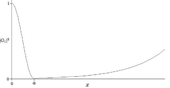
Figure 2.2. Plot of the squared modulus $|G_{1}|^{2}$ of the Gamow function corresponding to the first resonance with parameter choice $a=2$ and $\lambda=30.$ Notice that for $x>a$ the function is strongly compressed in the $x$-direction, to make the exponential increase better visible. This was done by inserting the factor $\lambda$ in front of $(x-a).$

Chapter 3 Generalized Eigenfunctions and Strategy

In this chapter we will establish precisely how the Gamow functions are connected with the generalized eigenfunctions of the potential $V_{\lambda}.$ Thereby, the relation

$$\phi(k,x)\sim\eta(k)G(x)$$

that was announced in the introduction will be turned into a rigorous statement, from which the function $\eta$ will be deduced. But the major part of this chapter is devoted to the properties of $\eta$ that are needed to prove the exponential decay of truncated Gamow functions within a certain time regime.

3.1. Calculation of the Eigenfunctions

First of all, the generalized eigenfunctions that belong to the potential $V_{\lambda}$ will be calculated. Clearly, there are symmetric and anti-symmetric solutions to a symmetrical potential and considering both cases separately simplifies calculations considerably. An ansatz for the symmetric generalized eigenfunctions is given by

$$\phi(k,x)=\begin{cases}Ae^{ikx}+Be^{-ikx}\quad&,x<-a\\ C(e^{i\tilde{k}x}+e^{-i\tilde{k}x})&,|x|\leq a\\ Be^{ikx}+Ae^{-ikx}&,x>a,\end{cases}$$

where $\tilde{k}=\sqrt{k^{2}-2\lambda}$. Due to the symmetry condition, it is sufficient to require that $\phi$ and its first derivative are continuous at $x$ equal to $+a$ in order to guarantee continuity everywhere. And this yields the following homogeneous system of linear equations

$$Ae^{-ika}+Be^{ika}-C(e^{i\tilde{k}a}+e^{-i\tilde{k}a}) =0$$

$$-Ae^{-ika}+Be^{ika}-\frac{\tilde{k}}{k}C(e^{i\tilde{k}a}-e^{-i\tilde{k}a}) =0.$$

Upon solving this system, the symmetric generalized eigenfunctions are given by

$$\phi(k,x)=Ae^{-ika}\begin{cases}e^{ik(x+a)}+\frac{\bar{F}(k)}{F(k)}e^{-ik(x+a)}\quad&,x<-a\\ \\ \frac{2}{F(k)}\cos\tilde{k}x&,|x|\leq a\\ \\ e^{-ik(x-a)}+\frac{\bar{F}(k)}{F(k)}e^{ik(x-a)}&,x>a\end{cases}$$ (3.1)

$$\text{with}\quad F(k)=\cos\tilde{k}a-i\frac{\tilde{k}}{k}\sin\tilde{k}a.$$

Since this is a $L^{\infty}$-solution to the Schrödinger equation, it can not be normalized in the usual $L^{2}$-sense. But similarly to the usual Fourier transform it is required that $\int\overline{\phi(k^{\prime},x)}\phi(k,x)\,dx=\delta(k^{\prime}-k).$ And this gives $A=\frac{1}{\sqrt{4\pi}}$.

Analogously the ansatz for the anti-symmetric generalized eigenfunctions leads to the following expression

$$\phi(k,x)=\frac{e^{-ika}}{\sqrt{4\pi}}\begin{cases}e^{ik(x+a)}-\frac{\bar{J}(k)}{J(k)}e^{-ik(x+a)}\quad&,x<-a\\ \\ \frac{2i}{J(k)}\sin\tilde{k}x&,|x|\leq a\\ \\ -e^{-ik(x-a)}+\frac{\bar{J}(k)}{J(k)}e^{ik(x-a)}&,x>a\end{cases}$$ (3.2)

$$\text{with}\quad J(k)=\frac{\tilde{k}}{k}\cos\tilde{k}a-i\sin\tilde{k}a.$$

3.2. Refined Strategy

The purpose of this section is to refine the argument that served to illustrate in the introduction how the exponential decay of $e^{-iHt}\psi_{0}$ arises within a certain time regime.

A vital part of this argument was the relation $\phi(k,x)\sim\eta(k)G(x).$ But given that the generalized eigenfunctions solve $(\epsilon-H_{0})\phi=V\phi$ their generic structure is

$$\phi(k,x)=e^{ikx}+\Phi(k,x),$$ (3.3)

that is general solution to the homogeneous part plus particular solution to the inhomogeneous part. And usually it is not the $\Phi(k,x)$ part that governs the time evolution

$$e^{-iHt}\psi_{0}(x)=\int\mathcal{F}\psi_{0}(k)\phi(k,x)e^{-i\frac{k^{2}}{2}t}\,dk,$$ (3.4)

but the $e^{ikx}$ part. However, only $\Phi$ can cause the generalized eigenfunctions to mimic the shape of the Gamow function $G.$ Therefore, we are interested in the situation in which this function gives the dominating contribution to the generalized eigenfunctions. And heuristically this will be the case when

$$|\Phi(k,x)|=|\phi(k,x)-e^{ikx}|\gg|e^{ikx}|.$$

Clearly, the generalized eigenfunctions that belong to $V_{\lambda}$ have the structure (3.3). And according to the above-mentioned argument, we expect that they take the shape of $G$ when

$$|F|^{-1}\gg 1\quad\text{and}\quad|J|^{-1}\gg 1$$

respectively. In fact, the squared modulus of $F^{-1}$ consists of a series of Breit-Wigner distributions whose height is of $O(\lambda).$ This is illustrated in Figure 3.1 and will be proven rigorously later. Since these distributions are represented by the formula

$$\frac{|a_{-1}|^{2}}{(k-z^{\prime}_{n})^{2}+z^{\prime\prime 2}_{n}}=\frac{|a_{-1}|^{2}}{(k-z^{\prime}_{n}-iz^{\prime\prime}_{n})(k-z^{\prime}_{n}+iz^{\prime\prime}_{n})},$$

their appearance in $|F|^{-2}$ reflects the fact that the continuation of $\phi(k,x)$ to the complex $k$-plane has poles due to $F^{-1}.$ Therefore, we just need to apply the calculus of residues to the above-mentioned integral (3.4) to extract a term being proportional to $\exp(-z^{\prime}_{n}z^{\prime\prime}_{n}\,t).$ So for those $t$ for which this term gives the dominating contribution to $e^{-iH_{\lambda}t}\psi_{0},$ the wave function will decay exponentially. But before we pursue this idea further, the existence of the poles will be proven in the next lemma.

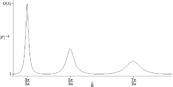
Figure 3.1. Plot of $|F|^{-2}$ with parameter choice $a=2$ and $\lambda=100,$ where $kF(k)$ denotes the Jost function of the symmetric generalized eigenfunctions. The $k$-axis was rescaled by using the relation $\tilde{k}=\sqrt{k^{2}-2\lambda}.$

Lemma 4.

The complex continuations of $F$ and $J$ have roots, which coincide with the resonances $z_{n}$ corresponding to odd $n$ and even $n$ respectively. In both cases the multiplicity of the roots is one.

Proof.

As already noted in Section 2.4, the resonances $z_{n}$ satisfy the following identity

$$e^{i2a\tilde{z}_{n}}\,\frac{\tilde{z}_{n}-z_{n}}{\tilde{z}_{n}+z_{n}}=\begin{cases}+1\quad,n\text{ odd}\\ -1\quad,n\text{ even}.\end{cases}$$

Using this, a straightforward calculation shows that

$$\frac{e^{ia\tilde{z}_{n}}-e^{-ia\tilde{z}_{n}}}{e^{ia\tilde{z}_{n}}+e^{-ia\tilde{z}_{n}}}=\frac{z_{n}}{\tilde{z}_{n}}$$

holds for odd $n.$ And it is not difficult to see that this equation is equivalent to $\tan\tilde{z}_{n}a=-i\frac{z_{n}}{\tilde{z}_{n}},$ which is the equation satisfied by the roots of $F.$ An analogous argumentation holds for $J$ with even $n.$

To show that the multiplicity of the roots is one, we need to show that $F^{\prime}(z_{2n-1})$ and $J^{\prime}(z_{2n})$ do not vanish. In this regard, notice that

$$F^{\prime}(z_{2n-1})=-ia\left(\cos\tilde{k}a-i\frac{k}{\tilde{k}}\sin\tilde{k}a\right)-i\frac{2\lambda}{\tilde{k}k^{2}}\sin\tilde{k}a\bigg{|}_{k=z_{2n-1}}.$$

Using the fact that $F(z_{2n-1})=0,$ this can be expressed as

$$F^{\prime}(z_{2n-1})=-\left(a-\frac{i}{k}\right)\frac{2\lambda}{\tilde{k}k}\sin\tilde{k}a\bigg{|}_{k=z_{2n-1}}.$$

The term in brackets can not vanish, because $\mathrm{Re}\ z_{2n-1}$ is non-zero. Since the sine has roots only on the real axis and $\mathrm{Im}\ z_{2n-1}>0,$ it can not vanish either. Hence, $F^{\prime}(z_{2n-1})$ is non-zero. An analogous argumentation holds for $J.$ ∎

According to the previous lemma, the poles of the generalized eigenfunctions coincide with the resonances, which justifies that the Gamow ’eigenvalues’ have been termed this way. In order to see this notice that $kF(k)$ and $kJ(k)$ are so called Jost functions (see [9, Section 2]), which define the Scattering-Matrix by

$$S(k)=\frac{\bar{F}(k)}{F(k)}\quad\text{and}\quad S(k)=\frac{\bar{J}(k)}{J(k)}$$

respectively. Since it is common to define resonances as poles of the complex continuation of this operator, we see that they coincide with the roots of $F$ and $J$ and thereby with the Gamow ’eigenvalues’. Although, this was only verified for $V_{\lambda},$ Skibsted’s article [9] shows that it remains true for more general potentials.

Another consequence of this observation, is that the Gamow function $G_{n}$ and the residue of $\phi(k,\cdot)$ at $z_{n}$ are linearly dependent. In order to see this let $\varphi$ be defined by

$$\phi(k,\cdot)=\frac{\varphi(k,\cdot)}{H(k)},$$

where $H$ denotes either $F$ or $J$. Then $\mathrm{Res}\,\,\phi=a_{-1}\,\varphi(z_{n},\cdot).$ And given that the Jost function evaluated at $z_{n}$ can be expressed as (see [9, Section 2])

$$z_{n}H(z_{n})=\begin{vmatrix}G_{n}(x)&\varphi(z_{n},x)\\ \frac{d}{dx}G_{n}(x)&\frac{d}{dx}\varphi(z_{n},x)\end{vmatrix},$$

the linear dependence becomes immediately evident, when we recall that $H(z_{n})=0.$ Therefore, we can establish a precise relation between the generalized eigenfunctions and the Gamow functions by expanding $\phi$ in a Laurent series about the resonance $z_{n}.$ This yields the expression

$$\phi(k,x)=\underbrace{\frac{a_{-1}}{k-z_{n}}\,c}_{\eta(k)}\,G_{n}(x)+\text{Remainder},$$

from which $\eta(k)$ can be simply read off.

3.3. Laurent Expansion of the Eigenfunctions

This section will show that for big enough $\lambda$ there is an interval $[z^{\prime}_{n}-\delta,z^{\prime}_{n}+\delta]$ on which the principal part $\eta(k)G$ of the Laurent expansion of $\phi(k,\cdot)$ is a good approximation for the generalized eigenfunctions. In the next chapter this will allow us to justify the approximation

$$e^{-iH_{\lambda}t}\psi_{0}=\int\mathcal{F}\psi_{0}(k)\phi(k,\cdot)e^{-i\frac{k^{2}}{2}t}\,dk\sim G(\cdot)\,\int\mathcal{F}\psi_{0}(k)\eta(k)e^{-i\frac{k^{2}}{2}t}\,dk$$

for those initial wave functions, whose energy distribution $\mathcal{F}\psi_{0}$ is concentrated in the above-mentioned interval.

Due to the fact that $V_{\lambda}$ has compact support, the generalized eigenfunctions break up in a part being valid on the support of $V_{\lambda}$ and a part being valid on its complement. Therefore, it is convenient to consider the time evolution integral (3.4) on these subsets of $\mathbb{R}$ separately. For now, we focus on $supp\,\,V_{\lambda}.$ And this will require frequent use of the characteristic function $\chi_{{}_{[-a,a]}},$ which is why it is advantageous to introduce the following shorthand

$$\chi_{a}:=\chi_{{}_{[-a,a]}}.$$

Moreover, it is convenient to restrict ourselves to symmetric initial wave functions such that only the symmetric generalized eigenfunctions (3.1) contribute to the integral (3.4). However, every result has a straightforward extension to the anti-symmetric case.

Lemma 5.

Let $\phi$ denote the symmetric generalized eigenfunctions of $H_{\lambda}$ with $\lambda\in\mathbb{R}^{+}$ and let $z_{2n-1}$ with $n\geq 1$ denote its resonances. Then $\phi$ can be expanded in the Laurent series

$$\phi(k,x)=e^{-ika}\left(\frac{a_{-1}(x)}{k-z_{2n-1}}+a_{0}(x)+R_{0}(k,x)\right),$$ (3.5)

for every $x$ in $[-a,a].$ And if $\lambda$ is chosen big enough, there is a $\delta>0,$ such that this expansion converges absolutely and uniformly on $[z^{\prime}_{2n-1}-\delta,z^{\prime}_{2n-1}+\delta],$ provided $n$ satisfies

$$1\leq n<\sqrt{\frac{\lambda}{2}-\sqrt{2\lambda}}=:n_{\lambda}.$$

Proof.

In Lemma 4 it was proven that the resonances $z_{2n-1}$ are first order poles of the complex continuation of $\phi(k,x)$ to the lower complex $k$ plane. Thus, it is clear that the Laurent expansion of $\phi$ is given by (3.5). In order to prove that it converges in the above-mentioned interval about $z^{\prime}_{2n-1},$ we will determine its annulus of convergence. Since the resonances are separated points in the complex plane, it is clear that it will be a punctured disc around that particular resonance $z_{2n-1}.$ So it remains to estimate the outer radius of convergence, which can be done by estimating the distance between neighboring poles of $\phi.$

By Lemma 4, the symmetric generalized eigenfunctions have poles numbered by odd indices, while the anti-symmetric ones have poles numbered by even indices. Therefore, we need to ensure that

$$|z_{2n+1}-z_{2n-1}|^{2}>4z^{\prime\prime 2}_{2n+1}>4z^{\prime\prime 2}_{2n-1}\qquad\text{for }n\geq 1,$$ (3.6)

where the last inequality will automatically hold if the first one is true. This is due to $z^{\prime\prime 2}_{k}$ being a monotonically increasing function of $k.$ Notice, that the factor in front of the imaginary part is chosen for convenience, but is not optimal. Using the explicit formula for the resonances given in Lemma 3, we find

$$|z_{2n+1}-z_{2n-1}|^{2} =\left(\sqrt{2\lambda+\frac{(2n+1)^{2}\pi^{2}}{4a^{2}}}-\sqrt{2\lambda+\frac{(2n-1)^{2}\pi^{2}}{4a^{2}}}\right)^{2}$$

$$\qquad+\frac{\pi^{2}}{4a^{2}}\frac{1}{2\lambda}\left(\frac{2n+1}{\left(1+\frac{4a^{2}\,2\lambda}{(2n+1)^{2}\pi^{2}}\right)^{1/2}}-\frac{2n-1}{\left(1+\frac{4a^{2}\,2\lambda}{(2n-1)^{2}\pi^{2}}\right)^{1/2}}\right)^{2}.$$

By exploiting the formula $(a+b)(a-b)=a^{2}-b^{2},$ the term in brackets appearing in the first summand can be simplified to

$$\frac{\pi^{2}}{4a^{2}}\frac{8n}{\sqrt{2\lambda+\frac{(2n+1)^{2}\pi^{2}}{4a^{2}}}+\sqrt{2\lambda+\frac{(2n-1)^{2}\pi^{2}}{4a^{2}}}}\geq\frac{\pi^{2}}{4a^{2}}\frac{8n}{2\sqrt{2\lambda+\frac{(2n+1)^{2}\pi^{2}}{4a^{2}}}}.$$

The second summand can be simplified by using a similar argumentation, which yields the following lower bound

$$\frac{\pi^{2}}{4a^{2}}\frac{1}{2\lambda}\left(\frac{2}{\left(1+\frac{4a^{2}\,2\lambda}{(2n+1)^{2}\pi^{2}}\right)^{1/2}}\right)^{2}=\left(\frac{\pi^{2}}{4a^{2}}\right)^{2}\frac{1}{2\lambda}\,\frac{4(2n+1)^{2}}{2\lambda+\frac{(2n+1)^{2}\pi^{2}}{4a^{2}}}.$$

Together these lower bounds imply that inequality (3.6) is full filled, if

$$\left(\frac{\pi^{2}}{4a^{2}}\right)^{2}\frac{(4n)^{2}+\frac{1}{2\lambda}4(2n+1)^{2}}{2\lambda+\frac{(2n+1)^{2}\pi^{2}}{4a^{2}}}>4z^{\prime\prime 2}_{2n+1}=\left(\frac{\pi^{2}}{4a^{2}}\right)^{2}\frac{1}{2\lambda}\frac{4(2n+1)^{4}}{2\lambda+\frac{(2n+1)^{2}\pi^{2}}{4a^{2}}}.$$

Hence, inequality (3.6) holds if

$$(4n)^{2}>\frac{2}{\lambda}(2n+1)^{2}((2n+1)^{2}-1).$$

Some simple rearrangements and estimates yield the following inequality

$$0>n^{2}-\left(\frac{\sqrt{2\lambda}}{2}-1\right)n+\frac{1}{4},$$

where equality would hold for

$$n_{\pm}=\frac{1}{2}\left(\left(\frac{\sqrt{2\lambda}}{2}-1\right)\pm\sqrt{\left(\frac{\sqrt{2\lambda}}{2}-1\right)^{2}-1}\right).$$

Clearly, $n_{-}$ will approach zero in the limit of $\lambda$ tending to $\infty.$ Therefore, only $n_{+}$ is of relevance when $\lambda\gg 1$ and $n\geq 1.$ And if we regard $n_{+}$ as arithmetic mean, this allows us to conclude that the distance $|z_{2n+1}-z_{2n-1}|$ between neighboring resonances is larger than $2|z^{\prime\prime}_{2n+1}|$ for all integer $n,$ which satisfy

$$1\leq n<\sqrt{\frac{\lambda}{2}-\sqrt{2\lambda}}=:n_{\lambda}.$$

So for these resonances there is a non-zero positive $\delta,$ such that the Laurent expansion (3.5) converges absolutely and uniformly for all $k$ in $[z^{\prime}_{n}-\delta,z^{\prime}_{n}+\delta].$ ∎

That the region in which the Laurent expansion (3.5) converges ceases to intersect the real axis is not surprising. It reflects the fact that the influence of the resonances fades the larger their real part grows. From a physical point of view this can be anticipated, since initial wave functions with high energy $\left<\psi_{0},H_{\lambda}\psi_{0}\right>$ impinge on the ’barrier’ with increased rate. Thus, their lifetime on top of the plateau is reduced.

But more importantly, Lemma 5 shows that

$$\eta_{n}(k)=e^{-ika}\frac{a_{-1}}{k-z_{2n-1}}\quad\text{with}\quad a_{-1}=\underset{z_{2n-1}}{Res}\left(\frac{1}{\sqrt{\pi}F(k)}\right),$$

which verifies the Breit-Wigner shape of $|\eta_{n}|^{2}$ as announced in the introduction.

The estimates on the remainder of the Laurent expansion, will involve contour integrals around circles in the complex $k$-plane. But to handle them some properties of the corresponding contour performed by $\tilde{k}=\sqrt{k^{2}-2\lambda}$ are needed. And the relevant details will be established in the following lemma by considering the function $\sqrt{c+d\,e^{i\varphi}},$ where $0\leq d\leq c$ are real constants. Basically, this function will perform a contour which looks like an egg whose symmetry axis coincides with the real axis. This becomes plausible by rewriting the argument of the complex square root in polar form $r(\varphi)\,\exp(iS(\varphi)).$ Then the effect of the square root on the exponential is to compress the circle in the direction of the imaginary axis, whereas its effect on the radius $r(\varphi)$ shifts its center and will cause the circle to be compressed along the real axis. Since the strength of these effects depends on $\varphi,$ the resulting contour will roughly look like an egg. For the purpose of estimating the remainder, the only information we need is in which region of the complex $k$-plane the contour performed by $\tilde{k}$ can be found. And the preceding illustration suggests that it is an annulus. The following lemma makes this precise.

Lemma 6.

Let $0\leq d\leq c$ be real and let $\varphi$ lie in $[0,2\pi).$ Then the complex contour $\sqrt{c+d\,e^{i\varphi}},$ remains within the annulus $S$ enclosed by the circles

$$z_{out} =\sqrt{c}+r_{out}\,e^{i\varphi}\text{ with }r_{out}=\sqrt{c}-\sqrt{c-d}\text{ and}$$

$$z_{in} =\sqrt{c}+r_{in}\,e^{i\varphi}\text{ with }r_{in}=\sqrt{c+d}-\sqrt{c}.$$

Proof.

The assertion follows, if we show that the continuous function $f(\varphi)$ defined by $|\sqrt{c+d\,e^{i\varphi}}-\sqrt{c}|$ remains within the interval $[r_{in},r_{out}].$ This can be done by showing that $f^{2}$ takes its only maximum at $\varphi$ being equal to $\pi$ and its only minimum at $\varphi$ being equal to zero. In order to do that, it is enough to show that $f^{2}$ is monotonically increasing on the interval $(0,\pi),$ while it is monotonically decreasing on $(\pi,2\pi).$

The monotonicity can be deduced from the sign of the first derivative of $f^{2}.$ But this will be easier if $f^{2}$ is rewritten first. By using the equality $(a+b)(a-b)=a^{2}-b^{2},$ we see that

$$f^{2}(\varphi)=\frac{d^{2}}{|\sqrt{c+d\,e^{i\varphi}}+\sqrt{c}|^{2}},$$

which has the following derivative with respect to $\varphi$

$$-\frac{d^{2}}{|\sqrt{c+d\,e^{i\varphi}}+\sqrt{c}|^{4}}\partial_{\varphi}|\underbrace{\sqrt{c+d\,e^{i\varphi}}+\sqrt{c}|^{2}}_{=:\tilde{f}^{2}}.$$

That means, $f^{2}$ is increasing whenever $\tilde{f}^{2}$ is decreasing and vice versa. In order to determine which of these cases occurs for which $\varphi,$ we need to carry out the differentiation of $\tilde{f}^{2}$ symbolically

$$\partial_{\varphi}\tilde{f}^{2} =2\,(\mathrm{Re}\ \sqrt{c+d\,e^{i\varphi}}+\sqrt{c})\,\partial_{\varphi}\mathrm{Re}\ \sqrt{c+d\,e^{i\varphi}}$$

$$\qquad+2\,\mathrm{Im}\ \sqrt{c+d\,e^{i\varphi}}\,\partial_{\varphi}\mathrm{Im}\ \sqrt{c+d\,e^{i\varphi}}.$$

With the help of the formula $\sqrt{x+iy}=2^{-1/2}\left((\sqrt{x^{2}+y^{2}}+x)^{1/2}+i\,\text{sgn}(y)(\sqrt{x^{2}+y^{2}}-x)^{1/2}\right),$ which is easily proved by rewriting the argument of the square root in polar form, we can bring real and imaginary part in the following form

$$\mathrm{Re}\ \sqrt{c+d\,e^{i\varphi}} =\frac{1}{\sqrt{2}}\left(\sqrt{c^{2}+d^{2}+2cd\cos\varphi}+c+d\cos\varphi\right)^{1/2}\text{ and}$$

$$\mathrm{Im}\ \sqrt{c+d\,e^{i\varphi}} =\text{sgn}(\sin\varphi)\frac{1}{\sqrt{2}}\left(\sqrt{c^{2}+d^{2}+2cd\cos\varphi}-(c+d\cos\varphi)\right)^{1/2}.$$

Using these formulas, the real and imaginary part can be differentiated with respect to $\varphi,$ yielding

$$\partial_{\varphi}\mathrm{Re}\ \sqrt{c+d\,e^{i\varphi}} =\frac{1}{4}\frac{1}{\mathrm{Re}\ \sqrt{c+d\,e^{i\varphi}}}\left(\frac{-cd\sin\varphi}{\sqrt{c^{2}+d^{2}+2cd\cos\varphi}}-d\sin\varphi\right)\text{ and}$$

$$\partial_{\varphi}\mathrm{Im}\ \sqrt{c+d\,e^{i\varphi}} =\frac{1}{4}\frac{\text{sgn}(\sin\varphi)}{\mathrm{Im}\ \sqrt{c+d\,e^{i\varphi}}}\left(\frac{-cd\sin\varphi}{\sqrt{c^{2}+d^{2}+2cd\cos\varphi}}+d\sin\varphi\right).$$

Therefore, we arrive at the following expression for the derivative of $\tilde{f}^{2}$

$$\partial_{\varphi}\tilde{f}^{2} =-\frac{d\sin\varphi}{2}\left(\frac{c}{\sqrt{c^{2}+d^{2}+2cd\cos\varphi}}+1\right)\left(1+\frac{\sqrt{c}}{\mathrm{Re}\ \sqrt{c+d\,e^{i\varphi}}}\right)$$

$$\quad+\frac{d\sin\varphi}{2}\left(\frac{-c}{\sqrt{c^{2}+d^{2}+2cd\cos\varphi}}+1\right)\text{sgn}(\sin\varphi)$$

$$=g(\varphi)+h(\varphi).$$

Comparing both summands factor by factor, we see that $|g|$ is strictly bigger than $|h|$ on the interval $(0,\pi)$ and $(\pi,2\pi).$ And the signs of $g$ and $h$ are such that $f^{2}$ is monotonically increasing in the first case, while it is monotonically decreasing on $(\pi,2\pi).$ Therefore, $f^{2}$ reaches its maximum at $\pi$ and its minimum at zero. So if we define

$$r_{out} =f(\pi)=\sqrt{c}-\sqrt{c-d}\text{ and}$$

$$r_{in} =f(0)=\sqrt{c+d}-\sqrt{c},$$

we can conclude that the contour performed by $\sqrt{c+d\,e^{i\varphi}}$ remains within the annulus $S,$ which is enclosed by the circles with radii $r_{in}$ and $r_{out}$ both being centered at $\sqrt{c}.$ ∎

We can now estimate the modulus of the remainder of the Laurent expansion.

Theorem 1.

Let $\phi$ denote the symmetric generalized eigenfunctions of $H_{\lambda}$ and let $n$ be a fixed odd integer satisfying $1\leq n<n_{\lambda}.$ If $\lambda$ is chosen big enough, the Laurent expansion of $e^{ika}\phi(k,\cdot)$ in $k$ about the resonance $z_{n}$ converges for all $k$ in $[z^{\prime}_{n}-\delta,z^{\prime}_{n}+\delta]$ with

$$\delta=\frac{1}{2}(z^{\prime}_{n}-z^{\prime}_{n-1}).$$

Furthermore, the Laurent coefficients $a_{m}(\cdot)$ and the remainder $R_{0}(k,\cdot)$ satisfy

$$\|\chi_{a}a_{m}(\cdot)\|_{\infty}\leq O(\lambda^{m/2})\text{ and}$$

$$\|\chi_{a}R_{0}(k,\cdot)\|_{\infty}\leq O(\lambda^{1/2})|k-z_{n}|.$$

Proof.

The $L^{\infty}$ bounds on the coefficients will be proven first. Since (3.5) is a Laurent expansion its coefficients can be calculated by

$$a_{m}(\cdot)=\frac{1}{2\pi i}\oint_{C}\frac{\phi(z,\cdot)e^{iza}}{(z-z_{n})^{m+1}}\,dz,$$

where $C$ is a closed contour around the pole $z_{n},$ which remains within the annulus of convergence. Using the explicit form of the generalized eigenfunctions given in (3.1), we therefore have the following upper bound

$$\|\chi_{a}a_{m}(\cdot)\|_{\infty}\leq\frac{1}{\sqrt{\pi}}\sup_{z\in C}\frac{1}{|\cos a\tilde{z}-i\frac{\tilde{z}}{z}\sin a\tilde{z}|}\,\sup_{z\in C}\,\sup_{x\in\mathbb{R}}|\chi_{a}\cos\tilde{z}x|\,\,\,r^{-m}.$$ (3.7)

Here $C$ was chosen to be the circle

$$\{z_{n}+re^{i\varphi}\,|\,\varphi\in[0,2\pi)\}\text{ with}$$ (3.8)

$$r=z^{\prime}_{n}-z^{\prime}_{n-1},$$

which is a contour within the annulus of convergence for all $n,$ since only one pole is enclosed. To handle the suprema appearing in (3.7), we need to know how the circle $C$ in the $z$ plane looks like in the $\tilde{z}$ plane. Due to the fact that we are only interested in the limit of $\lambda$ tending to $\infty,$ we can exploit the dependence of $z_{n}$ on $\lambda$ in order to find

$$\tilde{z}=(z^{2}-2\lambda)^{1/2} =(z_{n}^{2}-2\lambda+2z_{n}re^{i\varphi}+r^{2}e^{i2\varphi})^{1/2}$$

$$=(\tilde{z}^{\prime 2}_{n}+2(z^{\prime}_{n}+iz^{\prime\prime}_{n})re^{i\varphi})^{1/2}$$

$$=\left(\tilde{z}^{\prime 2}_{n}+2z^{\prime}_{n}\sqrt{2\lambda}\left(1+\frac{1}{2}\frac{(2n-1)^{2}\pi^{2}}{4a^{2}2\lambda}-1-\frac{1}{2}\frac{(2n-2)^{2}\pi^{2}}{4a^{2}2\lambda}\right)e^{i\varphi}\right)^{1/2}$$

$$=(\tilde{z}^{\prime 2}_{n}+(\tilde{z}^{\prime 2}_{n}-\tilde{z}^{\prime 2}_{n-1})e^{i\varphi})^{1/2}=:\sqrt{\tilde{z}^{{}^{\prime}2}_{n}+r^{\prime}e^{i\varphi}},$$

which does not depend on $\lambda$ anymore. Thus,

$$\sup_{z\in C}\sup_{x\in\mathbb{R}}|\chi_{a}\cos\tilde{z}x|\leq\sup_{z\in C}\,\sup_{x\in\mathbb{R}}\,\chi_{a}\cosh{\tilde{z}^{\prime\prime}x}=\sup_{z\in C}\,\cosh{\tilde{z}^{\prime\prime}a}\leq c,$$ (3.9)

since $\tilde{z}^{\prime\prime}$ is independent of $\lambda$ on the circle $C.$ And for similar reasons

$$\frac{|\tilde{z}|}{|z|}|\sin a\tilde{z}|\leq\frac{c}{|z|}=O(\lambda^{-1/2}),$$

from which we can deduce

$$\sup_{z\in C}\frac{1}{|\cos a\tilde{z}-i\frac{\tilde{z}}{z}\sin a\tilde{z}|} \leq\left(\inf_{z\in C}|\cos a\tilde{z}|-|\frac{\tilde{z}}{z}\sin a\tilde{z}|\right)^{-1}\leq\left(\inf_{z\in C}|\cos a\tilde{z}|-\frac{1}{4}\right)^{-1},$$

provided $\lambda$ is big enough. So it remains to estimate the infimum of $|\cos a\tilde{z}|$ on the circle $C.$ Regarding this, the information given in Lemma 6 will be sufficient, due to the maximum modulus principle of complex analysis (see e.g. [6]). According to this principle, the modulus of an analytic non-constant function considered on a connected open subset $S$ of $\mathbb{C},$ reaches its maximum on the boundary $\partial S.$ Lemma 6 proves that the contour $C$ remains within the annulus $S$ bounded by the circles

$$\tilde{z}_{in} =\tilde{z}^{\prime}_{n}+\left(\sqrt{2\tilde{z}^{\prime 2}_{n}-\tilde{z}^{\prime 2}_{n-1}}-\tilde{z}^{\prime}_{n}\right)\,e^{i\varphi}\text{ and}$$

$$\tilde{z}_{out} =\tilde{z}^{\prime}_{n}+(\tilde{z}^{\prime}_{n}-\tilde{z}^{\prime}_{n-1})\,e^{i\varphi}.$$

Since these circles enclose exactly one root of $\cos a\tilde{z}$ at their center, $(\cos a\tilde{z})^{-1}$ is analytic within the annulus $S.$ Thus the maximum modulus principle is applicable and it can be concluded that $|\cos a\tilde{z}|$ reaches its minimum on one of the circles $\tilde{z}_{in}$ or $\tilde{z}_{out}.$

In order to find the minimum of $|\cos a\tilde{z}|$ on the above mentioned circles, it is easiest to consider the squared modulus. Since $a\tilde{z}^{\prime}_{n}$ is a root of the cosine, the squared modulus can be rewritten as follows

$$|\cos(a\tilde{z}^{\prime}_{n}+are^{i\varphi})|^{2}=|\sin(are^{i\varphi})|^{2}=\frac{1}{2}(\cosh(2ar\sin\varphi)-\cos(2ar\cos\varphi)),$$

where $r$ denotes either $r_{in}$ or $r_{out}.$ Due to the symmetry of this expression about $\pi,$ it is enough to consider

$$\partial_{\varphi}|\sin(are^{i\varphi})|^{2}=ar(\sinh(2ar\sin\varphi)\cos\varphi-\sin(2ar\cos\varphi)\sin\varphi)$$

on the interval $[0,\pi].$ For $\varphi$ in $(0,\pi/2)$ we also know that $\cos\varphi$ and thereby the first summand is positive. In this case

$$\partial_{\varphi}|\sin(are^{i\varphi})|^{2}\geq ar\sin\varphi(2ar\cos\varphi-\sin(2ar\cos\varphi))>0,$$

since $\sinh x$ is bigger than $x$ and $(x-\sin x)$ is bigger than zero for all positive $x.$ However, should $\varphi$ lie in $(\pi/2,\pi)$ we know that $\cos\varphi$ is negative. Then

$$\partial_{\varphi}|\sin(are^{i\varphi})|^{2} =-ar(\sinh(-2ar\sin\varphi)\cos\varphi-\sin(-2ar\cos\varphi)\sin\varphi)$$

$$\leq-ar\sin\varphi((-2ar\cos\varphi)-\sin(-2ar\cos\varphi))<0$$

for the same reasons as above. The monotonicity implied by these considerations shows that $|\sin(are^{i\varphi})|^{2}$ reaches its minima at zero and $\pi.$ But due to symmetry the modulus of this function at zero will not differ from its modulus at $\pi,$ which is why

$$\inf_{z\in C}|\cos a\tilde{z}|\geq\inf_{z\in S}|\cos a\tilde{z}|=\min\left\{|\cos a\tilde{z}_{in}(0)|,|\cos a\tilde{z}_{out}(0)|\right\}.$$

A lower bound for this minimum can be found by determining lower bounds for the cosines. Since $\tilde{z}_{in}(0)=\sqrt{2\tilde{z}^{\prime 2}_{n}-\tilde{z}^{\prime 2}_{n-1}},$ we see that

$$|\cos(a\tilde{z}_{in}(0))|^{2}=\frac{1}{2}\left(1+\cos\left(2a\sqrt{2\tilde{z}^{\prime 2}_{n}-\tilde{z}^{\prime 2}_{n-1}}\right)\right)=\frac{1}{2}\left(1+\cos\left(2n\pi\sqrt{1-\frac{1}{2n^{2}}}\right)\right),$$

where the explicit location of the resonances $\tilde{z}_{n}$ was used. Considering the square root in the argument of the remaining cosine as deviation from $2n\pi,$ where the cosine would take its maximum, it becomes clear that

$$|\cos(a\tilde{z}_{in}(0))|^{2}\overset{n=1}{\geq}\frac{1}{2}(1+\cos(\sqrt{2}\pi))\geq\frac{1}{2}\left(1+\cos\left(\frac{5}{4}\pi\right)\right)=\frac{1}{2}\left(1-\frac{1}{\sqrt{2}}\right).$$

Using the explicit location of the resonances $\tilde{z}_{n}$ again, we also find

$$|\cos(a\tilde{z}_{out}(0))|^{2}=|\cos(n\pi)|^{2}=1.$$

And this immediately implies that

$$\inf_{z\in C}|\cos a\tilde{z}|\geq\sqrt{\frac{1}{2}\left(1-\frac{1}{\sqrt{2}}\right)}>\frac{1}{3},$$

from which we can conclude

$$\sup_{z\in C}\frac{1}{|\cos a\tilde{z}-i\frac{\tilde{z}}{z}\sin a\tilde{z}|}\leq\left(\inf_{z\in C}|\cos a\tilde{z}|-\frac{1}{4}\right)^{-1}\leq 12$$

provided $\lambda$ is big enough.

This was the missing estimate for the upper bound of the $L^{\infty}$-norm of the Laurent coefficients $\chi_{a}a_{m}(\cdot).$ Using this inequality together with inequality (3.9), we can deduce from the usual Cauchy estimate (3.7) for the Laurent coefficients that

$$\|\chi_{a}a_{m}(\cdot)\|_{\infty}\leq cr^{-m} =c(z^{\prime}_{n}-z^{\prime}_{n-1})^{-m}=O(\lambda^{m/2}).$$

It remains to prove the bound on the remainder $R_{0}$ of the Laurent expansion. Multiplying (3.5) by $e^{ika}$ and subtracting the principal part of the Laurent expansion on both sides yields

$$e^{ika}\phi(k,x)-\frac{a_{-1}(x)}{k-z_{n}}=a_{0}(x)+R_{0}(k,x).$$

Since the right hand side is a Taylor expansion of the left hand side in the complex variable $k,$ the Lagrange form of the remainder can be used, to get an upper bound on the modulus of $R_{0}.$ (Notice that, the Lagrange form of the remainder only gives a bound in dimensions bigger than one, but it is not exact anymore.) So if $k$ is within the radius of convergence of the Taylor series, there is a

$$\zeta\in\{z_{n}+t(k-z_{n})|t\in(0,1)\}\quad\text{such that}$$

$$\|\chi_{a}R_{0}(k,\cdot)\|_{\infty}\leq\left\|\chi_{a}\partial_{k}[e^{ika}\phi(k,\cdot)](\zeta)\right\|_{\infty}\,|k-z_{n}|,$$

where we exploited that the $a_{m}$ are equal to the Laurent coefficients of $e^{ika}\phi(k,\cdot).$ Using Cauchy’s formula, the derivative that appears in the above bound can be estimated as follows

$$\|\chi_{a}\partial_{k}[e^{ika}\phi(k,\cdot)](\zeta)\|_{\infty} =\frac{1}{2\pi}\left\|\chi_{a}\oint_{C}\frac{e^{iza}\phi(z,\cdot)}{(z-\zeta)^{2}}\,dz\right\|_{\infty}$$

$$\leq\frac{1}{2\pi}\sup_{z\in C}\sup_{x\in\mathbb{R}}|\chi_{a}e^{iza}\phi(z,x)|\,\oint_{C}\frac{1}{|z-\zeta|^{2}}\,dz,$$

where $C$ needs to be a closed contour that contains $\zeta.$ The supremum can be estimated as above, when the domain of $\zeta$ is contained in the interior of the circle (3.8), provided $C$ is chosen to be this contour. If we postpone proving that $\zeta$ satisfies this condition, we can conclude that the supremum of $\|\chi_{a}e^{iza}\phi(z,\cdot)\|_{\infty}$ over all $z\in C$ is of $O(\lambda^{0}).$ And this together with the particular form of the contour $C,$ implies

$$\|\chi_{a}\partial_{k}[e^{ika}\phi(k,\cdot)](\zeta)\|_{\infty} \leq\frac{O(\lambda^{0})}{2\pi}r\int_{0}^{2\pi}\frac{1}{|z_{n}-\zeta+re^{i\varphi}|^{2}}\,d\varphi$$

$$\leq O(\lambda^{0})\,r\left(\inf_{\varphi\in[0,2\pi)}|z_{n}-\zeta+re^{i\varphi}|^{2}\right)^{-1},$$

where $r$ denotes $(z^{\prime}_{n}-z^{\prime}_{n-1}).$ The term in brackets can be estimated as follows

$$|z_{n}-\zeta+re^{i\varphi}|^{2}=|w+re^{i\varphi}|^{2} =(w^{\prime}+r\cos\varphi)^{2}+(w^{\prime\prime}+r\sin\varphi)^{2}$$

$$\geq(|w^{\prime}|-r)^{2}+(|w^{\prime\prime}|-r)^{2}$$

$$\geq 2r(r-(|w^{\prime}|+|w^{\prime\prime}|)).$$

Since $k$ is in $[z^{\prime}_{n}-\delta,z^{\prime}_{n}+\delta]$ with $\delta$ being equal to $\frac{1}{2}(z^{\prime}_{n}-z^{\prime}_{n-1}),$ the real part of $\zeta$ will lie in the very same interval, which implies

$$|w+re^{i\varphi}|^{2}\geq r(z^{\prime}_{n}-z^{\prime}_{n-1}-2|w^{\prime\prime}|)\geq r(r-2|z^{\prime\prime}_{n}|)=r\,O(\lambda^{-1/2}).$$

Thus, we can conclude that

$$\|\chi_{a}R_{0}(k,\cdot)\|_{\infty}\leq O(\lambda^{1/2})|k-z_{n}|\qquad\forall\,k\in[z^{\prime}_{n}-\delta,z^{\prime}_{n}+\delta],$$

provided $\lambda$ is big enough. So it remains to show that the domain of $\zeta$ is contained in the interior of the circle defined by (3.8). This is the case if

$$|k-z_{n}|^{2}<(z^{\prime}_{n}-z^{\prime}_{n-1})^{2}\qquad\forall\,k\in[z^{\prime}_{n}-\delta,z^{\prime}_{n}+\delta].$$

But on this interval

$$|k-z_{n}|^{2}\leq\delta^{2}+z^{\prime\prime 2}_{n}=\frac{1}{4}r^{2}+z^{\prime\prime 2}_{n}.$$

So for fixed $n,$ the variable $\zeta$ will lie in the interior of the circle (3.8), if

$$z^{\prime\prime 2}_{n}<\frac{3}{4}r^{2}=O(\lambda^{-1}).$$

For big enough $\lambda$ this condition is full filled, since $z^{\prime\prime 2}_{n}$ is of $O(\lambda^{-2}).$ Notice that $r$ is smaller than $|z_{n}-z_{n-2}|.$ Hence, this condition will also ensure that the $k$ interval of interest, will lie within the annulus on which the Laurent expansion of $\phi$ converges. ∎

Chapter 4 Exponential Decay

The purpose of this chapter is to show that the truncated Gamow functions $\chi_{a}G_{n}$ decay exponentially within a certain time regime on the support of $V_{\lambda}.$ Thereby, the last step of the heuristic discussion given in the introduction, which is

$$e^{-iHt}\psi_{0}(x)\sim\int\mathcal{F}\psi_{0}(k)\eta(k)G(x)e^{-i\frac{k^{2}}{2}t}\,dk\sim G(x)\,e^{-\frac{\Gamma}{2}\,t},$$ (4.1)

will be turned into a precise statement. We will discover that the error which is produced by this approximation decreases with increasing $\lambda.$ And after we have determined the regime in which the exponential law is valid, we will conclude by extending these results to initial wave functions which lie in $\mathcal{C}^{2}([-a,a])$ and vanish at $\pm a.$

4.1. Truncated Gamow Functions

The exponential decay of the truncated Gamow functions $\chi_{a}G_{n}$ within a certain time regime follows from the exponential decay of any other initial wave function lying in their neighborhood (with respect to the $L^{2}$-norm). This is due to the unitarity of $e^{-iH_{\lambda}t},$ which implies that an $L^{2}$-neighbor $\psi_{n}$ of the truncated Gamow function $\chi_{a}G_{n}$ satisfies

$$\|e^{-iH_{\lambda}t}\chi_{a}G_{n}-e^{-iH_{\lambda}t}\psi_{n}\|_{2}=\|\chi_{a}G_{n}-\psi_{n}\|_{2}\ll 1.$$

So for now it will make no difference if we choose the bound states of $H_{\lambda}$ restrictedto $L_{D}=\{\psi\in L^{2}([-a,a])|\psi(a)=\psi(-a)=0\}$ in place of $\chi_{a}G_{n}.$ But we will benefit from this choice when the results derived for these specific initial wave functions will be extended to generic ones. Apart from that, we restrict ourselves to symmetric bound states for convenience, and in order to see that they lie in the vicinity of $\chi_{a}G_{n},$ notice that the symmetric bound states are given by

$$\psi_{n}=\cos(\tilde{z}^{\prime}_{2n-1}\,\cdot)\chi_{a}.$$

Therefore, they differ from the symmetric truncated Gamow functions only by the appearance of the real part $\tilde{z}^{\prime}_{2n-1}$ instead of the entire resonance $\tilde{z}_{2n-1}.$ Given that the imaginary part of the resonance is of $O(\lambda^{-1/2})$ we only need to choose $\lambda$ big enough to ensure that the distance between the symmetric bound states and the symmetric truncated Gamow functions is small enough with respect to the $L^{2}$-norm.

In order to show that the time evolved symmetric bound states decay exponentially within a certain time regime, we need to determine $e^{-iH_{\lambda}t}\psi_{n}.$ In this regard, we will exploit that for big $\lambda$ the major part of the $L^{2}$-mass of the energy distribution $\mathcal{F}\psi_{n}(k)$ is concentrated in a small interval about $z^{\prime}_{2n-1}.$ This becomes evident from

$$\mathcal{F}\psi_{n}(k)=\hat{\psi}_{n}(k)=\frac{c_{n}\,e^{ika}}{\bar{F}(k)}\,\frac{\cos\tilde{k}a}{z^{{}^{\prime}2}_{2n-1}-k^{2}}\,.$$ (4.2)

Its second factor resembles a $\mathrm{sinc}$-function which is peaked about $z^{\prime}_{2n-1}$ and has roots at $z^{\prime}_{2m-1}$ for all $m\neq n.$ Due to the fact that $|\bar{F}(z^{\prime}_{2m})|^{-1}$ is of $O(\lambda^{0})$ and $|\bar{F}(z^{\prime}_{2m-1})|^{-1}$ is of $O(\lambda^{1/2})$ for all integer $m,$ this causes $|\hat{\psi}_{n}|$ to be strongly peaked in a neighborhood of $z^{\prime}_{2n-1}$ while being of $O(\lambda^{0})$ everywhere else. And since the distance between neighboring roots of the energy distribution is of $O(\lambda^{-1/2}),$ we conclude that the major part of the $L^{2}$-mass of $\hat{\psi}_{n}$ is concentrated in the interval

$$[z^{\prime}_{2n-1}-\delta,z^{\prime}_{2n-1}+\delta]\quad\text{with}\quad\delta=\frac{1}{2}(z^{\prime}_{2n-1}-z^{\prime}_{2n-2})=O(\lambda^{-1/2}).$$ (4.3)

This property of the energy distribution $\hat{\psi}_{n}$ is the reason why the time evolution of the symmetric bound states is governed by the generalized eigenfunctions $\phi(k,\cdot)$ that belong to the interval (4.3). So this property is the reason for (4.1) to be a good approximation. However, for the rigorous justification of (4.1) we need to estimate the error that is produced when $\phi(k,\cdot)$ is replaced by $\eta_{n}(k)G_{n},$ which is its leading order contribution on the interval (4.3). Therefore, we will consider

$$\chi_{a}e^{-iH_{\lambda}t}\psi_{n} =\chi_{a}\int_{0}^{\infty}\hat{\psi}_{n}(k)\eta_{n}(k)G_{n}(\cdot)e^{-i\frac{k^{2}}{2}t}\,dk$$

$$\quad+\chi_{a}\int_{0}^{\infty}\hat{\psi}_{n}(k)(\phi(k,\cdot)-\eta_{n}(k)G_{n}(\cdot))e^{-i\frac{k^{2}}{2}t}\,dk$$

and prove that the $L^{2}$-norm of the error integral

$$E_{n}(\cdot,t)=\chi_{a}\int_{0}^{\infty}\hat{\psi}_{n}(k)(\phi(k,\cdot)-\eta_{n}(k)G_{n}(\cdot))e^{-i\frac{k^{2}}{2}t}\,dk$$

is small, while we will see that its main contribution

$$\Psi_{n}(\cdot,t)=\chi_{a}\int_{0}^{\infty}\hat{\psi}_{n}(k)\eta_{n}(k)G_{n}(\cdot)e^{-i\frac{k^{2}}{2}t}\,dk$$

decays exponentially within a certain time regime.

4.2. Truncated Gamow Functions - Main Contribution

In the current section it will be shown that the main contribution $\Psi_{n}$ to $\chi_{a}e^{-iH_{\lambda}t}\psi_{n}$ decays exponentially within a certain time regime and moreover this regime will be determined.

In order to prove that there is a time interval in which

$$\Psi_{n}(\cdot,t)=\chi_{a}G_{n}\int_{0}^{\infty}\hat{\psi}_{n}(k)\,e^{-ika}\,\frac{a_{-1}}{k-z_{2n-1}}e^{-i\frac{k^{2}}{2}t}\,dk$$

decays exponentially, we will use the calculus of residues. Due to the term $\exp(-i\frac{k^{2}}{2}t),$ the integration contour needs to run through the lower complex $k$-plane in order to get converging integrals. In particular, we will choose the contour illustrated in Figure 4.1 with $R$ tending to $\infty,$ which results in an exponentially decaying contribution to $\Psi_{n}$ caused by the pole of $\eta_{n}.$ Therefore, our main task will be to determine the contribution from the rest of the integration contour and to show that it can be neglected during a certain time regime.

Figure 4.1. Illustration of the integration contour $C$ in the complex $k$-plane, where $R$ is understood to tend to $\infty.$

Lemma 7.

Let $n$ be a fixed odd integer satisfying $1\leq n<n_{\lambda}.$ Then for all $t>0,$ we have

$$\Psi_{n}(\cdot,t)=c\,\chi_{a}G_{n}e^{-i\frac{z^{2}_{n}}{2}t}+\chi_{a}G_{n}r(t),$$ (4.4)

where the non-zero constant $c$ is of $O(\lambda^{0})$ and

$$|r(t)|\leq O(\lambda^{-2})\,t^{-1/2}.$$

Proof.

By the residue theorem

$$\oint_{C}\hat{\psi}_{n}(z)\eta_{n}(z)e^{-i\frac{z^{2}}{2}t}\,dz=-2\pi i\,\underset{z_{n}}{Res}\left(\hat{\psi}_{n}\eta_{n}e^{-i\frac{t}{2}(\cdot)^{2}}\right),$$

where $C$ is the contour illustrated in Figure 4.1. From this figure it becomes clear that the contour integral breaks up into

$$\int_{0}^{\infty}\hat{\psi}_{n}(k)\eta_{n}(k)e^{-i\frac{k^{2}}{2}t}\,dk+\int_{C_{1}+C_{2}}\hat{\psi}_{n}(z)\eta_{n}(z)e^{-i\frac{z^{2}}{2}t}\,dz.$$

We will show first that the arc-like part $C_{1}$ of the integration contour gives no contribution. In this respect, notice that

$$|\int_{C_{1}}|\leq\lim_{R\rightarrow\infty}R\int_{0}^{\pi/4}|\hat{\psi}_{n}(Re^{-i\varphi})\eta_{n}(Re^{-i\varphi})|\,e^{-\frac{t}{2}R^{2}\sin 2\varphi}\,d\varphi.$$

As $\lim_{R\rightarrow\infty}|\hat{\psi}_{n}(Re^{-i\varphi})e^{-iaRe^{-i\varphi}}|=0$ for all $\varphi$ in $[0,\pi/4],$ which becomes evident by a straightforward calculation, we only need to choose $R$ big enough to ensure the following estimates

$$|\int_{C_{1}}| \leq\lim_{R\rightarrow\infty}cR\int_{0}^{\pi/4}((R\cos\varphi-z^{\prime}_{n})^{2}+(R\sin\varphi+z^{\prime\prime}_{n})^{2})^{-1/2}\,e^{-\frac{t}{2}R^{2}\sin 2\varphi}\,d\varphi$$

$$\leq\lim_{R\rightarrow\infty}cR\int_{0}^{\pi/4}|R\cos\varphi-\frac{R}{2}\cos\varphi|^{-1}\,e^{-\frac{t}{2}R^{2}\frac{2}{\pi}\varphi}\,d\varphi$$

$$\leq\lim_{R\rightarrow\infty}c^{\prime}\int_{0}^{\pi/4}e^{-\frac{t}{2}R^{2}\frac{2}{\pi}\varphi}\,d\varphi=\lim_{R\rightarrow\infty}c^{\prime\prime}\left(\frac{1-e^{-t\frac{R^{2}}{4}}}{tR^{2}}\right)=0.$$

Let us estimate the modulus of the contribution from $C_{2}$ next. Using the explicit form of $\hat{\psi}_{n}$ and $\eta_{n},$ the following estimates are immediately evident

$$|\int_{C_{2}}| \leq\int_{0}^{\infty}\frac{|c_{n}|}{|1+i\frac{\tilde{z}}{z}\tan a\tilde{z}|}\,\frac{1}{|z^{{}^{\prime}2}_{n}+ir^{2}|}\,\frac{|a_{-1}|}{|z-z_{n}|}\,e^{-\frac{t}{2}r^{2}}\,dr$$

$$\leq\frac{|c_{n}\,a_{-1}|}{z^{\prime 2}_{n}}\int_{0}^{\infty}\big{|}1+i\frac{\tilde{z}}{z}\tan a\tilde{z}\big{|}^{-1}\,|z-z_{n}|^{-1}\,e^{-\frac{t}{2}r^{2}}\,dr.$$

To handle the first factor of the remaining integrand, we will show that $\mathrm{Re}\ (i\frac{\tilde{z}}{z}\tan a\tilde{z})$ is positive, since this implies the following inequality

$$\big{|}1+i\frac{\tilde{z}}{z}\tan a\tilde{z}\big{|}^{-1}<\big{|}\frac{\tilde{z}}{z}\tan a\tilde{z}\big{|}^{-1}.$$

In order to see this, notice that

$$\arg\left(i\frac{\tilde{z}}{z}\tan a\tilde{z}\right)=\frac{3}{4}\pi+\arg\left(i\sqrt{2\lambda+ir^{2}}\right)+\arg(\tan a\tilde{z})\quad\text{and}$$

$$\tan a\tilde{z}=\frac{\sin 2a\tilde{z}^{\prime}+i\sinh 2a\tilde{z}^{\prime\prime}}{\cos 2a\tilde{z}^{\prime}+\cosh 2a\tilde{z}^{\prime\prime}}.$$

Therefore, $\tilde{z}^{\prime\prime}\geq\sqrt{2\lambda}$ and this implies that

$$\arg(\tan a\tilde{z})\in\left(\frac{\pi}{4},\frac{3}{4}\pi\right)\quad\text{as well as}\quad|\tan a\tilde{z}|>O(\lambda^{0})\neq 0.$$

But then $\arg(i\frac{\tilde{z}}{z}\tan a\tilde{z})$ remains within the interval $(3\pi/2,2\pi+\pi/4),$ which justifies

$$|\int_{C_{2}}|<c\frac{|c_{n}\,a_{-1}|}{z^{\prime 2}_{n}}\int_{0}^{\infty}|re^{-i\pi/4}-z_{n}|^{-1}\,e^{-\frac{t}{2}r^{2}}\,dr$$

provided $\lambda$ is big enough. By determining the maximum of the first term in the remaining integrand and using Theorem 1, we can thereby conclude that

$$|\int_{C_{2}}|<c\frac{|c_{n}\,a_{-1}|}{z^{\prime 2}_{n}(z^{\prime}_{n}-|z^{\prime\prime}_{n}|)}\int_{0}^{\infty}e^{-\frac{t}{2}r^{2}}\,dr\leq O(\lambda^{-2})\,t^{-1/2}.$$

So it remains to determine the residue and its order with respect to $\lambda.$ First of all, it is not difficult to see that

$$\underset{z_{n}}{Res}\left(\hat{\psi}_{n}\eta_{n}e^{-i\frac{t}{2}(\cdot)^{2}}\right)=a_{-1}\hat{\psi}_{n}(z_{n})e^{-iaz_{n}}e^{-i\frac{z_{n}^{2}}{2}t}=c\,e^{-i\frac{z_{n}^{2}}{2}t}.$$

From the previous section it is known that $|\hat{\psi}_{n}(z^{\prime}_{n})|$ is of $O(\lambda^{1/2}).$ Since $z^{\prime\prime}_{n}$ is of $O(\lambda^{-1}),$ the continuity of $\hat{\psi}_{n}$ in the region between $z_{n}$ and the real axis requires $|\hat{\psi}_{n}(z_{n})|$ to be of $O(\lambda^{1/2}).$ But according to Theorem 1, we have $|a_{-1}|\leq O(\lambda^{-1/2}).$ So we conclude that $c$ is of $O(\lambda^{0}).$ ∎

To determine the regime in which $\Psi_{n}$ decays exponentially consider the ratio of the two summands that contribute to $\Psi_{n}$ (equation (4.4)), that is

$$\frac{|r(t)|}{\left|c\,e^{-i\frac{z_{n}^{2}}{2}t}\right|}\leq O(\lambda^{-5/4})\,e^{\Gamma_{n}t}\,(\Gamma_{n}t)^{-1/2}.$$

According to Lemma 7 exponential decay prevails, if this quotient is much smaller than one. Clearly, this can not be the case for $t\ll 1$ nor for $t\gg 1.$ But this is exactly what we expected, since it was shown in Section 2.2 that the survival probability $|\langle\psi_{0},e^{-iHt}\psi_{0}\rangle|^{2}$ can not decay exponentially in these time regimes as long as $\psi_{0}$ is a non-zero element of $\mathcal{D}(H).$ And the initial wave functions $\psi_{n}$ are elements of $\mathcal{D}(H_{\lambda}),$ because their weak derivatives $\psi^{\prime}_{n}$ and $\psi^{\prime\prime}_{n}$ exist and have finite $L^{2}$-norm. However, on intermediate time scales the above-mentioned quotient is small for periods of several lifetimes provided $\lambda\gg 1.$ This becomes immediately evident when $t$ is such that it satisfies

$$1\leq\Gamma_{n}t\leq N$$

with an integer $N>1$ that depends on $\lambda.$

4.3. Truncated Gamow Functions - Error

To finish the proof that $e^{-iH_{\lambda}t}\psi_{n}$ decays exponentially in a certain time interval on the support of $V_{\lambda},$ it remains to estimate the $L^{2}$-norm of the error integral

$$E_{n}(\cdot,t)=\chi_{a}\int_{0}^{\infty}\hat{\psi}_{n}(k)(\phi(k,\cdot)-\eta_{n}(k)G_{n}(\cdot))e^{-i\frac{k^{2}}{2}t}\,dk.$$

We will see that this norm is of $O(\lambda^{-1/4}).$ Therefore, the main contribution determined in the previous section will approximate $\chi_{a}e^{-iH_{\lambda}t}\psi_{n}$ better the bigger $\lambda$ is chosen. This is in accord with our intuition that an initially localized wave function remains longer within the support of $V_{\lambda}$ the higher the potential plateau is.

Let us illustrate briefly why we should expect $E_{n}(\cdot,t)$ to have small $L^{2}$-norm before it will be proven rigorously. It was explained in Section 4.4.1 that the energy distribution $\hat{\psi}_{n}$ is strongly localized within the interval $\mathcal{I}$ given by $[z^{\prime}_{2n-1}-\delta,z^{\prime}_{2n-1}+\delta].$ By exploiting this fact we will be able to show that the contribution from $\mathbb{R}^{+}\setminus\mathcal{I}$ to $E_{n}$ has small $L^{2}$-norm. To estimate the contribution from $\mathcal{I}$ itself, we will use the fact that $\eta_{n}G_{n}$ is the principal part of the Laurent expansion of $\phi.$ But since this part of the proof is a bit more involved, we will briefly outline the approach. Using Lemma 5 and Theorem 1, the contribution from $\mathcal{I}$ can be expressed as

$$\chi_{a}a_{0}(\cdot)\int_{\mathcal{I}}\hat{\psi}_{n}(k)e^{-ika}e^{-i\frac{k^{2}}{2}t}\,dk+\chi_{a}\int_{\mathcal{I}}\hat{\psi}_{n}(k)e^{-ika}R_{0}(k,\cdot)e^{-i\frac{k^{2}}{2}t}\,dk.$$

The details on the remainder $R_{0}$ proven in Theorem 1 are sufficient to handle the second integral in a straightforward manner. The involved part is the first integral. In this respect, notice that $\hat{\psi}_{n}$ contains $\bar{F}^{-1}$ whose meromorphic continuation has poles at $\bar{z}_{n}$ instead of $z_{n}.$ Therefore, $\bar{F}^{-1}$ has a Laurent expansion which is completely analogous to the one of $F^{-1},$ namely

$$\bar{F}^{-1}(k)=\frac{a_{-1}}{k-\bar{z}_{n}}+R(k).$$

From this expression it becomes clear that the phase of the principal part of $\hat{\psi}_{n}$ oscillates rapidly on the interval $\mathcal{I}.$ Therefore, we will use a stationary phase argument to handle the major contribution to the first integral from above.

Lemma 8.

Let $n$ be a fixed odd integer satisfying $1\leq n<n_{\lambda}.$ Then for all $t>0,$ we have

$$\|E_{n}(\cdot,t)\|_{2}\leq O(\lambda^{-1/4}).$$

Proof.

For brevity let $\mathcal{I}$ denote $[z^{\prime}_{n}-\delta,z^{\prime}_{n}+\delta],$ where $\delta$ can be chosen as $\frac{1}{2}(z^{\prime}_{n}-z^{\prime}_{n-1})$ due to Theorem 1. Then,

$$\|E_{n}(\cdot,t)\|_{2}\leq \left\|\chi_{a}\int_{0}^{\infty}(1-\chi_{{}_{\mathcal{I}}})(k)\hat{\psi}_{n}(k)(\phi(k,\cdot)-\eta_{n}(k)G_{n}(\cdot))e^{-i\frac{k^{2}}{2}t}\,dk\right\|_{2}$$

$$+\left\|\chi_{a}\int_{\mathcal{I}}\hat{\psi}_{n}(k)(\phi(k,\cdot)-\eta_{n}(k)G_{n}(\cdot))e^{-i\frac{k^{2}}{2}t}\,dk\right\|_{2}$$

$$=:A+B.$$

First consider $A.$ The following estimate is immediately evident

$$A \leq\,\left\|\int_{0}^{\infty}(1-\chi_{{}_{\mathcal{I}}})(k)\hat{\psi}_{n}(k)\phi(k,\cdot)e^{-i\frac{k^{2}}{2}t}\,dk\right\|_{2}$$

$$\qquad+\|\chi_{a}G_{n}\|_{2}\,\int_{0}^{\infty}(1-\chi_{{}_{\mathcal{I}}})(k)|\hat{\psi}_{n}(k)\eta_{n}(k)|\,dk$$

$$\quad=:A_{1}+A_{2},$$

where $\chi_{a}$ was dropped in the first summand. From the spectral theorem, we deduce

$$A_{1}^{2} =\left\|e^{-iH_{\lambda}t}\int_{0}^{\infty}(1-\chi_{{}_{\mathcal{I}}})(k)\hat{\psi}_{n}(k)\phi(k,\cdot)\,dk\right\|_{2}^{2}=\left\|e^{-iH_{\lambda}t}\mathcal{F}^{-1}(1-\chi_{{}_{\mathcal{I}}})\hat{\psi}_{n}\right\|_{2}^{2}.$$

Using the unitarity of $\mathcal{F}$ and $e^{-iH_{\lambda}t},$ this reduces to

$$A_{1}^{2}=\int_{0}^{\infty}(1-\chi_{{}_{\mathcal{I}}})(k)|\hat{\psi}_{n}(k)|^{2}\,dk\leq\int_{0}^{\infty}(1-\chi_{{}_{\mathcal{I}}})(k)\frac{|c_{n}|^{2}}{(z^{\prime 2}_{n}-k^{2})^{2}}\,dk\leq O(\lambda^{-1/2}),$$

where the last step follows from a straightforward calculation. Regarding $A_{2},$ notice that

$$\|\chi_{a}G_{n}\|_{\infty}=\|\chi_{a}\cos(\tilde{z}_{n}\cdot)\|_{\infty}\leq O(\lambda^{0}),$$

which follows from the $\lambda$-dependence of $\tilde{z}_{n}$ given in Lemma 3. Therefore, we find the following estimates

$$A_{2} \leq c\sup_{k\in\mathbb{R}^{+}\setminus\mathcal{I}}\frac{|a_{-1}|}{|k-z_{n}|}\int_{0}^{\infty}(1-\chi_{{}_{\mathcal{I}}})(k)\frac{|c_{n}|}{|z^{\prime 2}_{n}-k^{2}|}\,dk$$

$$\leq c^{\prime}\int_{0}^{\infty}(1-\chi_{{}_{\mathcal{I}}})(k)\frac{|c_{n}|}{|z^{\prime 2}_{n}-k^{2}|}\,dk$$

$$\leq O(\lambda^{-1/2}),$$

where the last step follows again from a straightforward calculation. And this directly implies that

$$A\leq O(\lambda^{-1/4})\quad\forall\,t>0.$$

So it remains to estimate $B.$ From Lemma 5 and Theorem 1, it is known that

$$\phi(k,\cdot)-\eta_{n}(k)G_{n}(\cdot)=e^{-ika}\left(a_{0}(\cdot)+R_{0}(k,\cdot)\right)\qquad\forall\,k\in\mathcal{I}$$

$$\text{with}\quad\|\chi_{a}a_{0}\|_{\infty}\leq O(\lambda^{0})\quad\text{and}\quad\|\chi_{a}R_{0}(k,\cdot)\|_{\infty}\leq O(\lambda^{1/2})|k-z_{n}|.$$

Thus, using the fact that $x$ takes only values within a compact set we find

$$B \leq O(\lambda^{0})\left|\int_{\mathcal{I}}\hat{\psi}_{n}(k)e^{-ika}e^{-i\frac{k^{2}}{2}t}\,dk\right|+O(\lambda^{1/2})\,\delta\,\sup_{k\in\mathcal{I}}|\hat{\psi}_{n}(k)(k-z_{n})|=:B_{1}+B_{2}.$$

If we define

$$h_{n}(k)=\frac{\cos\tilde{k}a}{z^{\prime 2}_{n}-k^{2}}$$

for brevity and apply the results of Theorem 1 to $F^{-1},$ we find

$$\sup_{k\in\mathcal{I}}|\hat{\psi}_{n}(k)(k-z_{n})| =|c_{n}|\,\sup_{k\in\mathcal{I}}|\bar{F}^{-1}(k)(k-z_{n})h_{n}(k)|$$

$$\leq c^{\prime}_{n}\,\sup_{k\in\mathcal{I}}|F^{-1}(k)(k-z_{n})|$$

$$\leq c^{\prime}_{n}\,\sup_{k\in\mathcal{I}}(|a_{-1}|+|a_{0}(k-z_{n})|+|R_{0}(k)(k-z_{n})|)=O(\lambda^{-1/2}).$$

And due to the fact that $\delta$ is of $O(\lambda^{-1/2}),$ we conclude

$$B_{2}\leq O(\lambda^{-1/2}).$$

As was described above, we want to apply a stationary phase argument to estimate $B_{1}.$ For this purpose we will use Theorem 1 once again in order to expand $\bar{F}^{-1},$ which is part of $\hat{\psi}_{n}.$ This immediately implies

$$B_{1} \leq O(\lambda^{0})\left|\int_{\mathcal{I}}\frac{a_{-1}}{k-\bar{z}_{n}}\,h_{n}(k)e^{-i\frac{k^{2}}{2}t}\,dk\right|+O(\lambda^{0})\,\delta\,\sup_{k\in\mathcal{I}}|(a_{0}+R_{0}(k))h_{n}(k)|$$

$$\leq O(\lambda^{0})\left|\int_{\mathcal{I}}\tilde{\eta}_{n}(k)\,h_{n}(k)e^{-i\frac{k^{2}}{2}t}\,dk\right|+O(\lambda^{-1/2}),$$

where $\tilde{\eta}_{n}$ was defined as $a_{-1}(k-\bar{z}_{n}).$ Since $h_{n}$ is real valued, it does not contribute to the phase of the remaining integrand. Therefore, we can use partial integration in order to get

$$|\int_{\mathcal{I}}| =\left|\int_{\mathcal{I}}|\tilde{\eta}_{n}(k)|h_{n}(k)e^{iS(k)-i\frac{k^{2}}{2}t}\,dk\right|$$

$$\leq\left|\left[\frac{|\tilde{\eta}_{n}(k)|h_{n}(k)}{\partial_{k}S(k)-kt}e^{iS(k)-i\frac{k^{2}}{2}t}\right]_{z^{\prime}_{n}-\delta}^{z^{\prime}_{n}+\delta}\right|+\int_{\mathcal{I}}\left|\partial_{k}\frac{|\tilde{\eta}_{n}(k)|h_{n}(k)}{\partial_{k}S(k)-kt}\right|\,dk,$$ (4.5)

where $S$ denotes the phase of $\tilde{\eta}_{n}.$ Due to the fact that $\tilde{\eta}_{n}$ is of $O(\lambda^{0})$ at the boundaries of integration, as well as

$$\partial_{k}S(k)=\partial_{k}\arctan\frac{-z^{\prime\prime}_{n}}{k-z^{\prime}_{n}}=\frac{z^{\prime\prime}_{n}}{(k-z^{\prime}_{n})^{2}+z^{\prime\prime 2}_{n}}<0,$$

we immediately see that the first summand in (4.3) is bounded by a constant of $O(\lambda^{-1/2})$ for all $t>0.$

The second term that appears in (4.3) will be of the same order, if the supremum of its integrand is bounded by a constant of $O(\lambda^{0}).$ An application of the product rule yields the following upper bound for the integrand

$$\left\|\chi_{{}_{\mathcal{I}}}\frac{h_{n}|\tilde{\eta}_{n}|^{\prime}}{S^{\prime}-(\cdot)t}\right\|_{\infty}+\left\|\chi_{{}_{\mathcal{I}}}\frac{|\tilde{\eta}_{n}|h^{\prime}_{n}}{S^{\prime}-(\cdot)t}\right\|_{\infty}+\left\|\chi_{{}_{\mathcal{I}}}\frac{S^{\prime\prime}-t}{(S^{\prime}-(\cdot)t)^{2}}|\tilde{\eta}_{n}|h_{n}\right\|_{\infty}.$$

Straightforward calculations justify the following estimates

$$\left\|\chi_{{}_{\mathcal{I}}}|\tilde{\eta}_{n}|^{\prime}\right\|_{\infty}=\left\|\chi_{{}_{\mathcal{I}}}\frac{|a_{-1}|(k-z^{\prime}_{n})}{((k-z^{\prime}_{n})^{2}+z^{\prime\prime 2}_{n})^{3/2}}\right\|_{\infty}\leq O(\lambda^{1/2})$$

and $$\left\|\chi_{{}_{\mathcal{I}}}S^{\prime\prime}\right\|_{\infty}=\left\|\chi_{{}_{\mathcal{I}}}\frac{2z^{\prime\prime}_{n}(k-z^{\prime}_{n})}{((k-z^{\prime}_{n})^{2}+z^{\prime\prime 2}_{n})^{2}}\right\|_{\infty}\leq O(\lambda^{1/2}).$$

To get an upper bound for $\|\chi_{{}_{\mathcal{I}}}h^{\prime}_{n}\|_{\infty}$ notice that $h_{n}$ is an element of the Sobolev space $H^{2}(\mathbb{R}).$ We can therefore apply Sobolev’s inequality (see [7, Chapter 8]) in order to find that

$$\|\partial_{k}h_{n}(k)\|^{2}_{\infty}\leq\frac{1}{2}\left(\|\partial_{k}h_{n}(k)\|_{2}^{2}+\|\partial^{2}_{k}h_{n}(k)\|_{2}^{2}\right)\leq\frac{1}{2}\left(\|x\psi_{n}(x)\|_{2}^{2}+\|x^{2}\psi_{n}(x)\|_{2}^{2}\right)\leq O(1),$$

where we used the fact that $h_{n}$ is the usual Fourier transform of $\psi_{n}.$ Putting all these inequalities together we find

$$\left\|\chi_{{}_{\mathcal{I}}}\left(\frac{|\tilde{\eta}_{n}|h_{n}}{S^{\prime}-(\cdot)t}\right)^{\prime}\right\|_{\infty} \leq O(\lambda^{1/2})\left\|\frac{\chi_{{}_{\mathcal{I}}}}{S^{\prime}-(\cdot)t}\right\|_{\infty}+O(\lambda)\left\|\frac{\chi_{{}_{\mathcal{I}}}}{(S^{\prime}-(\cdot)t)^{2}}\right\|_{\infty}+O(\lambda^{0})\left\|\chi_{{}_{\mathcal{I}}}\frac{|\tilde{\eta}_{n}|}{S^{\prime}-(\cdot)t}\right\|_{\infty}$$

$$\leq O(1)\qquad\forall\,t>0.$$

This shows that $B_{1}$ has to be bounded by a constant of $O(\lambda^{-1/2}),$ which allows us to conclude that

$$\|E_{n}(\cdot,t)\|_{2}\leq A+B\leq O(\lambda^{-1/4})\qquad\forall\,t>0.$$

∎

4.4. Generic Initial Wave Functions

From a physical point of view it is not satisfactory, that only the specific initial wave functions considered in the previous sections show exponential decay in certain time intervals. Therefore, we will extend the results achieved so far to generic $\psi_{0}$ in this section. In this process we will understand why truncated Gamow functions are distinguished initial wave functions. And moreover, it will become clear why the bound states of $H_{\lambda}$ restricted to $L_{D}$ are better adapted for the extension to generic initial wave functions than the truncated Gamow functions.

But what does generic mean in the first place? The probability that the meta-stable particle already decayed should initially still be zero. So we still demand that $supp\leavevmode\nobreak\ \psi_{0}\subset[-a,a].$ For simplicity we will restrict ourselves to symmetric wave functions again. And since we exploited the strong localization of $\mathcal{F}\psi_{0},$ the Riemann-Lebesgue Lemma suggests that $\psi_{0}$ should be sufficiently smooth. Therefore, under generic we shall understand that

$$\psi_{0}\in\left\{f\in\mathcal{C}^{k}_{0}([-a,a])|f(x)=f(-x)\right\}=:\mathcal{A}_{k},$$

where $k$ will be chosen big enough and $\mathcal{C}^{k}_{0}([-a,a])$ denotes the space of $k$-times continuously differentiable functions on $[-a,a]$ which vanish at $\pm a.$

The fact that the generalized eigenfunction $\phi(k,\cdot)$ could be replaced in (4.1) by the principal part of its Laurent expansion about $z_{n}$ without producing a huge error, was possible only since the contribution $\|\chi_{\mathbb{R}^{+}\setminus[z^{\prime}_{n}-\delta,z^{\prime}_{n}+\delta]}\mathcal{F}\psi_{0}\|_{2}$ from all the other resonances was small. So for the method from the previous section to be successful, this one-resonance-approximation has to remain valid for elements of $\mathcal{A}_{k}.$ However, it is not difficult to see that this will not happen without any further restrictions on $\psi_{0},$ even when $k=\infty.$ Choose for example

$$\psi_{0}(x)=(\cos\tilde{z}^{\prime}_{1}x+\cos\tilde{z}^{\prime}_{3}x)\chi_{a}(x),$$

then this will be an element of $\mathcal{A}_{k}$ and we know from Section 4.4.1 that

$$\mathcal{F}\psi_{0}(k)=\frac{e^{ika}}{\bar{F}(k)}\left(\frac{c_{1}\cos\tilde{k}a}{z^{\prime 2}_{1}-k^{2}}+\frac{c_{3}\cos\tilde{k}a}{z^{\prime 2}_{3}-k^{2}}\right).$$

But this is strongly localized about $z^{\prime}_{1}$ and $z^{\prime}_{3},$ which implies that $\|\chi_{\mathbb{R}^{+}\setminus[z^{\prime}_{1}-\delta,z^{\prime}_{1}+\delta]}\mathcal{F}\psi_{0}\|_{2}$ is not small. This shows that the initial wave functions

$$\mathcal{B}_{0}=\left\{\cos(\tilde{z}^{\prime}_{n}\,\cdot)\chi_{a}\right\}_{n\in\mathbb{N}}$$

considered in the previous sections are distinguished insofar as they allow for a one-resonance-approximation. And since the truncated Gamow function $\cos(\tilde{z}_{n}\,\cdot)\chi_{a}$ belongs to the neighborhood of $\cos(\tilde{z}^{\prime}_{n}\,\cdot)\chi_{a}$ (measured in the $L^{2}$-norm) it is distinguished for the same reason. But for generic initial wave functions there will be contributions from more than one resonance. And in order to handle them, we will follow the hint that is actually given by the above counterexample.

As already noted in Section 4.4.1, the initial wave functions $\mathcal{B}_{0}$ are a subset of

$$\mathcal{B}=\left\{\sin\frac{n\pi(x+a)}{2a}\right\}_{n\in\mathbb{N}},$$

which are the eigenfunctions of $H_{0}$ with domain $\mathcal{C}^{2}_{0}([-a,a]).$ From the theory of Fourier series (see [1, Example 1.2.3]) it is well-known that $\mathcal{B}$ is a complete orthonormal set in $L^{2}([-a,a]).$ One consequence of this is the essential self-adjointness of $H_{0}$ on its domain. But more importantly we can conclude that $\mathcal{B}_{0}$ is an orthonormal basis in the set of general initial wave functions $\mathcal{A}_{k}.$ The counterexample given above is therefore just one particular element of $\mathcal{A}_{k}$ expressed as a Fourier series, which as we now know can be done with any other element as well.

Thus, we can now determine the time evolution of our general class of initial wave functions through a term by term application of the one-resonance-approximation, which yields

$$e^{-iH_{\lambda}t}\psi_{0}(x)=\sum_{n=1}^{\infty}a_{n}C_{n}(t)G_{n}(x)+R(x,t)\quad\text{for all}\quad x\in[-a,a],$$

$$\text{where}\quad C_{n}(t)=\int_{0}^{\infty}\mathcal{F}\psi_{n}(k)\eta_{n}(k)e^{-i\frac{k^{2}}{2}t}\,dk\quad\text{with}\quad\psi_{n}\in\mathcal{B}_{0}.$$ (4.6)

The exponential decay within a certain time regime then immediately follows from Lemma 7. And to avoid questions of summability we will exploit the smoothness of the elements in $\mathcal{A}_{k}.$ This property together with the Riemann-Lebesgue Lemma ensure that the modulus of the Fourier coefficients $a_{n}$ is as small as we please if only $n$ is big enough. Therefore, it will be sufficient to apply the one-resonance-approximation to the first few summands, which represent the major contribution to $\psi_{0}.$

Before we will use the preceding considerations to prove the next Lemma, notice that contrary to $\mathcal{B}_{0}$ it is not evident that the set of truncated Gamow functions $\left\{\chi_{a}G_{n}\right\}_{n\in\mathbb{N}}$ is a basis in $\mathcal{A}_{k}.$ Therefore, it is not clear which set of initial wave functions actually is covered by finite linear combinations of them.

Lemma 9.

Let $\psi_{0}$ be an element of $\mathcal{A}_{1}$ and let $C_{n}(t)$ be defined as in equation (4.4). If $\lambda$ is big enough, there is an integer $1\leq N<n_{\lambda}$ such that for every $x\in[-a,a]$

$$e^{-iH_{\lambda}t}\psi_{0}(x)=\sum_{n=1}^{N}a_{n}C_{n}(t)G_{n}(x)+R(x,t)$$

with $\|\chi_{a}R(\cdot,t)\|_{2}\leq O(\lambda^{-1/4})$ for all $t>0.$

Proof.

Let $\psi_{n}$ with $n\geq 1$ denote the elements of $\mathcal{B}_{0}.$ Following the considerations from above these elements build a complete orthonormal set in $\mathcal{A}_{k}.$ Hence, for every $\psi_{0}$ in $\mathcal{A}_{k}$ we have

$$e^{-iH_{\lambda}t}\psi_{0}=e^{-iH_{\lambda}t}\sum_{n=1}^{\infty}\left<\psi_{0},\psi_{n}\right>\psi_{n} =e^{-iH_{\lambda}t}\sum_{n=1}^{N}a_{n}\psi_{n}+e^{-iH_{\lambda}t}\sum_{n=N+1}^{\infty}a_{n}\psi_{n}$$

$$=e^{-iH_{\lambda}t}\tilde{\psi}_{0}+R(\cdot,t),$$

where the integer $N\geq 1$ will be specified later.

The Fourier coefficients $a_{n}$ are independent of $\lambda,$ since neither $\psi_{0}$ nor any of the $\psi_{n}$ depends on this parameter. Therefore, we can use the Riemann-Lebesgue Lemma together with the differentiability of $\psi_{0}$, in order to see that for any $m\leq k$ there is a $\lambda$-independent constant $C_{m}>0$ such that

$$|a_{n}|\leq\frac{C_{m}}{n^{m}}\qquad\forall\,n\geq 1.$$

This inequality together with the unitarity of $e^{-iH_{\lambda}t}$ imply

$$\|R(\cdot,t)\|_{2}^{2}=\bigg{\|}\sum_{n=N+1}^{\infty}a_{n}\psi_{n}\bigg{\|}_{2}^{2}=\sum_{n=N+1}^{\infty}|a_{n}|^{2}\leq C_{k}^{2}\sum_{n=N+1}^{\infty}n^{-2k},$$

where Plancherel’s identity was used in the second step. For this sum to converge, it is sufficient to choose $k=1.$ In this case we find the following upper bound

$$\|R(\cdot,t)\|_{2}^{2}\leq C_{1}^{2}\sum_{n=N+1}^{\infty}\int_{n-1}^{n}m^{-2}\,dm=\frac{C_{1}^{2}}{N}.$$

By Lemma 8 we can therefore find a $1\leq N<n_{\lambda}$ such that the one-resonance-approximation applies to every summand of $e^{-iH_{\lambda}t}\tilde{\psi}_{0},$ while $\|R(\cdot,t)\|_{2}\leq O(\lambda^{-1/4})$ for all $t>0.$

And using Lemma 8 once again, we conclude that for these $N$ and every $x\in[-a,a]$

$$e^{-iH_{\lambda}t}\psi_{0}=\sum_{n=1}^{N}a_{n}\tilde{\psi}_{n}(t)+R^{\prime}(\cdot,t),$$

where $\tilde{\psi}_{n}(t)$ denotes the main contribution from the one-resonance-approximation applied to $e^{-iH_{\lambda}t}\psi_{n}$ that is

$$\tilde{\psi}_{n}(t)=G_{n}\,\int_{0}^{\infty}\mathcal{F}\psi_{n}(k)\eta_{n}(k)e^{-i\frac{k^{2}}{2}t}\,dk$$

and $\|R^{\prime}(\cdot,t)\|_{2}\leq O(\lambda^{-1/4})$ for all $t>0.$ ∎

Chapter 5 Outlook

In the previous chapters we studied the physical significance of Gamow functions by analyzing the Schrödinger evolution of initially localized wave functions on the support of the potential $V_{\lambda}.$ The piece missing to complete picture is therefore the evolution of these initial wave functions outside of the support. In this regard, Skibsted’s results [9] suggest that $|e^{-iH_{\lambda}t}\psi_{0}(x)|$ increases exponentially in $x$ up to a radius $R(t)$ which moves outward, since he proved

$$e^{-iH_{\lambda}t}\chi_{a}G_{n}\,\,\overset{L^{2}}{\sim}\,\,e^{-itz_{n}^{2}/2}\chi_{R(t)}G_{n}\quad\text{with}\quad R(t)=a+\mathrm{Re}(z_{n})\,t.$$

On the one hand this is an astonishing assertion, but on the other hand large radii $R(t)$ correspond to early escape. Thus, the exponential decay in time on the support of the potential should cause an exponential increase in $x,$ otherwise the continuity equation would be violated. However, Skibsted’s result was proven in the $L^{2}$-norm, which raises the question whether the pointwise exponential increase of the wave function is actually true. Proving this with the help of an expansion in generalized eigenfunctions seems to be more delicate than proving the exponential decay within a certain time regime on the support of $V_{\lambda}.$ This is due to the fact that the main contribution to the integral

$$e^{-iH_{\lambda}t}\psi_{0}(x)=\int\mathcal{F}\psi_{0}(k)\phi(k,x)e^{-i\frac{k^{2}}{2}t}\,dk,$$

which is its residue, is of $O(\lambda^{-1/2})$ for $x>a.$ Since the lifetime $\Gamma^{-1}_{n}$ increases with increasing $\lambda,$ this is sensible from a physical point of view. But from a mathematical viewpoint the problem becomes more demanding, because this is even a lower order than some of the error integrals obtained when the time evolution on the support of the potential was studied.

The question whether the Gamow functions have physical relevance, which was the subject this thesis, is part of the larger endeavor to study the Time-Energy Uncertainty Relation. This question appeared due to the connection between energy width and lifetime of meta-stable states. And although, the $\alpha$-decay is a well-established application of the Time-Energy Uncertainty Relation, this inequality is surrounded by many mathematical questions. One of them is its rigorous derivation, which is problematic given that no self-adjoint time operator exists. However, this as well as several other questions concerning the Time-Energy Uncertainty Relation remain as a challenge for future work.

References

- [1] E. B. Davies. Spectral Theory and Differential Operators. Cambridge University Press, 1995.
- [2] D. Dürr and S. Teufel. Bohmian Mechanics. Springer, 2009.
- [3] L. C. Evans. Partial Differential Equations. American Mathematical Society, 2002.
- [4] G. Gamow. Zur Quantentheorie des Atomkernes. Z. Phys., 51:204–212, 1928.
- [5] P. Garrido, S. Goldstein, J. Lukkarinen, and R. Tumulka. Paradoxical Reflection in Qunatum Mechanics. arXiv:0808.0610, 2008.
- [6] S. Lang. Complex Analysis. Springer, 1999.
- [7] E. H. Lieb and M. Loss. Analysis. American Mathematical Society, 2001.
- [8] B. Simon. Resonances and Complex Scaling: A Rigorous Overview. Int. J. Quantum Chem., 14:529–542, 1978.
- [9] E. Skibsted. Truncated Gamow Functions, -Decay and the Exponential Law. Comm. Math. Phys., 104:591–604, 1986.
- [10] E. Skibsted. On the Evolution of Resonance States. J. Math. Anal. Appl., 141:27–48, 1989.
- [11] J. Weidmann. Lineare Operatoren in Hilberträumen, Teil II: Anwendungen. Teubner, 2003.
- [12] M. Zworski. Resonances in Physics and Geometry. Notices Amer. Math. Soc., 46:319–328, 1999.