The Stackelberg Minimum Spanning Tree Game
on Planar and Bounded-Treewidth Graphs

Abstract

The Stackelberg Minimum Spanning Tree Game is a two-level combinatorial pricing problem played on a graph representing a network. Its edges are colored either red or blue, and the red edges have a given fixed cost, representing the competitor’s prices. The first player chooses an assignment of prices to the blue edges, and the second player then buys the cheapest spanning tree, using any combination of red and blue edges. The goal of the first player is to maximize the total price of purchased blue edges.

We study this problem in the cases of planar and bounded-treewidth graphs. We show that the problem is NP-hard on planar graphs but can be solved in polynomial time on graphs of bounded treewidth.

1 Introduction

A young startup company has just acquired a collection of point-to-point tubes between various sites on the Interweb. The company’s goal is to sell the use of these tubes to a particularly stingy client, who will buy a minimum-cost spanning tree of the network. Unfortunately, the company has a direct competitor: the government sells the use of a different collection of point-to-point tubes at publicly known prices. Our goal is to set the company’s tube prices to maximize the company’s income, given the government’s prices and the knowledge that the client will buy a minimum spanning tree made from any combination of company and government tubes. Naturally, if we set the prices too high, the client will rather buy the government’s tubes, while if we set the prices too low, we unnecessarily reduce the company’s income.

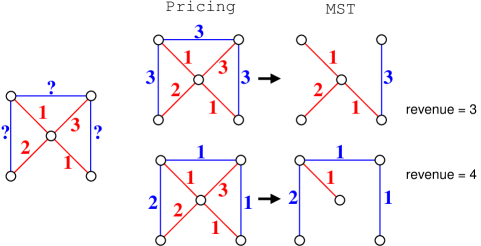
Figure 1: A sample instance of the StackMST problem. The goal is to assign prices to the blue edges to maximize the total price of the blue edges purchased in a minimum spanning tree.

This problem is called the Stackelberg Minimum Spanning Tree Game CDF⁺ (11), and is an example in the growing family of algorithmic game-theoretic problems about combinatorial optimization in graphs GvHvdK⁺ (05); RSM (05); BHK (08); vH (06); BGPW (08); GvLSU (09); BHGV (09); BGLP (10); BCK⁺ (10). More formally, we are given an undirected graph $G$ (possibly with parallel edges, but no loops), whose edge set $E(G)$ is partitioned into a red edge set $R(G)$ and a blue edge set $B(G)$. We are also given a cost function $c:R(G)\to{\mathbb{R}}^{+}$ assigning a positive cost to each red edge. The StackMST problem is to assign a price $p(e)$ to each blue edge $e$, resulting in a weighted graph $(G,c\cup p)$, to maximize the total price of blue edges in a minimum spanning tree. We assume that, if there is more than one minimum spanning tree, we obtain the maximum possible income. (Otherwise, we could decrease the prices slightly and get arbitrarily close to the same income.) Figure 1 shows an example.

This problem is thus a two-player two-level optimization problem, in which the leader (the company) chooses a strategy (a price assignment), taking into account the strategy of the follower (the client), which is determined by a second-level optimization problem (the minimum spanning tree problem). Such a game is known as a Stackelberg game in economics vS (34).

Motivations and scope.

The Stackelberg Minimum Spanning Tree Game is a suitable model for real-life network pricing problems, of the same flavor as those previously used for taxation and freight tariff-setting in the operations research community (see for instance LMS (98); BLMS (00, 01)). It can be used to model pricing in communication or transportation networks, and is easily amenable to meaningful generalizations (see previous works below).

In this contribution, we aim at studying the problem under two natural restrictions. First, we consider the class of planar instances, i.e., in which the input graph is planar. This can model situations in which the input network corresponds to geographic connections. Many important combinatorial optimization problems admit polynomial-time approximation schemes on planar graphs. Among the first such results, Baker’s technique Bak (94) is well known. Since then, many more powerful techniques have been proposed Kle (05, 06); BKMK (07); DHM (07); DHK (09), which ultimately rely on the ability to efficiently solve the problem in graphs of bounded treewidth in polynomial time.

This leads us to the second structural restriction we will tackle. Bounded-treewidth graphs have the property of being “close” to trees, in the sense that they have can be augmented into chordal graphs with a bounded clique number. They also constitute a natural structural restriction, that may be verified in real-life cases, and have proven fundamental in many other combinatorial problems (see for instance the surveys from Bodlaender Bod (06) and Bodlaender and Koster BK (08)).

Optimization algorithms on bounded-treewidth graphs are generally based on dynamic programming, using a textbook technique for well-behaved problems. In particular, it was shown by Courcelle Cou (08) that the problem of checking a graph-theoretic property expressible in monadic second-order logic is fixed-parameter tractable with respect to the treewidth of the graph. However, few if any such dynamic programs have been developed for a bilevel optimization problem such as StackMST, and standard techniques do not seem to apply. We expect our contribution to give a basis for further application of graph decompositions to other bilevel optimization problems.

Previous results.

The complexity and approximability of the StackMST problem has been studied in a previous paper CDF⁺ (11). It was shown that the problem is APX-hard, but can be approximated within a logarithmic factor. Also, constant-factor approximation exist for the special cases in which the given costs are bounded or take a bounded number of distinct values. Finally, an integer programming formulation has an integrality gap corresponding to the best known approximation factors.

Briest et al. BHK (08) generalized the above results to a wider class of pricing problems on graphs. This includes, in particular, pricing problems with many followers and shortest path pricing games. They show that the single-price strategy proposed in CDF⁺ (11) yields logarithmic approximation factors for these games as well. They also tackle a Stackelberg bipartite vertex cover game, which is shown to be solvable in polynomial time.

Recently, Bilò et al. BGLP (10) studied special cases and another generalization of the StackMST problem. In particular, they show that the problem is approximable within a constant factor whenever the set of blue edges of $G$ forms a complete graph, and is solvable in polynomial time if, additionally, there are only two distinct red costs. The generalization involves activation costs for the blue edges, and a leader with a bounded activation budget. They generalize previous results to that case, and give an approximation factor parameterized by the radius of the spanning tree induced by the red edges.

Our results.

In Section 2, we prove that StackMST remains NP-hard when restricted to planar graphs (Theorem 2.1). The reduction is a strengthening from our previous result, and is from the minimum connected vertex cover problem.

In Section 3, we develop the tools required for the design of a polynomial-time dynamic programming algorithm for StackMST in series-parallel graphs. These graphs have treewidth at most 2 and are planar, and they can be alternatively defined in an inductive fashion using two composition operations. We show (Theorem 3.1) that the StackMST problem can be solved in $O(m^{4})$ time on series-parallel graphs with $m$ edges.

Finally, Section 4 deals with graphs of arbitrary treewidth $t$. Our Theorem 4.1 states that the problem can be solved in $2^{O(t^{3})}m+m^{O(t^{2})}$ time on those graphs.

2 Planar Graphs

We consider the StackMST problem on planar graphs. We strengthen the hardness result given in CDF⁺ (11) by showing that the problem remains NP-hard in this special case. The reduction is from the minimum connected vertex cover problem, which is known to be NP-hard, even when restricted to planar graphs of maximum degree 4 (see Garey and Johnson GJ (79)). The minimum connected vertex cover problem consists of finding a minimum-size subset $C$ of the vertices of a graph, such that every edge has at least one endpoint in $C$, and $C$ induces a connected graph.

Theorem 2.1

The StackMST problem is NP-hard, even when restricted to planar graphs.

Proof

Given a planar graph $G=(V,E)$, with $|V|=n$ and $|E|=m$, we construct an instance of StackMST with red costs in $\{1,2\}$. Let $G^{\prime}=(V^{\prime},R\cup B)$ be the graph for this instance, with $(R,B)$ a bipartition of the edge set. We first let $V^{\prime}=V\cup E$. The set of blue edges $B$ is the set $\{ve:e\in E,v\in e\}$. Thus the blue subgraph is the vertex-edge incidence graph of $G$, which is clearly planar. Given a planar embedding of the blue subgraph, we connect all vertices $e\in E$ of $G^{\prime}$ by a tree, all edges of which are red and have cost $1$. The graph can be kept planar by letting those red edges be nonintersecting chords of the faces of the embedding. Finally, we double all blue edges by red edges of cost 2. The whole construction is illustrated in figure 2(a).

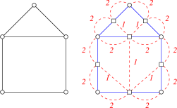
(a) The graphs $G$ and $G^{\prime}$.

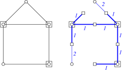
(b) A connected vertex cover in $G$ and the corresponding price function in $G^{\prime}$.

Figure 2: Illustration of the proof of Theorem 2.1.

Let $t$ be a positive integer. We show that the revenue for an optimal price function for $G^{\prime}$ is at least $m+2n-t-1$ if and only if there exists a connected vertex cover of $G$ of size at most $t$.

$(\Leftarrow)$ We first suppose that there exists such a connected vertex cover $C\subseteq V$, and show how to construct a price function yielding the given revenue.

From the set $C$, we can construct a tree made of blue edges that spans all vertices $e\in E$ of $G^{\prime}$. The set of vertices of this tree is $C\cup E$, and its edges are of the form $ue\in E^{\prime}$, with $u\in C$ and $e\in E$ (see figure 2(b)). This tree has $t+m-1$ blue edges, to which we assign price $1$. Now we have to connect the remaining $n-t$ vertices belonging to $V$. Since the only red edges incident to these vertices have cost $2$, we can use $n-t$ blue edges of price $2$ to include these vertices in the minimum spanning tree. The price of the other blue edges is set to $\infty$. The revenue for this price function is exactly $(t+m-1)+2(n-t)=m+2n-t-1$.

$(\Rightarrow)$ Now suppose that we have a price function yielding revenue at least $m+2n-t-1$. We can assume (see CDF⁺ (11)) that all the prices belong to the set $\{1,2,\infty\}$. We also assume that the price function is optimal and minimizes the number of red edges in the resulting spanning tree $T$.

First, we observe that $T$ does not contain any red edge. By contradiction, if $T$ contains a red edge of cost 2, then this edge can be replaced by the parallel blue edge. On the other hand, if $T$ contains a red edge $f$ of cost 1, we consider the cut defined by removing $f$ from $T$. In the face used to define $f$, there exists a blue edge having its endpoints across the cut and does not belong to $T$. So we can use this blue edge, with a price equal to 1, to reconnect the tree.

Now let us consider the blue edges of price $1$ in $T$. We claim that the graph $H$ induced by these edges contains all vertices $e\in E$ of $G^{\prime}$ and is connected.

Clearly, all vertices $e\in E$ of $G^{\prime}$ are incident to a blue edge of price $1$, otherwise it can be reconnected to $T$ with a red edge of cost $1$, and $T$ is not minimum. Thus $E\subseteq V(H)$, where $V(H)$ is the vertex set of $H$. Letting $C:=V(H)\cap V$, we conclude that $C$ is a vertex cover of the original graph $G$.

Now we show that $H$ is connected. Suppose otherwise; then there exist two vertices of $G^{\prime}$ in $E$ that are connected by a red edge of cost $1$, and belonging to two different connected components $H_{1}$ and $H_{2}$ of $H$. Consider the (blue) edge that connects $H_{1}$ and $H_{2}$ in $T$. This edge cannot have price 2 in $T$, since $H_{1}$ and $H_{2}$ are connected by a red edge of cost $1$. Hence the blue edge has price 1 and belongs to $H$. Therefore $H$ is connected and $C$ is a connected vertex cover of $G$.

Finally the remaining vertices $V-C$ of $G^{\prime}$ must be leaves of $T$, since otherwise they belong to a cycle containing a red edge of cost $1$. The total cost of $T$ is therefore $(m+|C|-1)+2(n-|C|)=m+2n-|C|-1$. Since we know this is at least $m+2n-t-1$, we conclude that $|C|\leq t$.

∎

3 Series-Parallel Graphs

We now describe a polynomial-time dynamic programming algorithm for solving the StackMST problem on series-parallel graphs. These graphs are planar and have treewidth at most $2$.

We use the following inductive definition of (connected) series-parallel graphs. Consider a connected graph $G$ with two distinguished vertices $s$ and $t$. The graph $(G,s,t)$ is a series-parallel graph if either $G$ is a single edge $(s,t)$, or $G$ is a series or parallel composition of two series-parallel graphs $(G_{1},s_{1},t_{1})$ and $(G_{2},s_{2},t_{2})$. The series composition of $G_{1}$ and $G_{2}$ is formed by setting $s=s_{1},t=t_{2}$ and identifying $t_{1}=s_{2}$; the parallel composition is formed by identifying $s=s_{1}=s_{2}$ and $t=t_{1}=t_{2}$.

We first give a number of useful lemmas and an outline of the dynamic programming algorithm. This algorithm will use two main rules, corresponding to the series and parallel composition operations. Once the two rules are defined, the description of the algorithm is straightforward.

3.1 Preliminaries

Let us fix an instance of StackMST, that is, a graph $G$ with $E(G)=R(G)\cup B(G)$ endowed with a cost function $c:R(G)\to\mathbb{R}_{+}$. Denote by $c_{1},c_{2},\dots,c_{k}$ the different values taken by $c$, in increasing order. Let also $c_{0}:=0$.

For two distinct vertices $s,t\in V(G)$ of $G$ and a subset $F\subseteq B(G)$ of blue edges, define $\mathcal{P}(G,F,s,t)$ as the set of $st$-paths in the graph $(V(G),R(G)\cup F)$. Let also $\widetilde{\mathcal{P}}(G,F,s,t)$ denote the subset of paths in $\mathcal{P}(G,F,s,t)$ that contain at least one red edge. A lemma of Cardinal et al. CDF⁺ (11) can be restated as follows.

Lemma 1 (CDF⁺ (11))

Suppose that $G$ contains a red spanning tree, and let $F\subseteq B(G)$ be an acyclic subset of blue edges. Then, the maximum revenue achievable by the leader, over solutions where the set of blue edges bought by the follower is exactly $F$, is obtained by setting the price of each edge $st\not\in F$ to $+\infty$, and the price of each edge $st\in F$ to

$$\min\left\{\max_{e\in P\cap R(G)}c(e)\mid P\in\widetilde{\mathcal{P}}(G,F,s,t)\right\}.$$

This lemma states that if we know the set of blue edges that will eventually be bought, the price of a selected blue edge $st$ is given by the minimum, over the paths from $s$ to $t$, of the largest red cost on this path.

Motivated by this result, we introduce some more notations. For a subset $Z\subseteq E(G)$ of edges, we define $\operatorname{mc}(Z)$ as the maximum cost of a red edge in $Z$ if $Z\cap R(G)\neq\varnothing$, as $c_{0}=0$ otherwise. (The two letters $\operatorname{mc}$ stand for “max cost”.) We define $w(G,F,s,t)$ as

$$w(G,F,s,t):=\left\{\begin{array}[]{ll}\min\left\{\operatorname{mc}(P)\mid P\in\mathcal{P}(G,F,s,t)\right\}&\textrm{ if }\mathcal{P}(G,F,s,t)\neq\varnothing;\\ c_{k}&\textrm{ otherwise}.\end{array}\right.$$

Similarly,

$$\widetilde{w}(G,F,s,t):=\left\{\begin{array}[]{ll}\min\left\{\operatorname{mc}(P)\mid P\in\widetilde{\mathcal{P}}(G,F,s,t)\right\}&\textrm{ if }\widetilde{\mathcal{P}}(G,F,s,t)\neq\varnothing;\\ c_{k}&\textrm{ otherwise}.\end{array}\right.$$

Thus, the price assigned to the edge $st\in F$ in Lemma 1 is $\widetilde{w}(G,F,s,t)$. Also, for the purpose of induction, we will consider graphs that do not necessarily contain a red spanning tree; this is why we need to treat the case where $\mathcal{P}(G,F,s,t)$ or $\widetilde{\mathcal{P}}(G,F,s,t)$ is empty in the above definitions.

In what follows, we let $[k]:=\{0,1,\ldots,k\}$. Our dynamic programming solution for series-parallel graphs associates a value to each pair $(H,q)$, where $q\in[k]^{2}$, and $H$ is a graph appearing in the series-parallel decomposition of $G$.

A subset $F\subseteq B(G)$ of blue edges realizes $q=(i,j)\in[k]^{2}$ in $(G,s,t)$ if $F$ is acyclic and $w(G,F,s,t)=c_{i}$. Although this property does not depend on $j$, the formulation will appear to be convenient. Similarly, we say that $q$ is realizable in $(G,s,t)$ if there exists such a subset $F$.

For $j\in[k]$ and distinct vertices $s,t\in V(G)$, let $G^{+}$ denote the graph $G$ with an additional red edge between $s$ and $t$ of cost $c_{j}$. We define

$$\operatorname{OPT}_{(i,j)}(G,s,t):=\max\left.\left\{\sum_{uv\in F}\widetilde{w}(G^{+},F,u,v)\,\right|F\subseteq B(G),F\textrm{ realizes }(i,j)\textrm{ in }(G,s,t)\right\},$$

if such a subset $F$ exists, and set $\operatorname{OPT}_{(i,j)}(G,s,t):=-\infty$ otherwise.

Intuitively, we want to keep track of optimal acyclic subsets of blue edges for every graph $G$ obtained during the construction of a series-parallel graph. The problem is, that the weights of the blue edges in the optimal solution might change as we compose graphs in the series-parallel decomposition. However, the weights of edges depend only on the maximum red costs, or bottlenecks, of the new $st$-paths that will be added to $G$. We can thus prepare $\operatorname{OPT}(G,s,t)$ for every possible set of bottlenecks. These bottlenecks are the values $j$ in what precedes. The value $i$ then corresponds to the new bottleneck that is realized, to be taken into account in future compositions.

Note that by Lemma 1, if $G$ has a red spanning tree, then the maximum revenue achievable by the leader on instance $G$ equals

$$\max_{i\in[k]}\operatorname{OPT}_{(i,k)}(G,s,t).$$

This will be the result returned by the dynamic programming solution.

3.2 Series Compositions

Let $q=(i,j)$, $q_{1}=(i_{1},j_{1})$, and $q_{2}=(i_{2},j_{2})$, with $q,q_{1},q_{2}\in[k]^{2}$. We say that the pair $(q_{1},q_{2})$ is series-compatible with $q$ if

1. $\max\{i_{1},i_{2}\}=i$;

2. $\max\{j,i_{2}\}=j_{1}$, and

3. $\max\{j,i_{1}\}=j_{2}$,

Notice that $(q_{1},q_{2})$ is series-compatible with $q$ if and only if $(q_{2},q_{1})$ is.

This condition allows us to use the following recursion in our dynamic programming algorithm.

Lemma 2

Suppose that $(G,s,t)$ is a series composition of $(G_{1},s_{1},t_{1})$ and $(G_{2},s_{2},t_{2})$, and that $q\in[k]^{2}$ is realizable in $(G,s,t)$. Then

$$\operatorname{OPT}_{q}(G,s,t)=\max\left\{\operatorname{OPT}_{q_{1}}(G_{1},s_{1},t_{1})+\operatorname{OPT}_{q_{2}}(G_{2},s_{2},t_{2})\mid(q_{1},q_{2})\text{\ is\ series-compatible\ with\ }q\right\}.$$

We now prove that the recursion is valid. We need the following lemmas. In what follows, $(G,s,t)$ is a series composition of $(G_{1},s_{1},t_{1})$ and $(G_{2},s_{2},t_{2})$; $q,q_{1},q_{2}\in[k]^{2}$ with $q=(i,j)$, $q_{1}=(i_{1},j_{1})$, and $q_{2}=(i_{2},j_{2})$ are such that $(q_{1},q_{2})$ is series-compatible with $q$; and $F_{\ell}\subseteq B(G_{\ell})$ realizes $q_{\ell}$ in $(G_{\ell},s,t)$, for $\ell=1,2$.

We first observe that $F:=F_{1}\cup F_{2}$ realizes $q$.

Lemma 3

$F$ realizes $q$ in $(G,s,t)$.

Proof

Since $V(G_{1})\cap V(G_{2})=\{t_{1}\}$ ($=\{s_{2}\}$), the set $F$ is clearly acyclic. It remains to show $w(G,F,s,t)=c_{i}$. Every $st$-path in $\mathcal{P}(G,F,s,t)$ is the combination of an $s_{1}t_{1}$-path of $\mathcal{P}(G_{1},F_{1},s_{1},t_{1})$ with an $s_{2}t_{2}$-path of $\mathcal{P}(G_{2},F_{2},s_{2},t_{2})$. It follows

$$w(G,F,s,t)=\max\left\{w(G_{1},F_{1},s_{1},t_{1}),w(G_{2},F_{2},s_{2},t_{2})\right\}=\max\{c_{i_{1}},c_{i_{2}}\}=c_{i},$$

where the last equality is from (S1).

∎

The proof of the next lemma is illustrated on Figure 3. It motivates the definition of series-compatibility.

Lemma 4

Let $G^{+}$ be the graph $G$ augmented with a red edge $st$ of cost $c_{j}$, and $G_{\ell}^{+}$ (for $\ell=1,2$) the graph $G_{\ell}$ augmented with a red edge $s_{\ell}t_{\ell}$ of cost $c_{j_{\ell}}$. Then for $\ell=1,2$ and every edge $uv\in F_{\ell}$,

$$\widetilde{w}(G^{+},F,u,v)=\widetilde{w}(G_{\ell}^{+},F_{\ell},u,v).$$

Proof

We prove the statement for $\ell=1$, the case $\ell=2$ follows by symmetry. Let $uv\in F_{1}$, and let $e=st$ and $e_{1}=s_{1}t_{1}$ be the additional red edges in $G^{+}$ and $G^{+}_{1}$, respectively.

We first show:

Claim

$\widetilde{w}(G^{+},F,u,v)\geq\widetilde{w}(G_{1}^{+},F_{1},u,v)$.

Proof

The claim is true if $\widetilde{\mathcal{P}}(G^{+},F,u,v)=\varnothing$, since then $\widetilde{w}(G^{+},F,u,v)=c_{k}\geq\widetilde{w}(G_{1}^{+},F_{1},u,v)$. Suppose thus $\widetilde{\mathcal{P}}(G^{+},F,u,v)\neq\varnothing$, and let $P\in\widetilde{\mathcal{P}}(G^{+},F,u,v)$. It is enough to show that $\operatorname{mc}(P)\geq\widetilde{w}(G_{1}^{+},F_{1},u,v)$. This clearly holds if $e\notin E(P)$, as $P$ belongs then also to $\widetilde{\mathcal{P}}(G_{1}^{+},F_{1},u,v)$ (recall that $|V(G_{1})\cap V(G_{2})|=1$). Hence, we may assume $e\in E(P)$. It follows $s_{1},t_{1}\in V(P)$.

Let $s_{1}Pt_{1}$ denote the subpath of $P$ comprised between $s_{1}$ and $t_{1}$. Also let $P_{1}$ denote the path of $\widetilde{\mathcal{P}}(G_{1}^{+},F_{1},u,v)$ obtained by replacing the subpath $s_{1}Pt_{1}$ of $P$ with the edge $e_{1}$. Using (S2), we obtain

$$\operatorname{mc}(s_{1}Pt_{1})=\max\{c_{j},\operatorname{mc}(t_{2}Pt_{1})\}\geq\max\{c_{j},c_{i_{2}}\}=c_{j_{1}},$$

implying $\operatorname{mc}(P)\geq\operatorname{mc}(P_{1})\geq\widetilde{w}(G_{1}^{+},F_{1},u,v)$.

∎

Conversely, we prove:

Claim

$\widetilde{w}(G^{+},F,u,v)\leq\widetilde{w}(G_{1}^{+},F_{1},u,v)$.

Proof

Again, this trivially holds if $\widetilde{\mathcal{P}}(G_{1}^{+},F_{1},u,v)$ is empty. Suppose thus $\widetilde{\mathcal{P}}(G_{1}^{+},F_{1},u,v)\neq\varnothing$, and let $P_{1}\in\widetilde{\mathcal{P}}(G_{1}^{+},F_{1},u,v)$. Similarly as before, it is enough to show that $\widetilde{w}(G^{+},F,u,v)\leq\operatorname{mc}(P_{1})$. This is true if $e_{1}\notin E(P_{1})$, since then $P_{1}\in\widetilde{\mathcal{P}}(G^{+},F,u,v)$. Assume thus $e_{1}\in E(P_{1})$.

If $\mathcal{P}(G_{2},F_{2},s_{2},t_{2})=\varnothing$, then $i_{2}=k$ and $\operatorname{mc}(P_{1})\geq c_{j_{1}}=\max\{c_{j},c_{i_{2}}\}=c_{k}\geq\widetilde{w}(G^{+},F,u,v)$ by (S2). We may thus assume that $\mathcal{P}(G_{2},F_{2},s_{2},t_{2})$ contains a path $P_{2}$; we choose $P_{2}$ such that $\operatorname{mc}(P_{2})=c_{i_{2}}$.

Denote by $P$ the path obtained from $P_{1}$ by replacing the edge $e_{1}$ with the combination of edge $e$ and path $P_{2}$. Since $P\in\widetilde{\mathcal{P}}(G^{+},F,u,v)$, (S2) yields

$$\operatorname{mc}(P_{1}) =\max\left\{c_{j_{1}},\operatorname{mc}(P_{1}-e_{1})\right\}$$

$$=\max\left\{c_{j},c_{i_{2}},\operatorname{mc}(P_{1}-e_{1})\right\}$$

$$=\max\left\{c_{j},\operatorname{mc}(P_{2}),\operatorname{mc}(P_{1}-e_{1})\right\}$$

$$=\operatorname{mc}(P)$$

$$\geq\widetilde{w}(G^{+},F,u,v).$$

∎

The lemma follows from Claims 3.2 and 3.2.

∎

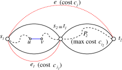
Figure 3: Series composition: illustration of the proof of Lemma 4.

We are now ready to prove the correctness of the recursion step in Lemma 2.

Proof (Proof of Lemma 2)

Let $q$ and $G^{+}$ be defined as before. We first show:

Claim

There exist $q_{1},q_{2}\in[k]^{2}$ such that $(q_{1},q_{2})$ is series-compatible with $q$ and $\operatorname{OPT}_{q}(G,s,t)\leq\operatorname{OPT}_{q_{1}}(G_{1},s,t)+\operatorname{OPT}_{q_{2}}(G_{2},s,t)$.

Proof

Let $F\subseteq B(G)$ be a subset of blue edges realizing $q$ in $(G,s,t)$ such that

$$\operatorname{OPT}_{q}(G,s,t)=\sum_{uv\in F}\widetilde{w}(G^{+},F,u,v).$$

For $\ell=1,2$, let also $F_{\ell}:=F\cap E(G_{\ell})$ and $q_{\ell}:=(i_{\ell},j_{\ell})$, with $i_{\ell}$ the index such that $c_{i_{\ell}}=w(G_{\ell},F_{\ell},s_{\ell},t_{\ell})$, and $j_{\ell}:=\max\{j,i_{\ell+1}\}$ (indices are taken modulo 2). $F_{\ell}$ ($\ell=1,2$) clearly realizes $q_{\ell}$ in $(G_{\ell},s_{\ell},t_{\ell})$. It is also easily verified that $(q_{1},q_{2})$ is series-compatible with $q$. Hence we can apply Lemma 4:

$$\operatorname{OPT}_{q}(G,s,t) =\sum_{uv\in F}\widetilde{w}(G^{+},F,u,v)$$

$$=\sum_{uv\in F_{1}}\widetilde{w}(G^{+}_{1},F_{1},u,v)+\sum_{uv\in F_{2}}\widetilde{w}(G^{+}_{2},F_{2},u,v)$$

$$\leq\operatorname{OPT}_{q_{1}}(G_{1},s_{1},t_{1})+\operatorname{OPT}_{q_{2}}(G_{2},s_{2},t_{2}),$$

as claimed.

∎

We now prove:

Claim

$\operatorname{OPT}_{q}(G,s,t)\geq\operatorname{OPT}_{q_{1}}(G_{1},s_{1},t_{1})+\operatorname{OPT}_{q_{2}}(G_{2},s_{2},t_{2})$ holds for every $q_{1},q_{2}\in[k]^{2}$ such that $(q_{1},q_{2})$ is series-compatible with $q$.

Proof

Suppose that $(q_{1},q_{2})$ is series-compatible with $q$. Let $F_{\ell}\subseteq B(G_{\ell})$ ($\ell=1,2$) be a subset of blue edges of $G_{\ell}$ such that

$$\operatorname{OPT}_{q_{\ell}}(G_{\ell},s_{\ell},t_{\ell})=\sum_{uv\in F_{\ell}}\widetilde{w}(G^{+}_{\ell},F_{\ell},u,v).$$

By Lemma 3, $F:=F_{1}\cup F_{2}$ realizes $q$ in $(G,s,t)$. Using again Lemma 4, we have:

$$\operatorname{OPT}_{q}(G,s,t) \geq\sum_{uv\in F}\widetilde{w}(G^{+},F,u,v)$$

$$=\sum_{uv\in F_{1}}\widetilde{w}(G^{+}_{1},F_{1},u,v)+\sum_{uv\in F_{2}}\widetilde{w}(G^{+}_{2},F_{2},u,v)$$

$$=\operatorname{OPT}_{q_{1}}(G_{1},s_{1},t_{1})+\operatorname{OPT}_{q_{2}}(G_{2},s_{2},t_{2}),$$

and the claim follows.

∎

The lemma follows from Claims 3.2 and 3.2.

∎

3.3 Parallel Compositions

The recursion step for parallel compositions follows a similar scheme. Let $q,q_{1},q_{2}\in[k]^{2}$ with $q=(i,j)$, $q_{1}=(i_{1},j_{1})$, and $q_{2}=(i_{2},j_{2})$. We say that the pair $(q_{1},q_{2})$ is parallel-compatible with $q$ if

1. at least one of $i_{1},i_{2}$ is non-zero;

2. $\min\{i_{1},i_{2}\}=i$;

3. $\min\{j,i_{2}\}=j_{1}$, and

4. $\min\{j,i_{1}\}=j_{2}$,

The recursion step for parallel composition is as follows.

Lemma 5

Suppose that $(G,s,t)$ is a parallel composition of $(G_{1},s,t)$ and $(G_{2},s,t)$, and that $q\in[k]^{2}$ is realizable in $(G,s,t)$. Then

$$\operatorname{OPT}_{q}(G,s,t)=\max\{\operatorname{OPT}_{q_{1}}(G_{1},s,t)+\operatorname{OPT}_{q_{2}}(G_{2},s,t)\mid(q_{1},q_{2})\text{\ is parallel-compatible\ with\ }q\}.$$

In what follows, $(G,s,t)$ is a parallel composition of $(G_{1},s,t)$ and $(G_{2},s,t)$; $(q_{1},q_{2})$ is parallel-compatible with $q$; and $F_{\ell}\subseteq B(G_{\ell})$ realizes $q_{\ell}$ in $(G_{\ell},s,t)$, for $\ell=1,2$. Also, $F:=F_{1}\cup F_{2}$.

Similarly to Lemma 3, the definition of parallel-compatibility implies the following lemma.

Lemma 6

$F$ realizes $q$ in $(G,s,t)$.

Proof

We have to prove that $F$ is acyclic and that $w(G,F,s,t)=c_{i}$.

First, suppose that $(V(G),F)$ contains a cycle $C$. Since $F_{1}$ and $F_{2}$ are both acyclic, $C$ includes the vertices $s$ and $t$, and moreover $E(G_{1})\cap E(C)$, $E(G_{2})\cap E(C)$ are both non-empty. But then, there is an $st$-path in $(V(G),F_{\ell})$ for $\ell=1,2$, implying $i_{1}=i_{2}=0$, which contradicts (P1). Hence, $F$ is acyclic.

Now, since each path of $\mathcal{P}(G,F,s,t)$ is included in either $\mathcal{P}(G_{1},F_{1},s,t)$ or $\mathcal{P}(G_{2},F_{2},s,t)$, it follows $w(G,F,s,t)=\min\{w(G_{1},F_{1},s,t),w(G_{2},F_{2},s,t)\}=\min\{c_{i_{1}},c_{i_{2}}\}$, which equals $c_{i}$ by (P2).

∎

The next lemma is the analogue of Lemma 4 for parallel compositions.

Lemma 7

Let $G^{+}$ be the graph $G$ augmented with a red edge $st$ of cost $c_{j}$, and let $G_{\ell}^{+}$ (for $\ell=1,2$) be the graph $G_{\ell}$ augmented with a red edge $s_{\ell}t_{\ell}$ of cost $c_{j_{\ell}}$. Then for $\ell=1,2$ and every edge $uv\in F_{\ell}$,

$$\widetilde{w}(G^{+},F,u,v)=\widetilde{w}(G_{\ell}^{+},F_{\ell},u,v).$$

Proof

We prove the statement for $\ell=1$, the case $\ell=2$ follows by symmetry. Let $e=st$ and $e_{1}=s_{1}t_{1}$ be the additional red edges in $G^{+}$ and $G^{+}_{1}$, respectively.

Let $uv\in F_{1}$. Observe that $\widetilde{\mathcal{P}}(G^{+},F,u,v)$ is empty if and only if $\widetilde{\mathcal{P}}(G_{1}^{+},F_{1},u,v)$ is. If both are empty, then $\widetilde{w}(G^{+},F,u,v)=\widetilde{w}(G_{1}^{+},F_{1},u,v)=c_{k}$, and the claim holds. Hence, we may assume $\widetilde{\mathcal{P}}(G^{+},F,u,v)\neq\varnothing$ and $\widetilde{\mathcal{P}}(G_{1}^{+},F_{1},u,v)\neq\varnothing$.

We first show:

Claim

$\widetilde{w}(G^{+},F,u,v)\leq\widetilde{w}(G_{1}^{+},F_{1},u,v)$.

Proof

Let $P_{1}\in\widetilde{\mathcal{P}}(G_{1}^{+},F_{1},u,v)$. It is enough to show $\widetilde{w}(G^{+},F,u,v)\leq\operatorname{mc}(P_{1})$. If $e_{1}\notin E(P_{1})$, then $P_{1}\in\widetilde{\mathcal{P}}(G^{+},F,u,v)$, and $\widetilde{w}(G^{+},F,u,v)\leq\operatorname{mc}(P_{1})$ holds by definition. Hence we may assume $e_{1}\in E(P_{1})$.

By (P3), we have $j_{1}=\min\{j,i_{2}\}$. If $j_{1}=j$, then replacing the edge $e_{1}$ of $P_{1}$ by $e$ yields a path $P\in\widetilde{\mathcal{P}}(G^{+},F,u,v)$ with $\operatorname{mc}(P)=\operatorname{mc}(P_{1})$, implying $\widetilde{w}(G^{+},F,u,v)\leq\operatorname{mc}(P_{1})$. Similarly, if $j_{1}=i_{2}<j$, then $i_{2}<k$, implying that $\mathcal{P}(G_{2},F_{2},s,t)$ is not empty. Replacing in $P_{1}$ the edge $e_{1}$ with any path $P_{2}\in\mathcal{P}(G_{2},F_{2},s,t)$ with $\operatorname{mc}(P_{2})=c_{i_{2}}$ gives again a path $P$ with $\operatorname{mc}(P)=\operatorname{mc}(P_{1})$. While the path $P_{2}$ does not necessarily contain a red edge, the path $P$, on the other hand, cannot be completely blue. This is because otherwise $F$ contains the cycle $P\cup\{uv\}$, contradicting the fact that $F$ is acyclic (as follows from Lemma 6). Hence, $P\in\widetilde{\mathcal{P}}(G^{+},F,u,v)$, and $\widetilde{w}(G^{+},F,u,v)\leq\operatorname{mc}(P)=\operatorname{mc}(P_{1})$. Claim 3.3 follows.

∎

Conversely, we prove:

Claim

$\widetilde{w}(G^{+},F,u,v)\geq\widetilde{w}(G_{1}^{+},F_{1},u,v)$.

Proof

Let $P\in\widetilde{\mathcal{P}}(G^{+},F,u,v)$. Again, it is enough to show $\operatorname{mc}(P)\geq\widetilde{w}(G_{1}^{+},F_{1},u,v)$. This clearly holds if $P\in\widetilde{\mathcal{P}}(G^{+}_{1},F_{1},u,v)$. Hence, we may assume $s,t\in V(P)$, and that the subpath $sPt$ of $P$ either belongs to $\mathcal{P}(G_{2},F_{2},s,t)$, or corresponds to the edge $e$ (by $sPt$ we denote the subpath of $P$ that is between vertices $s$ and $t$).

In the first case, $c_{i_{2}}\leq\operatorname{mc}(sPt)$ holds by definition. Moreover, $j_{1}\leq i_{2}$ follows from (P3). Therefore, replacing the subpath $sPt$ of $P$ with the edge $e_{1}$ yields a path $P_{1}\in\widetilde{\mathcal{P}}(G_{1}^{+},F_{1},u,v)$ with $\operatorname{mc}(P_{1})\leq\operatorname{mc}(P)$, implying $\widetilde{w}(G_{1}^{+},F_{1},u,v)\leq\operatorname{mc}(P)$.

Similarly, (P3) implies $j_{1}\leq j$ in the second case. Hence, replacing the edge $e$ of $P$ with $e_{1}$ results in a path $P_{1}\in\widetilde{\mathcal{P}}(G_{1}^{+},F_{1},u,v)$ with $\operatorname{mc}(P_{1})\leq\operatorname{mc}(P)$, showing $\widetilde{w}(G_{1}^{+},F_{1},u,v)\leq\operatorname{mc}(P)$. This completes the proof of Claim 3.3.

∎

Lemma 7 follows from Claims 3.3 and 3.3.

∎

Using the two previous lemmas, the proof of Lemma 5 is the same as that of Lemma 2 for series composition. We omit it.

3.4 The Algorithm

Theorem 3.1

The StackMST problem can be solved in $O(m^{4})$ time on series-parallel graphs.

Proof

A series-parallel decomposition of a connected series-parallel graph can be computed in linear time VTL (82). Given such a decomposition, Lemmas 2 and 5 yield the following algorithm: consider each graph $(H,s,t)$ in the decomposition tree in a bottom-up fashion.

If $H$ is a single edge $st$, we directly compute $\operatorname{OPT}_{q}(H,s,t)$ for every $q\in[k]^{2}$. In particular, if $H$ is a single red edge of cost $c_{h}$, then $\operatorname{OPT}_{(i,j)}(H,s,t)=0$ if $i=h$, and $-\infty$ otherwise. On the other hand, if $H$ is a single blue edge, then $\operatorname{OPT}_{(i,j)}(H,s,t)$ is equal to $c_{j}$ if $i=0$ (corresponding to the case $F=\{st\}$), to $0$ if $i=k$ (corresponding to the case $F=\varnothing$), and to $-\infty$ otherwise.

If $(H,s,t)$ is a series or parallel composition of $(H_{1},s_{1},t_{1})$ and $(H_{2},s_{2},t_{2})$, compute $\operatorname{OPT}_{q}(H,s,t)$ for every $q\in[k]^{2}$ based on the previously computed values for $(H_{1},s_{1},t_{1})$ and $(H_{2},s_{2},t_{2})$, relying on Lemmas 2 and 5.

For every $q=(i,j)\in[k]^{2}$, there are $O(k)$ possible values for either series-compatible or parallel-compatible pairs $(q_{1},q_{2})$. Hence every step costs $O(k)$ times. Since there are $O(k^{2})$ possible values for $q$, and $O(m)$ graphs in the decomposition of $G$, the overall complexity is $O(k^{3}m)=O(m^{4})$.

This results in a polynomial-time algorithm computing the maximum revenue achievable by the leader. Moreover, using Lemmas 3 and 6, it is not difficult to keep track at each step of a witness $F\subseteq B(H)$ for $\operatorname{OPT}_{q}(H,s,t)$, whenever $\operatorname{OPT}_{q}(H,s,t)>-\infty$. This proves the theorem.

∎

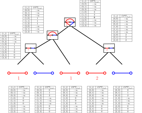
Figure 4: An example of execution of the dynamic programming algorithm for StackMST on series-parallel graphs. The graph is constructed using two series compositions and two parallel compositions. The pairs $(i,j),OPT_{(i,j)}(H,s,t)$ are shown for each intermediate graph $(H,s,t)$ of the decomposition. The value 3 shown in boldface in the top table is the maximum achievable profit.

An example of execution of the algorithm is given in figure 4.

4 Bounded-Treewidth Graphs

In the previous section, we gave a polynomial-time algorithm for solving the StackMST problem on series-parallel graphs, which have treewidth at most $2$. In this section, we extend the algorithm to handle graphs of bounded treewidth, as indicated by the following theorem.

Theorem 4.1

The StackMST problem can be solved in $2^{O(t^{3})}m+m^{O(t^{2})}$ time on graphs of treewidth $t$.

The treewidth of a graph $G$ is usually defined as the minimum width of a tree decomposition of $G$. Since we will not use tree decompositions explicitly, we skip the definition (see for instance Die (05)). Instead we will rely on the fact, first proved by Abrahamson and Fellows AF (93), that every graph of treewidth $t$ is isomorphic to a $t$-boundaried graph, which is defined as a graph with $t$ distinguished vertices (called boundary vertices), each uniquely labeled by a label in $\{1,\dots,t\}$, which can be build recursively using the following operators:

1. The null operator $\varnothing$ creates an $t$-boundaried graph having only $t$ boundary vertices, and they are all isolated.

2. The binary operator $\oplus$ takes the disjoint union of two $t$-boundaried graphs and identify the $i$th boundary vertex of the first graph with the $i$th boundary vertex of the second graph. Thus the edges between two boundary vertices of $G_{1}\oplus G_{2}$ correspond to the union of the edges between these vertices in $G_{1}$ and in $G_{2}$. (Observe that this operation is exactly a parallel-composition if there are only two boundary vertices.)

3. The unary operator $\eta$ introduces a new isolated vertex and makes this the new vertex with label 1 in the boundary. The previous vertex that was labeled 1 is removed from the boundary (but not from the graph).

4. The unary operator $\epsilon$ adds an edge between the vertices labeled 1 and 2 in the boundary.

5. Unary operators that permute the labels of the boundary vertices.

We note that, conversely, every $t$-boundaried graph has treewidth at most $t$ (but not necessarily exactly $t$). The set of boundary vertices of a $t$-boundaried graph $G$ is denoted by $\partial(G)$. Every $t$-boundaried graph on $n$ vertices can be constructed by applying $O(tn)$ compositions according to the above five operators. This construction as well as the boundary vertices can be found in $2^{O(t^{3})}m$ time Bod (96) (note that is linear time is $t$ is a fixed constant).

To summarize, in order to prove Theorem 4.1, it is enough to show that the StackMST problem can be solved in $m^{O(t^{2})}$ time on $t$-boundaried graphs when the above-mentioned construction is also given in input.

4.1 Definitions

Consider an instance $G$ of the StackMST problem with $R(G)$ and $B(G)$ denoting the set of red and blue edges, respectively, and with cost function $c:R(G)\to\mathbb{R}_{+}$ on the set of red edges. As usual, denote by $c_{1},c_{2},\dots,c_{k}$ the different values taken by $c$, in increasing order, and let $c_{0}:=0$.

For two distinct vertices $u,v\in V(G)$ of $G$ and a subset $F\subseteq B(G)$ of blue edges, the sets $\mathcal{P}(G,F,u,v)$ and $\widetilde{\mathcal{P}}(G,F,u,v)$ are defined exactly as in Section 3.1, that is, $\mathcal{P}(G,F,u,v)$ is the set of $uv$-paths in $(V(G),R(G)\cup F)$, while $\widetilde{\mathcal{P}}(G,F,u,v)$ denotes the subset of those paths that contain at least one red edge. The corresponding quantities $w(G,F,u,v)$ and $\widetilde{w}(G,F,u,v)$ are also defined as before, that is, $w(G,F,u,v)$ is the minimum of $\operatorname{mc}(P)$ over every path $P\in\mathcal{P}(G,F,u,v)$, with $w(G,F,u,v):=c_{k}$ if there is no such path, and $\widetilde{w}(G,F,u,v)$ is defined in the same way but with respect to $\widetilde{\mathcal{P}}(G,F,u,v)$.

Now let us further assume the instance $G$ is a $t$-boundaried graph, and let us consider two distinct boundary vertices $a,b\in\partial(G)$. An $ab$-path of $G$ is said to be internal if the only boundary vertices of $G$ it includes are $a$ and $b$. For $F\subseteq B(G)$, the sets $\mathcal{P}_{int}(G,F,a,b)$ and $\widetilde{\mathcal{P}}_{int}(G,F,a,b)$ are defined as $\mathcal{P}(G,F,a,b)$ and $\widetilde{\mathcal{P}}(G,F,a,b)$, respectively, but with the additional requirement that the $ab$-paths under consideration are internal $ab$-paths. The quantities $w_{int}(G,F,a,b)$ and $\widetilde{w}_{int}(G,F,a,b)$ are defined with respect to $\mathcal{P}_{int}(G,F,a,b)$ and $\widetilde{\mathcal{P}}_{int}(G,F,a,b)$, respectively, as expected.

For clarity, in what follows we will use the following convention: the letters $a$ and $b$ will always denote vertices in the boundary of $G$, while $u$ and $v$ will be used for arbitrary (possibly non-boundary) vertices of $G$.

A $k$-graph on the boundary of $G$, or simply $k$-graph when $G$ is clear from the context, is a triple $I=(K,f,g)$ where $K$ is a complete graph with vertex set $\partial(G)$, and $f:E(K)\to[k]$ and $g:E(K)\to[k]$ are two functions assigning weights in $[k]$ to the edges of $K$. (Let us recall that, by our convention, $[k]$ denotes the set $\{0,1,\dots,k\}$.) We say that a subset $F\subseteq B(G)$ of blue edges of $G$ realizes a $k$-graph $I=(K,f,g)$ if $F$ is acyclic, and for every two distinct vertices $a,b\in\partial(G)$ we have $w_{int}(G,F,a,b)=c_{f(ab)}$ (thus there is no condition on $g$). The $k$-graph $I$ is said to be realizable in $G$ if there exists such a subset $F$ of blue edges. Notice that this is a direct extension of the notion of realizability introduced in Section 3.1 for series-parallel graphs. We define $G+I$ as the ($t$-boundaried) graph obtained from $G$ by adding, for every two distinct vertices $a,b\in\partial(G)$, a red edge connecting $a$ and $b$ with cost $c_{g(ab)}$. We let $\operatorname{OPT}_{I}(G)$ be defined as follows:

$$\operatorname{OPT}_{I}(G):=\max\left.\left\{\sum_{uv\in F}\widetilde{w}(G+I,F,u,v)\,\right|F\subseteq B(G),F\textrm{ realizes }I\textrm{ in }G\right\}.$$

In cases where $OPT_{I}(G)$ is undefined (that is, $I$ is not realizable), then we set $OPT_{I}(G)=-\infty$.

With these definitions, the dynamic program that will be used is a straightforward generalization of the series-parallel case: We store for every $t$-boundaried graph $H$ appearing in the construction of our $t$-boundaried input graph $G$ the value $\operatorname{OPT}_{I}(H)$ for every $k$-graph $I$, together with a corresponding optimal acyclic subset $F$ of blue edges (if $\operatorname{OPT}_{I}(H)>-\infty$). The value returned by the dynamic programming solution is then the maximum of $\operatorname{OPT}_{I}(G)$ over all $k$-graphs $I$, and a corresponding acyclic subset of blue edges of $G$ is returned. By Lemma 1, this is the maximum revenue achievable by the leader.

Now we consider the five operators appearing in the definition of $t$-boundaried graphs, and show for each of them how to compute $\operatorname{OPT}_{I}(G)$ from already computed values when $G$ results from the application of the operator.

4.2 The null operator $\varnothing$

We begin with the null operator $\varnothing$ that creates a new graph $G$ with $t$ isolated boundary vertices labeled $1,\ldots,t$. Consider an arbitrary $k$-graph $I=(K,f,g)$ on the boundary of $G$. If $f(ab)<k$ for some edge $ab\in E(K)$, then $I$ is not realizable in $G$, because there is no internal $ab$-path in $G$. Thus we set $OPT_{I}(G):=-\infty$ in this case.

If, on the other hand, $f(e)=k$ for every $e\in E(K)$, then the subset $F=\varnothing$ of blue edges of $G$ realizes $I$, and it is of course the only one since $B(G)=\varnothing$. Hence we let $OPT_{I}(G):=0$ (associated with the set $F=\varnothing$).

4.3 The binary operator $\oplus$

The $\oplus$ operator is very similar to a parallel-composition of series-parallel graphs. Suppose that $G=G_{1}\oplus G_{2}$, and let $I=(K,f,g)$ be an arbitrary $k$-graph on the boundary of $G$. We extend the notion of parallel-compatibility from Section 3.3 as follows: If $I_{1}=(K_{1},f_{1},g_{1})$ and $I_{2}=(K_{2},f_{2},g_{2})$ are two $k$-graphs, then we say that the pair $(I_{1},I_{2})$ is $\oplus$-compatible with $I$ if $I_{i}$ ($i=1,2$) is realizable in $G_{i}$, and moreover the following five conditions are satisfied for every $e\in E(K)$:

1. at least one of $f_{1}(e)$ and $f_{2}(e)$ is non-zero;

2. $f(e)=\min\{f_{1}(e),f_{2}(e)\}$;

3. $g_{1}(e)=\min\{g(e),f_{2}(e)\}$;

4. $g_{2}(e)=\min\{g(e),f_{1}(e)\}$, and

5. for every cycle $C$ in $K$, there exists $i\in\{1,2\}$ such that $f_{i}(e)>0$ for every $e\in E(C)$.

Our goal is to compute $\operatorname{OPT}_{I}(G)$ based on values already computed for $G_{1}$ and $G_{2}$. This is achieved by the following lemma.

Lemma 8

Assume that $G$, $I$, $G_{1}$ and $G_{2}$ are as above, and suppose further that $I$ is realizable in $G$. Then

$$\operatorname{OPT}_{I}(G)=\max\{\operatorname{OPT}_{I_{1}}(G_{1})+\operatorname{OPT}_{I_{2}}(G_{2})\mid(I_{1},I_{2})\text{\ is }\oplus\text{-compatible with }I\}.$$

(Let us remark that, if $I$ is not realizable in $G$, then we trivially have $\operatorname{OPT}_{I}(G)=-\infty$.) The proof of Lemma 8 is a generalization of the proof of Lemma 5 for parallel compositions and consists of a few steps. First we prove the following lemma, which is similar to Lemma 6.

Lemma 9

Suppose that $I_{i}=(K_{i},f_{i},g_{i})$ is a $k$-graph realized in $G_{i}$ by a subset $F_{i}\subseteq B(G_{i})$ of blue edges of $G_{i}$, for $i=1,2$, and assume further that $(I_{1},I_{2})$ is $\oplus$-compatible with $I$. Then $F:=F_{1}\cup F_{2}$ realizes $I$ in $G$.

Proof

We have to prove that $F$ is acyclic and that $w_{int}(G,F,a,b)=c_{f(ab)}$ for every edge $ab\in E(K)$.

First, suppose that $(V(G),F)$ contains a cycle $C$. Since $F_{1}$ and $F_{2}$ are both acyclic, $C$ includes at least two distinct boundary vertices $a$ and $b$, and moreover $E(G_{1})\cap E(C)$, $E(G_{2})\cap E(C)$ are both non-empty. If $a$ and $b$ are the only boundary vertices in $C$ then there is an $ab$-path in $(V(G),F_{1})$ and an $ab$-path in $(V(G),F_{2})$, implying that $f_{1}(ab)=f_{2}(ab)=0$, which contradicts condition (1) from the definition of $\oplus$-compatibility.

If, on the other hand, $C$ contains at least three boundary vertices, choose an orientation of $C$ and an arbitrary vertex $a_{1}\in\partial(G)\cap V(C)$, and enumerate the vertices in $\partial(G)\cap V(C)$ as $a_{1},a_{2},\dots,a_{p}$ according to the order in which they appear when walking on $C$ from $a_{1}$ in the chosen orientation. By condition (5), there is an index $j\in\{1,2\}$ such that $f_{j}(a_{i}a_{i+1})>0$ for every $i\in\{1,\dots,p\}$ (taking indices modulo $p$). We may assume without loss of generality that this is the case for $j=1$.

For every $i\in\{1,\dots,p\}$, the (oriented) path from $a_{i}$ to $a_{i+1}$ in $C$ is a subgraph of $(V(G),F_{1})$ or $(V(G),F_{2})$, since it does not contain other boundary vertices than $a_{i}$ and $a_{i+1}$. This path cannot be a subgraph of $(V(G),F_{1})$ since $f_{1}(a_{i}a_{i+1})>0$, hence it is contained in $(V(G),F_{2})$. However, it follows then that $C$ itself is a subgraph of $(V(G),F_{2})$, which contradicts the fact that $F_{2}$ is acyclic. Therefore, $F$ must be acyclic.

Now, consider two distinct vertices $a,b\in\partial(G)$. Clearly $\mathcal{P}_{int}(G_{1},F_{1},a,b)\cup\mathcal{P}_{int}(G_{2},F_{2},a,b)\subseteq\mathcal{P}_{int}(G,F,a,b)$. By definition, each path $P\in\mathcal{P}_{int}(G,F,a,b)$ has no other boundary vertices than $a$ and $b$, hence $P$ is included in either $\mathcal{P}_{int}(G_{1},F_{1},a,b)$ or $\mathcal{P}_{int}(G_{2},F_{2},a,b)$. It follows that $\mathcal{P}_{int}(G,F,a,b)=\mathcal{P}_{int}(G_{1},F_{1},a,b)\cup\mathcal{P}_{int}(G_{2},F_{2},a,b)$. This in turn implies $w_{int}(G,F,a,b)=\min\{w_{int}(G_{1},F_{1},a,b),w_{int}(G_{2},F_{2},a,b)\}=\min\{c_{f_{1}(ab)},c_{f_{2}(ab)}\}$, which is equal to $c_{f(ab)}$ by condition (2).

∎

The next lemma is the analogue of Lemma 7 from Section 3.3.

Lemma 10

Let $I_{1}=(K_{1},f_{1},g_{1})$, $I_{2}=(K_{2},f_{2},g_{2})$, $F_{1}$, $F_{2}$, and $F$ be as in Lemma 9. Then, for $i=1,2$, and every edge $uv\in F_{i}$, we have

$$\widetilde{w}(G+I,F,u,v)=\widetilde{w}(G_{i}+I_{i},F_{i},u,v).$$

Proof

We prove the statement for $i=1$, the case $i=2$ follows by symmetry.

For every two distinct vertices $a,b\in\partial(G)$, let $e^{ab}$ and $e_{1}^{ab}$ be the additional red edges in $G+I$ and $G+I_{1}$, respectively, between the boundary vertices $a$ and $b$.

Let $uv\in F_{1}$. We first show:

Claim

$\widetilde{w}(G+I,F,u,v)\leq\widetilde{w}(G+I_{1},F_{1},u,v)$.

Proof

If $\widetilde{\mathcal{P}}(G+I_{1},F_{1},u,v)$ is empty then trivially $\widetilde{w}(G+I,F,u,v)\leq c_{k}=\widetilde{w}(G+I_{1},F_{1},u,v)$, thus we may assume $\widetilde{\mathcal{P}}(G+I_{1},F_{1},u,v)\neq\varnothing$.

Let $P_{1}$ be a path in $\widetilde{\mathcal{P}}(G+I_{1},F_{1},u,v)$ with $\operatorname{mc}(P_{1})=\widetilde{w}(G+I_{1},F_{1},u,v)$ and minimizing its length. We will show the existence of a path $P$ in in $\widetilde{\mathcal{P}}(G+I,F,u,v)$ with $\operatorname{mc}(P)\leq\operatorname{mc}(P_{1})$. Since $\widetilde{w}(G+I,F,u,v)\leq\operatorname{mc}(P)$, this will imply the claim.

If $P_{1}$ includes at most one boundary vertex, then $P_{1}\in\widetilde{\mathcal{P}}(G+I,F,u,v)$ and we are done. Hence we may assume that $P_{1}$ includes at least two boundary vertices. Enumerate the boundary vertices that are included in $P_{1}$ as $a_{1},\dots,a_{p}$, in the order in which they appear when going from $u$ to $v$. Let $X$ be the set of indices $i\in\{1,\dots,p-1\}$ such that the subpath $a_{i}P_{1}a_{i+1}$ of $P_{1}$ consists of the edge $e_{1}^{a_{i}a_{i+1}}$. The latter edges are exactly the edges of $P_{1}$ that do no exist in $G+I$. (Note that there could be none, that is, $X$ could be empty.)

For every $i\in X$, we have by condition (3) from the definition of $\oplus$-compatibility that $g_{1}(a_{i}a_{i+1})$ is equal to the minimum of $g(a_{i}a_{i+1})$ and $f_{2}(a_{i}a_{i+1})$. We define an internal $a_{i}a_{i+1}$-path $Q_{i}$ as follows: If $g_{1}(a_{i}a_{i+1})=g(a_{i}a_{i+1})$, then $Q_{i}$ consists simply of the edge $e^{a_{i}a_{i+1}}$. Otherwise, we let $Q_{i}$ be a path in $\mathcal{P}_{int}(G_{2},F_{2},a_{i},a_{i+1})$ with $\operatorname{mc}(Q_{i})=f_{2}(a_{i}a_{i+1})=g_{1}(a_{i}a_{i+1})$. (Observe that such a path exists since $F_{2}$ realizes $I_{2}$ in $G_{2}$.) In both cases, $Q_{i}$ is a path which is a subgraph of $G+I$.

We claim that, for every $i,j\in X$ with $i<j$, the path $Q_{i}$ is internally disjoint from $Q_{j}$ (that is, the only vertex they may have in common is $a_{i+1}$ provided $j=i+1$). Arguing by contradiction, assume otherwise. Then the union of $Q_{i}$ and $Q_{j}$ contains an internal $a_{i}a_{j+1}$-path $R$, and this path satisfies $\operatorname{mc}(R)\leq\max\{\operatorname{mc}(Q_{i}),\operatorname{mc}(Q_{j})\}=\max\{g_{1}(a_{i}a_{i+1}),g_{1}(a_{j}a_{j+1})\}\leq\operatorname{mc}(P_{1})$. But then it follows from condition (3) that $g_{1}(a_{i}a_{j+1})\leq\operatorname{mc}(R)\leq\operatorname{mc}(P_{1})$. Thus, replacing the $a_{i}P_{1}a_{j+1}$ subpath of $P_{1}$ with the edge $e_{1}^{a_{i}a_{j+1}}$ gives a path $P^{\prime}_{1}$ in $\widetilde{\mathcal{P}}(G+I_{1},F_{1},u,v)$ with $\operatorname{mc}(P^{\prime}_{1})\leq\operatorname{mc}(P_{1})=\widetilde{w}(G+I_{1},F_{1},u,v)$ (and hence with $\operatorname{mc}(P^{\prime}_{1})=\widetilde{w}(G+I_{1},F_{1},u,v)$), which is shorter than $P_{1}$, a contradiction.

For each $i\in X$, the path $Q_{i}$ has no other vertex in common with $P_{1}$ than its two endpoints (since $Q_{i}$ is an internal $a_{i}a_{i+1}$-path from $G_{2}$). Relying on the fact that the $Q_{i}$’s are pairwise internally disjoint, we let $P$ be the path obtained from $P_{1}$ by replacing, for every $i\in X$, the edge $e_{1}^{a_{i}a_{i+1}}$ with the path $Q_{i}$. The path $P$ must contain at least one red edge, because otherwise $P+uv$ would be a cycle in $(V(G),F)$, contradicting Lemma 9. Thus $P$ is in $\widetilde{\mathcal{P}}(G+I,F,u,v)$. Moreover, by our choice of the $Q_{i}$’s, we have $\operatorname{mc}(P)\leq\operatorname{mc}(P_{1})$, as desired.

∎

Conversely, we prove:

Claim

$\widetilde{w}(G+I,F,u,v)\geq\widetilde{w}(G+I_{1},F_{1},u,v)$.

Proof

If $\widetilde{\mathcal{P}}(G+I,F,u,v)$ is empty then $\widetilde{w}(G+I,F,u,v)=c_{k}\geq\widetilde{w}(G+I_{1},F_{1},u,v)$, thus we may suppose that $\widetilde{\mathcal{P}}(G+I,F,u,v)$ is not empty.

We have to show that $\operatorname{mc}(P)\geq\widetilde{w}(G+I_{1},F_{1},u,v)$ for every $P\in\widetilde{\mathcal{P}}(G+I,F,u,v)$. Consider such a path $P$. If $P$ includes at most one boundary vertex, then $P\in\widetilde{\mathcal{P}}(G+I,F,u,v)$ and we are done. So assume $P$ contains at least two boundary vertices, and enumerate them as $a_{1},\dots,a_{p}$ as in the proof of the previous claim.

For every $i\in\{1,\dots,p-1\}$, the subpath $Q_{i}:=a_{i}Pa_{i+1}$ of $P$ is either in $\mathcal{P}_{int}(G_{1},F_{1},a_{i},a_{i+1})$, or in $\mathcal{P}_{int}(G_{2},F_{2},a_{i},a_{i+1})$, or consists of the edge $e^{a_{i}a_{i+1}}$. Observe that, in the second case, we have $g_{1}(a_{i}a_{i+1})\leq f_{2}(a_{i}a_{i+1})\leq\operatorname{mc}(Q_{i})$ by condition (3), and in the last case $g_{1}(a_{i}a_{i+1})\leq g(a_{i}a_{i+1})=\operatorname{mc}(Q_{i})$ by the same condition. Hence, if for every $i\in\{1,\dots,p-1\}$ such that $Q_{i}\notin\mathcal{P}_{int}(G_{1},F_{1},a_{i},a_{i+1})$, we replace the subpath $Q_{i}$ of $P$ with the edge $e^{a_{i}a_{i+1}}$, we obtain a path $P_{1}$ which is in $\widetilde{\mathcal{P}}(G+I_{1},F_{1},u,v)$ and which satisfies $\operatorname{mc}(P_{1})\leq\operatorname{mc}(P)$. Since $\widetilde{w}(G+I_{1},F_{1},u,v)\leq\operatorname{mc}(P_{1})$, this completes the proof.

∎

Lemma 10 follows from Claims 4.3 and 4.3.

∎

We may now turn to the proof of Lemma 8.

Proof (Proof of Lemma 8)

We first show:

Claim

There exist $k$-graphs $I_{1}$ and $I_{2}$ such that $(I_{1},I_{2})$ is $\oplus$-compatible with $I$ and $\operatorname{OPT}_{I}(G)\leq\operatorname{OPT}_{I_{1}}(G_{1})+\operatorname{OPT}_{I_{2}}(G_{2})$.

Proof

Let $F\subseteq B(G)$ be a subset of blue edges realizing $I$ in $G$ such that

$$OPT_{I}(G)=\sum_{uv\in F}\widetilde{w}(G+I,F,u,v).$$

For $i=1,2$, let $F_{i}:=F\cap E(G_{i})$, and let $I_{i}=(K_{i},f_{i},g_{i})$ be the $k$-graph obtained by letting, for every $ab\in E(K)$, $f_{i}(ab)$ be the index $j\in[k]$ such that $c_{j}=w_{int}(G_{i},F_{i},a,b)$, and $g_{i}(ab):=\min\{g(ab),f_{i+1}(ab)\}$ (indices are taken modulo 2). Observe that $F_{i}$ realizes $I_{i}$ in $G_{i}$, for $i=1,2$.

Let us show that $(I_{1},I_{2})$ is $\oplus$-compatible with $I$. Condition (1) from the definition of $\oplus$-compatibility is satisfied because otherwise the graph $(V(G),F)$ would have a cycle. It should be clear from the definitions of $I_{1}$ and $I_{2}$ that conditions (2), (3) and (4) are also satisfied. Hence, it remains to check condition (5). Arguing by contradiction, let us assume it is not satisfied, that is, that there exists a cycle in $K$ containing two edges $e$ and $e^{\prime}$ such that $f_{1}(e)=0$ and $f_{2}(e^{\prime})=0$. Such a cycle is said to be bad.

Let $C$ be a shortest bad cycle in $K$. Consider an arbitrary orientation of $C$ and enumerate the vertices of $C$ as $a_{1},a_{2},\dots,a_{p}$, in order. By condition (1), for every $i\in\{1,\dots,p\}$ there is a unique index $j\in\{1,2\}$ such that $f_{j}(a_{i}a_{i+1})=0$ (indices are taken modulo $p$); let $\varphi(i)$ denote this index.

Let $Q_{i}$ be the (unique) $a_{i}a_{i+1}$-path in $(V(G_{\varphi(i)}),F_{\varphi(i)})$, for every $i\in\{1,\dots,p\}$. Note that $Q_{i}$ is necessarily an internal $a_{i}a_{i+1}$-path, that is, $Q_{i}$ does not contain any other boundary vertex than $a_{i}$ and $a_{i+1}$. We claim that the $Q_{i}$’s are pairwise internally disjoint. Assume this is not the case, that is, that $Q_{i}$ and $Q_{j}$ share an internal vertex $v$ for some $i,j\in\{1,\dots,p\}$ with $i<j$. Since $v$ is not a boundary vertex, we must have $\varphi(i)=\varphi(j)$. For simplicity, assume without loss of generality that $\varphi(i)=1$. For every $a\in\{a_{i},a_{i+1}\}$ and $b\in\{a_{j},a_{j+1}\}$ with $a\neq b$, there is an internal $ab$-path in the union of $Q_{i}$ and $Q_{j}$, implying $f_{1}(ab)=0$. If $|C|\geq 4$ then $a$ and $b$ can be chosen such that $ab$ is not an edge of $C$. Then the chord $ab$ splits $C$ into two cycles, at least one of which is bad. However, this implies that there is a bad cycle in $K$ that is shorter than $C$, a contradiction. If $|C|=3$, then it follows that $f_{1}(a_{1}a_{2})=f_{1}(a_{2}a_{3})=f_{1}(a_{3}a_{1})=0$. But we also have $f_{2}(a_{i}a_{i+1})=0$ for some $i\in\{1,2,3\}$ since $C$ is bad, which contradicts condition (1). Since in both cases we reach a contradiction, we deduce that the $Q_{i}$’s must be pairwise internally disjoint.

Let $C^{\prime}$ be obtained from the cycle $C$ by replacing each edge $a_{i}a_{i+1}$ ($i\in\{1,\dots,p\}$) with the path $Q_{i}$. Then $C^{\prime}$ is a cycle, since $Q_{i}$ and $Q_{j}$ are internally disjoint for every $i<j$, and is a subgraph of $(V(G),F)$, contradicting the fact that $F$ is acyclic. Therefore, there cannot be any bad cycle in $K$, and condition (5) holds.

Now that we know that $(I_{1},I_{2})$ is $\oplus$-compatible with $I$, we may apply Lemma 10:

$$OPT_{I}(G) =\sum_{uv\in F}\widetilde{w}(G+I,F,u,v)$$

$$=\sum_{uv\in F_{1}}\widetilde{w}(G+I_{1},F_{1},u,v)+\sum_{uv\in F_{2}}\widetilde{w}(G+I_{2},F_{2},u,v)$$

$$\leq OPT_{I_{1}}(G_{1})+OPT_{I_{2}}(G_{2}).$$

∎

Next we prove:

Claim

$OPT_{I}(G)\geq OPT_{I_{1}}(G_{1})+OPT_{I_{2}}(G_{2})$ holds for every $I_{1},I_{2}$ such that $(I_{1},I_{2})$ is $\oplus$-compatible with $I$.

Proof

Suppose that $(I_{1},I_{2})$ is $\oplus$-compatible with $I$. Let $F_{i}\subseteq B(G_{i})$ ($i=1,2$) be a subset of blue edges of $G_{i}$ realizing $I_{i}$ such that

$$OPT_{I_{i}}(G_{i})=\sum_{uv\in F_{i}}\widetilde{w}(G+I_{i},F_{i},u,v).$$

By Lemma 9, $F:=F_{1}\cup F_{2}$ realizes $I$ in $G$. By Lemma 10, we have:

$$OPT_{I}(G) \geq\sum_{uv\in F}\widetilde{w}(G+I,F,u,v)$$

$$=\sum_{uv\in F_{1}}\widetilde{w}(G+I_{1},F_{1},u,v)+\sum_{uv\in F_{2}}\widetilde{w}(G+I_{2},F_{2},u,v)$$

$$=OPT_{I_{1}}(G_{1})+OPT_{I_{2}}(G_{2}).$$

∎

Lemma 8 follows from Claims 4.3 and 4.3.

∎

4.4 The unary operator $\eta$

Suppose that $G=\eta(G^{\prime})$, that is, that $G$ is obtained from $G^{\prime}$ by adding a new isolated boundary vertex $\tilde{b}$ and labeling it $1$. Thus the vertex $\tilde{a}$ with label $1$ in the boundary of $G^{\prime}$ is no longer a boundary vertex in $G$.

The graphs $G$ and $G^{\prime}$ have exactly the same set of edges. However, an $ab$-path between two distinct boundary vertices $a,b\in\partial(G)\cap\partial(G^{\prime})$ that goes through $\tilde{a}$ is not an internal path in $G^{\prime}$, but could be in $G$ (if the path does not contain any other boundary vertex). This leads us to the following definition. Let $I=(K,f,g)$ be an arbitrary $k$-graph on the boundary of $G$. Then a $k$-graph $I^{\prime}=(K^{\prime},f^{\prime},g^{\prime})$ on the boundary of $G^{\prime}$ is $\eta$-compatible with $I$ if $I^{\prime}$ is realizable in $G^{\prime}$ and, for every two distinct vertices $a,b\in\partial(G)\cap\partial(G^{\prime})$, the following four conditions hold:

1. $f(ab)=\min\big{\{}f^{\prime}(ab),\max\{f^{\prime}(a\tilde{a}),f^{\prime}(\tilde{a}b)\}\big{\}}$;

2. $g^{\prime}(ab)=\min\big{\{}g(ab),\max\{g(a\tilde{b}),g(\tilde{b}b)\}\big{\}}$;

3. $f(a\tilde{b})=k$, and

4. $g^{\prime}(a\tilde{a})=k$.

Lemma 11

Assume that $G$, $I$, and $G^{\prime}$ are as above, and suppose further that $I$ is realizable in $G$. Then

$$\operatorname{OPT}_{I}(G)=\max\{\operatorname{OPT}_{I^{\prime}}(G)\mid I^{\prime}\text{\ is }\eta\text{-compatible with }I\}.$$

(Again, if $I$ is not realizable in $G$, then trivially $\operatorname{OPT}_{I}(G)=-\infty$.) The proof of Lemma 11 is split into a few lemmas, as in the previous section. We begin with the following lemma.

Lemma 12

Suppose that $F^{\prime}\subseteq B(G^{\prime})$ realizes a $k$-graph $I^{\prime}=(K^{\prime},f^{\prime},g^{\prime})$ in $G^{\prime}$ which is $\eta$-compatible with $I$. Then $F:=F^{\prime}$ realizes $I$ in $G$.

Proof

Since $F^{\prime}$ realizes $I^{\prime}$ in $G^{\prime}$, the set $F=F^{\prime}$ is acyclic, we are left with proving that $w_{int}(G,F,a,b)=c_{f(ab)}$ for every edge $ab\in E(K)$. Let thus $ab$ be an arbitrary edge in $E(K)$.

First suppose that $a$ or $b$ is equal to $\tilde{b}$, say without loss of generality $b=\tilde{b}$. Since $b$ is an isolated vertex of $G$, we have $\mathcal{P}_{int}(G,F,a,b)=\varnothing$, and thus $w_{int}(G,F,a,b)=c_{k}$. We also have $f(ab)=k$ by condition (3) from the definition of $\eta$-compatibility; hence $w_{int}(G,F,a,b)=c_{f(ab)}$ as desired.

Next suppose that $a,b\neq\tilde{b}$. For every path $P\in\mathcal{P}_{int}(G,F,a,b)$, either $P$ includes the vertex $\tilde{a}$ or not. If $\tilde{a}\not\in V(P)$, then $P$ is also an internal $ab$-path in $G^{\prime}$. If $\tilde{a}\in V(P)$, then $P$ is not internal in $G^{\prime}$ but $P$ is the concatenation of an internal $a\tilde{a}$-path $P_{1}$ in $G^{\prime}$ with an internal $\tilde{a}b$-path $P_{2}$ in $G^{\prime}$, and thus $\operatorname{mc}(P)=\max\{\operatorname{mc}(P_{1}),\operatorname{mc}(P_{2})\}$. It follows that

$$w_{int}(G,F,a,b)\geq\min\big{\{}w_{int}(G^{\prime},F,a,b),\max\{w_{int}(G^{\prime},F,a,\tilde{a}),w_{int}(G^{\prime},F,\tilde{a},b)\}\big{\}}.$$

Let us show that the reverse inequality also holds. This is easy to see if $w_{int}(G^{\prime},F,a,b)\leq\max\{w_{int}(G^{\prime},F,a,\tilde{a}),w_{int}(G^{\prime},F,\tilde{a},b)\}\big{\}}$, since every path in $\mathcal{P}_{int}(G^{\prime},F,a,b)$ is included in $\mathcal{P}_{int}(G,F,a,b)$, implying $w_{int}(G,F,a,b)\leq w_{int}(G^{\prime},F,a,b)$.

Let us thus assume $w_{int}(G^{\prime},F,a,b)>\max\{w_{int}(G^{\prime},F,a,\tilde{a}),w_{int}(G^{\prime},F,\tilde{a},b)\}\big{\}}$, and let $P_{1}\in\mathcal{P}_{int}(G^{\prime},F,a,\tilde{a})$ and $P_{2}\in\mathcal{P}_{int}(G^{\prime},F,\tilde{a},b)$ be such that $\operatorname{mc}(P_{1})=w_{int}(G^{\prime},F,a,\tilde{a})$ and $\operatorname{mc}(P_{2})=w_{int}(G^{\prime},F,\tilde{a},b)$. Then $P_{1}$ and $P_{2}$ cannot have another vertex in common than $\tilde{a}$, because otherwise their union would contain an $ab$-path $P$ avoiding $\tilde{a}$, which is thus in $\mathcal{P}_{int}(G^{\prime},F,a,b)$. This in turn implies $w_{int}(G^{\prime},F,a,b)\leq\operatorname{mc}(P)\leq\max\{\operatorname{mc}(P_{1}),\operatorname{mc}(P_{2})\}=\max\{w_{int}(G^{\prime},F,a,\tilde{a}),w_{int}(G^{\prime},F,\tilde{a},b)\}\big{\}}$, which contradicts our hypothesis. Hence, $V(P_{1})\cap V(P_{2})=\{\tilde{a}\}$, and the concatenation of $P_{1}$ and $P_{2}$ gives an $ab$-path $P$ which is internal in $G$ (but not in $G^{\prime}$), and which is thus included in $\mathcal{P}_{int}(G,F,a,b)$. This implies $w_{int}(G,F,a,b)\leq\operatorname{mc}(P)=\max\{\operatorname{mc}(P_{1}),\operatorname{mc}(P_{2})\}=\max\{w_{int}(G^{\prime},F,a,\tilde{a}),w_{int}(G^{\prime},F,\tilde{a},b)\}$, as desired.

Therefore,

$$w_{int}(G,F,a,b) =\min\big{\{}w_{int}(G^{\prime},F,a,b),\max\{w_{int}(G^{\prime},F,a,\tilde{a}),w_{int}(G^{\prime},F,\tilde{a},b)\}\big{\}}$$

$$=\min\big{\{}c_{f^{\prime}(ab)},\max\{c_{f^{\prime}(a\tilde{a})},c_{f^{\prime}(\tilde{a}b)}\}\big{\}},$$

which is equal to $c_{f(ab)}$ by condition (1).

∎

Lemma 13

Let $I^{\prime}=(K^{\prime},f^{\prime},g^{\prime})$ and $F^{\prime}$ be as in Lemma 12, and let $F:=F^{\prime}$. Then, for every edge $uv\in F$,

$$\widetilde{w}(G+I,F,u,v)=\widetilde{w}(G^{\prime}+I^{\prime},F,u,v).$$

Proof

For every $ab\in E(K)$, let $e^{ab}$ be the extra red edge in $G+I$ between the boundary vertices $a$ and $b$. Similarly, for every $ab\in E(K^{\prime})$, let $e^{\prime ab}$ be the extra red edge in $G^{\prime}+I^{\prime}$ between the boundary vertices $a$ and $b$.

Let $uv\in F$. The proof consists of three claims.

Claim

If $\widetilde{\mathcal{P}}(G+I,F,u,v)=\varnothing$ or $\widetilde{\mathcal{P}}(G^{\prime}+I^{\prime},F,u,v)=\varnothing$ then $\widetilde{w}(G+I,F,u,v)=\widetilde{w}(G^{\prime}+I^{\prime},F,u,v)=c_{k}$.

Proof

First suppose that $\widetilde{\mathcal{P}}(G+I,F,u,v)=\varnothing$. Then $\widetilde{w}(G+I,F,u,v)=c_{k}$ by definition. If $\widetilde{\mathcal{P}}(G^{\prime}+I^{\prime},F,u,v)=\varnothing$ as well then $\widetilde{w}(G+I,F,u,v)=\widetilde{w}(G^{\prime}+I^{\prime},F,u,v)=c_{k}$, and we are done. Let us thus assume that $\widetilde{\mathcal{P}}(G^{\prime}+I^{\prime},F,u,v)$ is not empty. Every path $P\in\widetilde{\mathcal{P}}(G^{\prime}+I^{\prime},F,u,v)$ contains an extra red edge of the form $e^{{}^{\prime}ab}$ with $a$ or $b$ being equal to $\tilde{a}$, since $\widetilde{\mathcal{P}}(G+I,F,u,v)=\varnothing$. The cost of this extra edge is $c_{g^{\prime}(ab)}$, which is equal to $c_{k}$ by condition (4). It follows that $\operatorname{mc}(P)=c_{k}$, and hence $\widetilde{w}(G^{\prime}+I^{\prime},F,u,v)=c_{k}$, as desired.

Now assume that $\widetilde{\mathcal{P}}(G^{\prime}+I^{\prime},F,u,v)=\varnothing$. We show that this implies $\widetilde{\mathcal{P}}(G+I,F,u,v)=\varnothing$ as well, which reduces this case to the case treated above. Arguing by contradiction, suppose that $\widetilde{\mathcal{P}}(G+I,F,u,v)\neq\varnothing$, and let $P\in\widetilde{\mathcal{P}}(G+I,F,u,v)$. Since $\widetilde{\mathcal{P}}(G^{\prime}+I^{\prime},F,u,v)=\varnothing$, the path $P$ must contain the vertex $\tilde{b}$. The two edges of $P$ incident to $\tilde{b}$ are extra red edges of the form $e^{a\tilde{b}}$ and $e^{b\tilde{b}}$, respectively, with $a,b\in\partial(G)\cap\partial(G^{\prime})$ and $a\neq b$. However, replacing the subpath of $P$ consisting of these two edges with the edge $e^{ab}$ gives a path in $\widetilde{\mathcal{P}}(G+I,F,u,v)$ avoiding $\tilde{b}$, implying that $\widetilde{\mathcal{P}}(G^{\prime}+I^{\prime},F,u,v)$ is not empty, a contradiction. The claim follows.

∎

Claim

If $\widetilde{\mathcal{P}}(G+I,F,u,v)\neq\varnothing$ and $\widetilde{\mathcal{P}}(G^{\prime}+I^{\prime},F,u,v)\neq\varnothing$ then $\widetilde{w}(G+I,F,u,v)\leq\widetilde{w}(G^{\prime}+I^{\prime},F,u,v)$.

Proof

We have to show that $\widetilde{w}(G+I,F,u,v)\leq\operatorname{mc}(P^{\prime})$ for every path $P^{\prime}\in\widetilde{\mathcal{P}}(G^{\prime}+I^{\prime},F,u,v)$. Consider such a path $P^{\prime}$. If $P^{\prime}$ contains no extra red edge (that is, a red edge of the form $e^{\prime ab}$ with $a,b\in\partial(G^{\prime})$), then $P^{\prime}\in\widetilde{\mathcal{P}}(G+I,F,u,v)$, and $\widetilde{w}(G+I,F,u,v)\leq\operatorname{mc}(P^{\prime})$ holds. Thus we may assume that $P^{\prime}$ contains at least one such edge.

If $P^{\prime}$ includes an edge of the form $e^{\prime ab}$ with $a$ or $b$ being equal to $\tilde{a}$, then this edge has cost $c_{g^{\prime}(ab)}=c_{k}$ by condition (4), implying $\operatorname{mc}(P^{\prime})=c_{k}$, and thus we have $\widetilde{w}(G+I,F,u,v)\leq c_{k}=\operatorname{mc}(P^{\prime})$. Hence we may assume that $P^{\prime}$ has no such edge.

Let $H$ be the subgraph of $G+I$ obtained from $P^{\prime}$ as follows: for each each extra red edge $e^{\prime ab}$ included in $P^{\prime}$, replace $e^{\prime ab}$ with $e^{ab}$ if $g^{\prime}(ab)=g(ab)$, with the path consisting of the two edges $e^{a\tilde{b}}$, $e^{\tilde{b}b}$ otherwise. Note that $H$ is connected but is not necessarily a path, since the vertex $\tilde{b}$ could have degree more than $2$ in $H$. On the other hand, we have $\operatorname{mc}(H)=\operatorname{mc}(P^{\prime})$ by condition (2). Also, note that every $uv$-path in $H$ contains at least one red edge (since the edges of $H$ not in $P^{\prime}$ are all red). Let $P$ be such a path. Then $\operatorname{mc}(P)\leq\operatorname{mc}(H)=\operatorname{mc}(P^{\prime})$. Since $P$ is in $\widetilde{\mathcal{P}}(G+I,F,u,v)$, it follows that $\widetilde{w}(G+I,F,u,v)\leq\operatorname{mc}(P)\leq\operatorname{mc}(P^{\prime})$, as desired.

∎

Claim

If $\widetilde{\mathcal{P}}(G+I,F,u,v)\neq\varnothing$ and $\widetilde{\mathcal{P}}(G^{\prime}+I^{\prime},F,u,v)\neq\varnothing$ then $\widetilde{w}(G+I,F,u,v)\geq\widetilde{w}(G^{\prime}+I^{\prime},F,u,v)$.

Proof

We have to show that $\widetilde{w}(G^{\prime}+I^{\prime},F,u,v)\leq\operatorname{mc}(P)$ for every path $P\in\widetilde{\mathcal{P}}(G+I,F,u,v)$. Consider such a path $P$. We proceed similarly as in the proof of the previous claim.

If $P$ contains no extra red edge of $G+I$ then $P\in\widetilde{\mathcal{P}}(G^{\prime}+I^{\prime},F,u,v)$, and $\widetilde{w}(G^{\prime}+I^{\prime},F,u,v)\leq\operatorname{mc}(P)$ holds. Thus we may assume that $P$ contains at least one such edge.

Let $P^{\prime}$ be the path obtained from $P$ as follows: First, for each extra red edge $e^{ab}$ in $P$ with $a,b\neq\tilde{b}$, replace $e^{ab}$ with $e^{\prime ab}$. Now, if $P$ includes the vertex $\tilde{b}$, then it has two extra red edges of the form $e^{a\tilde{b}}$ and $e^{b\tilde{b}}$, respectively, with $a,b\in\partial(G)\cap\partial(G^{\prime})$ and $a\neq b$. Replace then the subpath of $P$ consisting of these two edges with the edge $e^{ab}$. The resulting path $P^{\prime}$ is in $\widetilde{\mathcal{P}}(G^{\prime}+I^{\prime},F,u,v)$. Moreover, it follows from condition (2) that $\operatorname{mc}(P^{\prime})\leq\operatorname{mc}(P)$. Therefore, $\widetilde{w}(G^{\prime}+I^{\prime},F,u,v)\leq\operatorname{mc}(P^{\prime})\leq\operatorname{mc}(P)$, as claimed.

∎

Lemma 13 follows from Claims 4.4,  4.4, and 4.4.

∎

We may now proceed with the proof of Lemma 11.

Proof (Proof of Lemma 11)

We first show:

Claim

There exists a $k$-graph $I^{\prime}=(K^{\prime},f^{\prime},g^{\prime})$ on the boundary of $G^{\prime}$ such that $I^{\prime}$ is $\eta$-compatible with $I$ and $\operatorname{OPT}_{I}(G)\leq\operatorname{OPT}_{I^{\prime}}(G^{\prime})$.

Proof

Let $F\subseteq B(G)$ be a subset of blue edges realizing $I$ in $G$ such that

$$\operatorname{OPT}_{I}(G)=\sum_{uv\in F}\widetilde{w}(G+I,F,u,v).$$

Let $I^{\prime}=(K^{\prime},f^{\prime},g^{\prime})$ be the $k$-graph on the boundary of $G^{\prime}$ defined by setting, for every $ab\in E(K^{\prime})$, $f^{\prime}(ab):=j$ where $j$ is the index in $[k]$ such that $c_{j}=w_{int}(G^{\prime},F,a,b)$, and letting $g^{\prime}(ab):=\min\big{\{}g(ab),\max\{g^{\prime}(a\tilde{a}),g^{\prime}(\tilde{a}b)\}\big{\}}$ for every two distinct vertices $a,b\in\partial(G^{\prime})\setminus\{\tilde{a}\}$, and $g^{\prime}(a\tilde{a}):=k$ for every $a\in\partial(G^{\prime})\setminus\{\tilde{a}\}$. By definition, the set $F$ realizes $I^{\prime}$ in $G^{\prime}$. Let us show that $I^{\prime}$ is $\eta$-compatible with $I$. By definition, $I^{\prime}$ satisfies conditions (2) and (4) of the definition of $\eta$-compatibility. Also, condition (3) is satisfied, since $\tilde{b}$ is isolated in $G$. Thus it remains to show that $f(ab)=\min\{f^{\prime}(ab),\max\{f^{\prime}(a\tilde{a}),f^{\prime}(\tilde{a}b)\}\}$ for every two distinct vertices $a,b\in\partial(G)\cap\partial(G^{\prime})$. Consider two such vertices $a$ and $b$.

First we show that $f(ab)\leq\min\{f^{\prime}(ab),\max\{f^{\prime}(a\tilde{a}),f^{\prime}(\tilde{a}b)\}\}$. If $f^{\prime}(ab)\leq\max\{f^{\prime}(a\tilde{a}),f^{\prime}(\tilde{a}b)\}$, then either $f^{\prime}(ab)=k$ and the claimed upper bound on $f(ab)$ trivially holds, or $f^{\prime}(ab)<k$ and hence there is a path $P^{\prime}\in\mathcal{P}_{int}(G^{\prime},F,a,b)$ with $\operatorname{mc}(P^{\prime})=w_{int}(G^{\prime},F,a,b)=c_{f^{\prime}(ab)}$. The path $P^{\prime}$ is also included in $\mathcal{P}_{int}(G^{\prime},F,a,b)$; hence $w_{int}(G,F,a,b)\leq c_{f^{\prime}(ab)}$, which implies $f(ab)\leq f^{\prime}(ab)$ (since $F$ realizes $I$ in $G$). Now suppose that $f^{\prime}(ab)>\max\{f^{\prime}(a\tilde{a}),f^{\prime}(\tilde{a}b)\}$. Since the righthand side of this inequality is strictly less than $k$, both $\mathcal{P}_{int}(G^{\prime},F,a,\tilde{a})$ and $\mathcal{P}_{int}(G^{\prime},F,\tilde{a},b)$ are nonempty. Let $P^{\prime}_{1}\in\mathcal{P}_{int}(G^{\prime},F,a,\tilde{a})$ and $P^{\prime}_{2}\in\mathcal{P}_{int}(G^{\prime},F,\tilde{a},b)$ be paths such that $\operatorname{mc}(P^{\prime}_{1})=c_{f^{\prime}(a\tilde{a})}$ and $\operatorname{mc}(P^{\prime}_{2})=c_{f^{\prime}(\tilde{a}b)}$. These two paths cannot have any vertex in common other than $\tilde{a}$, because otherwise their union would contain an $ab$-path $P^{*}$ with $\operatorname{mc}(P^{*})\leq\max\{\operatorname{mc}(P^{\prime}_{1}),\operatorname{mc}(P^{\prime}_{2})\}$ and avoiding $\tilde{a}$, which would imply $f^{\prime}(ab)\leq\max\{f^{\prime}(a\tilde{a}),f^{\prime}(\tilde{a}b)\}$, contradicting our hypothesis. Thus the concatenation of $P^{\prime}_{1}$ and $P^{\prime}_{2}$ gives an $ab$-path $P$ which is internal in $G$ (but not in $G^{\prime}$) satisfying $\operatorname{mc}(P)=\max\{\operatorname{mc}(P^{\prime}_{1}),\operatorname{mc}(P^{\prime}_{2})\}$. Since $w_{int}(G,F,a,b)\leq\operatorname{mc}(P)$, we deduce that $f(ab)\leq\max\{f^{\prime}(a\tilde{a}),f^{\prime}(\tilde{a}b)\}$, as desired.

Next we prove that $f(ab)\geq\min\{f^{\prime}(ab),\max\{f^{\prime}(a\tilde{a}),f^{\prime}(\tilde{a}b)\}\}$. This is obviously true if $\mathcal{P}_{int}(G,F,a,b)$ is empty, so let us assume this is not the case and let $P\in\mathcal{P}_{int}(G,F,a,b)$ be such that $\operatorname{mc}(P)=c_{f(ab)}$. If $P$ does not include the vertex $\tilde{a}$, then $P\in\mathcal{P}_{int}(G^{\prime},F,a,b)$ and hence $\operatorname{mc}(P)\geq w_{int}(G^{\prime},F,a,b)$, implying $f(ab)\geq f^{\prime}(ab)$. If $P$ includes $\tilde{a}$, the path $P$ is the concatenation of an $a\tilde{a}$-path $P_{1}$ from $\mathcal{P}_{int}(G^{\prime},F,a,\tilde{a})$ with an $\tilde{a}b$-path $P_{2}$ from $\mathcal{P}_{int}(G^{\prime},F,\tilde{a},b)$, implying $\operatorname{mc}(P)=\max\{\operatorname{mc}(P_{1}),\operatorname{mc}(P_{2})\}\geq\max\{w_{int}(G^{\prime},F,a,\tilde{a}),w_{int}(G^{\prime},F,\tilde{a},b)\}$, and hence $f(ab)\geq\max\{f^{\prime}(a\tilde{a}),f^{\prime}(\tilde{a}b)\}$, as desired.

Therefore, $f(ab)=\min\{f^{\prime}(ab),\max\{f^{\prime}(a\tilde{a}),f^{\prime}(\tilde{a}b)\}\}$ holds, and $I^{\prime}$ is $\eta$-compatible with $I$. Now we may apply Lemma 13, giving

$$\operatorname{OPT}_{I}(G)=\sum_{uv\in F}\widetilde{w}(G+I,F,u,v)=\sum_{uv\in F}\widetilde{w}(G^{\prime}+I^{\prime},F,u,v)\leq\operatorname{OPT}_{I^{\prime}}(G^{\prime}).$$

∎

Next we prove:

Claim

$\operatorname{OPT}_{I}(G)\geq\operatorname{OPT}_{I^{\prime}}(G)$ holds for every $k$-graph $I^{\prime}=(K^{\prime},f^{\prime},g^{\prime})$ on the boundary of $G^{\prime}$ such that $I^{\prime}$ is $\eta$-compatible with $I$.

Proof

Let $F^{\prime}\subseteq B(G^{\prime})$ be a subset of blue edges of $G^{\prime}$ such that

$$\operatorname{OPT}_{I^{\prime}}(G^{\prime})=\sum_{uv\in F^{\prime}}\widetilde{w}(G^{\prime}+I^{\prime},F^{\prime},u,v).$$

By Lemma 12, $F:=F^{\prime}$ realizes $I$ in $G$. Using again Lemma 13, we have:

$$\operatorname{OPT}_{I}(G)\geq\sum_{uv\in F}\widetilde{w}(G+I,F,u,v)=\sum_{uv\in F}\widetilde{w}(G^{\prime}+I^{\prime},F,u,v)=\operatorname{OPT}_{I^{\prime}}(G^{\prime}).$$

∎

Lemma 11 follows from Claims 4.4 and 4.4.

∎

4.5 The unary operator $\epsilon$

If $G=\epsilon(G^{\prime})$, then $G$ is obtained from $G^{\prime}$ by adding an edge $e^{*}$ between the two boundary vertices labeled $1$ and $2$. Notice that $G=G^{\prime}\oplus H$, where $H$ is the $t$-boundaried graph having only boundary vertices, and only the edge $e^{*}$. Thus, instead of dealing with the $\epsilon$ operator we can use the $\oplus$ operator that we already treated, and introduce two new null-like operators that create the graph $H$ with the edge $e^{*}$ being either red or blue. Therefore, it is enough to describe how to compute $\operatorname{OPT}_{I}(H)$ for every $k$-graph $I$ on the boundary of $H$ in both cases, which we do now.

• If $e^{*}$ is red with cost $c(e^{*})$ then we have $\operatorname{OPT}_{I}(H)=0$ (associated with the acyclic set $F=\varnothing$ of blue edges) for every $k$-graph $I=(K,f,g)$ such that $f(e^{\prime})=c(e^{*})$ and $f(e)=k$ for every $e\in E(K)\setminus\{e^{\prime}\}$, where $e^{\prime}$ is the edge in $E(K)$ with the same endpoints as $e^{*}$. For all other $k$-graphs $I$ we have $\operatorname{OPT}_{I}(H)=-\infty$ (since none of them are realizable in $H$).

• If $e^{*}$ is blue then we have $\operatorname{OPT}_{I}(H)=0$ (associated with $F=\varnothing$) for every $k$-graph $I=(K,f,g)$ such that $f(e)=k$ for every $e\in E(K)$. In addition, for every $k$-graph $I=(K,f,g)$ such that $f(e^{\prime})=0$ and $f(e)=k$ for every $e\in E(K)\setminus\{e^{\prime}\}$ (where $e^{\prime}$ is defined as previously), we have $\operatorname{OPT}_{I}(H)=\widetilde{w}(H+I,F,a,b)$ where $F=\{e^{*}\}$ and $a,b$ are the two endpoints of $e^{*}$. Let us emphasize that the quantity $\widetilde{w}(H+I,F,a,b)$ is easily computed here, since it is the minimum of $\operatorname{mc}(P)$ over all $ab$-paths $P$ in $H+I$ containing at least one red edge (with $\widetilde{w}(H+I,F,a,b)=c_{k}$ if there is no such path), and there are at most $t!$ such paths. Finally, for all $k$-graphs $I$ not considered above, we have $\operatorname{OPT}_{I}(H)=-\infty$.

4.6 Unary operators that permute labels

Unary operators that permute the labels of the boundary vertices are handled in the obvious way.

4.7 The Algorithm

We may now prove Theorem 4.1, which we restate here.

Theorem 3

The StackMST problem can be solved in $2^{O(t^{3})}m+m^{O(t^{2})}$ time on graphs of treewidth $t$.

Proof

As noted after the definition of $t$-boundaried graphs in the beginning of Section 4, it is enough to show that the problem can be solved in $m^{O(t^{2})}$ time on a given $t$-boundaried graph when the construction according to the five operators is also given in input, thanks to the result of Bodlaender Bod (96).

Our algorithm considers each graph $H$ appearing in the decomposition tree in a bottom-up fashion, maintaining the $\operatorname{OPT}_{I}(H)$ values (and associated acyclic sets $F$ of blue edges) as described by the previous subsections on the five composition operators.

The operators $\oplus$ and $\eta$ require us to check every combination of at most three different $k$-graphs for compatibility (three for $\oplus$-compatiblity, two for $\eta$-compatibility). There are $((k+1)^{2})^{t\choose 2}=(k+1)^{t(t-1)}$ different $k$-graphs on a given boundary, so we need to check $O(k^{3t^{2}})$ combinations. Each check can be done in $O(t^{2})$ time.

The most time-consuming check is the one for the $\epsilon$ operator when it adds a blue edge, since the computation of $\operatorname{OPT}_{I}(H)$ for one $k$-graph $I$ may require considering $O(t!)$ paths.

The total time complexity of the algorithm is therefore bounded by $O(k^{3t^{2}}\cdot t!)=m^{O(t^{2})}$.

This results in a polynomial-time algorithm, when the input graph is of bounded treewidth, for computing the maximum revenue achievable by the leader. Moreover, as mentioned earlier, it is not difficult to keep track of a witness $F\subseteq B(H)$ for $\operatorname{OPT}_{I}(H)$ whenever $\operatorname{OPT}_{I}(H)>-\infty$ when applying any one of the five operators.

∎

5 Conclusion and Open Problems

To our knowledge, our algorithms are the first examples of a bilevel pricing problem solved by dynamic programming on a graph decomposition tree. Several interesting problems are left open.

We proved that the problem can be solved in polynomial time for every constant value of the treewidth $t$. However, it is unclear whether there exists a fixed-parameter algorithm of complexity $O(f(t)n^{c})$ for an arbitrary (possibly large) function $f$ of $t$ and a constant $c$. In fact, we conjecture that under reasonable complexity-theoretic assumptions, such an algorithm does not exist.

We believe that our results provide insights into the structure of the problem, and could be a stepping stone toward a polynomial-time approximation scheme for planar graphs. Also, the proposed techniques could be useful in the design of dynamic programming algorithms for other important pricing problems in graphs, including pricing problems with many followers BHK (08); GvLSU (09), and Stackelberg problems involving shortest paths RSM (05); BCK⁺ (10) or shortest path trees BGPW (08).

Acknowledgements.

We would like to thank the anonymous referees for their helpful comments.

References

- AF [93] K. R. Abrahamson and M. R. Fellows. Finite automata, bounded treewidth, and well-quasiordering. In Graph Structure Theory (ed. N. Robertson and P. Seymour), pages 539–564, 1993.
- Bak [94] B. S. Baker. Approximation algorithms for NP-complete problems on planar graphs. J. ACM, 41(1):153–180, 1994.
- BCK+ [10] P. Briest, P. Chalermsook, S. Khanna, B. Laekhanukit, and D. Nanongkai. Improved hardness of approximation for stackelberg shortest-path pricing. In Proc. 6th Workshop on Internet and Network Economics (WINE), pages 444–454, 2010.
- BGLP [10] D. Bilò, L. Gualà, S. Leucci, and G. Proietti. Specializations and generalizations of the stackelberg minimum spanning tree game. In Proc. 6th Workshop on Internet Network Economics (WINE), pages 75–86, 2010.
- BGPW [08] D. Bilò, L. Gualà, G. Proietti, and P. Widmayer. Computational aspects of a 2-player Stackelberg shortest paths tree game. In Proc. 4th Workshop on Internet and Network Economics (WINE), pages 251–262, 2008.
- BHGV [09] P. Briest, M. Hoefer, L. Gualà, and C. Ventre. On stackelberg pricing with computationally bounded consumers. In Proc. 5th Workshop on Internet and Network Economics (WINE), pages 42–54, 2009.
- BHK [08] P. Briest, M. Hoefer, and P. Krysta. Stackelberg network pricing games. In Proc. 25th International Symposium on Theoretical Aspects of Computer Science (STACS), pages 133–142, 2008.
- BK [08] H. L. Bodlaender and A. M. C. A. Koster. Combinatorial optimization on graphs of bounded treewidth. Comput. J., 51(3):255–269, 2008.
- BKMK [07] G. Borradaile, C. Kenyon-Mathieu, and P. N. Klein. A polynomial-time approximation scheme for Steiner tree in planar graphs. In Proc. 18th Annual ACM-SIAM Symposium on Discrete Algorithms (SODA), 2007.
- BLMS [00] L. Brotcorne, M. Labbé, P. Marcotte, and G. Savard. A bilevel model and solution algorithm for a freight tariff-setting problem. Transportation Science, 34(3):289–302, 2000.
- BLMS [01] L. Brotcorne, M. Labbé, P. Marcotte, and G. Savard. A bilevel model for toll optimization on a multicommodity transportation network. Transportation Science, 35(4):345–358, 2001.
- Bod [96] H. L. Bodlaender. A linear time algorithm for finding tree-decompositions of small treewidth. SIAM J. Comput., 25:1305–1317, 1996.
- Bod [06] H. L. Bodlaender. Treewidth: Characterizations, applications, and computations. In Proc. 32nd International Workshop on Graph-Theoretic Concepts in Computer Science (WG), pages 1–14, 2006.
- CDF+ [09] J. Cardinal, E. D. Demaine, S. Fiorini, G. Joret, I. Newman, and O. Weimann. The Stackelberg minimum spanning tree game on planar and bounded-treewidth graphs. In Proc. 5th Workshop on Internet Network Economics (WINE), pages 125–136, 2009.
- CDF+ [11] J. Cardinal, E. D. Demaine, S. Fiorini, G. Joret, S. Langerman, I. Newman, and O. Weimann. The stackelberg minimum spanning tree game. Algorithmica, 59(2):129–144, 2011.
- Cou [08] B. Courcelle. Graph structure and monadic second-order logic: Language theoretical aspects. In Proc. International Conference on Automata, Languages, and Programming (ICALP), volume 5125 of Lecture Notes in Computer Science, pages 1–13. Springer-Verlag, 2008.
- DHK [09] E. D. Demaine, M. Hajiaghayi, and K. Kawarabayashi. Approximation algorithms via structural results for apex-minor-free graphs. In Proc. 36th International Colloquium on Automata, Languages and Programming (ICALP), 2009.
- DHM [07] E. D. Demaine, M. Hajiaghayi, and B. Mohar. Approximation algorithms via contraction decomposition. In Proc. 18th Annual ACM-SIAM Symposium on Discrete Algorithms (SODA), pages 278–287, 2007.
- Die [05] R. Diestel. Graph theory, volume 173 of Graduate Texts in Mathematics. Springer-Verlag, Berlin, third edition, 2005.
- GJ [79] M. R. Garey and D. S. Johnson. Computers and Intractability, A Guide to the Theory of NP-Completeness. W.H. Freeman and Company, New York, 1979.
- GvHvdK+ [05] A. Grigoriev, S. van Hoesel, A. van der Kraaij, M. Uetz, and M. Bouhtou. Pricing network edges to cross a river. In Proc. Workshop on Approximation and Online Algorithms (WAOA), pages 140–153, 2005.
- GvLSU [09] A. Grigoriev, J. van Loon, R. Sitters, and M. Uetz. Optimal pricing of capacitated networks. Networks, 53(1):79–87, 2009.
- Kle [05] P. N. Klein. A linear-time approximation scheme for TSP for planar weighted graphs. In Proc. 46th IEEE Symposium on Foundations of Computer Science (FOCS), pages 146–155, 2005.
- Kle [06] P. N. Klein. A subset spanner for planar graphs, with application to subset TSP. In Proc. 38th ACM Symposium on Theory of Computing (STOC), pages 749–756, 2006.
- LMS [98] M. Labbé, P. Marcotte, and G. Savard. A bilevel model of taxation and its application to optimal highway pricing. Management Science, 44(12):1608–1622, 1998.
- RSM [05] S. Roch, G. Savard, and P. Marcotte. An approximation algorithm for Stackelberg network pricing. Networks, 46(1):57–67, 2005.
- vH [06] S. van Hoesel. An overview of Stackelberg pricing in networks. Research Memoranda 042, Maastricht : METEOR, Maastricht Research School of Economics of Technology and Organization, 2006.
- vS [34] H. von Stackelberg. Marktform und Gleichgewicht (Market and Equilibrium). Verlag von Julius Springer, Vienna, 1934.
- VTL [82] J. Valdes, R. E. Tarjan, and E. L. Lawler. The recognition of series parallel digraphs. SIAM J. Comput., 11(2):298–313, 1982.