Spatial solitons rays in periodic optical lattices

Abstract

The light ray of a spatial soliton in an optical film whose refractive index is smoothly modulated (wavelength much larger than the typical soliton width) in both spatial directions is shown to possess chaotic regimes for which the propagation is erratic. This is interpreted as a parametric driven pendulum, obtained by a new perturbative approach of the Maxwell equation. These findings are then demonstrated to compare well to the eikonal law of light ray propagation (nonlinearity compensates diffraction).

The spatial optical solitons, that result from a balance of nonlinearity and diffraction, manifest as stable self-focused light rays kivsharBook ; segevTrap ; segevref ; demetriTrap . In a Kerr medium for instance, the paradigm model obtained from Maxwell’s equations is the nonlinear Schrödinger (NLS) equation where the spatial direction of propagation plays a role of “time”. Thus many standard classical and quantum temporal effects (as interaction, switching, tunnelling, etc.) can be usefully experimented on permanent regimes in the spatial domain silberbergColl ; krolikColl ; snyderColl ; segevColl .

Recent works consider various spatial localization scenarios in one and two dimensional optical lattices kevrekidisGrating ; mandelikGap ; ledererGrating , where the soliton localization width is comparable to (or even larger than) the intrinsic period of the grating. Much less studies have been devoted to the spatial soliton dynamics in smoothly inhomogeneous media, although a transversally modulated refractive index has been studied in russian ; sivan .

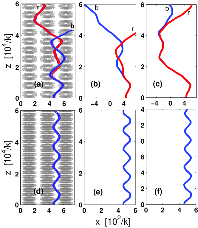
Figure 1: Graph (a): contour plots of the electric field envelope ${\cal E}(x,z)$ solution of NLS (3) in the potential (4) with initial conditions (5) for two slightly different values of the injection point $x_{0}=460$ for the red (r) ray and $x_{0}=461$ for the blue (b) one. The refractive index landscape (4) is plotted for reference. Graph (b) is the driven pendulum approximation (13) and graph (c)is the Eikonal model (15), both simulated with the same initial conditions ($A=2$ in all of those three cases). The lower graphs (d), (e) and (f) describe corresponding simulations with same initial conditions and parameters except for the longitudinal modulation $\Omega$ replaced with $2\Omega$ (then here $A=0.5$).

Our purpose here is to present the first discovery of erratic light rays that occur in a smoothly periodic optical lattice obtained as in kivshar111 by modulation of the refractive index in the two spatial directions. Moreover the modulation along the direction of propagation will be assumed smoother than the transverse one leading then to a quasi two-dimensional problem.

Then we propose a new approach to the spatial soliton description where the effect of lattice grating is considered as a two-wave nonresonant interaction. We show that the chaotic motion is simply related to the parametric driven pendulum which possesses periodic and chaotic regimes, instances of which are presented in fig.1 and obtained by changing the longitudinal modulation length of the optical lattice. Last but not least, this behavior is demonstrated to follow the rules of light ray optics (eikonal) which actually applies thanks to compensation of diffraction by nonlinearity.

The Maxwell’s equations in a non-magnetic film belonging to the $(x,z)$-plane is written hereafter for the out of plane linearly polarized electric field component $E(x,z,t)$ by assuming instantaneous response of the Kerr medium of susceptibility $\chi$:

$$\left(\frac{\partial^{2}}{\partial x^{2}}+\frac{\partial^{2}}{\partial z^{2}}\right)E-\frac{1}{c^{2}}\frac{\partial^{2}}{\partial t^{2}}\left\{n^{2}E+\chi E^{3}\right\}=0.$$ (1)

The linear refractive index variations in the plane result from the optical lattice, thus $n=n(x,z)$. The $z$-axis is chosen along the incident propagation direction and the standard approach to spatial solitons then consists in assuming slowly varying envelope, namely

$$E=\sqrt{2/3}\,{\cal E}(\varepsilon x,\varepsilon^{2}z)e^{i[\omega t-kz]}+c.c.+{\cal O}(\varepsilon^{2}).$$ (2)

with wave number $k=n_{{}_{0}}\omega/c$, where $n_{{}_{0}}$ is a reference refractive index. The small expansion parameter $\varepsilon$ follows from the smallness of the nonlinear Kerr coefficient, thus one may simply define $\chi=\varepsilon^{2}$. Moreover we are interested here in the physical situation when the spatial variations of the refractive index are also weak, namely $n_{{}_{0}}-n(x,z)={\cal O}(\varepsilon^{2})$. In such a case the Maxwell equation (1) in the leading order reduces to the NLS equation ($\varepsilon$ is scaled off)

$$-i\frac{\partial{\cal E}}{\partial z}+\frac{1}{2}\frac{\partial^{2}{\cal E}}{\partial x^{2}}+\chi|{\cal E}|^{2}{\cal E}-\frac{n_{{}_{0}}-n(x,z)}{n_{{}_{0}}}{\cal E}=0,$$ (3)

which is written in dimensionless space variables by the use of new coordinates $z\to kz$ and $x\to kx$. By assuming different scalings along the propagation direction $z$ and transverse direction $x$, the grating index actually defines a quasi two-dimensional lattice, leading then to the above spatial 1+1 dimensional equation in the external potential $1-n/n_{{}_{0}}$.

So far nothing has been assumed for the relative dimensions of the optical lattice wavelength v.s. spatial soliton extension. As a matter of fact preceding works as kevrekidisGrating ; mandelikGap ; ledererGrating consider the case when the spatial soliton sees at least a few periods of the lattice while here we are interested in the case when the lattice modulation varies slowly with respect to the typical soliton size.

To set an example let us assume a lattice periodic in both directions

$$n(x,z)=n_{{}_{0}}\big{[}1-\chi V_{{}_{0}}\sin^{2}(Kx)\sin^{2}(\Omega z)\big{]}.$$ (4)

with $0<\chi V_{{}_{0}}\ll 1$ such that $n_{{}_{0}}-n(x,z)$ is always positive. Then we choose initial conditions for (3) representing the injection of a laser beam in the $z$-direction,

$${\cal E}(x,0)=a\,\textrm{sech}\left[a\sqrt{\chi}\ (x-x_{0})\right]$$ (5)

obtained from the exact soliton solution of (3) for $n=n_{{}_{0}}$. The fig.1(a) now displays two numerical simulations of (3) with

$$a=0.9,\quad\chi=0.01,\quad V_{{}_{0}}=0.2,\quad K=\sqrt{\chi}\pi/25,\quad\Omega=K\sqrt{\chi V_{{}_{0}}},$$ (6)

and two very close initial injection points $x_{0}=460$ (red ray) and $x_{0}=461$ (blue ray). The two spatial soliton rays are plotted against the potential $1-n/n_{{}_{0}}$ for reference. Therefore two very close initial positions result in very different trajectories indicating a chaotic nature of the soliton rays (note the trajectories destabilize although $x_{0}$ is in a region where the external potential vanishes). If now we increase $\Omega$, keeping all other parameters values, we obtain a regime of a periodic stable trajectory presented in fig.1(d).

We propose hereafter a comprehensive interpretation of such a behavior in terms of the equation of the parametric driven pendulum. Our approach is to consider the Maxwell equation (1) where the light beam interacts with the index variations as a fundamental long-wave short-wave nonresonant interaction process. To that end we reconsider the reductive expansion method by following oikawa and seek a solution as

$$E=\varepsilon\sqrt{\frac{2}{3\chi}}\,\Psi(\xi_{1},\zeta)e^{i\theta(\xi_{2},\zeta)}e^{i[\omega t-kz]}+c.c.+\cdots,$$

$$(n(x,z)-n_{{}_{0}})/n_{{}_{0}}=\varepsilon^{2}V(\xi_{2},\zeta)$$

$$\xi_{1}=\varepsilon\left[x-\phi(\xi_{2},\zeta)\right],\quad\xi_{2}=\varepsilon^{2}x,\quad\zeta=\varepsilon^{2}z.$$ (7)

The property that the index variations are smooth with respect to the spatial soliton size is contained in the specific dependences on the slow variable $\xi_{1}$ and very slow variable $\xi_{2}$. The resulting equation at order $\varepsilon^{3}$ appears with terms that depend solely on a single variable, $\Psi(\xi_{1},\zeta)$ on the one side, $\theta(\xi_{2},\zeta)$ and $V(\xi_{2},\zeta)$ on the other side. These terms thus decouple to eventually give

$$\ -i\frac{\partial\Psi}{\partial\zeta}+\frac{1}{2}\frac{\partial^{2}\Psi}{\partial\xi_{1}^{2}}+\big{|}\Psi\big{|}^{2}\Psi=0,\quad\frac{\partial\theta}{\partial\zeta}=-V.$$ (8)

It appears therefore that the effect of the optical lattice, through $V(\xi_{2},\zeta)$, is not an external potential as in (3) but is contained in the coordinate drift $\phi(\xi_{2},\zeta)$ defining $\xi_{1}$. Considering now (1) at order $\varepsilon^{4}$ we get

$$\frac{\partial\phi}{\partial\zeta}=-\frac{\partial\theta}{\partial\xi_{2}}.$$ (9)

We eliminate first the phase $\theta$ between (8) and (9), and second we turn back to initial spatial variables $x$ and $z$ to get

$$\frac{\partial^{2}\phi}{\partial z^{2}}=\frac{1}{n_{{}_{0}}}\frac{\partial n(x,z)}{\partial x}.$$ (10)

Then the nature of equation (8) allows us to start with an explicit spatial soliton solution (in physical dimensions)

$$\Psi_{s}=ae^{-\frac{i}{2}a^{2}\chi z}\,\textrm{sech}\left[a\sqrt{\chi}\,(x-\phi)\right]$$ (11)

whose position $x_{s}(z)$ is thus given by $x_{s}-\phi(x_{s},z)={\rm const}$. To compute the “acceleration” $d^{2}x_{s}/dz^{2}$ we must remember that $\phi$ is slowly varying in $x$ and $z$ and thus keep only the dominant orders, thus

$$\frac{d^{\,2}x_{s}}{dz^{2}}\simeq\frac{\partial^{2}\phi(x_{s},z)}{\partial z^{2}}=\frac{1}{n_{{}_{0}}}\frac{\partial n(x_{s},z)}{\partial x_{s}},$$ (12)

where the last relation follows from (10). This is the Newton law in the “time” $z$ for a particle of unit mass and position $x_{s}$ in the time-dependent potential $-n(x_{s},z)/n_{{}_{0}}$.

Considering now the example (4) used for the simulation in fig.1, the trajectory (12) becomes the following parametrically driven pendulum model pend1 ; pend2

$$\frac{d^{\,2}q}{dt^{2}}=-A\sin^{2}(t)\,\sin(q),\quad A=2\chi V_{{}_{0}}\frac{K^{2}}{\Omega^{2}}$$ (13)

where we have introduced a time $t=\Omega z$ and angle $q(t)=2Kx_{s}(z)$. These reduced units show that the main control parameter is the above defined driving amplitude $A$. The parametric instability of the pendulum with initial angle $q(0)=0$ and velocity $\dot{q}(0)=0$ occur in the range $4/3<A<4$, while the instability fastest growing rate is reached for $A=16[\left(2/\sqrt{3}\right)\,-1]$. However for different initial conditions, chaotic behavior may appear at smaller (or larger) values of $A$ pend1 ; pend2 . The graphs (b) and (e) in fig.1 show the result of simulations of (13) with $A=2$ and $A=0.5$, respecively for initial velocity $\dot{q}(0)=0$ and initial angles corresponding to the rescaled positions of the injected beams. The two different regimes presented result simply from a modification of the modulation period of the lattice along the propagation direction $z$. We observe indeed qualitative agreement, although trajectories should not be quantitatively compared since the regime is chaotic.

In such solitonic regimes, nonlinearity compensates diffraction and the resulting light ray is a good candidate to geometric optics. As a matter of fact we demonstrate that the obtained soliton light ray equation (12) can also be viewed as the eikonal of a light ray in a medium with variable index $n(x,z)$. The eikonal equation written for the position $\vec{r}=(x,z)$ in the plane reads born-wolf

$$\frac{d}{ds}\left(n\frac{d\vec{r}}{ds}\right)=\vec{\nabla}n,$$ (14)

where $s$ is the arc length, namely $ds^{2}=dx^{2}+dz^{2}$. We write this equation for the ray $x=x(z)$ as we did for the soliton motion, and obain after some algebra that the above two components reduce to ($x^{\prime}=dx/dz$)

$$x^{\prime\prime}=[1+(x^{\prime})^{2}]\frac{1}{n}\,\left(\frac{\partial n}{\partial x}-x^{\prime}\,\frac{\partial n}{\partial z}\right),$$ (15)

where the right hand side is eveluated on the trajectory $x=x(z)$. To recover the soliton light ray, we must now use the assumption $x^{\prime}\ll 1$, which is precisely the assumption made to obtain the NLS equation (3) from Maxwell equation (1). Taking also into account that $n(x,z)-n_{{}_{0}}\ll n_{{}_{0}}$ one readily obtains from (15)

$$x^{\prime\prime}\simeq\frac{1}{n_{{}_{0}}}\,\frac{\partial n}{\partial x},$$ (16)

which is just the trajectory equation (12). Numerical simulations of (15) have been performed for the same parameter values as precedingly (initial postion $x_{0}$, vanishing initial veleocities and explicit expression of $n(x(z),z)$). The result is plotted in fig.1(c) and fig.1(f), which confirms consistency with prediction of geometric optics.

It is remarkable that such different models as NLS (3) in the external potential smoothly modulated in both spatial directions and the driven parametric pendulum (13) concur to describe trajectory of a spatial soliton in a smoothly modulated (1+1) dimensional lattice. It is also striking that the soliton ray actually follows the rule of geometric optics in this context, which opens interesting perspectives on both theoretical and experimental aspects.

One practical advantage of the parametric pendulum description is the prediction of the switching from regular to chaotic (erratic) trajectories of the spatial soliton. This result might be useful for conceiving all optical ultrasensitive noise amplifiers. Last, our result is expected to apply to the case of Bose-Einstein condensate with attractive nonlinearity in smooth space and time dependent optical lattices, for which a similar dynamics will occur but there in the time domain.

We are grateful to D. Felbacq and B. Guizal for enlighting dicussions. Work done under contract CNRS GDR-3073. R.K. aknowledges stay as invited professor at the Laboratoire de Physique Théorique et Astroparticules and financial support of the Georgian National Science Foundation (Grant No GNSF/STO7/4-197).

References

- (1) Y.S. Kivshar, G.P. Agrawal, “Optical Solitons: From Fibers to Nonlinear Crystals”, Academic Press (London, 2003).
- (2) M. Segev, G. Stegeman, “Self Trapping of optical beams: Spatial soliton”, Phys. Today, 51 (1998) 42; M. Mitchell, M. Segev, “Self-trapping of incoherent white light”, Nature 387 (1997) 880.
- (3) M. Segev, G. C. Valley, B. Crosignani, P. D. Porto, and A. Yariv, “Steady-state spatial screening solitons in photorefractive materials with external applied field”, Phys. Rev. Lett. 73 (1994) 3211.
- (4) D.N. Christodoulides, M.I. Carvalho, “Bright, dark, and gray spatial soliton states in photorefractive media”, J. Opt. Soc. Am. B 12 (1995) 1628.
- (5) J.S. Aitchison, A.M. Weiner, Y. Silberberg, D.E. Leaird, M.K. Oliver, J.L. Jackel, P.W.E. Smith, “Experimental-observation of spatial soliton-interactions”, Opt. Lett. 16 (1991) 15.
- (6) W. Krolikowski, S.A. Holmstrom, “Fusion and birth of spatial solitons upon collision”, Opt. Lett. 22 (1997) 369.
- (7) A.W. Snyder, A.P. Sheppard, “Collisions, steering, and guidance with spatial solitons”, Opt. Lett. 18 (1993) 482.
- (8) O. Cohen, R. Uzdin, T. Carmon, J.W. Fleischer, M. Segev, S. Odoulov, “Collisions between optical spatial solitons propagating in opposite directions”, Phys. Rev. Lett. 89 (2002) 133901.
- (9) D. Song, C. Lou, L. Tang, X. Wang, W. Li, X. Chen, K.J.H Law, H. Susanto, P.G. Kevrekidis, J. Xu, Z. Chen, “Self-trapping of optical vortices in waveguide lattices with a self-defocusing nonlinearity”, Opt. Express, 16 (2008) 10110.
- (10) D. Mandelik, R. Morandotti, J.S. Aitchison, Y. Silberberg, “Gap solitons in waveguide arrays”, Phys. Rev. Lett. 92 (2004) 093904.
- (11) A. Szameit, Y.V. Kartashov, F. Dreisow, M. Heinrich, T. Pertsch, S. Nolte, A. Tunnermann, V.A. Vysloukh, F. Lederer, L. Torner, “Inhibition of Light Tunneling in Waveguide Arrays”, Phys. Rev. Lett. 102 (2009) 153901.
- (12) E.M. Gromov, “Propagation of short nonlinear wave packets and solitons in smoothly inhomogeneous media”, Phys. Lett. A 227 (1997) 67.
- (13) Y. Sivan, G. Fibich, N.K. Efremidis, S. Bar-Ad, “Analytic theory of narrow lattice solitons”, Nonlinearity 21 (2008) 509.
- (14) K. Staliunas, O. Egorov, Y. Kivshar, F. Lederer, “Bloch Cavity Solitons in Nonlinear Resonators with Intracavity Photonic Crystals”, Phys. Rev. Lett. 101 (2008) 153903.
- (15) M. Oikawa, N. Yajima, “Perturbation approach to nonlinear-systems. 2 Interaction of nonlinear modulated waves”, J. Phys. Soc. Japan 37 (1974) 486.
- (16) J. Starrett, R. Tagg, “Control of a chaotic parametrically driven pendulum”, Phys. Rev. Lett. 74 (1995) 1974.
- (17) A.D. Churukian, D.R. Snider, “Finding the windows of regular motion within the chaos of ordinary differential equations”, Phys. Rev. E 53 (1996) 74.
- (18) M. Born, E. Wolf, “Principles of Optics”, University Press (Cambridge 2002).