Coulomb-modified Fano interference in a double quantum dot Aharonov-Bohm ring

Abstract

In this paper, the Coulomb-induced changes of Fano interference in electronic transport through a double quantum dot Aharonov-Bohm ring are discussed. It is found that the Coulomb interaction in the quantum dot in the reference channel can remarkably modify the Fano interference, including the increase or decrease of the symmetry of the Fano lineshape, as well as the inversion of the Fano lineshape, which is dependent on the appropriate strength of the Coulomb interaction. When both the quantum dot levels are adjustable, the Coulomb-induced splitting of the nonresonant channel leads to the destruction of the Fano interference; whereas two blurry Fano lineshapes may appear in the conductance spectra when the many-body effect in the dot of the resonant channel is also considered. Interestingly, in the absence of magnetic field, when the different-strength electron interactions make one pair of levels of the dots in different channels the same, the corresponding resonant state keeps vacuum despite the adjustment of quantum dot levels.

I Introduction

The Fano effect, arising from the quantum interference between resonant and nonresonant processes,refFano ; Andrey has been observed in various physical fields, including neutron scattering,Adair atomic photoionization,Fano2 Raman scattering,Cardona optical absorption in quantum wells,Faist scanning tunneling microscopy,Chen and microwave scattering.Rotter As a result, asymmetric lineshapes appear in the spectra concerned, e.g., optical absorption spectrum, usually called the Fano lineshapes.Andrey ; Faist Quantum dots (QDs), in particular, the coupled multiple QD structures, provide multiple channels for electronic coherent transmission. In appropriate parameter region, one or a few channels serve as the resonant paths for electron tunneling and the others are the nonresonant ones. Quantum interference of electron waves going through these different paths inevitably leads to the occurrence of Fano effect in the electron transport through these structures.

Experimentally, Fano resonances have been observed first in QDs at the Kondo regime.Gores ; Gordon Subsequently, by embedding a Coulomb blockaded QD in an Aharonov-Bohm (AB) ring interferometer, a variety of Fano lineshapes were observed in the measured conductance spectra. Conductance measurements exploring different geometries, such as a quantum wire with a side-coupled QD,refIye ; refWang ; refTor a one-lead QD,Hanson a ring with side-coupled QD,Fuhrer as well as the parallel double QD structures,Blick ; Chen2 provide more insight into the Fano problem in mesoscopic systems.

The occurrence of conductance dips in ballistic AB rings was theoretically investigated almost 20 years ago.Weisz Further, early theoretical works examined the possibility of Fano lineshapes in the transmission through one-dimensional waveguides and waveguides with resonantly coupled cavities.Tekman Recently, inspired by the development of the relevant experimental works, there have been a lot of theoretical investigations devoting themselves to the Fano interference in electron transport through various QD structures, for example, one or two QDs embedded in an AB ring,refBulka ; refKonig1 ; refKonig2 ; refGefen double QDs in different coupling manners.refKang ; refBai ; refOrellana ; refZhu ; refDing According to these theoretical results, the Fano effect in QD structures exhibits some peculiar behavoirs in electronic transport process, in contrast to the conventional Fano effect. These include the tunable Fano lineshape by the magnetic or electrostatic fields applied on the QDs,refKang ; refBai ; refOrellana ; refZhu the Kondo resonance associated Fano effect,refBulka ; refKonig1 ; refDing ; refMeden Coulomb-modification on the Fano effect,refZhu2 the impurity-influenced Fano interference,gongjap the relation between the dephasing time and the Fano parameter $q$,refClerk and the spin-dependent Fano interference when various spin-relevant field is applied.Chi

According to these previous works, since the understanding of the important role of Coulomb interactions in electron transport through the coupled-QD structures, in so many previous literatures,refBulka ; refKonig1 ; refDing ; refMeden when the Fano interference in electron tunneling through the corresponding QD structures were investigated, the influence of the many-body effect on the Fano resonance is always a leading concern. Albeit these theoretical descriptions, some aspects about the Coulomb-modified Fano effect in QD structures deserve further theoretical investigation. First, we have to know that in the mixed-valence regime, the Coulomb interactions also contribute nontrivially to the electron transport process, since the quantum interference is modified by the Coulomb-induced splitting of the QD levels (Interpretatively, $\varepsilon_{0}$ is changed into $\varepsilon_{0}$ and $\varepsilon_{0}+U$ with $\varepsilon_{0}$ being one QD level and $U$ the Coulomb interaction strength). Accordingly, the Coulomb-induced multi-channel quantum interference presents some complicated properties quite different from those in the noninteracting case. Such an issue was discussed in the model of parallel-coupled double QDs, in which the observable change of the Fano effect is exhibited.refZhu2 Secondly, as is known, with respect to the multi-QD structures, such as the double-QD AB ring, it is not necessary that there are equal electron interactions in the respective QDs.Silva Thereby, the investigation of the influence of the unequal Coulomb repulsions on the quantum interference, e.g., the Fano interference, is desirable.

Motivated by such a topic, in this work we concentrate our attention on the Coulomb-modified Fano effect in electronic transport through a double-QD AB ring. Then, with the help of the standard Fano form of the linear conductance expression, the Coulomb-induced changes of the Fano lineshapes in the linear conductance spectra are discussed in detail. It is found that the Coulomb interaction in the QD in the reference channel plays a nontrivial role in the change of the Fano lineshapes. For the case of the adjustable levels of both QDs, the Coulomb-induced splitting of the nonresonant channel leads to the destruction of the Fano interference. Only when the many-body effect in both QDs of the ring, blurry Fano lineshapes are possible to appear in the conductance spectra. In addition, in the zero-magnetic-field case, when the different-strength electron interactions make any pair of QD levels of different channels consistent, the corresponding resonant state keeps vacuum.

The rest of the paper is organized as follows. In Sec. II, the model Hamiltonian to describe the electron motion in double-QD AB ring is introduced firstly. Then a formula for the linear conductance is derived by means of the nonequilibrium Green function technique and the Fano form of the conductance expression are obtained. In Sec. III, the calculated results about the linear conductance spectrum are shown. Then a discussion focusing on the change of Fano lineshape is given. Finally, the main results are summarized in Sec. IV.

II model

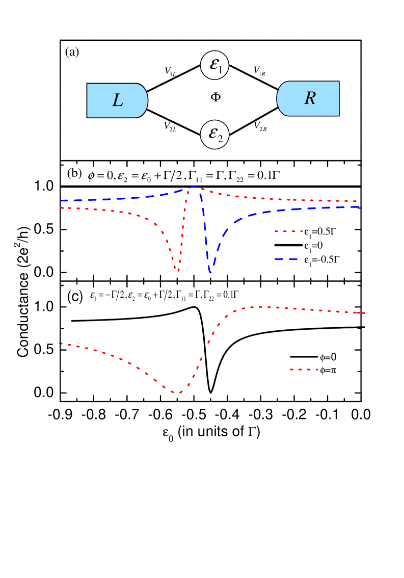
Figure 1: (a) Schematic of a double-QD AB interferometer. (b) The linear conductance spectra with $\varepsilon_{1}=\frac{1}{2}\Gamma$, $0$, and $-\frac{1}{2}\Gamma$, respectively, in the absence of magnetic field. (c) The compared conductance spectra for the cases of $\phi=0$ and $\pi$ with $\varepsilon_{1}=-\frac{1}{2}\Gamma$. The QD-lead couplings are $\Gamma_{11}=10\Gamma_{22}=\Gamma$ and and the level of QD-2 $\varepsilon_{2}=\varepsilon_{0}+\frac{1}{2}\Gamma$.

The double-QD AB ring we consider is illustrated in Fig. 1(a). The Hamiltonian to describe the electronic motion in this structure reads $H=H_{C}+H_{D}+H_{T}$. The first term is the Hamiltonian for the noninteracting electrons in the two leads:

$$H_{C}=\underset{\sigma,k,\alpha\in L,R}{\sum}\varepsilon_{\alpha k}c_{\alpha k\sigma}^{\dagger}c_{\alpha k\sigma},$$ (1)

where $c_{\alpha k\sigma}^{\dagger}$ $(c_{\alpha k\sigma})$ with $\sigma=\pm 1$ (or $\uparrow,\downarrow$) being the spin index is an operator to create (annihilate) an electron of the continuous state $|k,\sigma\rangle$ in lead-$\alpha$, and $\varepsilon_{\alpha k}$ is the corresponding single-particle energy. The second term describes electron in the two QDs in the arms of the ring, which takes a form as

$$H_{D}=\sum_{j=1,\sigma}^{2}\varepsilon_{j}d_{j\sigma}^{\dagger}d_{j\sigma}+\sum_{j=1}^{2}U_{j}n_{j\uparrow}n_{j\downarrow},$$ (2)

where $d^{{\dagger}}_{j\sigma}$ $(d_{j\sigma})$ is the creation (annihilation) operator of electron in QD-$j$. And $\varepsilon_{j}$ denotes the electron level in the corresponding QD, while $U_{j}$ represents the intradot Coulomb repulsion. We assume that only one level is relevant in each QD. The last term in the Hamiltonian describes the electron tunneling between the leads and QDs. It is given by

$$H_{T}=\underset{jk,\sigma}{\sum}(V_{j{\scriptscriptstyle L}}d_{j\sigma}^{\dagger}c_{{\scriptscriptstyle L}k\sigma}+V_{j{\scriptscriptstyle R}}d_{j\sigma}^{\dagger}c_{{\scriptscriptstyle R}k\sigma}+\mathrm{H.c.}),$$ (3)

where $V_{j\alpha}$ denotes the QD-lead coupling strength. The tunnelling matrix elements take the following values: $V_{1{\scriptscriptstyle L}}=|V_{1{\scriptscriptstyle L}}|e^{i\phi/4}$, $V_{1{\scriptscriptstyle R}}^{*}=|V_{1{\scriptscriptstyle R}}|e^{i\phi/4}$, $V_{2{\scriptscriptstyle R}}=|V_{2{\scriptscriptstyle R}}|e^{i\phi/4}$, and $V_{2{\scriptscriptstyle L}}^{*}=|V_{2{\scriptscriptstyle L}}|e^{i\phi/4}$. The phase shift $\phi$ is associated with the magnetic flux $\Phi$ threading the system by a relation $\phi=2\pi\Phi/\Phi_{0}$, in which $\Phi_{0}=h/e$ is the flux quantum.

To study the electronic transport properties in the linear regime, the linear conductance at zero temperature is obtained by the Landauer-Büttiker formularefLandauer ; refMeir1

$$\mathcal{G}=\frac{e^{2}}{h}\sum_{\sigma}T_{\sigma}(\omega)|_{\omega=\varepsilon_{F}}.$$ (4)

$T_{\sigma}(\omega)$ is the transmission function, in terms of Green function which takes the form as $T_{\sigma}(\omega)=\mathrm{Tr}[\Gamma^{L}G^{r}_{\sigma}(\omega)\Gamma^{R}G^{a}_{\sigma}(\omega)]$, where $\Gamma^{L}$ is a $2\times 2$ matrix and defined as $[\Gamma^{L}]_{jn}=2\pi V_{j{\scriptscriptstyle L}}V^{*}_{n{\scriptscriptstyle L}}\rho_{\scriptscriptstyle L}(\omega)$, describing the coupling strength between the two QDs and lead-$L$. We will ignore the $\omega$-dependence of $\Gamma^{L}_{jn}$ since the electron density of states in lead-$L$, $\rho_{\scriptscriptstyle L}(\omega)$, can be usually viewed as a constant. By the same token, we can define $[\Gamma^{R}]_{jn}$. Besides, the retarded and advanced Green functions in Fourier space are involved here. By means of the equation-of-motion method and via a straightforward derivation,refGong we obtain the retarded Green functions written in a matrix form:

$$G^{r}_{\sigma}(\omega)=\left[\begin{array}[]{cc}g_{1\sigma}(z)^{-1}&i\Gamma_{12}\\ i\Gamma_{21}&g_{2\sigma}(z)^{-1}\end{array}\right]^{-1}\ ,$$ (7)

with $z=\omega+i0^{+}$. And $g_{j\sigma}(z)=[(z-\varepsilon_{j})\Lambda_{j\sigma}+i\Gamma_{jj}]^{-1}$, is the zero-order Green function of the QD-$j$ unperturbed by another QD, where $\Gamma_{jn}={1\over 2}\{[\Gamma^{L}]_{jn}+[\Gamma^{R}]_{jn}\}$. Besides,

$$\Lambda_{j\sigma}=\frac{z-\varepsilon_{j}-U_{j}}{z-\varepsilon_{j}-U_{j}+U_{j}\langle n_{j\bar{\sigma}}\rangle}$$ (8)

results from the second-order approximation (i.e., Hubbard approximation) for Coulomb terms.refGong ; refLiu The average electron occupation number in QD-$j$ is determined by the relation $\langle n_{j\sigma}\rangle=\frac{i}{2\pi}\int d\omega[{G}^{<}_{\sigma}(\omega)]_{jj}$, in which ${G}^{<}_{\sigma}(\omega)={G}^{r}_{\sigma}(\omega)\Sigma^{<}{G}^{a}_{\sigma}(\omega)$ with $\Sigma^{<}=i\Gamma^{L}f_{L}+i\Gamma^{R}f_{R}$. In addition, the advanced Green function can be readily obtained via a relation $G_{\sigma}^{a}(\omega)=[G_{\sigma}^{r}(\omega)]^{\dagger}$.

With the solution of the Green function and the definition of the coupling matrixes $\Gamma^{\alpha}$, we can express the linear conductance defined by Eq.(4) in terms of the structure parameters, i.e.,

$$\mathcal{G}=\frac{e^{2}}{h}\sum_{\sigma}\frac{\tilde{\varepsilon}^{2}_{2\sigma}\Gamma^{L}_{11}\Gamma^{R}_{11}+\tilde{\varepsilon}^{2}_{1\sigma}\Gamma^{L}_{22}\Gamma^{R}_{22}+\tilde{\varepsilon}_{1\sigma}\tilde{\varepsilon}_{2\sigma}(\Gamma^{L}_{12}\Gamma^{R}_{21}+\Gamma^{L}_{21}\Gamma^{R}_{12})}{(\tilde{\varepsilon}_{1\sigma}\tilde{\varepsilon}_{2\sigma}-\Gamma_{11}\Gamma_{22}+\Gamma_{12}\Gamma_{21})^{2}+(\Gamma_{11}\tilde{\varepsilon}_{2\sigma}+\Gamma_{22}\tilde{\varepsilon}_{1\sigma})^{2}},$$ (9)

with $\tilde{\varepsilon}_{j\sigma}=\varepsilon_{j}\Lambda_{j\sigma}$ being the renormalized level of QD-$j$. The expression corresponds to Eq. (9) in the work of C. Karrasch $et$ $al.$refMeden distinctly. In order to study the Fano interference, one usually rewrites the conductance expression into a Fano form, i.e.,

$$\mathcal{G}=\frac{e^{2}}{h}\sum_{\sigma}T_{b\sigma}\frac{|e_{\sigma}+q_{\sigma}|^{2}}{e^{2}_{\sigma}+1},$$ (10)

in which the three auxiliary quantities are defined as $T_{b\sigma}=\Gamma^{L}_{11}\Gamma^{R}_{11}/[|\tilde{\varepsilon}_{1\sigma}|^{2}+\Gamma^{2}_{11}]$, $e_{\sigma}=-\mathrm{Re}G^{r}_{22,\sigma}/\mathrm{Im}G^{r}_{22,\sigma}$, and $q_{\sigma}=-\frac{\tilde{\varepsilon}_{1\sigma}}{\Gamma_{11}}(\Gamma^{L}_{12}\Gamma^{R}_{21}\Gamma_{11}-T_{b\sigma}\Gamma_{12}\Gamma_{21}\Gamma_{11})/({\Gamma^{L}_{11}\Gamma^{R}_{11}\Gamma_{22}-T_{b\sigma}\Gamma_{12}\Gamma_{21}\Gamma_{11}})$. Obviously, $T_{b\sigma}$ is the ability of electron transmission through the upper arm of the ring. Under the condition of symmetric QD-lead coupling, $\Gamma^{L}_{jj}=\Gamma^{R}_{jj}$, so $q_{\sigma}$ can be simplified as $q_{\sigma}=-\frac{\tilde{\varepsilon}_{1\sigma}}{\Gamma_{11}}(e^{i\phi}-T_{b\sigma}\cos^{2}\frac{\phi}{2})/(1-T_{b\sigma}\cos^{2}\frac{\phi}{2})$. Also, from Eq.(10) we can find that Fano antiresonance emerges while $e_{\sigma}+q_{\sigma}=-[\Gamma^{L}_{11}\Gamma^{R}_{11}\tilde{\varepsilon}_{2\sigma}+\Gamma^{L}_{12}\Gamma^{R}_{21}\tilde{\varepsilon}_{1\sigma}]/[4\Gamma^{L}_{11}\Gamma^{R}_{11}\Gamma_{22}-T_{b\sigma}\Gamma_{11}\Gamma_{12}\Gamma_{21}]=0$, which indicates that Fano antiresonance emerges inevitably while $\Gamma^{L}_{11}\Gamma^{R}_{11}\tilde{\varepsilon}_{2\sigma}+\Gamma^{L}_{12}\Gamma^{R}_{21}\tilde{\varepsilon}_{1\sigma}=0$.

III Numerical results and discussions

Based on the formulation developed in the previous section, we can then carry out the numerical calculation to investigate the Fano interference in electron transport through such a double-QD AB ring structure. Before proceeding, we consider $\Gamma$ as the unit of energy and take the Fermi level of the system $\varepsilon_{F}$ as the zero point of energy.

First, with the help of a standard Fano expression Eq.(10), by analyzing the Fano parameter $q_{\sigma}$ we can investigate the appearance of the Fano lineshape in the linear conductance spectrum. It is certain that when $q_{\sigma}$ is real, the linear conductance is possible to display a standard Fano lineshape, and moreover the change of the sign of $q_{\sigma}$ ($+/-$) can lead to the reversal of the Fano lineshape. As discussed in the previous works,refOrellana ; refZhu ; gongpe there are two ways to realize the change of the sign of $q_{\sigma}$, i.e., by choosing the different-sign values of the level of QD-1 with respect to the Fermi level or tuning the threading magnetic flux from $\phi=2n\pi$ to $\phi=(2n+1)\pi$ ($n\in Integer$). As shown in Fig.1(b) and (c), when the level of QD-1 is fixed at a nonzero value with respect to the Fermi level, the upper arm of the AB ring accordingly provides a reference (nonresonant) channel for the Fano interference, consequently, with the shift of the level of QD-2 the calculated conductance spectra present the Fano lineshapes apparently. To be concrete, in the absence of magnetic flux, $q_{\sigma}$ is equal to $-{\varepsilon_{1}\over\Gamma_{11}}$, thereby, the opposite-sign values of QD-1 level causes the opposition of signs ($+/-$) of $q_{\sigma}$, which gives rise to the inversion of the Fano lineshape. Of course, $\varepsilon_{1}=0$, implying $q_{\sigma}=0$, is a critical position of the lineshape’s inversion, correspondingly, in such a case the liner conductance is equal to $2e^{2}/h$, independent of the modulation of $\varepsilon_{2}$. On the other hand, when the magnetic flux increases to $\pi$, the Fano parameter $q_{\sigma}$ has the expression $q_{\sigma}={\varepsilon_{1}\over\Gamma_{11}}$, hence the Fano lineshape can also be inverted despite $\varepsilon_{1}=-{\Gamma\over 2}$ fixed, as shown in Fig.1(c).

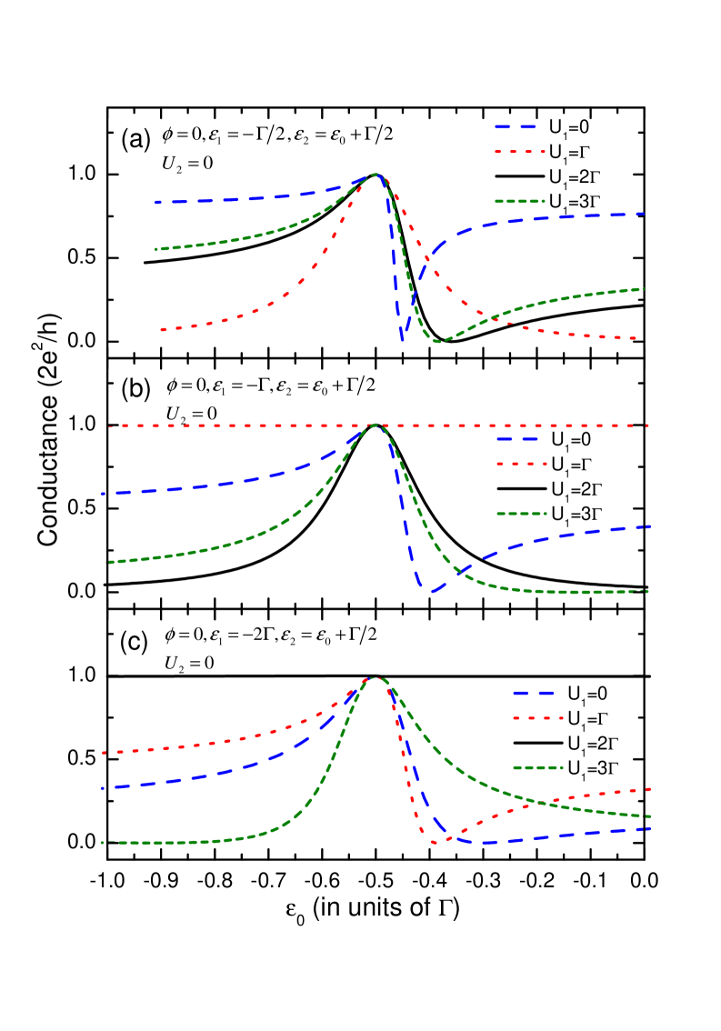
Figure 2: The conductance spectra influenced by the different-strength Coulomb repulsions in QD-1, with the level of QD-1 being respectively fixed at $-0.5\Gamma$, $-\Gamma$, and $-2\Gamma$.

Next, we turn to pay attention to the influence of the many-body effect on the change of the Fano lineshape. It is known that the many-body effect is an important origin for the peculiar transport properties in coupled-QD structures. Therefore, it is supposed to influence the Fano resonance to some extent. Usually, the many-body effect is incorporated by considering only the intradot Coulomb repulsion, i.e., the Hubbard term. In general, if the Hubbard interaction is not very strong, we can truncate the equations of motion of the Green functions to the second order.refGong ; refLiu In Figs.2, by choosing $U_{2}=0$ and $\varepsilon_{2}=\varepsilon_{0}+{\Gamma\over 2}$, we first investigate the influence of the many-body effect in QD-1 on the Fano interference and plot the Coulomb-modified linear conductance spectra as functions of $\varepsilon_{2}$. From the figure, we can readily see that the increase of Coulomb repulsion strength of QD-1 indeed changes the Fano lineshape in a nontrivial way. As a typical case, in Fig.2(a) with $\varepsilon_{1}=-{\Gamma\over 2}$, when $U_{1}=\Gamma$ it is interesting that the conductance spectrum presents a Breit-Wigner lineshape with its resonant peak at the point of $\varepsilon_{2}=0$, corresponding to the dotted line in this figure. This indicates that in such a case, only the electron transport through the down arm of the ring is allowed, so that the Fano interference vanishes completely. With the increment of the Coulomb strength, such as for the cases of $U_{1}=2\Gamma$ and $3\Gamma$, the conductance profiles show themselves as the Fano lineshapes again, but the asymmetry degree of them is weaker compared with that in the noninteracting case. Next, in the cases of $\varepsilon_{1}=-\Gamma$, as exhibited in Fig.2(b), when $U_{1}=\Gamma$ the corresponding conductance is equal to $2e^{2}\over h$ in the whole range of $\varepsilon_{2}$; but when $U_{1}=2\Gamma$, the linear conductance spectrum gets close to the Breit-Wigner lineshape as well, similar to the result in the case of $\varepsilon_{1}=-{\Gamma\over 2}$ and $U_{1}=\Gamma$. Alternatively, under the condition of $\varepsilon_{1}=-2\Gamma$ it is shown that the increase of $U_{1}$ (i.e., the case of $U_{1}=3\Gamma$) can give rise to the reversal of the Fano lineshape, just as displayed by the shot-dashed line in Fig.2(c). Therefore, by virtue of the above results, the effect of the Coulomb interaction in the reference channel on the Fano interference is striking.

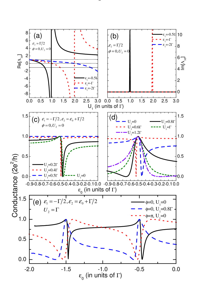
Figure 3: (a) and (b) The curves of $\rm{Re}\Lambda_{1\sigma}$ and $\rm{Im}\Lambda_{1\sigma}$ as functions of $U_{1}$. (c) and (d) The $U_{1}$-modulated conductance spectra. (e) The linear conductance in the presence of nonzero $U_{2}$.

We can find, from Eq.(9), that in the linear transport regime, the many-body effect modify the electron transport through such a structure by renornalizing the QD levels $\varepsilon_{j}$ to $\tilde{\varepsilon}_{j\sigma}=\varepsilon_{j}\Lambda_{j\sigma}=\varepsilon_{j}(i0^{+}-\varepsilon_{j}-U_{j})/(i0^{+}-\varepsilon_{j}-U_{j}+U_{j}\langle n_{j\bar{\sigma}}\rangle)$. Therefore, it is understood that the many-body effect in QD-1 can efficiently adjust the Fano lineshape in the conductance curves with its modulating the Fano parameter $q_{\sigma}$, since in the absence of magnetic flux $q_{\sigma}=-{\varepsilon_{1\sigma}\over\Gamma_{11}}=-{\varepsilon_{1}\over\Gamma_{11}}\Lambda_{1\sigma}$ ( or $q_{\sigma}={\varepsilon_{1\sigma}\over\Gamma_{11}}={\varepsilon_{1}\over\Gamma_{11}}\Lambda_{1\sigma}$ when $\phi=\pi$). In Fig.3(a) and (b), by assuming $\varepsilon_{1}=-{\Gamma\over 2}$, $-\Gamma$, and $-2\Gamma$, the profiles of ${\rm Re}[\Lambda_{1\sigma}]$ and ${\rm Im}[\Lambda_{1\sigma}]$ are plotted as functions of $U_{1}$, respectively. It is seen that in general regime, only the real part of $\Lambda_{1\sigma}$ contributes to the variation of $q_{\sigma}$, whereas when the condition of $U_{1}=2\varepsilon_{1}$ is satisfied, both the real and imaginary parts of $\Lambda_{1\sigma}$ play important roles in the sharp change of $q_{\sigma}$. Taking the case of $\varepsilon_{1}=-{\Gamma\over 2}$ as an example, in the vicinity of $U_{1}=\Gamma$, $|\Lambda_{1\sigma}|$ approximately goes to infinity, so, in such a case $q_{\sigma}\rightarrow\infty$ and then the conductance expression can mathematically be simplified as ${\cal G}={e^{2}\over h}\sum_{\sigma}{1\over e^{2}_{\sigma}+1}={e^{2}\over h}\sum_{\sigma}|g_{2\sigma}|^{2}$, which is according to the display of a Breit-Wigner lineashape in the linear conductance curve. The physical reason of such a result can be clarified as follows. As is known, in the presence of many-body effect, the level of QD-1 splits into two, i.e., $\varepsilon_{1}$ and $\varepsilon_{1}+U_{1}$, thus the consideration of $\varepsilon_{1}=-{\Gamma\over 2}$ and $U_{1}=\Gamma$ gives rise to the electron-hole symmetry of QD-1 and the occupation number of $\sigma$-spin in QD-1 is just $\langle n_{1\sigma}\rangle={1\over 2}$. By virtue of the description in the previous works,refGong we can be sure that the electron-hole symmetry is able to restrain the electron tunneling through the upper arm of the ring, when the electron correlation effect is ignored. As a consequence, in such a case only the electron transmission through the down arm ( resonant channel ) is allowed, which results in the appearance of the Breit-Wigner lineshape in the linear conductance. On the other hand, from Fig.3(a) and (b), it can also be found that when $\varepsilon_{1}=-\Gamma$ and $U_{1}=\Gamma$ is considered, $\Lambda_{1\sigma}$ becomes equal to zero, hence in such a case the Fano parameter $q_{\sigma}=0$ and $e_{\sigma}\rightarrow\infty$, as a result, the conductance is equal to $2e^{2}\over h$ independent of the tuning of $\varepsilon_{2}$. On the other hand, for the case of $\varepsilon_{1}=-2\Gamma$ and $U_{1}=3\Gamma$, one can see that $\Lambda_{1\sigma}$ becomes negative obviously, which results in the inversion of the Fano lineshape in the calculated conductance profile.

Typically, let us continue to devote ourselves to the curve of ${\rm Re}[\Lambda_{1\sigma}]$ and ${\rm Im}[\Lambda_{1\sigma}]$ of $\varepsilon_{1}=-{\Gamma\over 2}$. One can readily find that in the process of $U_{1}$ increasing to $\Gamma\over 2$, ${\rm Re}[\Lambda_{1\sigma}]$ decreases from $1$ to zero, which leads to the decrease of $q_{\sigma}$ ( since here ${\rm Im}[\Lambda_{1\sigma}]=0$ ) and the increase of the asymmetry of the Fano lineshape, corresponding to the results in Fig.3(c). Well, it is clear that $U_{1}={\Gamma\over 2}$ make $q_{\sigma}$ close to infinity, so the conductance becomes a constant irrelevant to the shift of $\varepsilon_{2}$. When the Coulomb repulsion strength exceeds $\Gamma\over 2$ $\rm Re[\Lambda_{1\sigma}]$ becomes negative until the point of $U_{1}=\Gamma$, accordingly the sign of $q_{\sigma}$ changes and such a result brings about the reversal of the Fano lineshape in the calculated linear conductance spectrum, as shown in Fig.3(d). When go on increasing the Coulomb strength in QD-1, we can see that $\rm Re{\Lambda_{1\sigma}}$ always keeps positive with the amplitude of it greater than one, so under such a condition the weak modulation of $U_{1}$ on the Fano lineshape is well understood, too. With the results above, we can clarify the phenomenon of the modulation of many-body effect in QD-1 on the Fano interference in such a system. In addition, it is necessary to point out that when the Coulomb interaction in QD-2 is taken into account, the electron interaction in QD-2 can induce the splitting of the level of QD-2(i.e., $\varepsilon_{2}$ and $\varepsilon_{2}+U_{2}$), so it is clear that the Fano lineshape in the conductance spectrum will be divided into two groups, but the properties of the Fano lineshape are still determined by the Coulomb term in QD-1, as shown in Fig.3(e).

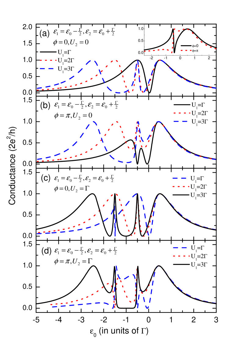
Figure 4: The Coulomb-modified conductance spectra for the cases of the adjustable levels of QD-1 and QD-2. The relevant parameters are taken as $\varepsilon_{1}=\varepsilon_{0}-\frac{1}{2}\Gamma$, $\varepsilon_{2}=\varepsilon_{0}+\frac{1}{2}\Gamma$, and $\Gamma_{11}=10\Gamma_{22}=\Gamma$.

For the case of the adjustable $\varepsilon_{1}$, by letting $\Gamma_{11}=10\Gamma_{22}=\Gamma$ and $\varepsilon_{1}=\varepsilon_{0}-{\Gamma\over 2}$ one can also readily find a Fano lineshape in the linear conductance spectrum, as shown in the inset of Fig.4(a). This is for the reason that here the upper arm of this ring can provide a ‘less’ resonant path while its down arm provides a ‘more’ resonant path for the occurrence of Fano interference. Then, according to the results in Fig.4 (a) and (b), in comparison with that in the noninteracting case, in such a case the existence of the many-body effect in QD-1 can also modify the Fano interference to a great extent. In the absence of magnetic flux and the many-body term in QD-2, as shown in Fig.4(a), we find that when $U_{1}=\Gamma$, in the conductance spectrum there exist two peaks respectively corresponding to the positions of $\varepsilon_{0}={\Gamma\over 2}$ and $-{\Gamma\over 2}$ with the approximately-equal width of them, and at the vicinity of $\varepsilon_{0}=0$ the conductance encounters its zero value. It is therefore certain that in such a case, the original Fano interference disappears completely since the consideration of many-body effect. Such a result can be well explained as follows. Certainly, the Coulomb interaction in the Hubbard approximation can lead to the splitting of the energy level $\varepsilon_{1}$ into $\varepsilon_{1}$ and $\varepsilon_{1}+U_{1}$,refGong ; refLiu so with the adjustment of $\varepsilon_{1}$ in the conductance curve there are two peaks corresponding to the points of $\varepsilon_{1}=0$ and $\varepsilon_{1}+U_{1}=0$, respectively. With respect to the zero point of the conductance, we can understand that it arises from the electron-hole symmetry, as discussed above. But, we have to note that in this case due to $\varepsilon_{2}=\varepsilon_{1}+U_{1}$, the conductance peak at the point of $\varepsilon_{1}+U_{1}=0$ originates from the constructive interference between the electron waves passing through the two arms, since at this position the absence of magnetic flux causes the uniform phase of the electron waves. With the increase of $U_{1}$, there appear three conductance peaks in the linear conductance spectra, respectively associated with the points of $\varepsilon_{1}$, $\varepsilon_{2}$, and $\varepsilon_{1}+U_{1}$ equal to the Fermi level. Apparently, we have to know that owing to the Coulomb-induced splitting of the conductance spectrum in the upper arm, electron transmission though this channel can not be regarded as a ‘less’ resonant process. Therefore, the Fano interference is seriously destroyed and the linear conductance spectrum does not display a standard Fano lineshape any more.

When a local magnetic flux is introduced with $\phi=\pi$, as shown in Fig.4(b), it is found that for the case of $U_{1}=\Gamma$, opposite to the result of zero magnetic field, when $\varepsilon_{2}$ (i.e., $\varepsilon_{1}+U_{1}$) coincides with the Fermi level of the system the electron transport becomes antiresonant. This is because that the application of magnetic field with $\phi=\pi$ gives rise to the opposition of the phases of the electron waves traveling through the two arms, and the destructive interference results in the occurrence of antiresonance. But notice that this antiresonance can not be viewed as the Fano antiresonance. Then, even if increasing the Coulomb interaction strength in QD-1, one can find that there is still no Fano lineshape in the conductance spectrum, especially for the case of $U_{1}=2\Gamma$, distinctly no Fano antiresonance valley exists in the conductance spectrum, which can also be obtained analytically.

In Fig. 4(c) and (d) the many-body effect in QD-2 is also taken into account, and it shows the conductance spectra of $U_{2}=\Gamma$. Here, since the nonzero $U_{2}$, the level of QD-2 $\varepsilon_{2}$ splits into two, i.e., $\varepsilon_{2}$ and $\varepsilon_{2}+U_{2}$, the electron transport through the down arm can result in two resonant peaks at the positions of $\varepsilon_{2}=0$ and $\varepsilon_{2}+U_{2}=0$, respectively, as shown by the dashed line in Fig.4(c) with $U_{1}=\Gamma$. Clearly, the conductance peak corresponding to the point of $\varepsilon_{0}=-{\Gamma\over 2}$ originates from the constructive interference of the electron waves in the two arms; when the Coulomb-induced level $\varepsilon_{2}+U_{2}$ is consistent with the Fermi level, the electron traveling through the down arm of this ring can provide a ‘more’ resonant path while the upper arm provides a ‘less’ resonant path, so in this regime the linear conductance spectrum also presents a Fano lineshape. Next, when the Coulomb interaction strength is increased to $U_{1}=2\Gamma$, the level $\varepsilon_{2}+U_{2}$ has an opportunity to coincide with the level $\varepsilon_{1}+U_{1}$, thus when $\varepsilon_{0}$ is adjusted to the position of $\varepsilon_{0}=-{3\Gamma\over 2}$, the coherent electron transport shows a resonant peak in the case of $\phi=0$, whereas the conductance becomes zero when the magnetic flux phase factor increases to $\phi=\pi$. On the other hand, when the Coulomb repulsion in QD-1 is taken to be $U_{1}=3\Gamma$, the conductance profile is divided into two groups symmetric about the axis of $\varepsilon_{0}=-\Gamma$, where the electron-hole symmetry just comes into being. And in each group there is a Fano lineshape, respectively around the positions of $\varepsilon_{2}=0$ and $\varepsilon_{2}+U_{2}=0$. It is noteworthy that, when the magnetic phase factor $\phi=\pi$, an insulating band comes up obviously between the two Fano peaks. This is for the reason that in this region the conductance zero induced by the electron-hole symmetry and two Fano antiresonance occurs, so the conductance in this region is seriously suppressed. And a similar discussion can be found in Ref[refGong, ].

In the following, let us turn to focus on the average electron occupation numbers in the two QDs, as displayed in Fig.5(a)-(d). First, as shown in Fig.5(a), remarkably different from the results in the other cases, it is interesting that with regard to the case of $\phi=0$, when only the electron interaction in QD-1 is considered $U_{1}=\Gamma$, the average electron occupation number in QD-2 is seriously limited (i.e., $\langle n_{2\sigma}\rangle\rightarrow 0$), independent of the adjustment of gate voltage around the Fermi level. So in such a structure, by the presence of appropriate conditions the zero electron occupation ( i.e., the vacuum state ) in QD-2 can be achieved in principle. In order to uncover such a result, there is need to analyze the local density of states (LDOS) in QD-2. Just as shown in Fig.6(a), we investigate the LDOS spectrum of QD-2 with the relevant quantities fixed at $\varepsilon_{0}=-\Gamma$, $U_{1}=\Gamma$, and $U_{2}=0$. It is found that in the case of zero magnetic flux, the LDOS in QD-2 keeps zero in the whole range of $\omega$, accordingly one can understand the result of zero electron occupation number in QD-2. Such a result can be explained analytically by paying attention to the Green function $G^{r}_{22,\sigma}$, since the LDOS in QD-2 can be written out following the formula $\rho_{2\sigma}=-{1\over\pi}\rm{Im}G^{r}_{22,\sigma}$. We then first obtain the analytical expression of $G^{r}_{22,\sigma}$ with $G^{r}_{22,\sigma}={g_{2\sigma}\over 1+g_{1\sigma}\Gamma_{12}g_{2\sigma}\Gamma_{21}}$. Due to the level of QD-2 $\varepsilon_{2}$ identical with $\varepsilon_{1}+U_{1}$, the expression $\rho_{2\sigma}$ can be expressed explicitly as $\rho_{2\sigma}={1\over\pi}{\Gamma_{22}\over(\omega-\varepsilon_{2})^{2}+(\frac{\Gamma_{11}}{2}+\Gamma_{22})^{2}}$ when the magnetic flux is absent (Here the strength of the coupling between the level $\varepsilon_{1}+U_{1}$ and the leads are assumed to be $\Gamma_{11}\over 2$ for simplicity). Because of $\Gamma_{11}\gg\Gamma_{22}$, one can well understand the result of $\rho_{2\sigma}\rightarrow 0$. To be contrary, we can see that when $\phi=\pi$, $\rho_{2\sigma}={1\over\pi}{\Gamma_{22}\over(\omega-\varepsilon_{2})^{2}+\Gamma_{22}^{2}}$, which leads to the clear peak of the LDOS spectrum, as shown by dotted line in Fig.6(a). The further explanation about this result should fall back on the analysis of the quantum interference in this system by means of the language of Feynman path.gongpe Next, for the reason alike, we can understand that at the zero magnetic field case, when $U_{1}=U_{2}=\Gamma$ $\langle n_{2\sigma}\rangle$ begins to increase sharply at the point of $\varepsilon_{0}=-{3\Gamma\over 2}$, since the identical $\varepsilon_{2}$ and $\varepsilon_{1}+U_{1}$, as shown in Fig.5(c). We might as well conclude that in such a structure, in the absence of magnetic field, when a localized state is completely wrapped by a expanding state, the average electron occupation number in it will be close to zero and such a state will become vacuum. Thus, under the condition of $U_{1}=2\Gamma$ and $U_{2}=\Gamma$, the average occupation number of $\sigma$-spin electron in QD-2 has its maximum $1\over 2$ [see Fig.5(c) and Fig.6(b)], since in such a case the Coulomb-induced levels in the two QDs are the same as each other.

Lastly, we have to mention the influence of the electron interactions on the Fano interference when the electron correlation is taken into account. Well, when the electron interaction is very strong, one need extend the theoretical treatment by adding the interdot interaction and beyond the second order approximation. Then the further modification to the Fano lineshape will naturally arise. For example, when the QD in the upper arm is in the Kondo regime, there will be a bound state aligned with the Fermi level of the system.Kondo ; Kondo2 Thereby, the Kondo resonance will occur in the upper arm ( the reference channel ) of such a structure and accordingly the Fano parameter will take a value close to zero. Thus, we can predict that in the Kondo regime, the Fano lineshape in the linear conductance spectrum will be modulated to a great degree. Surely, the renormalized group (RG) technique,refWillson ; refSindel ; refMeden2 is an appropriate method to deal with this problem. SO, with this idea we can investigate this interesting subject in the future.

IV summary

To sum up, in this work we have systematically studied the Coulomb-modified Fano effect in electron transport process through a double-QD AB ring. Firstly, we established an expression of the linear conductance in the standard Fano form. Then, the change of the Fano parameter $q_{\sigma}$ has received much attention by the presence of the many-body effect in the QDs, and based on the obtained results, the changes of the Fano lineshapes in the linear conductance spectra have been well investigated. Consequently, we have found that the Coulomb interaction in QD-1 (i.e., the dot in the reference channel) contributes much to the change of the Fano interference, and furthermore appropriate Coulomb interaction can lead to the inversion of the Fano lineshape. But the nonzero Coulomb interaction in QD-2 (the dot of the resonant channel) only brings about the emergence of two-group Fano lineshapes, the variation of which are still determined by the electron interaction in QD-1.

When both the QD levels are adjustable with respect to the Fermi level, the Coulomb-induced splitting of the nonresonant channel gives rise to the destruction of the Fano interference. Only for the cases of the many-body effect in the QD of the resonant channel also being considered, two blurry Fano lineshapes emerge in the conductance spectra again. In addition, we have also found that the difference of the strength of the electron interactions in the two QDs has a opportunity to make one pair of QD levels of the two channels consistent with each other, which causes the corresponding resonant state vacuum in the absence of magnetic field. And by analyzing the LDOS in the QD in the resonant channel, such a result is clarified. We hope that all these results could be helpful for the relevant experiment.

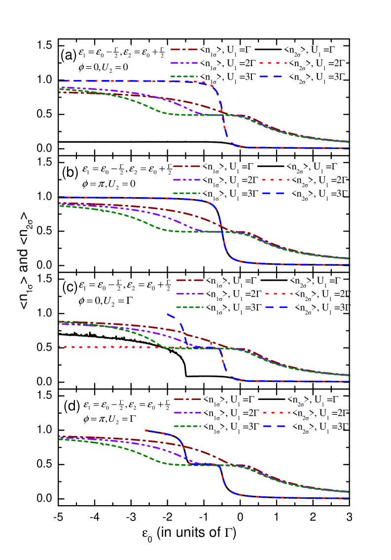
Figure 5: The spectra of Coulomb-modified average electron occupation numbers in QD-1 and QD-2. The relevant parameters are the same as those in Fig.4.

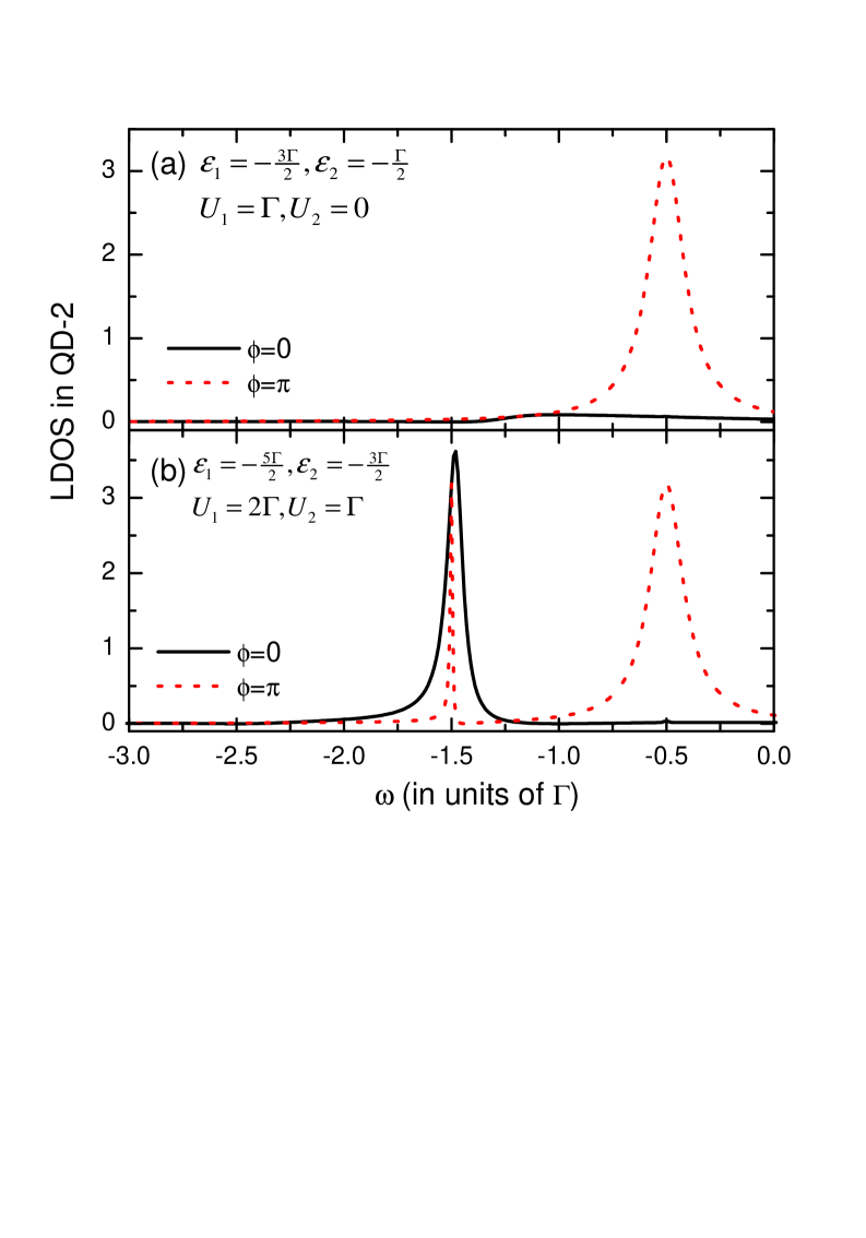
Figure 6: The spectra of LDOS in QD-2. The values of the relevant parameters are assumed to be $\varepsilon_{1}=-\frac{3}{2}\Gamma$, $\varepsilon_{2}=-\frac{1}{2}\Gamma$, $U_{1}=\Gamma$, and $U_{2}=0$ in (a); $\varepsilon_{1}=-\frac{5}{2}\Gamma$, $\varepsilon_{2}=-\frac{3}{2}\Gamma$, $U_{1}=2\Gamma$, and $U_{2}=\Gamma$ in (b).

References

- (1) U. Fano, Phys. Rev. 124, 1866 (1961).
- (2) A. E. Miroshnichenko, S. Flach, and Y. S. Kivshar, cond-mat/arXiv:0902.3014.
- (3) R. K. Adair, C. K. Bockelman, and R. E. Peterson, Phys. Rev. 76, 308 (1949).
- (4) U. Fano and A. R. P. Rau, Atomic Collisions and Spectra ( Academic, Orlando, 1986 ).
- (5) F. Cerdeira, T. A. Fjeldly, and M. Cardona, Phys. Rev. B 8, 4734 (1973).
- (6) J. Faist, F. Capasso, C. Sirtori, K. W. West, and L. N. Pfeiffer, Nature (London) 390, 589 (1997); H. Schmidt, K. L. Campman, A. C. Gossard, and A. Imamoglu, Appl. Phys. Lett. 70, 3455 (1997).
- (7) V. Madhavan, W. Chen, T. Jamneala, M. Crommie, and S. Wingreen, Science 280, 567 (1998).
- (8) S. Rotter, F. Libisch, J. Burgdöfer, U. Kuhl, and H.-J. Stökmann, Phys. Rev. E 69, 046208 (2004).
- (9) J. Göres, D. Goldhaber-Gordon, S. Heemeyer, and M. A. Kastner, Phys. Rev. B 62, 2188 (2000).
- (10) I. G. Zacharia, D. Goldhaber-Gordon, G. Granger, M. A. Kastner, Y. B. Khavin, H. Shtrikman, D. Mahalu, and U. Meirav, Phys. Rev. B 64, 155311 (2001).
- (11) K. Kobayashi, H. Aikawa, S. Katsumoto, and Y. Iye, Phys. Rev. Lett. 88, 256806 (2002); Phys. Rev. B 68, 235304 (2003); M. Sato, H. Aikawa, K. Kobayashi, S. Katsumoto, and Y. Iye, Phys. Rev. Lett. 95, 066801 (2005); K. Kobayashi, H. Aikawa, A. Sano, S. Katsumoto, and Y. Iye, Phys. Rev. B 70, 035319 (2004).
- (12) X. R. Wang, Yupeng Wang, and Z. Z. Sun, Phys. Rev. B 65, 193402 (2002).
- (13) M. E. Torio, K. Hallberg, S. Flach, A. E. Miroshnichenko, and M. Titov, Eur. Phy. J. B 37, 399-403 (2004).
- (14) A. C. Johnson, C. M. Marcus, M. P. Hanson, and A. C. Gossard, Phys. Rev. Lett. 93, 106803 (2004).
- (15) A. Fuhrer, P. Brusheim, T. Ihn, M. Sigrist, K. Ensslin, W. Wegscheider, and M. Bichler, Phys. Rev. B 73, 205326 (2006).
- (16) A. W. BlickHolleitner, C. R. Decker, H. Qin, K. Eberl, and R. H. Blick, Phys. Rev. Lett. 87 256802 (2001); A. W. Holleitner, R. H. Blick, A. K. Hüttel, K. Eberl, and J. P. Kotthaus, Science 297 70 (2002); A. W. Holleitner, R. H. Blick, and K. Eberl Appl. Phys. Lett. 82 1887 (2003).
- (17) J. C. Chen, A. M. Chang, and M. R. Melloch Phys. Rev. Lett. 92 176801 (2004).
- (18) J. L. D’Amato, H. M. Pastawski, and J. F. Weisz, Phys. Rev. B 39, 3554 (1989).
- (19) E. Tekman and P. F. Bagwell, Phys. Rev. B 48, 2553 (1993); J. U. Nökel, and A. D. Stone, Phys. Rev. B 50, 17415 (1994).
- (20) B. R. Bułka and P. Stefański, Phys. Rev. Lett. 86, 5128 (2001).
- (21) W. Hofstetter, J. König, and H. Schoeller, Phys. Rev. Lett. 87, 156803 (2001).
- (22) B. Kubala and J. König, Phys. Rev. B 65, 245301 (2002).
- (23) A. Sila, Y. Oreg, and Y. Gefen, Phys. Rev. B 65, 195316 (2002).
- (24) K. Kang and S. Y. Cho, J. Phys.: Condens. Matter 16, 117 (2004).
- (25) Z.-M. Bai, M.-F. Yang, and Y.-C. Chen, J. Phys.: Condens. Matter 16, 4303 (2004).
- (26) H. Lu, R. Lü, and B. F. Zhu, Phys. Rev. B 71, 235320 (2005).
- (27) M. L. Ladron de Guevara, F. Claro, and P. A. Orellana, Phys. Rev. B 67, 195335 (2003).
- (28) G. H. Ding, C. K. Kim, and K. Nahm, Phys. Rev. B 71, 205313 (2005).
- (29) C. Karrasch, T. Enss, and V. Meden, Phys. Rev. B 73, 235337 (2006).
- (30) H. Lu, R. Lü, and B. F. Zhu, J. Phys.:Condens. Matt. 18, 8961 (2006).
- (31) W. Gong and C. Jiang, J. Appl. Phys. 106, 013710 (2009).
- (32) A. A. Clerk, X. Waintal, and P. W. Brouwer, Phys. Rev. Lett. 86, 4636 (2001).
- (33) F. Chi and S. S. Li, J. Appl. Phys. 100, 113703 (2006).
- (34) L. G. G. V. D. da Silva, N. Sandler, P. Simon, K. Ingersent, and S. E. Ulloa, Phys. Rev. Lett. 102, 166806 (2009).
- (35) S. Datta, (Cambridge University Press, Cambridge, England, 1997).
- (36) Y. Meir and N. S. Wingreen, Phys. Rev. Lett. 68, 2512 (1992); A. P. Jauho, N. S. Wingreen, and Y. Meir, Phys. Rev. B 50, 5528 (1994).
- (37) W. Gong, Y. Zheng, Y. Liu, and T. Lü, Phys. Rev. B 73, 245329 (2006) and the references therein.
- (38) Y. Liu, Y. Zheng, W. Gong, and T. Lü, Phys. Lett. A 365, 495 (2007).
- (39) W. Gong, Y. Zheng, Y. Liu, and T. Lü, Physica E 40, 618 (2008).
- (40) Y. Qi, J.-X. Zhu, S. Zhang, and C. S. Ting, Phys. Rev. B 78, 045305 (2008).
- (41) M. Zaffalon, Aveek Bid, M. Heiblum, D. Mahalu, and V. Umansky, Phys. Rev. Lett. 100, 226601 (2008).
- (42) R. Bulla, T. A. Costi, and T. Pruschke, Rev. Mod. Phys. 80, 395 (2008); H. Schoeller and F. Reininghaus, Phys. Rev. B 80, 045117 (2009).
- (43) M. Sindel, A. Sila, Y. Oreg, and J. Delft, Phys. Rev. B 72, 125316 (2005).
- (44) V. Meden, and F. Marquardt, Phys. Rev. Lett. 96, 146801 (2006).