Succinct Representation of Well-Spaced Point Clouds

Abstract

A set of $n$ points in low dimensions takes $\Theta(nw)$ bits to store on a $w$-bit machine. Surface reconstruction and mesh refinement impose a requirement on the distribution of the points they process. I show how to use this assumption to lossily compress a set of $n$ input points into a representation that takes only $O(n)$ bits, independent of the word size. The loss can keep inter-point distances to within 10% relative error while still achieving a factor of three space savings. The representation allows standard quadtree operations, along with computing the restricted Voronoi cell of a point, in time $O(w^{2}+\log n)$, which can be improved to time $O(\log n)$ if $w\in\Theta(\log n)$. Thus one can use this compressed representation to perform mesh refinement or surface reconstruction in $O(n)$ bits with only a logarithmic slowdown.

1 Introduction

My goal in this paper is to produce a succinct point location structure to support surface reconstruction and mesh refinement tasks while using asymptotically less space than the current state of the art. To this end, I present a compressed data structure that provides an interface much like that of a $2^{d}$-tree (for readability I call this a quadtree). Funke and Milosavljevic [FM07] show how to use an quadtree so that given a sufficiently dense set of points in 3-space that lie on an unknown 2-manifold, we can reconstruct a triangulation that approximates the 2-manifold, in time $O(n\log n)$. Hudson and Türkoğlu [HT08] show how to use a quadtree to augment an arbitrary set of points in $d$ dimensions and generate a well-spaced point set, that is, one whose Delaunay triangulation will produce a good mesh for scientific applications, usually in $O(n\log n)$ time (more precisely, in $O(n\log\Delta)$ time where $\Delta$ is the geometric spread). As a special case, if the point set is well-spaced, they compute the Voronoi cell of an arbitrary point in constant time.

The storage used by the two algorithms is in two parts: the quadtree, and the point coordinates. A balanced quadtree [BEG94] over $n$ arbitrary points can have a superlinear number of quadtree cells. However, the requirements of the tasks at hands impose limits on the size of the quadtree. In the surface reconstruction case, the $n$ points of the input must be locally regular (which has various definitions, see Section 2). In the mesh refinement case, the output must be well-spaced, and I use $n$ to refer to the number of points in the output. These requirements imply that the quadtree only has $O(n)$ leaves and internal nodes [HMPS09]. Thus, in a cell probe model of computation with real arithmetic, the storage is linear. Sadly, this is a completely fictional machine. In the more realistic word RAM model, each pointer must be at least $\log(n)$ bits long for each point to have a distinct memory address, whereas each coordinate must be at least $\log(n^{1/d})$ bits for each point to have a distinct location in space. For simplicity I assume both coordinates and pointers have the same length, namely $w$ bits.

The first part of this paper (Sections 2–4) lays the groundwork, showing that we can use a small interface on top of a quadtree in order to support the richer operations that Funke et al or Hudson et al require. I show how to implicitly represent the balanced quadtree by sorting the coordinates in Morton order [Mor66] (also known as the Z-order), a trick that extends the so-called framework of Bern, Eppstein, and Teng [BET99]. This all but eliminates the storage cost of the quadtree, while only requiring a logarithmic slowdown.

The second and more interesting part of the paper (Sections 5–7) deals with compressing the geometric storage requirements at asymptotically no greater runtime cost. The intuition is that, given that we have the points in sorted order, the distance between one point and the next is generally small, therefore the difference in coordinates is small. What my structure stores for each vertex is the coordinates of each point, rounded to be at a fixed position in its quadtree leaf square: the representation is lossy, as it must be (Lemma 6.1). It keeps track of the number of bits that were rounded off by storing the quadtree leaf size. Intuitively, the leaf sizes generally do not change much from one point to the next, so it only stores the difference in the leaf sizes. Intuitively, only the low bits of the coordinates of each point change from one point to the next in the sorted order, so it only stores the XOR of the coordinates. To prove these intuitions I show a correspondence between the storage requirements and a depth-first traversal of the balanced quadtree: since we can traverse an $n$-node tree by visiting each node only once, we can store the $n$ geometric points in $O(n)$ bits. I discuss very preliminary experimental results in the conclusions.

Traditional compression techniques read in the entire input into memory and compress it, the intent being to then transmit the file over the network, or to save on disk storage. But the entire point of my work here is to handle inputs that are too big for main memory, without switching to an out-of-core or streaming framework. I show instead how to read points in from a file, without exceeding the space bounds, using $w$ scans through the file for a total of about $O(n\log^{2}n)$ time to initialize the structure assuming words of length about $\log n$.

Prior work:

Traditional work on mesh compression store both the mesh topology and the mesh geometry using a 10–20 bits per vertex, most of it geometric information [PKK05, survey]. Unfortunately, this is inapplicable since in the setting of this paper, we do not have connectivity information: in the reconstruction case, connectivity is the final goal, and in the refinement case, connectivity is too expensive to maintain.

Another related approach is a succinct mesh structure by Blandford et al [BBCK05, Bla05], which can be used to compute the Delaunay triangulation of a set of points. They compress the connectivity as they discover it, but do not compress the geometry. Thus our approaches are complementary: I show how to compress the geometry, but not the connectivity. It remains future work to see how precisely to meld the two ideas.

2 Preliminaries

Machine Model:

I assume we operate on the $w$-bit word RAM. That is, pointers are $w$-bit memory addresses, and coordinates consume $w$ bits also. For simplicity, I assume the points are at positive fixed-point (i.e. integer) coordinates; it will be clear that the sign bit and exponent of floating point notation can easily be handled. Coordinates thus go from 0 to $W\equiv 2^{w}-1$.

Input Assumption:

Given a point set $P$ and subspace $S$, the restricted Voronoi diagram assigns to each $p\in P$ a cell $V_{p}$ consisting of the set of points $x\in S$ that are closer to $p$ than to any other point $q\in P$. In other words, it is the intersection of the Voronoi diagram of $P$ and the subspace $S$. The restricted Delaunay neighbours of $p\in P$ are the points of $Q$ whose restricted Voronoi cells intersect $V_{p}$. The results herein assume the restricted Voronoi cells are well-spaced in the following sense:

Definition 2.1

The aspect ratio of $V_{p}$ (and, by extension, of $p$) is the ratio $\frac{\max_{x\in V_{p}}|px|}{\min_{q\in P}|pq|}$. We say that $P$ is $\rho$-well-spaced if for all $p\in P$, the aspect ratio of $V_{p}$ is at most $\rho$.

In the mesh refinement problem, one of the goals is precisely to generate a well-spaced set of points. In surface reconstruction, there are many assumptions that can be required of the input. In particular, many algorithms are only guaranteed to work if the input is an $\epsilon$-net in the following sense:

Definition 2.2

Let $f:S\to\mathbb{R}$ be a Lipschitz function; that is, $f(x)\leq f(y)+|xy|$ for any $x$ and $y$ both in $S$. Then the $n$-point set $P\subset S$ is an $\epsilon$-net over $S$ if:

• for all $x\in S$, there is a point $p\in P$ such that $|px|\leq\epsilon f(x)$

• for all $p\in P$, for all $q\in P\backslash\{p\}$, $|pq|\geq f(p)$.

An $\epsilon$-net is well-spaced. Consider a restricted Voronoi cell $V_{p}$. The denominator in the aspect ratio is at least $f(p)$ by definition. For the numerator, consider a point $x\in V_{p}$. We know that $|px|\leq\epsilon f(x)$. By the Lipschitz assumption on $f$, we know $f(x)\leq f(p)+|px|$. Thus $|px|\leq f(p)/(1-\epsilon)$. In other words, the aspect ratio is at most $\epsilon/(1-\epsilon)$.

3 Quadtree Query Structure

The query structure provides an interface that the balanced quadtree [BEG94] can support. See Figure 1.

$\textsc{SquareOf}(p)$	Return the leaf that contains the point $p$
$\textsc{Vertices}(s)$	Return a pointer to the set of vertices in the square $s$
$\textsc{Neighbour}(s,i)$	Return the $i$th equal-sized neighbour of the square $s$
$\textsc{Child}(s,i)$	Return the $i$th child of the square $s$
$\textsc{Voronoi}(p)$	Compute the restricted Voronoi cell of $p$

Figure 1: Interface I support for the quadtree. Voronoi is implemented in terms of the first four queries. All run in constant time for a pointer-based quadtree.

In my parlance, a quadtree is a tree structure defined recursively: each node, which I call a square, has a size and a defining point, namely its minimum corner. Internal squares have exactly $2^{d}$ children. Leaf squares store a list of the points they contain. We can recursively define the balanced quadtree of Bern, Eppstein, and Gilbert [BEG94]: we start with the root square, with minimum corner at the origin and size $W$. We split the largest quadtree leaf square that is either crowded or unbalanced. A square is crowded if either it contains two or more vertices, or it contains exactly one vertex, and a neighbouring square contains one or more vertices. A square is unbalanced if there is a neighbouring square of one quarter the size. Splits are in the middle of the node: the children are non-overlapping and have half the size of their parent. The main obvious property we need here is that, in the balanced quadtree, each vertex is assigned to exactly one leaf square, and all the equally-sized neighbouring squares are empty of any vertices.

The traditional representation has each square storing $2^{d}$ pointers to children, $3^{d}-1$ pointers to neighbouring equal-sized squares, the coordinates, and the height (the logarithm of the size) of the square. Leaf squares store a pointer to the set of vertices they contain. Each point stores a pointer to the square in which it lies. The implementations of most of the functions are fairly obvious given this representation. Insertion and deletion are also relatively straightforward. They take time linear in the depth of the tree; given that the points are at integer coordinates, the depth of the tree is at most $w$. I should draw attention to the fact that Vertices is not required to report a copy of the set of vertices in the square, but merely pointers that can be used to iterate over the set.

The restricted Voronoi query requires a bit more discussion. If the subspace to which we are restricting is the entire volume $[0,W]^{d}$, Hudson and Türkoğlu [HT08, Theorem 7] showed how to compute the restricted Voronoi cell of a point assuming the point set is well-spaced: First, look up the square that contains the query point $q$. Then, scan the squares, in order of distance from $q$. Vertices encountered during the scan are stored as the putative Voronoi neighbours. Using the appropriate notion of distance, this procedure indeed computes the exact Voronoi cell, and only accesses a bounded number of squares.

For an unknown 2-manifold $S$ lying in arbitrary dimension, assuming a locally regular sample (which is a more stringent requirement than the $\epsilon$-net condition) we can use the procedure defined by Funke and Milosavljevic [FM07] to compute in constant time (looking up a bounded number of squares) the Voronoi cell restricted to a 2-manifold $S^{\prime}$ that approximates $S$. For higher-dimensional manifolds, the situation is still open, though we know how to compute a bounded-size superset of the restricted Voronoi cell [Hud08] that still needs to be pruned [CDR05]. Nevertheless, in all cases, the Voronoi query is in two parts: (a) look up the balanced quadtree square $s$ that contains the query point. (b) look up a bounded number of nearby quadtree squares, each of them no more than a constant factor smaller than $s$.

4 Implicit Quadtree via Morton Ordering

The first new result in this paper is to show how to nearly eliminate the cost of storing the quadtree. The key observation is that the balanced quadtree is formed from the leaves of a trie with arity $2^{d}$. To recur into a split child is equivalent to reading one more bit of each coordinate. A trie square $s$ is represented by its minimum corner $p$ and a height $h$. It must be that $p$ is a prefix of length $d(w-\log h)$, and the lower $\log h$ bits of each coordinate are all zero; otherwise, $s$ is not a square of the trie. To split a trie square, simply halve $h$ and use one additional bit of each coordinate in $p$. To find a neighbour of a trie square, add $h$ to the appropriate coordinates of $p$.

This motivates computing the Morton Order [Mor66] (also known as the Z-order). Define the Morton number of a point as the $(d\log n)$-width integer formed by interleaving the bits of the coordinates, see Figure 2. The Morton order of a set $P$ sorts by the Morton number. The data structure representing the quadtree is then simply an array: we explicitly store the coordinates of the points. I now show how to implement the quadtree interface of the prior section:

Decimal:	(3, 5)		(4, 2)
Binary:	(011, 101)		(100, 010)
Morton:	01 10 11	$<$	10 01 00

Figure 2: The Morton order of points (3, 5) and (4, 2).

$\textsc{Vertices}(s)$:

We can look up the contents of a trie square $s=(p,h)$: search for the successor of the minimum corner of $s$ (namely, $p$) in the Morton order, and search for the predecessor of the maximum corner of $s$ (namely, $p$ translated by $h$ in each coordinate). Every point strictly within this range has a prefix that places it within the square of interest. The two binary searches take $O(\log n)$ time each and return the bounds of a subarray over which we can iterate.

Neighbour and Child:

The representation of a square now is merely a prefix and a size, which allows computing these functions in constant time using mere arithmetic. To get an equal-sized neighbour of the square, merely add or subtract the size from each coordinate. To get the child of a square, append $d$ bits to the prefix and halve the size.

$\textsc{SquareOf}(p)$:

The leaf square that contains $p$ and is uncrowded shares a common prefix with $p$; the only question is how much of the prefix needs to be kept. The answer can be determined by binary search over the $w$ possible answers. Given a trie square $s$, we test whether the square is crowded. First, do a range search for $s$. If it indicates a range of two or more vertices, then $s$ is crowded. If it indicates an empty range, $s$ is uncrowded. Otherwise, if the range of $s$ contains exactly one vertex, iterate over each neighbour $s^{\prime}$ of $s$ and do a range search on $s^{\prime}$. If $s^{\prime}$ is non-empty, $s$ is crowded, otherwise is it uncrowded. There are $3^{d}-1$ neighbours of $s$, so testing for crowding takes $O(\log n)$ time. We do this $O(\log w)$ times, for a total of $O(\log(n)\log(w))$ runtime.

Theorem 4.1

Given a well-spaced point set $P$ in an array sorted by Morton order, we can compute the restricted Voronoi cell of a given vertex $v$ in $O(\log(n)\log(w))$ time.

5 Lossless Compression

Given a list of integers $i_{1},\ldots,i_{n}$, we can often reduce the storage requirement of the set (normally $wn$ bits) by difference-encoding the integers, assuming subsequent integers are on average close. The storage representation is as follows: let $\delta_{j}\equiv i_{j}-i_{j-1}$. We store the first element $i_{1}$ in longhand, using $w$ bits. For the $j$th element, we store only $\delta_{j}$ using a variable bit length encoding of $\delta_{j}$. For concreteness, I assume we use a gamma-code: first, a count in unary (using zeroes) of the number of bits needed to represent $\delta_{j}$, then $\delta_{j}$ starting at its leading ’1’ bit, and finally a sign bit (not necessary if $\delta_{j}$ is zero). The gamma code uses 1 bit if $\delta_{j}=0$, or $1+2(\lg|\delta_{j}|+1)$ for non-zero values. Thus, if on average $\delta_{j}$ is $O(1)$, the set takes only $w+O(n)$ bits to store. Note that instead of using the subtraction operator, we could have used the bitwise operator XOR and achieved the same asymptotic result. I refer to this encoding strategy as the difference-code when using the subtraction operator, and the xor-code when using bitwise exclusive or.

value	uncompressed	bits	xor	xor-coded	bits
$(5,2)$	00101,00010	10		00101,00010	10
$(6,3)$	00110,00011	10	(11, 1)	0011,01	6
$(8,4)$	01000,00100	10	(1110, 111)	00001110,000111	14
$(9,6)$	01001,00110	10	(1, 10)	01,0010	6
$(10,6)$	01010,00110	10	(11, 0)	0011, 1	5
total		50			41

Figure 3: The encoding of a list of 5 points on a 5-bit machine. On a 32-bit machine the encodings would take 320 and 95 bits respectively.

My encoding strategy applies the xor-code to each dimension in turn. That is, first, sort the points by Morton order. Second, xor-code the array consisting of all their $x$ coordinates. Third, xor-code their $y$ coordinates, and so on. See Figure 3. I use the xor-code rather than the difference-code for an easier analysis; it happens to also be very slightly more space-efficient in practice.

Theorem 5.1

Let $f$ be a constant function defined on a compact space $S$; that is, there is a constant $f_{0}$ such that $f(x)=f_{0}$ for all $x\in S$. Let $P$ be a set of $n$ points that forms an $\epsilon$-net over $S$ with respect to $f$, for some constant $\epsilon$. Then we can store $P$ using $O(w+n)$ bits, where the constant depends only on $f_{0}$, $\epsilon$, and the dimension $d$.

Proof:   The proof is via an equivalence to the quadtree. Consider the full trie—all squares representable with $d$ integers of $w$ bits each. A point $p$ denotes a path from root to leaf in this trie. The representation of the difference between $p_{i-1}$ and $p_{i}$ denotes a path from the first point to the second. For simplicity, assume all the coordinates have equal-length XORs (if not, we store only less than is analyzed here). A 0 bit of the length field in each of the $d$ xor-encoded dimensions corresponds to moving up one level in the quadtree. A bit in the xor in each of the $d$ dimensions corresponds to choosing a child into which to travel. Thus the total number of bits of the encoding of the difference between $p_{i-1}$ and $p_{i}$ is precisely $d$ times the length of the path.

The Morton order is a depth-first ordering of the points (the non-empty leaves); therefore, the overall path length of traversing the points in Morton order is linear in the number of nodes of the trie (internal or leaf) that contain at least one point. I divide this set of nodes in two: first, non-empty nodes not in the balanced quadtree over $P$; second, non-empty nodes that are indeed in the balanced quadtree. We know by the $\epsilon$-net condition that there is a point within distance $2\epsilon f_{0}$ of $p$, so $s_{p}$ has size at most $\epsilon f_{0}$ or else the cell is crowded (which would contradict that it is a leaf). Thus the first category contains at most $\lg(2\epsilon f_{0})n=O(n)$ nodes. To count the second category, consider the smallest quadtree cell $s_{S}$ that contains all of $S$. A theorem of Hudson, Miller, Phillips, and Sheehy shows that within $s_{S}$, a volume mesh such as the balanced quadtree over the $(1-\epsilon)^{-1}$-well-spaced set $P$ has $O(n)$ leaves [HMPS09]. The number of nodes in a $2^{d}$-tree is only a constant fraction larger than the number of leaves. We are still left with counting the ancestors of $s_{S}$; there are at most $w$ of them.

Putting the arguments together, we see that the compressed representation takes precisely $dw$ bits to store the first point, plus $O(n+w)$ bits to store the subsequent points, assuming $f_{0}$, $\epsilon$, and the dimension $d$ are constants.   

6 Lossy Compression

The lossless compression of the previous section only provably works if the points are on average at a distance near unity from their predecessor. While many data sets have this behaviour (for example, the Stanford bunny data set, scaled by $10^{7}$), so far our technique does not handle well-spaced point sets as advertised. For example, in one dimension, the points $1,2,\ldots,2^{n}$ are well-spaced but will require $n\log n$ bits in the lossless compression format. This motivates developing what amounts to a compressed floating-point format.

More devastatingly, we can develop an information-theoretic lower bound on our ability to compress data. The adversary can take an arbitrary well-spaced subset in $w/2$ bits, then append a ’0’ to each integer followed by $w/2-1$ bits of random noise. This noised set is only slightly less well-spaced than the original: the ’0’ keeps vertices from becoming arbitrarily close to each other. Information theoretic arguments show that with high probability, the adversary has won: no code can store $o(w)$ bits and represent the random noise exactly. The lower bound here does not disprove the claim of Theorem 5.1: $f_{0}$ is $2^{w/2}$, which is not a constant factor. This means we are forced to round the input.

Lemma 6.1

No data structure can exactly store an arbitrary well-spaced set of $n$ points in $[0,W]^{d}$ using $o(nw)$ bits.

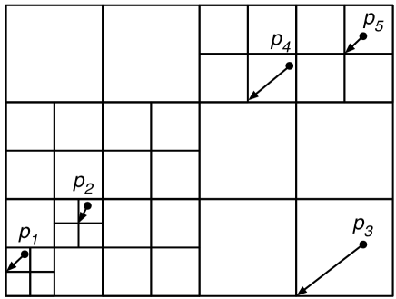
Figure 4: Balanced quadtree of five points in Morton order. Each point has an arrow showing its rounded form when $\gamma=0$.

Rounding:

The rounding routine takes a parameter $\gamma$, which corresponds to the desired precision: greater $\gamma$ is less lossy, but requires storing more information. Consider a point $p$ whose balanced quadtree leaf is at height $h$. To round, zero out the lower $h-\gamma$ bits of each coordinate of $p$, producing a point $p^{\prime}$. Intuitively it should be clear that with sufficiently large $\gamma$, we can maintain any desired well-spacing or $\epsilon$-net property, so that rounding has little effect. The key notion is that the balanced quadtree over the rounded set $P^{\prime}$ is identical to the balanced quadtree over the original set $P$. See Figure 4.

Lemma 6.2

Given a pair of input points $p$ and $q$, after rounding them to $p^{\prime}$ and $q^{\prime}$, both the ratio $|p^{\prime}q^{\prime}|/|pq|$ and its reciprocal are bounded by $1+2^{1-\gamma}\sqrt{d}$.

Proof:   By the triangle inequality, $|p^{\prime}q^{\prime}|\leq|pq|+|pp^{\prime}|+|qq^{\prime}|$. Without loss of generality, assume $p$ lies in the larger quadtree leaf, and that this leaf has size $s$. Rounding moves the points by at most $2^{-\gamma}\sqrt{d}s$. Thus $|p^{\prime}q^{\prime}|\leq|pq|+2^{1-\gamma}\sqrt{d}s$. Finally, the definition of crowding implies that $s\leq|pq|$, which proves $|p^{\prime}q^{\prime}|\leq(1+2^{1-\gamma}\sqrt{d})|pq|$. The proof for the reciprocal is symmetric.   

Encoding:

Since we have rounded off some bits, it would be wasteful now to represent all the zeroes. Instead, we will store only the number of bits we rounded off — that is, the height $h$. Note that this means we are essentially storing a floating-point number. Furthermore, from one point to the next, the height differs only slightly, so I recommend to difference-code the heights. Thus, assuming $\gamma=0$, the two-dimensional point $(x_{i},y_{i})$ whose balanced quadtree leaf is at height $h_{i}$ is represented as the triple of integers $(h_{i}-h_{i-1},(x_{i}\mathop{\textbf{xor}}x_{i-1})>>h_{i},(y_{i}\mathop{\textbf{xor}}y_{i-1})>>h_{i})$ where $>>$ denotes a logical right shift.

To decode a point $\mathbf{x}_{i}$ knowing $\mathbf{x}_{i-1}$ and $h_{i-1}$, we decode $\partial h_{i}$ and add $h_{i-1}$ to obtain $h_{i}$. Then we decode each $\delta\mathbf{x}_{i,j}$ in turn, shift $\mathbf{x}_{i-1,j}$ right by $h_{i}-\gamma$ bits, xor with $\delta\mathbf{x}_{i,j}$, then shift this quantity left by $h_{i}-\gamma$.

Theorem 6.3

Let $P$ be a set of $n$ $\rho$-well-spaced points. Round $P$ to $P^{\prime}$ with the rounding coefficient $\gamma$. We can store $P$ using $O(w+n\gamma)$ bits, where the constant depends only on $\rho$ and the dimension $d$.

Proof:   As in the prior theorem, we use the correspondence with the quadtree. The bits we store for the coordinates are paid for by the depth first search argument as before, except for the $\gamma$ bits we store for additional precision. It remains to count the difference-encoded bits for the height.

Consider the following string we could compute during a depth first traversal through the balanced quadtree: store a $+$ when the search heads to a parent, and a $-$ when it moves to a child. The total number of symbols thus stored is bounded by the number of nodes of the quadtree, which is $O(n)$ for a well-spaced set of points. I claim the height differences are essentially a summary of this same information: indeed, the height difference between $p_{i}$ and $p_{i+1}$ is the number of $+$ symbols seen when moving from the quadtree leaf that contains $p_{i}$ to the least common ancestor with $p_{i+1}$, minus the number of $-$ symbols from the least common ancestor to the leaf that contains $p_{i+1}$. This is clearly more parsimonious (or at worst no worse) than run-length-encoding the string of $+$ and $-$ symbols. In the worst case, run-length-encoding takes $O(n)$ bits when the lengths are stored using the gamma code.   

7 Fast Queries

The structure we have discussed so far takes only $O(n+w)$ bits to store $n$ well-spaced points, as promised, but it does not fulfill the promise of on-line queries in sublinear time. In this section I show how to add a standard (that is, uncompressed) balanced binary tree over the structure to achieve the faster runtime.

Recall that a binary search tree over $N$ elements requires $O(N)$ pointers, which is $O(Nw)$ bits. This means we can store as many as $n/w$ elements in the tree and still only use $O(n)$ bits. The solution, then, is to break the encoded array of well-spaced points into subarrays of size $n/w$. In sum, encoded, the array took $O(n+w)$ bits. Broken up, we need to pay $O(w)$ bits to encode the first point in each subarray in longhand (which forms the key in the search tree). There are $O(n/w)$ subarrays, so this overhead amounts to $O(n)$, or a total of $O(n+w)$ bits for the entire array, the overhead for breaking it into subarrays, and the binary tree.

A Vertices query in our structure takes time $O(\log(n/w))\subset O(\log n)$ time to find the correct subarray. Then it must perform a linear scan in the subarray. The number of points in the subarray is $O(w)$. While on average each point requires $O(1)$ bits, in the worst case, they can each take $O(w)$ bits, so the subarray may have size $O(w^{2})$ bits. Naively, this will take $O(w^{2})$ time to decompress. With tables of size $\Theta(n)$ bits, we can decompress $\Theta(\log n)$ bits at a time, thereby decompressing in $O(w^{2}/\log n)$ time. If $w\in\Theta(\log n)$, we decompress in $O(w)=O(\log n)$ time.

A SquareOf query from an uncompressed array in Morton order required $O(\log w)$ Vertices queries. Now, however, there are two cases. In the losslessly compressed structure, the square size is always small: we need only try $O(\log f_{0})$ Vertices queries before we find the quadtree size. In the lossily compressed structure, we explicitly store the square size, which means we can reproduce the quadtree square of a point simply by searching for the point itself.

$\textsc{SquareOf}(p)$	$O((w^{2}/\log n)+\log n)$
$\textsc{Vertices}(s)$	$O((w^{2}/\log n)+\log n)$
$\textsc{Neighbour}(s,i)$	$O(1)$
$\textsc{Child}(s,i)$	$O(1)$
$\textsc{Voronoi}(p)$	$O((w^{2}/\log n)+\log n)$

Figure 5: Runtimes for the compressed structure.

Theorem 7.1

After preprocessing, we can store a well-spaced set of points using $O(n)$ bits while supporting the quadtree operations in the times listed in Figure 5.

8 Dynamic Operation

So far we have not discussed the construction of our structures. Inserting a vertex requires a semi-dynamic compression format. The structure of the prior section is a balanced tree with fat leaves storing subarrays of $\Theta(w)$ vertices. To support insertions, we let the size of the subarrays vary between $w$ and $2w$. Upon adding a vertex $v$, we find the appropriate subarray and add $v$ to it in the appropriate spot, encoding it and re-encoding its successor. If $v$ becomes the head of the subarray, we update the dictionary appropriately. Finally, if the new subarray is too large, we split it in two equal halves.

Lemma 8.1

We can insert a vertex into our compressed structure in time $O(w+\log n)$.

0:  

1:  open the file

2:  let $n$ be the number of points in the file

3:  let $P$ to the compressed set of $n$ points all at the origin with height $w$

4:  let $B$ to be a length $n$ vector of $\log\gamma$-bit integers with initial value 0

5:  for $i=w-1$ down to $0$ do

6:     reopen the file

7:     $P^{\prime}\leftarrow\emptyset$

8:     for point $j=1$ to $n$ do

9:        if $B[j]$ is $\gamma$ then

10:           copy the $j$th point of $P$ to $P^{\prime}$

11:        else

12:           Read $p_{j}$ from the file.

13:           $p^{\prime}_{j}\leftarrow$ zero out the $i$ least significant bits of $p_{j}$

14:           add $p^{\prime}_{j}$ with height $w$ to $P^{\prime}$

15:     for point $j=1$ to $n$ do

16:        Read the point $p^{\prime}_{j}$ and height $h^{\prime}_{j}$ from $P^{\prime}$

17:        Check if one of the neighbours of the square $(p^{\prime}_{j},h^{\prime}_{j})$ contains a point

18:        If not, increment $B[j]$ to maximum value $\gamma$. $P\leftarrow P^{\prime}$

19:  return $P$

Figure 6: Initializing the compressed point set in $w$ scans of an input file.

This assumes the input was already rounded (or that we are not rounding). Efficiently rounding is a difficult problem: we need to know the balanced quadtree cell that contains a point $p$ to know how much information to discard. But we can’t know that until we have read the entire file into memory, which takes too much space. The solution to this problem is to scan the input file repeatedly. In the first scan, we read only the first (most significant) bit of each coordinate. Having read the file once, if we now have enough information to compute the balanced quadtree leaf of any point, we no longer need to read any more bits of that point, but we still need to read more bits of the other points. Therefore, we mark the points either as balanced or not using a bitvector $B$. In each subsequent scan, we simply copy the points that we know sufficiently well, while we read an additional bit of the points we still need to refine. In the algorithm of Figure 6, $B$ is widened to count up to $\gamma$ to allow for less aggressive rounding. Obviously, in practice, one would want to read multiple bits at a time, to reduce the number of scans.

Theorem 8.2

We can construct a compressed query structure in $w$ scans of the input file, in time $O(nw(\log(n)+w^{2}/\log n))$, never using more than $O(n)$ bits of memory. For $w=\Theta(\log n)$ this is $O(n\log^{2}n)$ time.

Proof:   Each scan takes linear time to read the file, then performs $O(1)$ Vertices queries per vertex read, each of which has the ugly runtime presented in the prior section. Encoding, to add the new point to $P^{\prime}$, has equal runtime.   

Given the spatial locality between the queries, it seems likely that one could improve upon this using finger searching data structures and caching the decompression. An alternate improvement would be to amortize the $w^{2}$-bit worst-case subarray decompression time by the fact that we only have a total of $O(n)$ bits. I conjecture it should be possible to use only $O(nw)$ time over $w$ scans without violating the space bound.

9 Compressed Mesh Refinement

The previous sections assumed the mesh was given as a well-spaced set of points. But where did this data come from, if it doesn’t fit in memory? Here I show how to construct a well-spaced superset (i.e., a quality mesh) of an ill-spaced input by adding a minimal number of Steiner points [BEG94, Rup95]. I show that the Steiner points are asymptotically free to store, and that we can compute them using just the queries for our compressed quadtree.

0:  

1:  $r\leftarrow 0$

2:  $M\leftarrow P$

3:  while $r$ finite do

4:     $r^{\prime}\leftarrow\infty$

5:     for $v\in M$ do

6:        $s_{v}\leftarrow\textsc{SquareOf}(v)$

7:        if $|s_{v}|>r$ then

8:           $r^{\prime}\leftarrow\min(r^{\prime},|s_{v}|)$

9:        else

10:           compute $2\rho$-clipped Voronoi of $v$

11:           while aspect ratio of $v$ exceeds $\rho$ do

12:              $r^{\prime}\leftarrow r$

13:              choose $x\in$ clipped Voronoi with $|vx|\geq\rho\mathrm{NN}(v)$

14:              round $x$ as for geometry compression

15:              insert $x$ into $M$

16:              recompute $2\rho$-clipped Voronoi of $v$

17:     $r\leftarrow r^{\prime}$

Figure 7: Mesh refinement using a compressed mesh.

At heart, the algorithm I propose iterates over each vertex $v$, inspects its Voronoi cell, then, if it has bad aspect ratio, inserts Steiner points in appropriate locations. It terminates when all vertices have good aspect ratio. The algorithm chooses Steiner points that are far from any current vertex: they are far from $v$, but within its Voronoi cell, so they are far from all other vertices also. It then rounds the new vertex, which means that the new vertex has nearest neighbour distance at least $\rho^{\prime}\mathrm{NN}(v)$, where $\rho^{\prime}$ depends on the rounding parameter $\gamma$ and on the dimension $d$. This guarantees that after each pass, the smallest nearest neighbour distance of any bad aspect ratio vertex increases geometrically; it also guarantees size optimality, using a proof by Ruppert [Rup95]. Thus we terminate with a minimal-size well-spaced superset in $O(\log_{\rho^{\prime}}n)$ rounds. The caller must set $\rho$ and $\gamma$ as follows to guarantee termination and size optimality.

Lemma 9.1

Given a point $x$ chosen to be at distance $\mathrm{NN}(x)=\rho\mathrm{NN}(v)$ from its nearest neighbour $v$, then after rounding $x$ to $x^{\prime}$ as if $x$ had quadtree height equal to $v$, then $\mathrm{NN}(x^{\prime})\geq(\rho-2^{-\gamma})\mathrm{NN}(v)$. Setting $\rho\geq 1+2^{-\gamma}$ guarantees termination.

Proof:   The diameter of the quadtree square that contains $v$ is at most $\mathrm{NN}(v)$. Keeping an additional $\gamma$ bits means the distance $|xx^{\prime}|$ is at most $2^{-\gamma}\mathrm{NN}(v)$. Thus $\mathrm{NN}(x^{\prime})\geq\rho\mathrm{NN}(v)-|xx^{\prime}|\geq(\rho-2^{-\gamma})\mathrm{NN}(v)$. The proof of Ruppert [Rup95], generalized to arbitrary dimensions and specialized to point clouds, states that we need $\rho-2^{-\gamma}\geq 1$.   

For efficient operation, I use the $\beta$-clipped Voronoi cell definition of Hudson and Türkoğlu [HT08]. For a vertex $v$, the $\beta$-clipped Voronoi cell is the part of the Voronoi cell that it within distance $\beta\mathrm{NN}(v)$. We used this result earlier, but in a well-spaced mesh, the clipped Voronoi cell is precisely the Voronoi cell. Theorem 7 of Hudson and Türkoğlu [HT08] gives conditions under which we can efficiently compute the $\beta$-clipped Voronoi cell even if not all of the mesh is well-spaced; fundamentally, it is that all vertices of substantially lesser nearest neighbour distance are well-shaped. This motivates the check in the code of Figure 7 to avoid processing vertices whose quadtree square is large.

Theorem 9.2

On a $w$-bit machine, we can compute a minimal-sized well-spaced superset of an $n$-point input after scanning the input once. This uses $O(nw)$ bits of storage. We can also round the $n$-point input if we scan the input $w$ times and reduce the storage to $O(m)$ bits, where $m$ is the number of points in the minimal well-spaced superset. In either case, the procedure takes $O(nw^{2}\mathrm{polylog}n)$ time.

Proof:   In the first case, the storage consists of the $n$ input points written in longhand and thus taking $O(nw)$ bits, then the $m$ Steiner points written in compressed form. In the worst case, $m\in n\log\Delta$, where $\Delta$ is the spread of the input and on integer input is polynomial in the word size. Thus the $m$ Steiner points, which take $O(1)$ bits on average, only increase the size by $O(nw)$.

In the second case, we use Theorem 8.2 to read the input. The theorem does not quite apply: geometry compression uses a number of bits linear in the size of the balanced quadtree, and an ill-shaped input can define a large quadtree. But this large quadtree has size $\Theta(m)$ according to long-standing proofs in the meshing literature (namely, that the Bern-Eppstein-Gilbert mesh, based on a quadtree, has size within a constant factor of optimal, as does the Ruppert mesh that we are computing here). Therefore, after apply Theorem 8.2, we have used $O(m)$ bits. Adding the $m$ rounded Steiner points does not asymptotically increase the requirement.   

10 Conclusions

In the theoretical setting, I see two main directions for extending this work in the near term. The first is to consider the case of the weighted Delaunay triangulation, which is needed for surface reconstruction in higher dimensions and also for the mesh refinement problem. I conjecture that all the same bounds will hold. There is a caveat: we need to represent the weight. I suspect a bounded number of bits suffice for this.

The second direction reminds the reader that I aimed this work to problems in the scientific computing setting. Then the mesh should be holding values (say, the pressure and velocity). Can we compress those values? Typically it is safe to assume that the values come from a Lipschitz function—that is, that the derivatives are bounded—so this is a somewhat reasonable hope.

The big remaining question, of course, has to do with practicality: is the space improvement sufficient in practice to justify the runtime cost? An early implementation sees storage costs of 14 bits per vertex (bpv) for the Stanford bunny, or 18 bpv for the Stanford Lucy dataset, as opposed to 96 bpv when stored uncompressed in single-precision. Storing an additional five bits per vertex bounds the maximum relative error in inter-point distances to about 10%, while still offering a factor of three space savings. In prior succinct data structures work, such a savings was enough that memory hierarchy effects paid for the runtime cost of decompressing. Here we need to pay some additional asymptotic runtime cost as well; to answer this question we will need to see a full implementation of an end-to-end system that reads in a file, compresses it to memory, then meshes it or reconstructs a surface from it. It may well be that compression of the style explained here would be well-suited to the distributed setting, where network transfer costs frequently dominate.

References

- [BBCK05] Daniel K. Blandford, Guy E. Blelloch, David E. Cardoze, and Clemens Kadow. Compact Representations of Simplicial Meshes in Two and Three Dimensions. International Journal of Computational Geometry and Applications, 15(1):3–24, 2005.
- [BEG94] Marshall Bern, David Eppstein, and John R. Gilbert. Provably Good Mesh Generation. Journal of Computer and System Sciences, 48(3):384–409, 1994.
- [BET99] Marshall W. Bern, David Eppstein, and Shang-Hua Teng. Parallel construction of quadtrees and quality triangulations. International Journal of Computational Geometry and Applications, 9(6):517–532, 1999.
- [Bla05] Daniel K. Blandford. Compact Data Structures with Fast Queries. PhD thesis, Computer Science Department, Carnegie Mellon University, October 2005. CMU CS Tech Report CMU-CS-05-196.
- [CDR05] Siu-Wing Cheng, Tamal K. Dey, and Edgar A. Ramos. Manifold reconstruction from point samples. In SODA, pages 1018–1027, 2005.
- [FM07] Stefan Funke and Nikola Milosavljevic. Network Sketching or: “How Much Geometry Hides in Connectivity?–Part II”. In SODA, pages 958–967, 2007.
- [HMPS09] Benoît Hudson, Gary L. Miller, Todd Phillips, and Don Sheehy. Size complexity of volume meshes vs. surface meshes. In SODA, 2009.
- [HT08] Benoît Hudson and Duru Türkoğlu. An efficient query structure for mesh refinement. In Canadian Conference on Computational Geometry, 2008.
- [Hud08] Benoît Hudson. Towards linear-time surface reconstruction. In Fall Workshop on Computational Geometry, 2008.
- [Mor66] G.M. Morton. A computer oriented geodetic data base; and a new technique in file sequencing. Technical report, IBM, 1966.
- [PKK05] Jingliang Peng, Chang-Su Kim, and C.-C. Jay Kuo. Technologies for 3D mesh compression: A survey. Journal of Visual Communication and Image Representation, 16:688–733, 2005.
- [Rup95] Jim Ruppert. A Delaunay refinement algorithm for quality -dimensional mesh generation. J. Algorithms, 18(3):548–585, 1995.