Also at] Department of Physics and Astronomy, Northwestern University, Evanston, IL 60208, USA

Creation of New Lasing Modes with Spatially Nonuniform Gain

Abstract

We report on the creation of new lasing modes with spatially nonuniform distributions of optical gain in a one-dimensional random structure. It is demonstrated numerically that even without gain saturation and mode competition, the spatial nonuniformity of gain can cause dramatic and complicated changes of lasing modes. New modes appear with frequencies in between those of the lasing modes with uniform gain. We examine some new lasing modes in detail and find they exhibit high output directionality. Our results show that the random lasing properties may be modified significantly without changing the underlying structures.

A conventional laser consists of a resonant cavity and amplifying material. The lasing modes have a nearly one-to-one correspondence with the resonant modes of the cold cavity Siegman (1986). Except for a slight frequency pulling, the lasing properties are usually determined by the cavities. Thus, cavity design is essential to obtain desirable lasing frequencies or output directionalities. The available lasing modes are typically fixed once the cavity is made. Finer control over lasing properties can be obtained, for example, by carefully placing the gain medium in a cavity to reduce the lasing threshold Horowicz et al. (1992) or using specific pumping profiles to select lasing modes with desirable properties Gmachl et al. (1998); Fukushima et al. (2002); Chern et al. (2003); Hentschel and Kwon (2009). However, once the laser cavity is made, it is very difficult to obtain new lasing modes that have no correspondence to the resonant modes of the cold cavity if nonlinearity is negligible.

A random laser is made of disordered media and the lasing modes are determined by the random distribution of refractive index. Because of the randomness, it is difficult to intentionally produce lasing modes with desirable properties. To have more control over random laser properties, the structures themselves may be adjusted by selecting the scatterer size Wu et al. (2004); Vanneste and Sebbah (2005); Gottardo et al. (2008); García et al. (2009a, b) and separation Ripoll et al. (2004); Savels et al. (2007), changing the scattering structure with temperature Wiersma and Cavalieri (2001); Lee and Lawandy (2002) or electric field Gottardo et al. (2004), or creating defects Fujiwara et al. (2009). For random lasers operating in the localization region, spatially non-overlapping modes may be selected for lasing through local pumping of the random system Sebbah and Vanneste (2002). In the case of diffusive random lasers, far above the lasing threshold, nonlinear interaction between the light field and the gain medium alters the lasing modes Türeci et al. (2008). Without gain nonlinearity, local pumping and absorption in the unpumped region can also change the lasing modes significantly Yamilov et al. (2005) because the system size is effectively reduced. Recent experiments Polson and Vardeny (2005); Wu et al. (2006) and numerical studies Wu et al. (2007) show that even without absorption in the unpumped region, the spatial characteristics of lasing modes may vary with local pumping. In this case, the lasing modes still correspond to the resonant modes of the passive system. However, spatial inhomogeneity in the refractive index can introduce a linear coupling of resonant modes mediated by the polarization of gain medium Deych (2005).

In this Letter, we demonstrate that new lasing modes can be created by nonuniform distributions of optical gain in one-dimensional (1D) random systems without absorption and nonlinearity. These new lasing modes do not correspond to the modes of the passive system or any lasing modes in the presence of uniform gain. They typically exist for specific gain distributions and disappear as the profile is further altered. They can lase independently of other lasing modes when gain saturation is taken into account. The new lasing modes appear at various frequencies for many different gain distributions and can have highly directional output. These findings may offer an easy and fast way of dramatically changing the random laser properties without modifying the underlying structures.

We consider a 1D random system composed of $N=161$ layers. Dielectric material with index of refraction $n_{1}=1.05$ separated by air gaps ($n_{2}=1$) resulting in a spatially modulated index of refraction $n(x)$. The system is randomized by specifying different thicknesses for each of the layers as $d_{1,2}=\left<d_{1,2}\right>(1+\eta\zeta)$, where $\left<d_{1}\right>=0.1$ $\mu$m and $\left<d_{2}\right>=0.2$ $\mu$m are the average thicknesses of the layers, $\eta=0.9$ represents the degree of randomness, and $\zeta$ is a random number in (-1,1). The length of the random structure $L$ is normalized to $\left<L\right>=24.1$ $\mu$m. The index of refraction outside of the random media is $n_{0}=1$. The above parameters give a localization length of $\xi\approx 240$ $\mu$m at a vacuum wavelength $\lambda=600$ nm, which is the wavelength of interest in this work.

The transfer matrix (TM) method developed in Wu et al. (2007) is used to simulate lasing modes at the threshold with linear gain. A real wavenumber $k=2\pi/\lambda$ describes the lasing frequency. Propagation of the electric field through the 1D structure is calculated via the $2\times 2$ transfer matrix $M$. The boundary conditions at the lasing threshold with only emission out of the system require $M_{22}=0$. Linear gain is simulated by appending an imaginary part to the index of refraction $\tilde{n}(x)=n(x)+in_{i}f_{E}(x)$, where $n_{i}<0$. We neglect the change of the real part of the refractive index $n(x)$ in the presence of gain. Spatial nonuniformity of gain is implemented by multiplying the imaginary part by a step function $f_{E}(x)=\Theta(-x+l_{G})$, where $x=0$ is the left edge of the random structure and $x=l_{G}$ is the location of the gain edge on the right side.

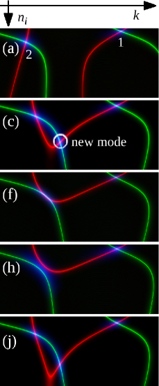
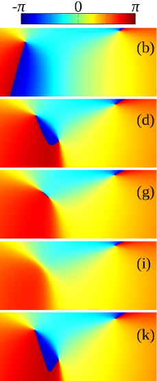
Figure 1: (Color online) Left column: Real (green) and Imaginary (red) zero lines of $M_{22}$ in the $(k,n_{i})$ plane. Right column: Phase $\theta$ of $M_{22}$ in the $(k,n_{i})$ plane. The horizontal axis is real wavenumber $k$ in the range $10.48$ $\mu$m^-1 and $10.64$ $\mu$m^-1. The vertical axis is the imaginary part of refractive index $n_{i}$ in the range -0.0130 and -0.0326. The length $l_{G}$ of the gain region is from top to bottom: (a-b) $14.961$ $\mu$m, (c-d) $14.559$ $\mu$m, (f-g) $14.523$ $\mu$m, (h-i) $14.472$ $\mu$m, (j-k) $14.295$ $\mu$m.

Lasing frequencies and thresholds (gain required to induce lasing) are located by determining which values of $k$ and $n_{i}$, respectively, satisfy $M_{22}=0$. $\operatorname{Re}[M_{22}]=0$ ($\operatorname{Im}[M_{22}]=0$) forms real (imaginary) “zero lines” in the ($k$, $n_{i}$) plane. The crossing of a real and imaginary zero line results in $M_{22}=0$ at that location, thus pinpointing a solution. We visualize these zero lines in Fig. 1 by plotting $-\log_{10}\left|\operatorname{Re}M_{22}\right|$ and $-\log_{10}\left|\operatorname{Im}M_{22}\right|$ together and using image processing techniques to enhance the contrast. We monitor the changes of such zero lines as the gain edge is moved gradually from $l_{G}=L$ (uniform gain) within the wavelength range 500 nm $<\lambda<$ 750 nm. Appearances of new lasing modes with frequencies in between those of the lasing modes with uniform gain are observed. Figure 1 concentrates on a smaller frequency range with Fig. 1(a) showing two of the lasing modes (marked mode 1 and mode 2) resulting from the crossing of zero lines for $l_{G}=14.961$ $\mu$m. Mode 1 at $\lambda_{1}=592.6$ nm has a lower lasing threshold than mode 2 at $\lambda_{2}=598.0$ nm. They are the only two lasing modes found within this frequency range and their frequencies are almost the same as those of the corresponding resonant modes of the passive system. As $l_{G}$ is decreased, the lasing modes do not shift much in frequency. However, when $l_{G}=14.559$ $\mu$m, the zero lines are joined as shown in Fig. 1(c). A new lasing mode, encircled in white, appears in between modes 1 and 2. The spatial intensity distribution of the new lasing mode differs from those of modes 1 and 2. As $l_{G}$ decreases further, the zero lines forming mode 2 and the new mode pull apart. This causes the solutions to approach each other in the ($k$, $n_{i}$) plane, seen in Fig. 1(f), until becoming identical. The zero lines then separate resulting in the disappearance of mode 2 and the new mode as evidenced by Fig. 1(h). The lines cross again for $l_{G}=14.295$ $\mu$m and the solutions reappear and move away from each other in the ($k$, $n_{i}$) plane in Fig. 1(j).

Verification of lasing mode solutions is provided by the phase of $M_{22}$, calculated as $\theta=\operatorname{atan2}(\operatorname{Im}[M_{22}],\operatorname{Re}[M_{22}])$. Locations of vanishing $M_{22}$ give rise to phase singularities. The phase change around a closed path surrounding a singularity is referred to as topological charge Halperin (1981); Zhang et al. (2007). Two phase singularities are seen in Fig. 1(b) at the same locations as the zero line crossings in Fig. 1(a). This verifies the authenticity of the lasing mode solutions. The phase singularity at the location of the new mode in the ($k$, $n_{i}$) plane [Fig. 1(d)] confirms that it is a genuine lasing mode in the presence of linear gain. The phase singularity associated with the new mode is of opposite charge to the existing ones. As $l_{G}$ is reduced, two oppositely charged phase singularities move closer [Fig. 1(g)] and eventually annihilate each other at $l_{G}=14.295$ $\mu$m [Fig. 1(i)]. As already mentioned, this process reverses itself and the two lasing modes reappear in Fig. 1(k).

For a more thorough study of the new lasing modes and confirmation of their existence in the presence of gain saturation, we switch to a more realistic gain model including nonlinearity. The Bloch equations for the density of states of two-level atoms Ziolkowski et al. (1995) are solved together with the Maxwell’s equations with the finite-difference time-domain method tafl05 . The phenomenological decay times due to the excited state’s lifetime $T_{1}$ and decoherence $T_{2}$ are included. The gain spectral width is given by $\Delta\omega_{a}=1/T_{1}+2/T_{2}$ Siegman (1986). We also include incoherent pumping of atoms. The rate of atoms being pumped from the ground state to the excited state is proportional to the ground state population, and the proportional coefficient $P_{r}$ is called the pumping rate. The resulting Maxwell-Bloch (MB) equations are solved numerically with the spatial grid step $\Delta x=1.0$ nm and the temporal step $\Delta t=3.3\times 10^{-18}$ s. The atomic density $N_{atom}/V=1.8\times 10^{13}$ cm^-3. Nonuniform gain is simulated by having the two-level atoms only in the region $0\leq x\leq l_{G}$.

By setting the atomic transition wavelength $\lambda_{a}$ to coincide with the wavelength of mode 1, 2 or the new mode and using a narrow gain spectrum, we are able to investigate the three lasing modes separately. $\Delta\omega_{a}$ is chosen to be less than the mode spacing to ensure single mode lasing (at smaller pumping rates). At $l_{G}=14.295$ $\mu$m, the wavelength difference between mode 2 and the new mode, which is smaller than that between mode 1 and the new mode, is $\lambda_{2}-\lambda_{nm}=1.4$ nm. We set $T_{1}=1.0\times 10^{-12}$ s and $T_{2}=0.73\times 10^{-12}$ s so that the gain spectral width in terms of wavelength is $\Delta\lambda_{a}=0.71$ nm. Initially all atoms are in their ground state and the system is excited by a Gaussian-sinusoidal pulse with center wavelength $\lambda_{0}=\lambda_{a}$ and spectral width $\Delta\lambda_{0}=\Delta\lambda_{a}$. When the pumping rate $P_{r}$ is above a threshold value, the electromagnetic fields build up inside the system until a steady state is reached.

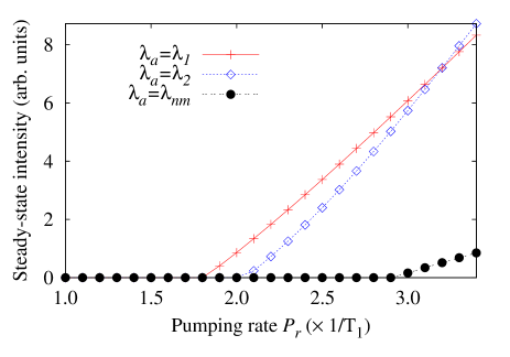
Figure 2: (Color online) Steady-state output intensity vs. pumping rate $P_{r}$ from Maxwell-Bloch simulations with different gain spectra. The wavelength of the atomic transition $\lambda_{a}$ is equal to $\lambda_{1}$ (red crosses), $\lambda_{2}$ (blue open diamonds), and $\lambda_{nm}$ (black circles).

Figure 2 shows the steady-state output intensity with $\lambda_{a}=\lambda_{1}$, $\lambda_{2}$, or $\lambda_{nm}$ as $P_{r}$ is varied. $P_{r}=1/T_{1}$ corresponds to the transparency point, namely, the excited state population of atoms is equal to that of the ground state. The lasing threshold pumping rate for mode 1 is reached first at $P_{r}=1.9/T_{1}$, then mode 2 at $P_{r}=2.1/T_{1}$ and the new mode at $P_{r}=3.0/T_{1}$. These thresholds agree qualitatively with the values of the TM calculation.

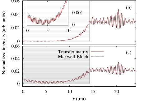
Figure 3: (Color online) (a) Emission spectra taken from two Maxwell-Bloch simulations with $\lambda_{a}$ equal to $\lambda_{nm}$ (solid line) and $\lambda_{2}$ (dashed line). In both cases, $\Delta\lambda_{a}=0.71$ nm, $l_{G}=14.295$ $\mu$m. $P_{r}=3.0/T_{1}$ for the solid curve and $2.1/T_{1}$ for the dashed curve. The emission intensity reaches a steady state by a simulation time of $t=300\times 10^{-12}$ s. The spectra are taken from $1400\times 10^{-12}$ s to $1700\times 10^{-12}$ s. The MB intensity distribution $|\phi_{MB}(x)|^{2}$ (black dashed line) is compared to the TM intensity distribution $|\phi_{TM}(x)|^{2}$ (red solid line) for the new lasing mode (b) and mode 2 (c). The inset in (b) is an expansion of the curves for 0 $\mu$m $<x<10$ $\mu$m.

When $\lambda_{a}=\lambda_{nm}$, the first lasing mode is the new mode, instead of mode 1 or 2. Figure 3(a) shows the output emission spectrum just above the lasing threshold at $P_{r}=3.0/T_{1}$. It consists of a single lasing mode with the wavelength equal to that of the new mode calculated with the TM method. The spatial intensity distribution obtained from the Maxwell-Bloch (MB) calculation is compared to that from the TM calculation in Fig. 3(b). The MB distribution $|\phi_{MB}(x)|^{2}$ is found by integrating the intensity over one optical period. It is then normalized to the TM distribution $|\phi_{TM}(x)|^{2}$ as $\int_{0}^{L}|\phi_{MB}(x)|^{2}dx=\int_{0}^{L}|\phi_{TM}(x)|^{2}dx$. The two intensity distributions are almost identical. The average percent difference between them is 7.77%. This result indicates the nonlinear effect due to gain saturation is small when the pumping rate is just above the lasing threshold. When the peak of the gain spectrum is shifted from $\lambda_{nm}$ to $\lambda_{1}$ or $\lambda_{2}$, the first lasing mode is switched to mode 1 or 2. Figure 3(c) plots the spatial intensity distribution of mode 2 obtained by the MB calculation with $\lambda_{a}=\lambda_{2}$ and $P_{r}=2.1/T_{1}$ as well as that obtained by the TM calculation. The two distributions are almost the same and they are different from the distribution with uniform gain. Comparing Fig. 3(b) to (c), we see the spatial intensity distribution of the new lasing mode differs significantly from that of mode 2 within the gain region. Outside the gain region the two distributions are not much different because their wavelengths are very close.

When optical gain is located on the left side of the structure, we observe that the intensity distributions of new lasing modes are heavily concentrated on the right side of the gain region. This makes the emission intensity through the right boundary of the random system much larger than that through the left boundary. We calculate the the ratio of right to left output flux $S\equiv|\phi(x=L)|^{2}/|\phi(x=0)|^{2}$. For the new lasing mode in Fig. 3(b) $S_{nm}=40$, indicating the laser output is mostly to the right. As a comparison, $S_{1}=1.1$ for mode 1 and $S_{2}=3.3$ for mode 2. Thus, the new lasing mode has much more directional output than modes 1 and 2.

Because of the excellent agreement found between the MB and TM calculations, we conclude that new lasing modes do appear in random lasers with spatially nonuniform distributions of optical gain. Typically, as in the case studied here, they are sensitive to the spatial gain distribution and disappear if the distribution is altered slightly. These new lasing modes offer more control of random laser performance as their properties such as frequency and output directionality can be quite different from those of existing lasing modes. Moreover, the properties of new lasing modes can be easily altered by varying the spatial profile of the pump beam, without modifying the random structures.

The authors thank Christian Vanneste, Patrick Sebbah, Li Ge, A. Douglas Stone, Jan Wiersig, and Dimitry Savin for stimulating discussions, and acknowledge support from the Yale Faculty of Arts and Sciences HPC facility and staff. This work was supported partly by the National Science Foundation under Grant Nos. DMR-0814025 and DMR-0808937.

References

- Siegman (1986) A. E. Siegman, Lasers (University Science Books, Mill Valley, 1986).
- Horowicz et al. (1992) R. J. Horowicz, H. Heitmann, Y. Kadota, and Y. Yamamoto, Appl. Phys. Lett. 61, 393 (1992).
- Gmachl et al. (1998) C. Gmachl, F. Capasso, E. E. Narimanov, J. U. Nöckel, A. D. Stone, J. Faist, D. L. Sivco, and A. Y. Cho, Science 280, 1556 (1998).
- Fukushima et al. (2002) T. Fukushima, T. Harayama, P. Davis, P. O. Vaccaro, T. Nishimura, and T. Aida, Opt. Lett. 27, 1430 (2002).
- Chern et al. (2003) G. D. Chern, H. E. Türeci, A. D. Stone, R. K. Chang, M. Kneissl, and N. M. Johnson, Appl. Phys. Lett. 83, 1710 (2003).
- Hentschel and Kwon (2009) M. Hentschel and T. Y. Kwon, Opt. Lett. 34, 163 (2009).
- Wu et al. (2004) X. H. Wu, A. Yamilov, H. Noh, H. Cao, E. W. Seelig, and R. P. H. Chang, J. Opt. Soc. Am. B 21, 159 (2004).
- Vanneste and Sebbah (2005) C. Vanneste and P. Sebbah, Phys. Rev. E 71, 026612 (2005).
- Gottardo et al. (2008) S. Gottardo, R. Sapienza, P. D. García, A. Blanco, D. S. Wiersma, and C. López, Nat. Photonics 2, 429 (2008).
- García et al. (2009a) P. D. García, M. Ibisate, R. Sapienza, D. S. Wiersma, and C. López, Phys. Rev. A 80, 013833 (2009a).
- García et al. (2009b) P. D. García, R. Sapienza, and C. López, Adv. Mater. 21, 1 (2009b).
- Ripoll et al. (2004) J. Ripoll, C. M. Soukoulis, and E. N. Economou, J. Opt. Soc. Am. B 21, 141 (2004).
- Savels et al. (2007) T. Savels, A. P. Mosk, and A. Lagendijk, Phys. Rev. Lett. 98, 103601 (2007).
- Wiersma and Cavalieri (2001) D. S. Wiersma and S. Cavalieri, Nature 414, 708 (2001).
- Lee and Lawandy (2002) K. Lee and N. M. Lawandy, Opt. Commun. 203, 169 (2002).
- Gottardo et al. (2004) S. Gottardo, S. Cavalieri, O. Yaroshchuk, and D. S. Wiersma, Phys. Rev. Lett. 93, 263901 (2004).
- Fujiwara et al. (2009) H. Fujiwara, Y. Hamabata, and K. Sasaki, Opt. Express 17, 3970 (2009).
- Sebbah and Vanneste (2002) P. Sebbah and C. Vanneste, Phys. Rev. B 66, 144202 (2002).
- Türeci et al. (2008) H. E. Türeci, L. Ge, S. Rotter, and A. D. Stone, Science 320, 643 (2008).
- Yamilov et al. (2005) A. Yamilov, X. Wu, H. Cao, and A. L. Burin, Opt. Lett. 30, 2430 (2005).
- Polson and Vardeny (2005) R. C. Polson and Z. V. Vardeny, Phys. Rev. B 71, 045205 (2005).
- Wu et al. (2006) X. Wu, A. Yamilov, A. A. Chabanov, A. A. Asatryan, L. C. Botten, and H. Cao, Phys. Rev. A 74, 053812 (2006).
- Wu et al. (2007) X. Wu, J. Andreasen, H. Cao, and A. Yamilov, J. Opt. Soc. Am. B 24, A26 (2007).
- Deych (2005) L. Deych, Phys. Rev. Lett. 95, 043902 (2005).
- Zhang et al. (2007) S. Zhang, B. Hu, Y. Lockerman, P. Sebbah, and A. Z. Genack, J. Opt. Soc. Am. A 24, A33 (2007).
- Halperin (1981) B. I. Halperin, in Physics of Defects, edited by R. Balian, M. Kleman, and J. P. Poirier (North-Holland, Amsterdam, 1981).
- Ziolkowski et al. (1995) R. W. Ziolkowski, J. M. Arnold, and D. M. Gogny, Phys. Rev. A 52, 3082 (1995).
- (28) A. Taflove and S. Hagness, Computational Electrodynamics (Artech House, Boston, 2005), 3rd ed.