A computational study of the configurational and vibrational contributions to the thermodynamics of substitutional alloys: the $\bf Ni_{3}Al$ case

Abstract

We have developed a methodology to study the thermodynamics of order-disorder transformations in n-component substitutional alloys that combines nonequilibrium methods, which can efficiently compute free energies, with Monte Carlo simulations, in which configurational and vibrational degrees of freedom are simultaneously considered on an equal footing basis. Furthermore, by appropriately constraining the system, we were able to compute the contributions to the vibrational entropy due to bond proportion, atomic size mismatch, and bulk volume effects. We have applied this methodology to calculate configurational and vibrational contributions to the entropy of the $\rm Ni_{3}Al$ alloy as functions of temperature. We found that the bond proportion effect reduces the vibrational entropy at the order-disorder transition, while the size mismatch and the bond proportion effects combined do not change the vibrational entropy at the transition. We also found that the volume increase at the order-disorder transition causes a vibrational entropy increase of $0.08\;\rm{k_{B}/atom}$, which is significant when compared to the configurational entropy increase of $0.27\;\rm{k_{B}/atom}$. Our calculations indicate that the inclusion of vibrations reduces in about 30$\%$ the order-disorder transition temperature determined solely considering the configurational degrees of freedom.

I INTRODUCTION

One of the goals of materials science in the field of alloys is to predict and understand the relative stability of phases characterized by different chemical disorder. The disorder in an alloy can be considered as having a configurational contribution (configurational degrees of freedom), which is the disorder associated to the way the atoms are distributed in the parent lattice; and a vibrational contribution (vibrational degrees of freedom), which is the disorder associated to the phase space region around a static lattice configuration. For a very long time, most theoretical phase diagram calculations were done considering only the configurational degrees of freedom Bragg and Williams (1934); Ducastelle (1991). In the 1990’s, however, several experiments measuring thermodynamical properties of alloys in disordered metastable states,Anthony et al. (1993, 1994); Fultz et al. (1995a); Nagel et al. (1995); Fultz et al. (1995b); Mukherjee et al. (1996); Nagel et al. (1997) demonstrated the existence of a strong interplay between vibrational and configurational degrees of freedom. It became clear that neglecting vibrational contributions to the thermodynamical properties of alloys could lead to inaccuracies, such as differences up to $30\%$ between order-disorder (OD) transition temperatures calculated with and without vibrational degrees of freedom. van de Walle and Ceder (2002) Theoretical studies of these alloys in a metastable disordered phase were performed assuming the alloys to be either completely ordered or totally disordered.Ackland (1994); Althoff et al. (1997); Ravelo et al. (1998); Althoff et al. (1998); van de Walle et al. (1998) The cluster variation method Kikuchi (1951) and its extensions Sanchez et al. (1984) have been used to calculate the configurational contribution in partially disordered systems in equilibrium. Different approaches have been used to incorporate the vibrational degrees of freedom when cluster expansions are used, such as molecular dynamics, Cleri et al. (1993) the coarse graining method, van de Walle and Ceder (2002) and the structure-inversion approach. Connolly and Williams (1983); de Fontaine (1994) In the last two methods, the vibration contribution is taken into account through the harmonic approximation and anharmonicities are included via the quasiharmonic approximation. These two cluster expansion methods allow a first-principles description of the system, however, even calculations within the harmonic approximation are still very demanding for today’s computer capabilities, and approximate approaches are still very useful.Liu et al. (2007) These recent calculationsLiu et al. (2007) have shown that anharmonic effects play an important role in the vibrational contribution to the thermodynamics of alloys. About 10 years ago, a methodology that became known as MCX was proposed to treat simultaneously configurational and vibrational degrees of freedom by means of Monte Carlo simulations, which allow both atomic interchanges and atomic displacements Purton et al. (1998); Barrera et al. (2000); Allan et al. (2001).

In this work, we present a methodology to investigate phase equilibria of alloys that takes into account naturally and simultaneously all configurational and vibrational contributions, including all anharmonicities, through a combination of the MCX approach and efficient tools to determine free energies, namely, the adiabatic switching (AS) Watanabe and Reinhardt (1990) and the reversible scaling (RS)de Koning et al. (1999) methods. An interesting feature of our methodology is that it allows to study the contributions from different vibrational mechanisms to the total vibrational entropy. In real experiments, it is impossible to isolate the many factors that contribute to the vibrational entropy such as the bond proportion, the atomic size mismatch, and the bulk volume mechanisms. On the other hand, it can be done in computer simulations, particularly through the Monte Carlo technique, which makes possible to isolate the constraints associated with each mechanism. For example, the configurational contribution to the entropy can be calculated by allowing only the atomic interchanging dynamics. The effect of the bonds between different atomic species can be simulated by constraining the atoms to vibrate around their ideal crystalline structure positions and allowing the interchanging dynamics. The effect of the atomic size mismatch and the bond proportion mechanisms combined can be simulated by letting the atoms vibrate around their relaxed equilibrium positions at fixed volume and allowing the configurational dynamics. Finally, the volume mechanism can be simulated by allowing the volume of the supercell to vary by imposing constant pressure on the system, in addition to the positional and configurational dynamics. In summary, our methodology allows also to assess the contribution of a given vibrational mechanism by setting the appropriate constraint in the dynamics and then calculating the vibrational entropy difference between the relaxed and unrelaxed system. We have applied this methodology to quantify the vibrational entropy difference at the thermodynamical OD transition of the $\rm Ni_{3}Al$ binary alloy.

We chose the technologically important Liu and Stiegler (1984a, b) $\rm Ni_{3}Al$ as the alloy model for our study mainly because it is supposed to have the largest vibrational entropy difference upon disorder.Anthony et al. (1993); Fultz et al. (1995b); Ackland (1994); Althoff et al. (1997); Ravelo et al. (1998); Althoff et al. (1998); van de Walle and Ceder (2002) The vibrational entropy difference due to disorder at the thermodynamical OD transition should be large enough to be unambiguously detected, since it is, in general, a fraction of the corresponding configurational entropy difference, which is itself relatively small. We also chose $\rm Ni_{3}Al$ because it is particularly suitable to assess the magnitude of the size mismatch effect, since the difference between the atomic volumes of Al and Ni is quite large Morgan et al. (2000) $(V_{Al}-V_{Ni})/(V_{Al}+V_{Ni})/2=0.41$. In the case of $\rm Ni_{3}Al$, most of the research in the field, both experimentalAnthony et al. (1993); Fultz et al. (1995b) and theoretical, either using the embedded atom method Althoff et al. (1997); Ravelo et al. (1998); Althoff et al. (1998) or tight-binding Ackland (1994); Meirelles et al. (2007) potentials, has found a significant vibrational entropy difference between the totally disordered (metastable) and the ordered phases. However, the subject is not free of controversy, van de Walle et al. van de Walle et al. (1998); AnM , using ab initio calculations, found that the totally disordered and the ordered phases have essentially the same vibrational entropy. Our results indicate an increase of $0.08\;\rm{k_{B}/atom}$ in the vibrational entropy at the thermodynamical OD transition, which is significant when compared to the corresponding configurational entropy increase of $0.27\;\rm{k_{B}/atom}$. We have also found that the bond proportion mechanism diminishes the vibrational entropy at the thermodynamical OD transition, whereas the size mismatch mechanism does not change it. These results are consistent with the local entropy calculations of Morgan et al.Morgan et al. (1998, 2000). Regarding the importance of the volume mechanism, theoretical studies Althoff et al. (1997); Ravelo et al. (1998); Althoff et al. (1998); Ackland (1994); Meirelles et al. (2007) have found that the volume mechanism is the main responsible for the increase of the vibrational entropy difference between the totally disordered and the ordered phase. This is supported by experimental work,Gialanella et al. (1992); Cardellini et al. (1993); Zhou et al. (1995) in which it has been found an increase of the volume as the system becomes totally disordered. We have found that the volume increases 1.2$\%$ at the OD thermodynamical transition. In addition, our calculations indicate that the volume mechanism is the responsible for the increase in the vibrational entropy difference at the OD transition.

The paper is organized as follows. In section II we present the general methodology. Section III describes the details of the interatomic potential we have chosen to describe the $\rm Ni_{3}Al$ alloy. In section IV, the methodology is applied to evaluate the configurational and vibrational entropy as function of the temperature and the contribution of each vibrational mechanism at the OD transition. In section V we summarize the results.

II METHODOLOGY

II.1 Dynamics and vibrational mechanisms

In real systems, the process of chemical disordering takes place mainly through the migration of vacancies. Oramus et al. (2001); Kessler et al. (2003) The problem of realistically simulating the disordering process through this mechanism is that the average vacancy concentration is very low (less than $10^{-5}$), de Koning et al. (2002) implying the requirement of very large system sizes. For this reason, we chose the atomic exchange dynamics to simulate the chemical disorder. This dynamics can be implemented through the Monte Carlo method. In this approach, the configurational degrees of freedom are explored by selecting at random two atoms belonging to different chemical species, their positions in the lattice are then interchanged, the energy change upon the atomic exchange is calculated, the Boltzmann factor associated to this change in energy is computed, and the move is accepted or rejected according to the Metropolis algorithm. Newman and Barkema (1999) In order for the algorithm to be efficient, one should keep two lists of atoms of each atomic species and choose randomly one atom of each list to form the pair of atoms to be interchanged. This can be easily done, since the number of atoms of chemical species is kept constant. This dynamics is more efficient than the Kawasaki dynamics and satisfies detailed balance. We will call this dynamics as the configurational case. We consider a Monte Carlo step (MCS) in the configurational case as $N$ attempts to exchange the atomic positions of two atoms of different species chosen at random, where $N$ is the number of atoms.

In order to investigate the various contributions to the vibrational entropy we considered different dynamics related to the various mechanisms we have mentioned earlier. To estimate the effect of the bond proportion mechanism in the vibrational entropy we define the following dynamics: besides the atomic interchange dynamics, we constrain the atoms to vibrate around their ideal crystalline structure positions. We call this dynamics as the unrelaxed case. The vibrational dynamics for the unrelaxed case is accomplished by choosing one atom at random and calculating a new state by

$$x_{i}^{new}=x_{i}^{id}+\Delta_{max}(2\xi_{i}-1),\qquad i=1..3,$$ (1)

where $x_{i}^{id}$ is the coordinate associated to the corresponding ideal crystalline structure position, $\xi_{i}$ is a random number between zero and one, and $\Delta_{max}$ is the maximum displacement allowed, which is adjusted automatically in such a way that $50\%$ of the trials are accepted. Allen and Tildesley (1989) In this case, a MCS was considered as $N$ attempts of atomic displacements followed by $N^{\prime}$ attempts to exchange atoms. We chose $N^{\prime}=N/10$, in the particular case of $\rm Ni_{3}Al$, because it is the minimum number of attempts of atomic exchange needed for the potential energy and the order parameter to relax to average values. The bond proportion mechanism is claimed Morgan et al. (2000, 1998); van de Walle and Ceder (2002) to be relevant for changes in the vibrational entropy due to chemical disorder, since the proportion of bonds between distinct and similar atoms changes with the disorder. This effect could in principle be addressed, from the theoretical point of view, through calculations based on a spring model,Morgan et al. (2000, 1998); van de Walle and Ceder (2002) which presumably assigns a softer and a stiffer character to the bonds between like and unlike atoms, respectively.Ni (3)

We now set a different type of dynamics by letting the atoms relax around their thermal equilibrium position as

$$x_{i}^{new}=x_{i}^{old}+\Delta_{max}(2\xi_{i}-1),\qquad i=1..3.$$ (2)

This kind of dynamics allows the atoms to vibrate around their thermal equilibrium positions, taking into account naturally their accommodation due to their different atomic sizes. This is another mechanism that is claimed to influence the vibrational entropy and is called the size mismatch mechanism. It can be understood by the following picture:van de Walle and Ceder (2002) when two large atoms are constrained in a small space they can experience a compressive stress, increasing the stiffness of the bond, and reducing the allowed region to vibrate; on the other hand, when two small atoms are constrained in the same space they can experience a tensile stress, increasing the softness of the bond, and increasing the allowed region to vibrate. The interplay between the compressive and tensile stresses will dictate the final vibrational effect. We call this relaxation of the configurational and positional constraints as the partially relaxed case. With this dynamics we simulate the combined effect of bond proportion and size mismatch in the vibrational entropy. In this case also, a MCS was considered to be the same as in the unrelaxed case.

Finally, we simulate the contribution from the volume mechanism by allowing the volume change in a constant pressure simulation. This effect is explained van de Walle and Ceder (2002) by the following reasoning: as the average interatomic distances increase, the bonds become softer and the atoms have more space to visit, that causes an increase in the vibrational entropy. We call this relaxation of the configurational, positional, and volumetric constraints as the fully relaxed case. Through this dynamics we simulate the combined effect of the bond proportion, size mismatch, and volume mechanisms in the vibrational entropy. The volumetric dynamics is accomplished by rescaling the atomic positions according to the volume change calculated as

$$L^{new}=L^{old}+\Delta_{max}^{L}(2\xi-1),$$ (3)

where $L$ is the length of the simulation box, and $\Delta_{max}^{L}$ is the maximum allowed change in that length, which is adjusted similarly to the unrelaxed and partially relaxed cases at typically 10 MCS. In the fully relaxed case, a MCS was defined as $N$ positional trials followed by $N^{\prime}=N/10$ exchanging trials, and one volumetric trial.Allen and Tildesley (1989)

II.2 Free energy calculations

The thermodynamical quantity that underlies all this work is the free energy, which is calculated through the AS Watanabe and Reinhardt (1990) and RS de Koning et al. (1999) methods. The AS method allows one to calculate the free energy by computing the work done by adiabatically switching the Hamiltonian of the system of interest to the Hamiltonian of a reference system (or vice-versa) at a single given temperature. On the other hand, the RS method allows one to evaluate the free energy in a range of temperatures provided that it is known at a single given temperature. These methods are very efficient since they evaluate the free energy from only one simulation run, whose length is determined by the required accuracy. In contrast with other methods, such as the harmonic,Maradudin et al. (1971) or the quasi-harmonic Althoff et al. (1997, 1998); van de Walle et al. (1998) approximations, the AS and RS, take into account naturally all anharmonic effects, which are crucial for the calculation of vibrational entropy differences.

The AS method is based on the well known thermodynamic integration method (TI).Frenkel and Smit (2001) In the TI method, the absolute free energy of a system of interest can be estimated by computing the work done to transform the Hamiltonian of a reference system, of which one knows the free energy, into that of the system of interest. This can be achieved by considering the artificial Hamiltonian, $H(\lambda)=\lambda H_{sys}+(1-\lambda)H_{ref}$, where $H_{sys}$ is the Hamiltonian of the system of interest, $H_{ref}$ is the Hamiltonian of the reference system, and $\lambda$ is a dimensionless coupling parameter. By varying $\lambda$ from 0 to 1, one can transform one Hamiltonian into the other one. The work performed to switch between the two systems is given by the integral

$$F-F_{ref}=\int_{0}^{1}d\lambda\left\langle\frac{\partial H}{\partial\lambda}\right\rangle_{\lambda}.$$ (4)

If now $\lambda$ is considered to be a function of time, and its value continuously varied from 0 to 1 during the time of simulation $t_{s}$, the free energy difference between the two systems is given by

$$F-F_{ref}=\int_{0}^{t_{s}}dt\frac{d\lambda}{dt}(U_{sys}-U_{ref})=W_{irr}=W_{rev}+E_{diss},$$ (5)

where $U_{sys}$ is the potential energy of the system of interest, $U_{ref}$ is the potential energy of the reference system, $W_{irr}$ and $W_{rev}$ are the irreversible and reversible work, respectively, and $E_{diss}$ is the energy dissipation. Time in Eq.(5) can be regarded as the actual time, as in a molecular dynamics simulation, or the fictitious time created by the successive steps in a Monte Carlo simulation. The potential energy difference between the reference system and the system of interest appears in Eq.(5), instead of the Hamiltonian difference, because we consider the kinetic degrees of freedom to be in equilibrium, and, therefore, the kinetic energy terms cancel each other. The energy dissipation is one source of error, characteristic of nonequilibrium dynamic processes, and can be estimated de Koning et al. (2000) by performing the direct and inverse transformations between the two systems:

$$E_{diss}=\frac{W_{irr}^{ref\rightarrow sys}+W_{irr}^{sys\rightarrow ref}}{2}.$$ (6)

In all AS and RS calculations we adopted this criterion to quantify the free energy error, which can be reduced by increasing the simulation time. Another source of error de Koning et al. (2000) are the statistical fluctuations of the quantities in the integrand of Eq.(5), which can be handled by simulating other trajectories and averaging the results.

There are subtleties in the AS method we must be aware of in order to obtain the correct free energy. The external conditions, like temperature, and the parameters of the reference system must be set in a way that the coupled system, described by $H(\lambda)$, does not undergo a phase transition along the transformation path. (We took particular care about the choice of the reference temperature for the high temperature disordered phases in the unrelaxed, partially relaxed, and fully relaxed cases to avoid mechanical melting.)

Now let us discuss briefly the RS method and its application.de Koning et al. (1999) In contrast to the AS, the RS method allows the calculation of the free energy in a range of temperatures. This can be accomplished by realizing that the free energy of the scaled system at a temperature $T_{0}$, whose potential energy is given by $U_{scaled}=\lambda U_{sys}$ (in the case of RS $\lambda$ is not restricted to the interval $[0,1]$), is related to the free energy of our system of interest at a temperature $T=T_{0}/\lambda$.de Koning et al. (1999, 2000) The free energy of the scaled system at a given value of $\lambda$ can be readily determined by computing the work performed to change $\lambda$ from 1 to $\lambda=T_{0}/T$, as it is done in the AS method (provided that the free energy is known for $\lambda=1$). It is shown in Ref. de Koning et al., 1999 that the free energy of a system at temperature $T$ can be estimated from the irreversible work $W_{irr}(t)$ done to bring the system from $T_{0}$ to $T(t)$, as

$$\frac{F(T(t))}{T(t)}=\frac{F(T_{0})}{T_{0}}+\frac{W_{irr}(t)}{T_{0}}-\frac{3}{2}k_{B}N\ln\frac{T(t)}{T_{0}},$$ (7)

where $T(t)=T_{0}/\lambda(t)$, and $F(T_{0})$ is the known free energy reference. The logarithmic term of Eq.(7) corresponds to the contribution of the kinetic degrees of freedom and must be omitted when only the configurational changes are considered. The estimation of the energy dissipation at a given temperature is calculated, as in the AS method, using Eq.(6). In the case where the external pressure is set zero, as in the calculation of the free energies for the fully relaxed case, the Gibbs free energy formula reduces to Eq.(7).

III THE $\rm\bf Ni_{3}Al$ SYSTEM

III.1 The choice of potential

Some well known and often used interatomic potentials for modeling $\rm Ni_{3}Al$ Cleri and Rosato (1993); Papanicolaou et al. (2003) are not suitable to describe the configurational degrees of freedom of this alloy.Michelon and Antonelli (2008) The reason for that is that this potential, in both parameterizations,Cleri and Rosato (1993); Papanicolaou et al. (2003) does not yield the $L1_{2}$ phase as the ground state phase, giving rise to nonphysical thermodynamical phases at low temperatures.Michelon and Antonelli (2008) In order to modeling appropriately the $\rm Ni_{3}Al$ system we looked for a potential which provides not only the correct ground state, but describes, at least qualitatively, the thermodynamics of the OD and vibrational phenomena. We chose the tight-binding Finnis-Sinclair Finnis and Sinclair (1984) potential whose parameterization was obtained by Vitek et al.Vitek et al. (1991) Among the thermal features of this potential we may cite the linear thermal expansion coefficient (at 1050 K) of $21.7\times 10^{-6}\rm{K}^{-1}$, which agrees well with the experimental value of $19\times 10^{-6}\rm{K}^{-1}$; Rao et al. (1989) the equilibrium lattice parameter (at 1000 K) of $a_{0}=3.6096$ Å, which is in good agreement with the experimental value of $a_{0}=3.6120$ Å;Rao et al. (1989) and the calculated mechanical melting temperature $T_{m}^{mech}=1600\pm 25$ K at the Lindemanns’$\delta$ function value of $0.12$. We have determined the thermodynamical melting temperature for this model of $\rm Ni_{3}Al$ to be $T_{m}=1328\pm 6$ K. The thermodynamical melting point of a substance is obtained by determining at which temperature the solid and liquid phases have the same free energy. It is important to point out that the thermodynamical melting temperature we have obtained for the model is 20$\%$ lower than the experimental value $T_{m}^{exp}=1636$ K. Bremer et al. (1988) This discrepancy in the melting transition temperature is not surprising since the potential parameters are fitted from a database which does not include data from the liquid phase. We will return to this point later, after we present the results for the OD transition. However, the important conclusion we should advance at this point is that, despite numerical discrepancies, the results from our simulations for the OD transition temperature and the melting point are qualitatively consistent with experimental findings.

III.2 Order parameters

In the case of $L1_{2}$ alloys, the order parameters can be defined as follows. The long-range order parameter is constructed from the $L1_{2}$ phase by labeling the sublattice associated to the Al (Ni) atom as an $\alpha$ ($\beta$) sublattice. The long-range order is then measured by the formula, first introduced by Bragg and Williams, Bragg and Williams (1934)

$$\eta=\frac{p_{\alpha}-0.25}{1-0.25},$$ (8)

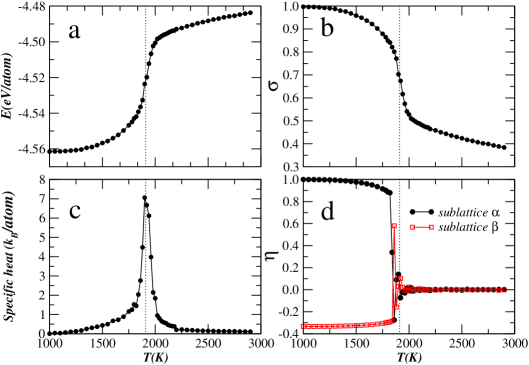
Figure 1: (Color online) Thermal equilibrium quantities for the configurational case. The dotted lines indicate the OD temperature calculated from free energy calculations(Fig.2). The order parameter $\eta$ is shown for two of the four sublattices of the $L1_{2}$ structure, the order parameters not shown exhibit an identical behavior to that of sublattice $\beta$.

where $p_{\alpha}$ means the fraction of Al atoms in the $\alpha$ sublattice. In this way, $\eta=1$ for the ordered $L1_{2}$ phase and $\eta=0$ for the disordered phase. This order parameter is very useful to quantify the long-range order, however one must be careful with its interpretation. First, when one performs computer simulations to explore the configurational degrees of freedom through cooling experiments, at a relative low rate, starting from the disordered phase at high temperatures, the system should always end up in the $L1_{2}$ phase, but the Al atoms not always are found in the arbitrarily defined $\alpha$ sublattice. In other words, one does not know, in advance, which one of the four possible sublattices will be $\alpha$ sublattice. Hence, in this kind of experiment one must measure the long-range order parameter in the four possible sublattices. Second, when the system is in an antiphase boundary (APB)-like configuration Michelon and Antonelli (2008) a large fraction of Al atoms may be in a ordered block at sites of a $\beta$ sublattice, giving low and even negative values for $\eta$. Therefore, $\eta=0$ does not distinguish between a totally disordered and a particular APB configuration. In Fig. 1d, we show the results for the long-range order parameter for the $\alpha$ and $\beta$ sublattices.

Concerning the short-range correlations we measure the short-range order parameter, first introduced by Bethe and Wills,Bethe and Wills (1935) as

$$\sigma=\frac{p_{Al-Ni}-9}{12-9},$$ (9)

where $p_{Al-Ni}$ means the average number of unlike bonds between an Al atom and its first-neighbors. Note that $\sigma=0$ implies $\eta=0$, however, $\eta=0$ can correspond to $\sigma=1$ as in a particular APB configuration.

III.3 Implementation details

We have performed tests of our computational code by calculating the melting temperature of the Ni system using the Cleri and Rosato potential, Cleri and Rosato (1993) which agrees exactly with the value reported in Ref. Bedoya-Mart nez et al., 2006. Furthermore we compared our Finnis-Sinclair calculations of antiphase-boundary and stacking fault energies with Vitek et al. Vitek et al. (1991) results, and verified an exact agreement.

The reference system chosen for the calculation of free energy references in the solid phases was the Einstein crystal.de Koning and Antonelli (1996, 1997); Frenkel and Smit (2001) The chosen values for the vibration angular frequencies are $w_{Al}=75.4$ rad THz, and $w_{Ni}=31.4$ rad THz, for the Al atom and for the Ni atom respectively. These are the frequencies of the main vibrational modes of the elements, estimated from the experimental phonon density of states from Ref. Stassis et al., 1981, which are expected to be optimal to mimic the vibration of the atoms in the alloy. The reference system chosen for the calculation of the free energy reference of the liquid phase (used to estimate the melting temperature) was the $r^{-12}$ repulsive fluid.Hoover et al. (1971); Young and Rogers (1984) The repulsive fluid parameters are chosen in such a way that the position and height of the first peak of the radial distribution function of the $r^{-12}$ repulsive fluid potential coincide with those of the Finnis-Sinclair potential. This choice of parameters enhances the probability of the reference system to be within the borders of the phase diagram of the system of interest, thus minimizing the risk of encountering a phase transition.Hoover et al. (1971); Kaczmarski et al. (2004); Bedoya-Mart nez et al. (2006)

In the AS and RS calculations we chose time simulations such that the energy dissipation was less than $10^{-4}\;\rm{eV/atom}$, which typically leads to simulation lengths of $2\times 10^{5}$ MCS. The functional form of $\lambda(t)$ was always chosen to be a linear interpolation between the initial and final simulation times, which correspond to the initial and final temperatures. To circumvent surface effects we applied periodic boundary conditions and the minimal image convention. Allen and Tildesley (1989) Since both, the Einstein crystal and the $r^{-12}$ repulsive fluid do not have any cohesion, the simulations involving these systems have to be performed at fixed volume, which is chosen to be the average volume of a NPT equilibrium simulation at the given pressure and temperature of interest. Aside from the systematic errors due to dissipation, statistical errors in free energy calculations were handled by taking averages over typically 10 samples. The error bars in the entropy differences were obtained from the fluctuation of entropy data below and above the transition in the standard way. In most of the results that will be presented in the following section, a simple running average smoothing procedure was used in order to remove the unwanted fluctuations introduced by the numerical derivative calculations. All the calculations were performed using a cubic simulation cell containing 500 atoms. Finally, we tested a larger system size using a 1372-atom simulation cell and found no significant finite-size effects in entropy differences and transition temperatures.

IV RESULTS AND DISCUSSION

IV.1 The configurational case

Let us discuss briefly the equilibrium numerical experiments performed in order to bracket the OD temperature for the configurational case. We set the $L1_{2}$ phase at a fixed volume corresponding to the equilibrium volume obtained at zero pressure and $T_{0}=10^{3}$ K. Then we turned on the exchange dynamics and performed a series of equilibrium simulations on a relatively fine grid over a temperature interval of 2000 K. The measured thermodynamical quantities are shown in Fig. 1. The abrupt changes in the behavior of the potential energy, specific heat, and order parameters indicate the OD transition at $T_{od}^{conf}=1925\pm 30$ K. Note the abrupt change of the long-range order parameter $\eta$, and the nonzero value of $\sigma$ after the transition. In order to estimate the effect of the chosen fixed volume on our results, we performed an analogous series of calculations at the equilibrium volume at 0 K, which is substantially smaller than the one at zero pressure and $T_{0}=10^{3}$ K. We found the OD transition to be only 5% larger than the previous one, and such small difference indicates that the chosen value for the volume is not relevant for our conclusions.

We now discuss the free energy calculations. We consider the free energy reference in this case to be at infinite temperature, because in this limit the configurational entropy per atom of a system with N atoms has an analytical expression corresponding to the ideal solid solution, which is

$$S_{conf}(\infty)={\frac{1}{N}}k_{B}{\rm ln}\frac{N!}{N_{Al}!N_{Ni}!}.$$ (10)

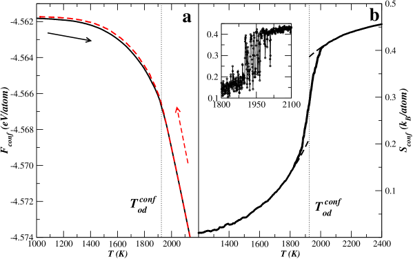
Figure 2: (Color online) Helmholtz free energy and entropy versus temperature for the configurational case. In (a) the solid line and the dashed line correspond to single realizations of the quasi-static heating and cooling processes, respectively. In (b) solid line depicts the entropy obtained from smoothing the $-d\langle F_{conf}\rangle/dT$ data, dashed lines correspond to the coexistence region, and the OD transition temperature $T_{od}^{conf}=1925\pm 30\rm{K}$ is estimated from the center of the coexistence region. The inset shows the entropy of a typical single realization where the coexistence behavior can be observed.

This quantity measures the number of distinct configurations obtained by arranging $N_{Al}$ and $N_{Ni}$ atoms in the lattice. Thus, for a system containing 500 atoms, we have approximately $S_{conf}(\infty)=0.556\;\rm k_{B}/atom$. The advantage of using the RS method in this case results from the fact that the method maps the problem of determining the free energy for an infinite interval of temperature onto a problem of finding the free energy for a finite interval of the scaling parameter $\lambda$. We determine the work done to take the system from $T_{0}=10^{3}$ K ($\lambda=1$) to the virtually infinite temperature ($\lambda=0$). Combining this work and the entropy from Eq.(10), we are able to calculate the free energy at $T_{0}$ using Eq.(7), noting that in the configurational case the logarithmic term should be dropped, since in this case the atoms are not allowed to vibrate. From the free energy reference at $T_{0}$ and by computing the work done to take the system from $\lambda=1$ to any $\lambda<1$, we are able to calculate F as a function of T as shown in Fig. 2.

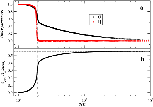
Figure 3: (Color online) Behavior of the order parameters and entropy as functions of temperature in a logarithmic scale for the configurational case. In (a) the long-range order parameter $\eta$ vanishes at the OD transition, in contrast to the short-range order parameter $\sigma$, which vanishes only at very high temperatures. This behavior is reflected in the configurational entropy showed in (b). The dashed line in (b) indicates the value of $S_{conf}(\infty)$.

In order to estimate the energy dissipation we compute the work performed to take the system from $\lambda=0$ (infinite temperature) to $\lambda=1$ ($T_{0}$). As we can see in Fig. 2a the energy dissipation in the direct and reverse processes is less than $10^{-4}\;\rm{eV/atom}$. The configurational entropy, shown in Fig. 2b, is obtained by computing numerically $-d\langle F_{conf}\rangle/dT$, where the brackets denote an average over uncorrelated samples of the configurational free energy. This averaging procedure is done in order to reduce the statistical noise in the numerical derivative (subsequently the remaining noise is further reduced by applying a running average smoothing procedure). The OD transition temperature, which in this case is considered to be at the center of the coexistence region of the two phases, was found to be $T_{od}^{conf}=1925\pm 30$ K, which agrees with the transition temperature determined by analyzing the behavior of thermodynamical quantities in Fig. 1. The configurational entropy difference calculated at the OD transition is $\Delta S^{conf}_{conf}=0.18\pm 0.01\;\rm{k_{B}/atom}$. In Fig. 3a we show the behavior of the order parameters as function of the temperature. We can see that the long-range order parameter goes to zero at the OD transition temperature, whereas the short-range remains finite above the transition, approaching zero only for extremely high temperatures. Due to the persistence of the short-range order, we note that the configurational entropy reaches its maximum only at very high temperatures. The similar behavior of the configurational entropy and short-range order parameter with temperature allows us to establish a direct relationship between these two magnitudes. This relationship will be used in the calculation of free energy references for the other cases we will study. This result may also be especially useful at much higher pressures where the OD temperature is much lower than the melting point.Geng et al. (2005)

IV.2 Unrelaxed, partially relaxed, and fully relaxed cases

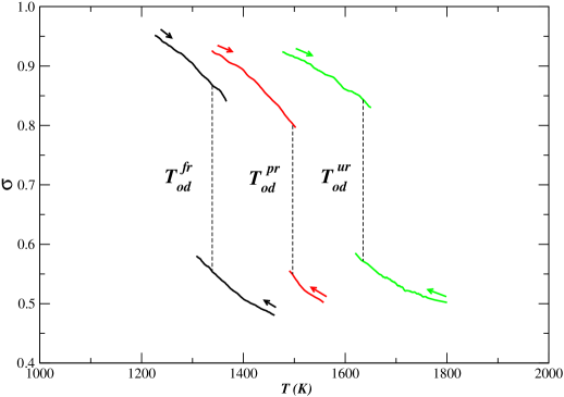
Figure 4: (Color online) Behavior of the short-range order parameter $\sigma$ as a function of temperature in heating and cooling numerical experiments at a rate of 0.02 K/MCS. From left to right, the three pairs of curves are for the fully relaxed, partially relaxed, and unrelaxed cases. The dashed lines indicate the OD transition temperatures, obtained from the crossing of the free energy curves, which are $T_{od}^{fr}=1339\pm 20\;\rm{K}$, $T_{od}^{pr}=1497\pm 40\;\rm{K}$, and $T_{od}^{ur}=1635\pm 60\;\rm{K}$. The curves are the smoothed data from averages over 10 samples.

Now we turn to the other cases, where the constraints on the degrees of freedom are gradually lifted. When vibrations are allowed, the limit of infinite temperature is no longer a suitable reference for the free energy, since the system would not remain a solid. In order to bracket the OD transition temperatures for each case, we performed a series of heating and cooling experiments. In Fig. 4 we plot the short-range order parameter $\sigma$ as a function of the temperature, for the unrelaxed, partially relaxed, and fully relaxed cases. The metastability exhibited in each case allows suitable choices of reference temperatures for the calculation of reference free energies using the AS method. For each case, two reference temperatures are chosen, one below and one above the guessed OD transition temperature provided by the metastability region. These free energy references are subsequently used in the RS method to calculate the free energy curves starting from both reference temperatures. Starting at the lower reference temperature, the RS method generates a free energy curve for increasing temperatures; from the higher reference temperature, on the other hand, the RS method provides a free energy curve for decreasing temperatures. The crossing of these two curves gives the OD transition temperature. These OD transition temperatures are indicated by dotted lines in Fig. 4. The error bars for the transition temperatures were obtained from the free energy reference error bars in the same way as in Ref. de Koning et al., 2001: the RS method is performed again, this time starting from the extremes of the error bar of free energy reference given by the AS method. The temperature error bar is then obtained by the two crossings points that are the farthest from each other among the four curves intersections around the transition. Next, we discuss the details of these calculations and further results.

The total free energy at the reference temperature $T_{ref}$ for the unrelaxed, partially relaxed, and fully relaxed cases is calculated by adding the contributions from the vibrational and configurational degrees of freedom as

$$F(T_{ref})=F_{vib}(T_{ref})-T_{ref}S_{conf}(\sigma(T_{ref})),$$ (11)

where $F_{vib}(T_{ref})$ is the vibrational free energy calculated through the AS method to a reference system which does not take into account the configurational entropy, e.g., the Einstein Crystal, and $S_{conf}$ is the configurational entropy corresponding to the short-range order parameter at $T_{ref}$. The mapping between $S_{conf}$ and $\sigma$ is obtained from their temperature dependence in the configurational case, using the data given in Fig. 3.

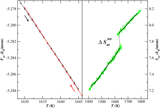
Figure 5: (Color online) Free energy and entropy as functions of temperature for the unrelaxed case. The dashed line indicates the OD temperature of $T_{od}^{ur}=1635\pm 60\;\rm{K}$ obtained from the crossing of the free energy curves. The lines in the entropy plot are obtained from the smoothing of the $-d\langle F_{ur}\rangle/dT$ data.

In order to evaluate the contribution of the bond proportion mechanism to the vibrational entropy, we calculated the free energy of the system in the unrelaxed case. In Fig. 5 we show the free energy and entropy curves below and above the OD transition. The crossing of the two free energy curves determines the OD transition. The entropy is then computed by the numerical derivative of the free energy curves. The OD transition temperature obtained where the two curves cross is $T_{od}^{ur}=1635\pm 60~{}\rm{K}$. Once the transition temperature is obtained, one can go back to the data in Fig. 4 to determine the short-range order parameter for the ordered and disordered phases at the OD transition, and from that the configurational entropy difference at the OD transition. The total entropy difference and the configurational entropy difference at the transition are $\Delta S_{ur}^{tot}=0.20\pm 0.02~{}\rm{k_{B}/atom}$ and $\Delta S_{ur}^{conf}=0.27\pm 0.01\rm{k_{B}/atom}$, respectively. So the entropy difference due to only the vibration

$$\Delta S_{ur}^{vib}=\Delta S_{ur}^{tot}-\Delta S_{ur}^{conf},$$ (12)

is $-0.07\pm 0.02\rm{k_{B}/atom}$. This negative value is consistent with the local entropy calculations of Morgan et al., Morgan et al. (1998, 2000) who concluded that the increase of Al nearest-neighbors decreases the local vibrational entropy of Al or Ni atoms.

The combined effect of size mismatch and the bond proportion mechanisms was studied by simulating the system in the partially relaxed case. The OD temperature obtained by the crossing of the free energy curves is $T_{od}^{pr}=1497\pm 40\;\rm{K}$. The total partially relaxed entropy difference and the configurational entropy difference at the transition are $\Delta S_{pr}^{tot}=0.23\pm 0.02\;\rm{k_{B}/atom}$ and $\Delta S_{pr}^{conf}=0.22\pm 0.01\;\rm{k_{B}/atom}$, respectively. So the entropy difference due to only the relaxation of the atoms at fixed volume is approximately $0.01\pm 0.02\;\rm{k_{B}/atom}$. This result is also consistent with Morgan et al., Morgan et al. (1998, 2000) who observed that the local vibrational entropy “seems very flat, or even slightly increasing” as the number of relaxed Al first-neighbors increases.

Simulations of the system in the fully relaxed case were employed to evaluate the combined effect of the volumetric relaxation of the supercell with the size mismatch and the bond proportion mechanisms. The calculated OD temperature $T_{od}^{fr}=1339\pm 20\;\rm{K}$ essentially coincides, within the error bars, with the melting temperature of $T_{m}=1328\pm 6$ K. This is in agreement with experimental findings.Cahn et al. (1987); Bremer et al. (1988) Although the Finnis-Sinclair potential cannot reproduce quantitatively the values obtained experimentally, it provides results that are consistent with the experimental results.

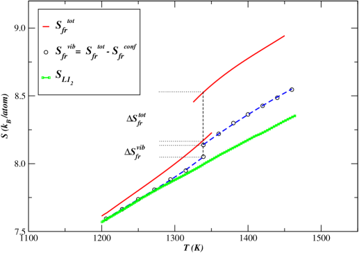
Figure 6: (Color online) Entropy as a function of temperature for the fully relaxed case (solid curve) and perfectly ordered $L1_{2}$ phase (squares). The open circles depict the fully relaxed vibrational entropy, which is the difference between the fully relaxed total entropy and the fully relaxed configurational entropy. The vertical short dashed line indicates the fully relaxed OD temperature. The open circles represent the smoothed data from averages over 10 samples. The solid and long dashed lines are fittings to the smoothed data and the error bars are smaller than the symbols (squares and circles).

In order to show the significance of the configurational disorder on the vibrational properties of the alloy, we depict in Fig.6 the vibrational entropy of the alloy in the fully relaxed case as a function of temperature in comparison with the total entropy of the alloy in the fully relaxed case and in the perfectly ordered $L1_{2}$ phase. In the fully relaxed case the vibrational entropy is obtained by subtracting the configurational entropy from the total entropy. The configurational entropy is, in turn, obtained as a function of temperature from its mapping with the measured short-range parameter. The entropy of the $L1_{2}$ phase is purely vibrational. Therefore, the difference between the fully relaxed vibrational entropy and the $L1_{2}$ vibrational entropy is only due to configurational disorder. We see that, as the temperature increases, the vibrational entropy due to disorder increases steadily and has a finite jump at the OD transition.

The total entropy difference and the configurational entropy difference at the OD transition in the fully relaxed case are $\Delta S_{fr}^{tot}=0.35\pm 0.02~{}\rm{k_{B}/atom}$ and $\Delta S_{fr}^{conf}=0.27\pm 0.01~{}\rm{k_{B}/atom}$, respectively. So the entropy difference excluding the configurational contribution is $\Delta S_{fr}^{vib}~{}=~{}0.08\pm 0.02~{}\rm{k_{B}/atom}$. This result shows that the vibrational entropy difference at the OD temperature is about 23$\%$ of the total entropy difference when the volume is allowed to relax. Furthermore, this vibrational entropy increase is accompanied by a volume increase of 1.2$\%$. This result, together with the essentially zero vibrational entropy difference found in the partially relaxed case, indicates that the volume mechanism is the responsible for the vibrational entropy increase in $\rm Ni_{3}Al$. The increase in volume upon disorder is consistent with all experimental Cardellini et al. (1993); Gialanella et al. (1992); Zhou et al. (1995); ZhZ and theoretical workMeirelles et al. (2007); Ravelo et al. (1998); Althoff et al. (1998); van de Walle et al. (1998); AnM . The result that the vibrational entropy difference increases at the OD transition is consistent with all the experimental Anthony et al. (1993); Fultz et al. (1995b) and most of the theoretical work, Ackland (1994); Meirelles et al. (2007); Althoff et al. (1997); Ravelo et al. (1998); Althoff et al. (1998) which have observed a positive vibrational entropy difference between the totally disordered (metastable) and the totally ordered phases. The OD temperature in the fully relaxed case is approximately 30$\%$ lower than the OD temperature calculated when only the configurational degrees of freedom are considered. Ozoliņš, Wolverton, and Zunger Ozoliņš et al. (1998) proposed a relation between the OD transition temperature calculated considering only the configurational degrees of freedom and the transition temperature determined including also vibrations,

$$T_{od}^{conf+vib}\approx T_{od}^{conf}\left(1+\frac{\Delta S_{fr}^{vib}}{\Delta S_{conf}^{conf}}\right)^{-1}.$$ (13)

Using the results from our calculations as input for Eq. (13), namely, $T_{od}^{conf}=1925~{}\rm K$, $\Delta S_{conf}^{conf}=0.18~{}\rm{k_{B}/atom}$, and $\Delta S_{fr}^{vib}=0.08~{}\rm{k_{B}/atom}$, we find $T_{od}^{conf+vib}=1333~{}\rm K$, i.e., the inclusion of vibrations lowers the OD transition temperature by 31$\%$, with respect to the purely configurational transition temperature, which agrees with the lowering of 30$\%$ we have determined in the fully relaxed case.

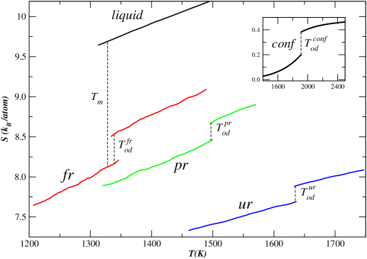
Figure 7: (Color online) Behavior of the total entropy as a function of temperature for the liquid phase and all cases studied. The inset shows the configurational case. The curves are the smoothed data from averages over 10 samples.

Finally, in order to compare the changes in entropy for all cases studied (and also for the liquid phase) we show in Fig. 7 the entropy as a function of the temperature.

V SUMMARY

In this work we employ to the greatest possible advantage the RS and the Monte Carlo techniques, providing a methodology to evaluate both the configurational and vibrational free energies as functions of temperature for n-component substitutional alloys. This methodology is also used to quantify the contributions of the vibrational mechanisms by setting appropriate constraints in the dynamics and calculating the entropy difference between the relaxed and unrelaxed system. By consecutively relaxing the configurational and structural constraints, we are able to quantify the configurational entropy as well as the vibrational entropy due to the bond proportion, size mismatch, and volume mechanisms. We applied this methodology to study the vibrational entropy difference at the thermodynamical OD transition of the $\rm Ni_{3}Al$ alloy obtaining the following results. When the atoms are allowed to both interchange their positions and vibrate around their ideal fcc lattice positions, the vibrational entropy difference is $\Delta S_{ur}^{vib}=-0.07\pm 0.02~{}\rm{k_{B}/atom}$. This indicates that bond proportion mechanism decreases the overall vibration of atoms upon transition. When the atoms can interchange their positions and are allowed to vibrate around their equilibrium positions, the vibrational entropy difference is essentially zero. This indicates that the size mismatch, coupled to the bond proportion mechanism, does not change the vibrational entropy upon transition. When the constraints on atomic interchanging, atomic relaxations, and bulk volume are relaxed, the vibrational entropy difference at the OD transition is $\Delta S_{fr}^{vib}=0.08\pm 0.02\;\rm{k_{B}/atom}$, which is substantial when compared with the configurational entropy difference of $\Delta S_{fr}^{conf}=0.27\pm 0.01\;\rm{k_{B}/atom}$. This indicates that the effect of volume relaxation is the source of the increasing in the overall vibrational entropy upon disorder. Moreover, the volume increase at the OD transition is of 1.2$\%$. A particular relevant result is that the OD transition temperature calculated when all constraints are allowed to relax is approximately 30$\%$ less than that calculated when only the configurational degrees of freedom are considered. This result corroborates the importance of the vibrational degree of freedom in the determination of precise OD phase diagrams. Finally, as this methodology is not restricted to a particular crystal structure and stoichiometry, it can be applied to any n-component substitutional alloy to evaluate the configurational and vibrational entropies as function of the temperature and quantify the importance of the corresponding vibrational mechanisms.

References

- Bragg and Williams (1934) W. L. Bragg and E. J. Williams, Proc. Roy. Soc. A 145, 699 (1934).
- Ducastelle (1991) F. Ducastelle, Order and Phase Stability in Alloys Cohesion and Structure Vol.3 (North-Holland, Amsterdam, 1991).
- Anthony et al. (1993) L. Anthony, J. K. Okamoto, and B. Fultz, Phys. Rev. Lett. 70, 1128 (1993).
- Anthony et al. (1994) L. Anthony, L. J. Nagel, J. K. Okamoto, and B. Fultz, Phys. Rev. Lett. 73, 3034 (1994).
- Fultz et al. (1995a) B. Fultz, L. Anthony, J. L. Robertson, R. M. Nicklow, S. Spooner, and M. Mostoller, Phys. Rev. B 52, 3280 (1995a).
- Nagel et al. (1995) L. J. Nagel, L. Anthony, and B. Fultz, Phil. Mag. Lett. 72, 421 (1995).
- Fultz et al. (1995b) B. Fultz, L. Anthony, L. J. Nagel, R. M. Nicklow, and S. Spooner, Phys. Rev. B 52, 3315 (1995b).
- Mukherjee et al. (1996) G. D. Mukherjee, C. Bansal, and A. Chatterjee, Phys. Rev. Lett. 76, 1876 (1996).
- Nagel et al. (1997) L. J. Nagel, B. Fultz, J. L. Robertson, and S. Spooner, Phys. Rev. B 55, 2903 (1997).
- van de Walle and Ceder (2002) A. van de Walle and G. Ceder, Rev. Mod. Phys. 74, 11 (2002).
- Ackland (1994) G. J. Ackland, in Alloy Modelling and Design, edited by G. Stocks and P. Turchi (The Minerals, Metals, and Materials Society,Warrendale, 1994), p. 149.
- Althoff et al. (1997) J. D. Althoff, D. Morgan, D. de Fontaine, M. Asta, S. M. Foiles, and D. D. Johnson, Phys. Rev. B 56, R5705 (1997).
- Ravelo et al. (1998) R. Ravelo, J. Aguilar, M. Baskes, J. E. Angelo, B. Fultz, and B. L. Holian, Phys. Rev. B 57, 862 (1998).
- Althoff et al. (1998) J. D. Althoff, D. Morgan, D. de Fontaine, M. D. Asta, S. M. Foiles, and D. D.Johnson, Comput. Mater. Science 10, 411 (1998).
- van de Walle et al. (1998) A. van de Walle, G. Ceder, and U. V. Waghmare, Phys. Rev. Lett. 80, 4911 (1998).
- Kikuchi (1951) R. Kikuchi, Phys. Rev. 81, 988 (1951).
- Sanchez et al. (1984) J. M. Sanchez, F. Ducastelle, and D. Gratias, Physica A 128, 334 (1984).
- Cleri et al. (1993) F. Cleri, G. Mazzone, and V. Rosato, Phys. Rev. B 47, 14541 (1993).
- Connolly and Williams (1983) J. W. D. Connolly and A. R. Williams, Phys. Rev. B 27, 5169 (1983).
- de Fontaine (1994) D. de Fontaine, Solid State Phys. 47, 33 (1994).
- Liu et al. (2007) J. Z. Liu, G. Ghosh, A. van de Walle, and M. Asta, Phys. Rev. B 75, 104117 (2007).
- Purton et al. (1998) J. A. Purton, G. D. Barrera, N. L. Allan, and J. D. Blundy, J. Phys. Chem. B 102, 5202 (1998).
- Barrera et al. (2000) G. D. Barrera, R. H. de Tendler, and E. P. Isoardi, Modelling Simul. Mater. Sci. Eng. 8, 389 (2000).
- Allan et al. (2001) N. L. Allan, G. D. Barrera, M. Y. Lavrentiev, I. T. Todorov, and J. A. Purton, J. Mater. Chem. 11, 63 (2001).
- Watanabe and Reinhardt (1990) M. Watanabe and W. P. Reinhardt, Phys. Rev. Lett. 65, 3301 (1990).
- de Koning et al. (1999) M. de Koning, A. Antonelli, and S. Yip, Phys. Rev. Lett. 83, 3973 (1999).
- Liu and Stiegler (1984a) C. T. Liu and J. O. Stiegler, Science 226, 636 (1984a).
- Liu and Stiegler (1984b) C. T. Liu and J. O. Stiegler, Mater. Eng. 100, 29 (1984b).
- Morgan et al. (2000) D. Morgan, A. van de Walle, G. Ceder, J. D. Althoff, and D. de Fontaine, Modelling Simul. Mater. Sci. Eng. 8, 295 (2000).
- Meirelles et al. (2007) B. R. Meirelles, C. R. Miranda, and A. Antonelli, unpublished (2007).
- (31) In the Ref. van de Walle et al., 1998 the authors used a SQS structure to simulate the disorder in an 8-atom supercell. In contrast, the authors in Ref. Meirelles et al., 2007 implemented the disorder directly using a simulated annealing algorithm in a 108-atom supercell and relaxed it using ab initio calculations.
- Morgan et al. (1998) D. Morgan, J. D. Althoff, and D. de Fontaine, J. Phase Equilibria 19, 559 (1998).
- Gialanella et al. (1992) S. Gialanella, S. B. Newcomb, and R. W. Cahn, in Ordering and Disordering in Alloys, edited by A. Yavari (Proc. European Workshop on Ordering and Disordering, Elsevier Applied Science, London, 1992), p. 67.
- Cardellini et al. (1993) F. Cardellini, F. Cleri, G. Mazzone, A. Montone, and V. Rosato, J. Mater. Res. 8, 2504 (1993).
- Zhou et al. (1995) G. F. Zhou, M. J. Zwanenburg, and H. Bakker, J. Appl. Phys. 78, 3438 (1995).
- Oramus et al. (2001) P. Oramus, R. Kozubski, V. Pierron-Bohnes, M. C. Cadeville, and W. Pfeiler, Phys. Rev. B 63, 174109 (2001).
- Kessler et al. (2003) M. Kessler, W. Dieterich, and A. Majhofer, Phys. Rev. B 67, 134201 (2003).
- de Koning et al. (2002) M. de Koning, C. R. Miranda, and A. Antonelli, Phys. Rev. B 66, 104110 (2002).
- Newman and Barkema (1999) M. Newman and G. Barkema, Monte Carlo Methods in Statistical Physics (Clarendon Press, Oxford, 1999).
- Allen and Tildesley (1989) M. P. Allen and D. J. Tildesley, Computer Simulation of Liquids (Oxford University Press, Oxford, 1989).
- Ni (3) In the case of this picture failsMorgan et al. (2000, 1998); van de Walle and Ceder (2002).
- Maradudin et al. (1971) A. A. Maradudin, E. W. Montroll, G. H. Weiss, and I. P. Ipatova, Theory of Lattice Dynamics in the Harmonic Approximation (Academic, New York, 1971).
- Frenkel and Smit (2001) D. Frenkel and B. Smit, Understanding Molecular Simulation (Academic Press, San Diego, 2001), 2nd ed.
- de Koning et al. (2000) M. de Koning, W. Cai, A. Antonelli, and S. Yip, Comp. Sci. Eng. 2, 88 (2000).
- Cleri and Rosato (1993) F. Cleri and V. Rosato, Phys. Rev. B 48, 22 (1993).
- Papanicolaou et al. (2003) N. I. Papanicolaou, H. Chamati, G. A. Evangelakis, and D. A. Papaconstantopoulos, Comput. Mater. Sci. 27, 191 (2003).
- Michelon and Antonelli (2008) M. F. Michelon and A. Antonelli, Comput. Mater. Science 42, 68 (2008).
- Finnis and Sinclair (1984) M. W. Finnis and J. E. Sinclair, Philos. Mag. A 50, 45 (1984).
- Vitek et al. (1991) V. Vitek, G. J. Ackland, and J. Cserti, Mat. Res. Soc. Symp. Proc. 186, 237 (1991).
- Rao et al. (1989) P. V. M. Rao, S. V. Suryanarayana, K. S. Murthy, and S. V. N. Naidu, J. Phys.: Condens. Matter 1, 5357 (1989).
- Bremer et al. (1988) F. J. Bremer, M. Beyss, and H. Wenzl, Physica Status Solidi (a) 110, 77 (1988).
- Bethe and Wills (1935) H. A. Bethe and H. H. Wills, Proc. Roy. Soc. A 150, 552 (1935).
- Bedoya-Mart nez et al. (2006) O. N. Bedoya-Mart nez, M. Kaczmarski, and E. R. Hern ndez, J. Phys.: Condens. Matter 18, 8049 (2006).
- de Koning and Antonelli (1996) M. de Koning and A. Antonelli, Phys. Rev. E 53, 465 (1996).
- de Koning and Antonelli (1997) M. de Koning and A. Antonelli, Phys. Rev. B 55, 735 (1997).
- Stassis et al. (1981) C. Stassis, F. X. Kayser, C. K. Loong, and D. Arch, Phys. Rev. B 24, 3048 (1981).
- Hoover et al. (1971) W. G. Hoover, S. G. Gray, and K. W. Johnson, J. Chem. Phys. 55, 1128 (1971).
- Young and Rogers (1984) D. A. Young and F. J. Rogers, J. Chem. Phys. 81, 2789 (1984).
- Kaczmarski et al. (2004) M. Kaczmarski, R. Rurali, and E. Hern ndez, Phys. Rev. B 69, 214105 (2004).
- Geng et al. (2005) H. Y. Geng, N. X. Chen, and M. H. F. Sluiter, Phys. Rev. B 71, 12105 (2005).
- de Koning et al. (2001) M. de Koning, A. Antonelli, and S. Yip, J. Chem. Phys. 115, 11025 (2001).
- Cahn et al. (1987) R. W. Cahn, P. A. Siemers, J. E. Geiger, and P. Bardhan, Acta Metallurgica 35, 2737 (1987).
- (63) We estimate this value from Fig. 4 of the Ref. Zhou et al., 1995.
- Ozoliņš et al. (1998) V. Ozoliņš, C. Wolverton, and A. Zunger, Phys. Rev. B 58, R5897 (1998).