Multi-Element Abundance Measurements from Medium-Resolution Spectra.
I. The Sculptor Dwarf Spheroidal Galaxy

Abstract

We present measurements of Fe, Mg, Si, Ca, and Ti abundances for 388 radial velocity member stars in the Sculptor dwarf spheroidal galaxy (dSph), a satellite of the Milky Way. This is the largest sample of individual $\alpha$ element (Mg, Si, Ca, Ti) abundance measurements in any single dSph. The measurements are made from Keck/DEIMOS medium-resolution spectra (6400–9000 Å, $R\sim 6500$). Based on comparisons to published high-resolution ($R\gtrsim 20000$) spectroscopic measurements, our measurements have uncertainties of $\sigma{\rm[Fe/H]}=0.14$ and $\sigma{\rm[\alpha/Fe]}=0.13$. The Sculptor [Fe/H] distribution has a mean $\langle{\rm[Fe/H]}\rangle=-1.58$ and is asymmetric with a long, metal-poor tail, indicative of a history of extended star formation. Sculptor has a larger fraction of stars with ${\rm[Fe/H]}<-2$ than the Milky Way halo. We have discovered one star with ${\rm[Fe/H]}=-3.80\pm 0.28$, which is the most metal-poor star known anywhere except the Milky Way halo, but high-resolution spectroscopy is needed to measure this star’s detailed abundances. As has been previously reported based on high-resolution spectroscopy, [$\alpha$/Fe] in Sculptor falls as [Fe/H] increases. The metal-rich stars (${\rm[Fe/H]}\sim-1.5$) have lower [$\alpha$/Fe] than Galactic halo field stars of comparable metallicity. This indicates that star formation proceeded more gradually in Sculptor than in the Galactic halo. We also observe radial abundance gradients of $-0.030\pm 0.003$ dex per arcmin in [Fe/H] and $+0.013\pm 0.003$ dex per arcmin in [$\alpha$/Fe] out to 11 arcmin (275 pc). Together, these measurements cast Sculptor and possibly other surviving dSphs as representative of the dwarf galaxies from which the metal-poor tail of the Galactic halo formed.

1. Introduction

The dwarf spheroidal galaxy (dSph) companions of the Milky Way (MW) are excellent laboratories for investigating the chemical evolution and star formation histories of dwarf galaxies. These galaxies have undergone at most a few star formation episodes (Holtzman et al., 2006) and are dynamically simple (Walker et al., 2007). The dSphs of the MW provide an opportunity to examine closely the processes that establish the galaxy luminosity-metallicity relation (e.g., Salvadori & Ferrara, 2009).

The MW dSphs are also considered to be strong candidates of a population of dwarf galaxies that were tidally stripped by the young Galaxy and eventually incorporated into the Galactic halo. This scenario has become central to our picture of how large galaxies form (Searle & Zinn, 1978; Robertson et al., 2005). Important tests of this scenario are to compare the details of the metallicity distribution function of the collection of dSphs to that of the Galactic halo stars and to compare abundance ratio patterns seen in dSphs to those measured for the halo (e.g., Venn et al., 2004).

To date, each of these areas has been hampered by the small sample of dSph stars for which high-quality measurements of [Fe/H] and abundance ratios for other elements have been available. Lanfranchi & Matteucci (2004) compared their models of dSphs less massive than Sagittarius to six or fewer stars per galaxy. The usual approach for high-quality detailed abundance determinations is to use high-resolution spectroscopy (HRS, $R>20000$) of individual stars. Because of the large distances to even the nearest dSphs, these are time-consuming observations even using the largest telescopes.

Our approach is to derive abundances from medium-resolution spectroscopy (MRS, $R\sim 6500$) using the Deep Imaging Multi-Object Spectrometer (DEIMOS, Faber et al., 2003) on the Keck II telescope. As demonstrated by Kirby et al. (2008a, b), accurate measurements can be made for Fe and some $\alpha$ elements (Mg, Si, Ca, and Ti) with these individual stellar spectra. Shetrone et al. (2009) demonstrated similarly precise results using the Keck I LRIS spectrometer on a sample of individual stars in the Leo II dSph (catalog NAME Leo II dSph). In a typical dSph, the DEIMOS field of view allows between 80 and 150 red giant stars to be targeted per multi-object mask. Samples of several hundred giants can be observed in a given dSph. The Dwarf Abundances and Radial Velocities team (DART, Tolstoy et al., 2004, hereafter T04) has been collecting a combination of MRS and HRS in dSphs to exploit the advantages of both techniques.

This paper is the first in a series that explores the multi-element abundances of stellar systems measured with MRS. The particular focus of this series is to characterize the distributions of [Fe/H] and [$\alpha$/Fe] in MW dSphs. These measurements will provide insight into the role of dSphs in building the Galactic stellar halo (i.e., Searle & Zinn, 1978; White & Rees, 1978).

Our first target is the Sculptor dSph (catalog NAME SCULPTOR dSph) ($\alpha=1^{\rm{h}}00^{\rm{m}}$, $\delta=-33^{\circ}43^{\prime}$, $M_{V}=-11.1$, Mateo, 1998). Sculptor has been a favored HRS and MRS target for the past ten years. Of all the dSphs, it appears most often in explanations of dSph chemical evolution and galaxy formation (e.g., T04, Shetrone et al., 2003; Geisler et al., 2007). T04 discovered that Sculptor is actually “two galaxies” in one, with two stellar populations that are kinematically and compositionally distinct. Battaglia et al. (2006) later showed that Fornax (catalog NAME FORNAX dSph) also displays multiple stellar populations with different kinematics, spatial extents, and metallicities. But Sculptor is also unique in that it is the only MW dSph known to rotate (Battaglia et al., 2008a). Recently, Walker et al. (2009) published radial velocities for 1365 Sculptor members, and Venn & Hill (2005, 2008) presented high-resolution abundance measurements of Mg, Ca, Ti, and Fe for 91 stars in Sculptor. They also measured Y, Ba, and Eu for some of those stars.

This paper consists of six sections and an appendix. Section 2 introduces the spectroscopic target selection and observations, and Sec. 3 explains how the spectra are prepared for abundance measurements. Section 4 describes the technique to extract abundances, which builds on the method described by Kirby, Guhathakurta, & Sneden (2008a, hereafter KGS08). In Sec. 5, we present the metallicity distribution and multi-element abundance trends of Sculptor. In Sec. 6, we summarize our findings in the context of dSph chemical evolution and the formation of the Galaxy. Finally, we devote the appendix to quantifying the uncertainties in our MRS measurements, including comparisons to independent HRS of the same stars.

2. Observations

2.1. Target Selection

We selected targets from the Sculptor photometric catalog of Westfall et al. (2006). The catalog includes photometry in three filters: $M$ and $T_{2}$ in the Washington system, and the intermediate-width DDO51 filter (henceforth called $D$) centered at 5150 Å. This band probes the flux from a spectral region susceptible to absorption by the surface gravity-sensitive Mg I and MgH lines. Majewski et al. (2000) and Westfall et al. (2006) outlined the procedure for distinguishing between distant red giant stars and foreground Galactic dwarf stars using these three filters. We followed the same procedure to select a sample of red giant candidates from the Sculptor $MT_{2}D$ catalog.

Table 1Targets with Previous High-Resolution Abundances

name	reference	RA	Dec	$M$	$T_{2}$
H482	Shetrone et al. (2003)	$00^{\mathrm{h}}59^{\mathrm{m}}58\fs 2$	$-33\arcdeg 41\arcmin 08\arcsec$	$17.967\pm 0.030$	$16.324\pm 0.020$
H459	Shetrone et al. (2003)	$01^{\mathrm{h}}00^{\mathrm{m}}12\fs 5$	$-33\arcdeg 43\arcmin 01\arcsec$	$18.465\pm 0.032$	$16.924\pm 0.031$
H479	Shetrone et al. (2003)	$01^{\mathrm{h}}00^{\mathrm{m}}12\fs 7$	$-33\arcdeg 41\arcmin 15\arcsec$	$17.562\pm 0.023$	$15.860\pm 0.030$
H400	Shetrone et al. (2003)	$01^{\mathrm{h}}00^{\mathrm{m}}17\fs 0$	$-33\arcdeg 45\arcmin 13\arcsec$	$18.413\pm 0.030$	$17.140\pm 0.027$
H461	Shetrone et al. (2003)	$01^{\mathrm{h}}00^{\mathrm{m}}18\fs 2$	$-33\arcdeg 42\arcmin 12\arcsec$	$17.806\pm 0.028$	$16.166\pm 0.027$
1446	Geisler et al. (2005)	$00^{\mathrm{h}}59^{\mathrm{m}}46\fs 4$	$-33\arcdeg 41\arcmin 23\arcsec$	$17.618\pm 0.023$	$15.695\pm 0.022$
195	Geisler et al. (2005)	$00^{\mathrm{h}}59^{\mathrm{m}}55\fs 6$	$-33\arcdeg 46\arcmin 39\arcsec$	$17.515\pm 0.022$	$15.845\pm 0.018$
982	Geisler et al. (2005)	$01^{\mathrm{h}}00^{\mathrm{m}}16\fs 2$	$-33\arcdeg 42\arcmin 37\arcsec$	$17.433\pm 0.025$	$15.552\pm 0.028$
770	Geisler et al. (2005)	$01^{\mathrm{h}}00^{\mathrm{m}}23\fs 8$	$-33\arcdeg 42\arcmin 17\arcsec$	$17.623\pm 0.025$	$15.857\pm 0.026$

Nine stars, listed in Table 1, have previously published HRS abundance measurements (Shetrone et al., 2003; Geisler et al., 2005). These stars were observed and provide the basis for demonstrating the accuracy of the MRS abundance measurements, described in the appendix.

2.2. Slitmask Design

We designed the DEIMOS slitmasks with the IRAF software module dsimulator. Each slitmask subtended approximately $16^{\prime}\times 4^{\prime}$. In order to adequately subtract night sky emission lines, we required a minimum slit length of $4^{\prime\prime}$. The minimum space between slits was $0\farcs 35$. When these constraints forced the selection of one among multiple possible red giant candidates, the brightest object was selected. The slits were designed to be at the approximate parallactic angle at the anticipated time of observation ($-25^{\circ}$). This choice minimized the small light losses due to differential atmospheric refraction. This configuration was especially important for Sculptor, which was visible from Keck Observatory only at a low elevation. The slitmasks’ sky position angle (PA) was $-35^{\circ}$. The $10^{\circ}$ offset between the slit PA and the slitmask PA tilted the night sky emission lines relative to the CCD pixel grid to increase the subpixel wavelength sampling and improve sky subtraction.

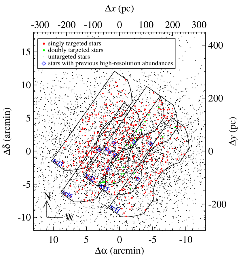
Figure 1.— DEIMOS slitmask footprints laid over a map of sources from the photometric catalog. Targets selected for spectroscopy are shown in red. Targets observed in more than one mask are shown in green. Blue diamonds enclose stars with previous HRS abundance measurements. The left and bottom axis scales show the angular displacement in arcmin from the center of the galaxy ($\alpha_{0}=1^{\rm{h}}00^{\rm{m}}09^{\rm{s}}$, $\delta_{0}=-33^{\circ}42^{\prime}30^{\prime\prime}$, Mateo, 1998), and the right and top axis scales show the physical displacement for an assumed distance of 85.9 kpc (Pietrzyński et al., 2008).

Figure 1 shows the coordinates of all the objects in the catalog regardless of their probability of membership in Sculptor. Five DEIMOS slitmask footprints enclose the spectroscopic targets: scl1, scl2, scl3, scl5, and scl6 (see Tab. 2). The scl5 slitmask included 24 targets also included on other masks. These duplicate observations provide estimates of uncertainty in radial velocity and abundance measurements (Sec. 3.3 and Sec. A.1). The spectral coverage of each slit is not the same. The minimum and maximum wavelengths of spectra of targets near the long, straight edge of the DEIMOS footprint can be up to 400 Å lower than for targets near the irregularly shaped edge of the footprint (upper left and lower right of the slitmask footprints in Fig. 1, respectively). Furthermore, spectra of targets near either extreme of the long axis of the slitmask suffered from vignetting which reduced the spectral range. It is important to keep these differences of spectral range in mind when interpreting the differences of measurements derived from duplicate observations.

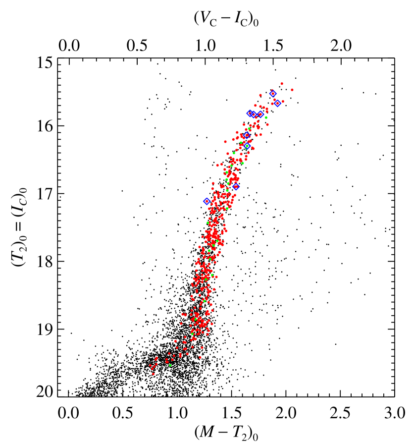
Figure 2.— Color-magnitude diagram in the Washington and Cousins systems for the sources within the right ascension and declination ranges shown in Fig. 1. The symbols have the same meanings as in Fig. 1. The transformation from the Washington system ($M$ and $T_{2}$) to the Cousins system ($V_{\rm C}$ and $I_{\rm C}$) is $I_{\rm C}=T_{2}$ and $V_{\rm C}-I_{\rm C}=0.800(M-T_{2})-0.006$ (Majewski et al., 2000).

Figure 2 shows the color-magnitude diagram (CMD) of the targets within the right ascension and declination ranges of the axes in Fig. 1. The $MT_{2}D$ membership criteria caused the selected red giants to form a tight sequence. This selection may have imposed a metallicity bias on the spectroscopic sample. Although only a tiny fraction of stars lay outside the main locus of the red giant branch, some may have been spectroscopically untargeted members of Sculptor. For example, if Sculptor contained any old stars with ${\rm[Fe/H]}\gtrsim-0.5$, they would have been too red to be included in the spectroscopic sample. Any such metallicity bias should have excluded at most a few stars.

2.3. Spectroscopic Configuration and Exposures

Table 2DEIMOS Observations

Slitmask	Targets	UT Date	Exposures	Seeing
scl1	086	2008 Aug 30	$3\times 1200$ s	$0\farcs 8$
scl2	106	2008 Aug 30	$2\times 900$ s0	$0\farcs 8$
scl3	087	2008 Aug 40	$1\times 462$ s0	$0\farcs 9$
		2008 Aug 31	$1\times 1000$ s	$0\farcs 8$
		2008 Aug 31	$1\times 834$ s0	$0\farcs 8$
scl5	095	2008 Sep 10	$3\times 720$ s0	$0\farcs 8$
scl6	091	2008 Sep 10	$3\times 720$ s0	$1\farcs 2$

Note. — The scl4 slitmask was not observed.

Our observing strategy was nearly identical to that of Simon & Geha (2007) and Kirby et al. (2008a). In summary, we used with the 1200 lines mm^-1 grating at a central wavelength of 7800 Å. The slit widths were $0\farcs 7$, yielding a spectral resolution of $\sim 1.3$ Å FWHM (resolving power $R\sim 6500$ at 8500 Å). The OG550 filter blocked diffraction orders higher than $m=1$. The spectral range was about 6400–9000 Å with variation depending on the slit’s location along the dispersion axis. Exposures of Kr, Ne, Ar, and Xe arc lamps provided wavelength calibration, and exposures of a quartz lamp provided flat fielding. Table 2 lists the number of targets for each slitmask, the dates of observations, the exposure times, and the approximate seeing.

3. Data Reduction

3.1. Extraction of One-Dimensional Spectra

We reduced the raw frames using version 1.1.4 of the DEIMOS data reduction pipeline developed by the DEEP Galaxy Redshift Survey. Guhathakurta et al. (2006) give the details of the data reduction. We also made use of the optimizations to the code described by Simon & Geha (2007, Sec. 2.2 of their article). These modifications provided better extraction of unresolved stellar sources.

In summary, the pipeline traced the edges of slits in the flat field to determine the CCD location of each slit. The wavelength solution was given by a polynomial fit to the CCD pixel locations of arc lamp lines. Each exposure of stellar targets was rectified and then sky-subtracted based on a B-spline model of the night sky emission lines. Next, the exposures were combined with cosmic ray rejection into one two-dimensional spectrum for each slit. Finally, the one-dimensional stellar spectrum was extracted from a small spatial window encompassing the light of the star in the two-dimensional spectrum. The product of the pipeline was a wavelength-calibrated, sky-subtracted, cosmic ray-cleaned, one-dimensional spectrum for each target.

Some of the spectra suffered from unrecoverable defects, such as a failure to find an acceptable polynomial fit to the wavelength solution. There were 53 such spectra. An additional 2 spectra had such poor signal-to-noise ratios (SNR) that abundance measurements were impossible, leaving 410 useful spectra, comprising 393 unique targets and 17 duplicate measurements.

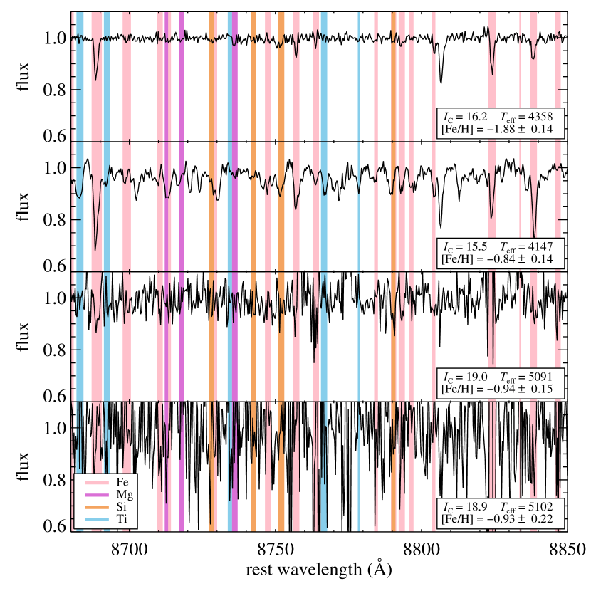
Figure 3.— Examples of small regions of DEIMOS spectra of four different stars. The continuum in each spectrum has been normalized to unity. The $I_{\rm C}$ magnitude, measured effective temperature, and measured [Fe/H] is given for each star. The top two panels show two stars with very different [Fe/H], and the bottom two panels show two stars with nearly the same temperature and [Fe/H] but different SNR. The colors show the regions used to measure each of the Fe, Mg, Si, Ca, and Ti abundances (see Fig. 5).

Figure 3 shows four example spectra at a variety of $I_{\rm C}$ magnitudes, effective temperatures, and [Fe/H]. The two upper panels show stars in the top 10% of the SNR distribution. The two lower panels show stars from the middle and bottom 10% of the distribution.

The one-dimensional DEIMOS spectra needed to be prepared for abundance measurements. The preparation included velocity measurement, removal of telluric absorption, and continuum division. KGS08 (their Sec. 3) described these preparations in detail. We followed the same process with some notable exceptions, described below.

3.2. Telluric Absorption Correction

We removed the absorption introduced into the stellar spectra by the earth’s atmosphere in the same manner as KGS08: division by a hot star template spectrum. However, the high airmass of the Sculptor observations caused much stronger absorption than KGS08 observed in globular cluster (GC) spectra. Even after scaling the hot star template spectrum by the airmass, large residuals in the Sculptor stellar spectra remained. Consequently, we masked spectral regions of heavy telluric absorption before measuring abundances. These regions are 6864–6932 Å, 7162–7320 Å, 7591–7703 Å, 8128–8351 Å, and 8938–10000 Å (see Fig. 5).

3.3. Radial Velocities and Spectroscopic Membership Determination

Our primary interest in this paper is chemical abundances, and we measured radial velocities only to determine membership and to shift the spectra into the rest frame.

Following KGS08, we measured stellar radial velocities by cross-correlation with a template spectrum. However, KGS08 cross-correlated the observed spectra against synthetic spectra whereas we cross-correlated the observed spectra against high SNR template spectra of stars observed with DEIMOS. Templates observed with the same instrument should provide more accurate radial velocity measurements than synthetic templates. Simon & Geha (2007) provided their template spectra to us. For the rest of the analysis, the spectra are shifted to the rest frame.

Figure 4.— Distribution of measured radial velocities for targets in the Sculptor field along with the best-fit Gaussian. The top left label gives the mean and standard deviation of this Gaussian fit. The five stars outside of the dashed lines are not considered Sculptor members. The velocity range of this plot includes all stars for which a velocity measurement was possible.

Although the $MT_{2}D$ selection eliminated almost all of the foreground MW contaminants from the spectroscopic sample, we checked the membership of each target by radial velocity selection. Figure 4 shows the distribution of radial velocities in this spectroscopic data set along with the best-fit Gaussian. We consider the radial velocity limits of Sculptor membership to be $84.8$ km s${}^{-1}<v_{r}<138.3$ km s^-1. We chose these limits because beyond them, the expected number of Sculptor members per 2 km s^-1 bin (the approximate maximum velocity resolution of DEIMOS, Simon & Geha, 2007) is fewer than 0.5. This selection eliminated just 5 out of 393 unique targets.

As a check on our procedure, we compared some derived quantities from the velocity distribution to previous measurements. The mean velocity of our sample is $\langle v_{\rm{helio}}\rangle=111.6\pm 0.5$ km s^-1 with a dispersion of $\sigma_{v}=8.0\pm 0.7$ km s^-1. The velocity dispersion is the per-measurement velocity error subtracted in quadrature from the $1\sigma$ width of the velocity distribution. The per-measurement error is 3.9 km s^-1, which is the standard deviations of the differences in measured velocities for the 17 duplicate spectra. In comparison, Westfall et al. (2006) found $\langle v_{\rm{helio}}\rangle=110.4\pm 0.8$ km s^-1 (difference of $+1.2\sigma$) and $\sigma_{v}=8.8\pm 0.6$ km s^-1 (difference of $-0.9\sigma$). The comparison of the velocity dispersions depends on the assumed binary fraction (Queloz et al., 1995) and—given the presence of multiple kinematically and spatially distinct populations in Sculptor (T04)—the region of spectroscopic selection. Furthermore, Walker et al. (2007, 2009) reported velocity dispersion gradients, and Battaglia et al. (2008a) reported mean velocity gradients along the major axis, indicating rotation. We choose not to address the kinematic complexity of this system in this paper.

3.4. Continuum Determination

In the abundance analysis described in Sec. 4, it is necessary to normalize each stellar spectrum by dividing by the slowly varying stellar continuum. KGS08 determined the continuum by smoothing the regions of the stellar spectrum free from strong absorption lines. Instead of smoothing, we fit a B-spline with a breakpoint spacing of 150 Å to the same “continuum regions” defined by KGS08. Each pixel was weighted by its inverse variance in the fit. Furthermore, the fit was performed iteratively such that pixels that deviated from the fit by more than $5\sigma$ were removed from the next iteration of the fit.

The spline fit results in a smoother continuum determination than smoothing. Whereas the smoothed continuum value may be influenced heavily by one or a few pixels within a relatively small smoothing kernel, the spline fit is a global fit. It is more likely to be representative of the true stellar continuum than a smoothed spectrum.

Shetrone et al. (2009) pointed out the importance of determining the continuum accurately when measuring weak lines in medium-resolution spectra. They refined their continuum determinations by iteratively fitting a high-order spline to the quotient of the observed spectrum and the best-fitting synthetic spectrum. We adopted this procedure as well. As part of the iterative process described in Sec. 4.7, we fit a B-spline with a breakpoint spacing of 50 Å to the observed spectrum divided by the best-fitting synthetic spectrum. We divided the observed spectrum by this spline before the next iteration of abundance measurement.

4. Abundance Measurements

The following section details some improvements on the abundance measurement techniques of KGS08. Aspects of the technique not mentioned here were unchanged from the technique of KGS08. In summary, each observed spectrum was compared to a large grid of synthetic spectra. The atmospheric abundances were adopted from the synthetic spectrum with the lowest $\chi^{2}$.

A major improvement was our measurement of four individual elemental abundances in addition to Fe: Mg, Si, Ca, and Ti. We chose these elements because they are important in characterizing the star formation history of a stellar population and because a significant number of lines represent each of them in the DEIMOS spectral range.

4.1. Model Atmospheres

Like KGS08, we built synthetic spectra based on ATLAS9 model atmospheres (Kurucz, 1993) with no convective overshooting (Castelli et al., 1997). KGS08 chose to allow the atmospheres to have ${\rm[\alpha/Fe]}=+0.4$ or ${\rm[\alpha/Fe]}=0.0$. This choice allowed them to use the large grid of ATLAS9 model atmospheres computed with new opacity distribution functions (Castelli & Kurucz, 2004). However, we found that best-fitting model spectra computed by KGS08 tended to cluster around ${\rm[\alpha/Fe]}=+0.2$ due to the discontinuity in $\chi^{2}$ caused by the abrupt switch between alpha-enhanced and solar-scaled models.

Table 3New Grid of ATLAS9 Model Atmospheres

Parameter	Minimum Value	Maximum Value	Step
$T_{\rm{eff}}$ (K)	3500	5600	100
	5600	8000	200
$\log g$ (cm s-2)	0.0 ($T_{\rm eff}<7000$ K)	5.0	0.5
	0.5 ($T_{\rm eff}\geq 7000$ K)	5.0	0.5
[A/H]	$-4.0$	$0.0$	$0.5$
[$\alpha$/Fe]	$-0.8$	$+1.2$	$0.1$

To avoid this discontinuity, we recomputed ATLAS9 model atmospheres on the grid summarized in Table 3. The new grid required recomputing new opacity distribution functions (ODFs), for which we used the DFSYNTHE code (Castelli, 2005). Unlike the grid of Castelli & Kurucz (2004), we adopted the solar composition of Anders & Grevesse (1989), except for Fe, for which we followed Sneden et al. (1992, see the note in Table 4). One opacity distribution function was computed for each of the 189 combinations of [A/H] and [$\alpha$/Fe] specified in Table 3. The abundances of all the elements except H and He were augmented by [A/H]. Additionally, the abundances of O, Ne, Mg, Si, Ar, Ca, and Ti were augmented by [$\alpha$/Fe]. These ODFs were used to compute one ATLAS9 model atmosphere for each grid point in Table 3 and for two values of microturbulent velocity, for a total of 139104 model atmospheres.

4.2. Microturbulent Velocity

In order to reduce the number of parameters required to determine a stellar abundance, KGS08 assumed that the microturbulent velocity ($\xi$) of the stellar atmosphere was tied to the surface gravity ($\log g$). They chose to fit a line to the spectroscopically measured $\xi$ and $\log g$ of the giant stars in Fulbright’s (2000) sample:

$$\xi~{}(\mathrm{km~{}s}^{-1})=2.70-0.51\,\log g$$ (1)

We also adopted a relation between $\xi$ and $\log g$, but we re-determined this relation from the GC red giant sample of KGS08 combined with Kirby’s (2009) compilation of high-resolution spectroscopic measurements from the literature (Frebel et al., 2009; Geisler et al., 2005; Johnson, 2002; Lai et al., 2007; Shetrone et al., 2001, 2003, and references from KGS08). The best-fit line between the spectroscopically measured $\xi$ and $\log g$ is

$$\xi~{}(\mathrm{km~{}s}^{-1})=(2.13\pm 0.05)-(0.23\pm 0.03)\,\log g\>.$$ (2)

corresponding roughly to a 0.0–0.5 km s^-1 decrease in $\xi$, depending on $\log g$. In the generation of the grid of synthetic stellar spectra described in Sec. 4.4, $\xi$ was not a free parameter, but was fixed to $\log g$ via Eq. 2.

In general, a decrease in $\xi$ increases the measurement of [Fe/H]. Therefore, this change tended to increase the derived values of [Fe/H]. A typical change in [Fe/H] was $\lesssim+0.05$ dex. This change would be more severe in an HRS analysis based on equivalent widths (EWs). In our $\chi^{2}$ minimization, the abundance measurement was most sensitive to lines with large $d({\rm EW})/d{\rm[Fe/H]}$. Such lines are the weak, unsaturated transitions whose strength does not depend on $\xi$. The DEIMOS spectra contain enough of these weak lines that $\xi$ did not play a large role in the abundance determination.

4.3. Line List

We compared the Fe I oscillator strengths ($\log gf$) in the KGS08 line list to values measured in the laboratory (Fuhr & Wiese, 2006). Most of the KGS08 oscillator strengths were stronger than the laboratory measurements. The average offset was 0.13 dex. Because KGS08 calibrated their line list to the solar spectrum, we interpreted this offset as a systematic error in the solar model atmosphere, solar spectral synthesis, and/or solar composition. Accepting the laboratory-measured values as more accurate than the solar calibration, we replaced Fe I oscillator strengths with Fuhr & Wiese where available, and we subtracted 0.13 dex from $\log gf$ for all other Fe I transitions in the KGS08 line list. All other data remained unchanged.

Decreasing the oscillator strengths requires a larger [Fe/H] to match the observed spectrum. The amount of change in [Fe/H] depends on the atmospheric parameters as well as the saturation of the measured Fe lines. From comparison of results with the old and new line lists, we estimate a typical change in [Fe/H] to be $\sim+0.1$ dex.

4.4. Generation of Synthetic Spectra

The spectra were synthesized as described in KGS08. Specifically, the current version of the local thermodynamic equilibrium (LTE) spectrum synthesis software MOOG (Sneden, 1973) generated one spectrum for each point on the grid. The spectral grid was more finely spaced in [Fe/H] than the model atmosphere grid. The spacing is 0.1 dex for each of [Fe/H] and [$\alpha$/Fe], yielding a total of 316848 synthetic spectra.

Table 4Adopted Solar Composition

Element	$12+\log\epsilon$	Element	$12+\log\epsilon$
Mg	7.58	Ti	4.99
Ca	6.36	Fe	7.52
Si	7.55

Note. — This composition is adopted from Anders & Grevesse (1989), except for Fe. For justification of the adopted Fe solar abundance, see Sneden et al. (1992). The abundance of an element X is defined as its number density relative to hydrogen: $12+\log\epsilon_{\rm{X}}=12+\log(n_{\rm{X}})-\log(n_{\rm{H}})$.

The solar composition used in the generation of the synthetic spectra was identical to the solar composition used in the computation of the model atmospheres. Table 4 lists the adopted solar abundances for the five elements for which we measure abundances in Sculptor stars.

4.5. Effective Temperatures and Surface Gravities

Different spectroscopic studies of chemical abundances rely on different sources of information for determining the effective temperature ($T_{\rm{eff}}$) and surface gravity ($\log g$) of the stellar atmosphere. KGS08 consulted Yonsei-Yale model isochrones (Demarque et al., 2004) to determine the temperature and gravity that correspond to a dereddened color and an extinction-corrected absolute magnitude. They also considered Victoria-Regina (VandenBerg et al., 2006) and Padova (Girardi et al., 2002) model isochrones, as well as an empirical color-temperature relation (Ramírez & Meléndez, 2005).

The Fe lines accessible in DEIMOS spectra span a large range of excitation potential. Together, these different lines provide a constraint on $T_{\rm{eff}}$. KGS08 (their Sec. 5.1) showed that—without any photometric information—the synthesis analysis of medium-resolution spectra of GC stars yielded values of $T_{\rm{eff}}$ very close to values previously measured from HRS. Therefore, we chose to measure $T_{\rm{eff}}$ from photometry and spectroscopy simultaneously.

To begin, we converted extinction-corrected (Schlegel et al., 1998) Washington $M$ and $T_{2}$ magnitudes to Cousins $V_{\rm C}$ and $I_{\rm C}$ magnitudes (Majewski et al., 2000). With these magnitudes, we computed $T_{\rm{eff}}$ from the Yonsei-Yale, Victoria-Regina, and Padova model isochrones, as well as the Ramírez & Meléndez (2005) empirical color-based $T_{\rm{eff}}$. For each measurement, we estimated the effect of photometric error by measuring the standard deviation of $T_{\rm{eff}}$ determined from 1000 Monte Carlo realizations of $V_{\rm C}$ and $I_{\rm C}$. In each realization, $V_{\rm C}$ and $I_{\rm C}$ were chosen from a normal distribution with a mean of the measured, extinction-corrected magnitude and a standard deviation of the photometric error. We call this error $\delta T_{{\rm eff,}i}$, where $i$ represents each of the four photometric methods of determining $T_{\rm{eff}}$. In order to arrive at a single photometric $T_{\rm{eff}}$, we averaged the four $T_{{\rm eff,}i}$ together with appropriate error weighting. We also estimated the random and systematic components of error. In summary,

$$\overline{T_{\rm{eff}}} = \frac{\sum_{i}T_{{\rm eff,}i}\delta T_{{\rm eff,}i}^{-2}}{\sum_{i}\delta T_{{\rm eff,}i}^{-2}}$$ (3)

$$\delta_{\rm{rand}}T_{\rm{eff}} = \frac{\sum_{i}\delta T_{{\rm eff,}i}^{-1}}{\sum_{i}\delta T_{{\rm eff,}i}^{-2}}$$ (4)

$$\delta_{\rm{sys}}T_{\rm{eff}} = \sqrt{\frac{\sum_{i}\delta T_{{\rm eff,}i}^{-2}\sum_{i}\delta T_{{\rm eff,}i}^{-2}\left(T_{{\rm eff,}i}-\overline{T_{\rm{eff}}}\right)^{2}}{1-\left(\sum_{i}\delta T_{{\rm eff,}i}^{-2}\right)^{2}\sum_{i}\delta T_{{\rm eff,}i}^{-4}}}$$ (5)

$$\delta_{\rm{total}}T_{\rm{eff}} = \sqrt{(\delta_{\rm{rand}}T_{\rm{eff}})^{2}+(\delta_{\rm{sys}}T_{\rm{eff}})^{2}}$$ (6)

For the stars in this data set, the median random, systematic, and total errors on $T_{\rm{eff}}$ were 98 K, 58 K, and 117 K respectively. The somewhat large errors on the photometric temperatures indicated that the spectra may help constrain $T_{\rm{eff}}$. Therefore, Eq. 3 does not show the final temperature used in the abundance determination. Section 4.7 describes the iterative process for determining $T_{\rm{eff}}$ and elemental abundances from spectroscopy.

We followed a similar procedure for determining $\log g$ photometrically, except that we used only the three model isochrones and not any empirical calibration. The error on the true distance modulus ($19.67\pm 0.12$, Pietrzyński et al., 2008) was included in the Monte Carlo determination of the error on $\log g$. The median random, systematic, and total errors on $\log g$ were 0.06, 0.01, and 0.06. These errors are very small, and the medium-resolution, red spectra have little power to help constrain $\log g$ because there are so few ionized lines visible. Therefore, we assumed the photometric value of $\log g$ for the abundance analysis.

4.6. Wavelength Masks

The procedure described in the next section consisted of separately measuring the abundances of five elements: Mg, Si, Ca, Ti, and Fe. The procedure relied on finding the synthetic spectrum that best matched an observed spectrum. In order to make this matching most sensitive to a particular element, we masked all spectral regions that were not significantly affected by abundance changes of that element.

To make the wavelength masks, we began with a base spectrum that represented the solar composition in which the abundances of all the metals were scaled down by 1.5 dex ($\rm{[A/H]}=-1.5$). The temperature and gravity of the synthetic star were $T_{\rm eff}=4000$ K and $\log g=1.0$. Then, we created two pairs of spectra for each of the five elements. In one spectrum, the abundance of the element was enhanced by 0.3 dex, and in the other, depleted by 0.3 dex. Spectral regions where the flux difference between these two spectra exceeds 0.5% were used in the abundance determination of that element. This small threshold assured that weak lines, which experience large fractional changes in EW as [Fe/H] changes, were included in the analysis. We repeated this procedure for spectra with $T_{\rm eff}=5000$ K, 6000 K, 7000 K, and 8000 K. Additional spectral regions that passed the 0.5% flux difference criterion were also included in the abundance determination of that element. All other wavelengths were masked.

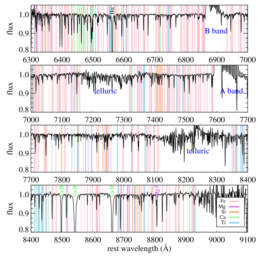
Figure 5.— A coaddition of all Sculptor stars with the continuum normalized to unity. The high SNR provided by the coaddition makes stellar absorption lines readily apparent. The colored regions show the wavelength masks used in the determination of the abundance of each element. Regions susceptible to telluric absorption are labeled with blue text. Because large residuals from the telluric absorption correction remain, we eliminate these regions from the abundance analysis. Some stellar features excluded from the abundances measurement are also labeled.

The result was one wavelength mask for each of Mg, Si, Ca, Ti, and Fe, shown in Fig. 5. We also created one “$\alpha$” mask as the intersection of the Mg, Si, Ca, and Ti masks. The $\alpha$ element regions do not overlap with each other, but the $\alpha$ element regions do overlap with the Fe regions. The most severe case is the Ca mask, where $\sim 35\%$ of the pixels are shared with the Fe mask. However, the overlap did not introduce interdependence in the abundance measurements. The $\alpha$ element abundances were held fixed while [Fe/H] was measured, and the Fe abundance was held fixed while [$\alpha$/Fe] was measured. The measurements of [Fe/H] and [$\alpha$/Fe] were performed iteratively (see the next subsection). We tested the independence of the measurements by removing all overlapping pixels from consideration. Abundance measurements changed on average by only 0.01 dex.

4.7. Measuring Atmospheric Parameters and Elemental Abundances

A Levenberg-Marquardt algorithm (the IDL routine MPFIT, written by Markwardt, 2009) found the best-fitting synthetic spectrum in ten iterative steps. In each step, the $\chi^{2}$ was computed between an observed spectrum and a synthetic spectrum degraded to match the resolution of the observed spectrum. First, we interpolated the synthetic spectrum onto the same wavelength array as the observed spectrum. Then, we smoothed the synthetic spectrum through a Gaussian filter whose width was the observed spectrum’s measured resolution as a function of wavelength.

1. $T_{\rm{eff}}$ and [Fe/H], first pass: An observed spectrum was compared to a synthetic spectrum with $T_{\rm{eff}}$ and $\log g$ determined as described in Sec. 4.5 and [Fe/H] determined from Yonsei-Yale isochrones. For this iteration, [$\alpha$/Fe] was fixed at 0.0 (solar), and only spectral regions most susceptible to Fe absorption (Sec. 4.6) were considered. The two quantities $T_{\rm{eff}}$ and [Fe/H] were varied, and the algorithm found the best-fitting synthetic spectrum by minimizing $\chi^{2}$. We sampled the parameter space between grid points by linearly interpolating the synthetic spectra at the neighboring grid points. $T_{\rm{eff}}$ was also loosely constrained by photometry. As the spectrum caused $T_{\rm{eff}}$ to stray from the photometric values, $\chi^{2}$ increased, and it increased more sharply for smaller photometric errors (as calculated in Eq. 6). Therefore, both photometry and spectroscopy determined $T_{\rm{eff}}$. Photometry alone determined $\log g$.

2. [$\alpha$/Fe], first pass: For this iteration, $T_{\rm{eff}}$, $\log g$, and [Fe/H] were fixed. Only [$\alpha$/Fe] was allowed to vary. In the model stellar atmosphere, the abundances of the $\alpha$ elements with respect to Fe varied together. Only the spectral regions susceptible to absorption by Mg, Si, Ca, or Ti were considered.

3. Continuum refinement: The continuum-divided, observed spectrum was divided by the synthetic spectrum with the parameters determined in steps 1 and 2. The result approximated a flat noise spectrum. To better determine the continuum, we fit a B-spline with a breakpoint spacing of 50 Å to the residual spectrum. We divided the observed spectrum by the spline fit.

4. [Fe/H], second pass: We repeated step 1 with the revised spectrum, but $T_{\rm{eff}}$ was held fixed at the previously determined value.

5. [Mg/Fe]: We repeated step 2. However, only Mg spectral lines were considered in the abundance measurement.

6. [Si/Fe]: We repeated step 5 for Si instead of Mg.

7. [Ca/Fe]: We repeated step 5 for Ca instead of Mg.

8. [Ti/Fe]: We repeated step 5 for Ti instead of Mg.

9. [$\alpha$/Fe], second pass: We repeated step 2 for all of the $\alpha$ elements instead of just Mg. This step was simply a different way to average the $\alpha$ element abundances than combining the individual measurements of [Mg/Fe], [Si/Fe], [Ca/Fe], and [Ti/Fe].

10. [Fe/H], third pass: The value of [$\alpha$/Fe] affected the measurement of [Fe/H] because [$\alpha$/Fe] can affect the structure of the stellar atmosphere. Specifically, the greater availability of electron donors with an increased [$\alpha$/Fe] ratio allows for a higher density of H^- ions. The subsequent increase in continuous opacity decreases the strength of Fe and other non-$\alpha$ element lines. With [$\alpha$/Fe] fixed at the value determined in step 9, we re-measured [Fe/H]. Typically, [Fe/H] changed from the value determined in step 1 by much less than 0.1 dex.

4.8. Correction to [Fe/H]

In comparing our MRS measurements of [Fe/H] to HRS measurements of the same stars (see the appendix), we noticed that our measurements of metal-poor stars were consistently $\sim 0.15$ dex lower. The same pattern is also visible in the Kirby et al. (2008a) GC measurements (see their Figs. 6, 7, 10, and 11).

We have thoroughly examined possible sources of this difference of scale. The changes to the microturbulent velocity relation (Sec. 4.2) and the line list (Sec. 4.3) were intended to yield a more accurate and standardized estimation of [Fe/H], but the offset still remained. Restricting the analysis to narrow spectral regions did not reveal any systematic trend of [Fe/H] with wavelength.

A possible explanation for this offset is overionization (Thévenin & Idiart, 1999). Ultraviolet radiation in stellar atmospheres can ionize Fe more than would be expected in LTE. Therefore, the abundance of Fe I would seem to be lower than the abundance of Fe II in an LTE analysis. Fe II does not suffer from this effect. However, the effect is smaller at higher [Fe/H], and we do not observe a trend with metallicity for the offset of our values relative to HRS studies.

In order to standardize our measurements with previous HRS studies, we added 0.15 dex to all of our measurements of [Fe/H]. This offset and the microturbulent velocity-surface gravity relation are the only ways in which previous HRS studies inform our measurements. Furthermore, this offset is not intended to change the standardization of our abundances. All of the abundance in this article, including those from other studies, are given relative to the solar abundances quoted in Table 4.

4.9. Error Estimation

Table 5Systematic Abundance Errors

Element Ratio	$\delta_{\rm sys}$	Element Ratio	$\delta_{\rm sys}$
[Fe/H]	0.136	[Ca/Fe]	0.087
[Mg/Fe]	0.108	[Ti/Fe]	0.101
[Si/Fe]	0.179

We repeated the error estimation procedure described by KGS08 (their Sec. 6) by repeating their abundance analysis on GC stars with the above modifications. We no longer found a convincing trend of $\delta{\rm[Fe/H]}$ with [Fe/H]. Instead, we estimate the total error on [Fe/H] by adding a systematic error in quadrature with the SNR-dependent uncertainty of the synthetic spectral fit. The magnitude of $\delta_{\rm{sys}}{\rm[Fe/H]}=0.136$ was the value required to force HRS and MRS [Fe/H] estimates of the same GC stars to agree at the 1$\sigma$ level. We also estimated systematic errors for each of [Mg/Fe], [Si/Fe], [Ca/Fe], and [Ti/Fe] in the same manner as for [Fe/H]. These are listed in Table 5.

5. Results

In this section, we discuss the interpretation of the abundance measurements in Sculptor, all of which are presented in Table 6 on the last page of this manuscript.

5.1. Metallicity Distribution

The metallicity distribution function (MDF) of a dwarf galaxy can reveal much about its star formation history. In chemical evolution models of dwarf galaxies (e.g., Lanfranchi & Matteucci, 2004; Marcolini et al., 2006, 2008), the duration of star formation affects the shape of the MDF. The MDF also has implications for the formation of the MW. If the MW halo was built from dSphs (Searle & Zinn, 1978; White & Rees, 1978), then it is important to find dSph counterparts to halo field stars at all metallicities, as pointed out by Helmi et al. (2006, hereafter H06).

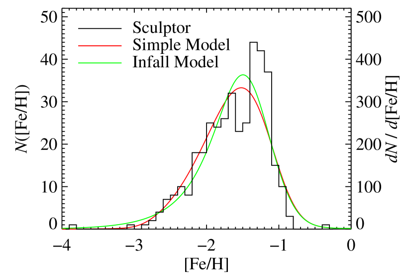
Figure 6.— The metallicity distribution in Sculptor. The red curve is the maximum likelihood fit to a galactic chemical evolution model with pre-enrichment (Eq. 7), and the green curve is the maximum likelihood fit to a model of star formation in the presence of infalling, zero-metallicity gas (Eq. 5.1.2). The long, metal-poor tail is typical for systems with non-instantaneous star formation.

Figure 6 shows the MDF of Sculptor. The shape of the MDF is highly asymmetric, with a long, metal-poor tail (as predicted by Salvadori & Ferrara, 2009). The inverse-variance weighted mean is $\langle{\rm[Fe/H]}\rangle=-1.58$ with a standard deviation of $0.41$. The median is $-1.58$ with a median absolute deviation of $0.33$ and an interquartile range of $0.67$.

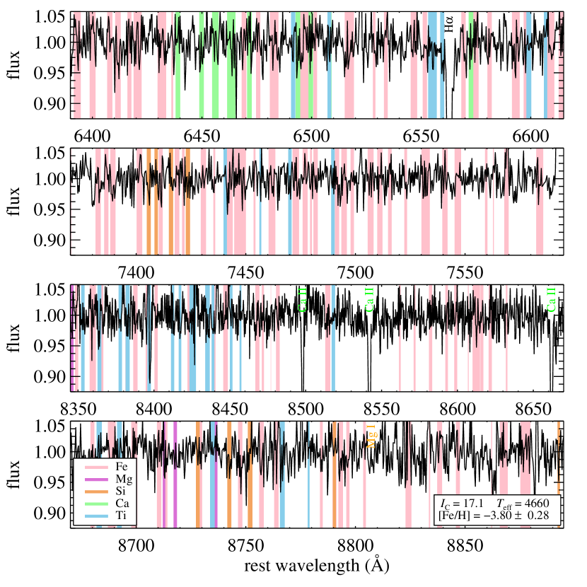
Figure 7.— Regions of the DEIMOS spectrum of the extremely metal-poor star S1020549, which has ${\rm[Fe/H]}=-3.80\pm 0.28$. The spectrum appears particularly noisy because the $y$-axis range is small. Some Fe absorption lines are barely detectable, but all together, they contain enough signal to make a quantitative measurement of [Fe/H]. The shading corresponds to the same spectral region shown in Fig. 5. Frebel, Kirby, & Simon (in preparation) will present a high-resolution spectrum of this star, which confirms the extremely low metallicity.

The MDF boasts an exceptionally metal-poor star, S1020549. The metallicity is ${\rm[Fe/H]}=-3.80\pm 0.28$. Figure 7 shows how weak the Fe absorption lines are in this star. Frebel, Kirby, & Simon (in preparation) have confirmed this extremely low metallicity with a high-resolution spectrum.

Sculptor is now the most luminous dSph in which an extremely metal-poor (EMP, ${\rm[Fe/H]}<-3$) star has been detected. [Kirby et al. (2008b) discovered 15 EMP stars across eight ultra-faint dwarf galaxies, and Cohen & Huang (2009) discovered one EMP star in the Draco dSph (catalog NAME DRACO DSPH GALAXY).] Stars more metal-poor than S1020549 are known to exist only in the field of the Milky Way field. This discovery hints that dSph galaxies like Sculptor may have contributed to the formation of the metal-poor component of the halo. We discuss Sculptor’s link to the halo further in Sec. 5.1.3.

The $MT_{2}D$ photometric selection of spectroscopic targets may have introduced a tiny [Fe/H] bias. Figure 2 shows that the RGB is sharply defined in Sculptor. Because the number density of stars redward and blueward of the RGB is much lower than the number density on the RGB, the number of very young or very metal-poor stars (blueward) or very metal-rich stars (redward) missed by photometric pre-selection must be negligible. Furthermore, the hard color cut (as opposed to one that depends on $M-D$ color) was $0.6<(M-T_{2})_{0}<2.2$. The CMD gives no reason to suspect Sculptor RGB members outside of these limits, but it is possible that some extremely blue Sculptor members have been excluded.

5.1.1 Possible Explanation of the Discrepancy with Previous Results

Our measured MDF and our detection of EMP stars in Sculptor are at odds with the findings of H06. Whereas our MDF peaks at ${\rm[Fe/H]}\sim-1.3$, theirs peaks at ${\rm[Fe/H]}\sim-1.8$. Furthermore, our observed MDF is much more asymmetric than that of H06, which may even be slightly asymmetric in the opposite sense (a longer metal-rich tail). The greater symmetry would indicate a less extended star formation history or early infall of a large amount of gas (Prantzos, 2003).

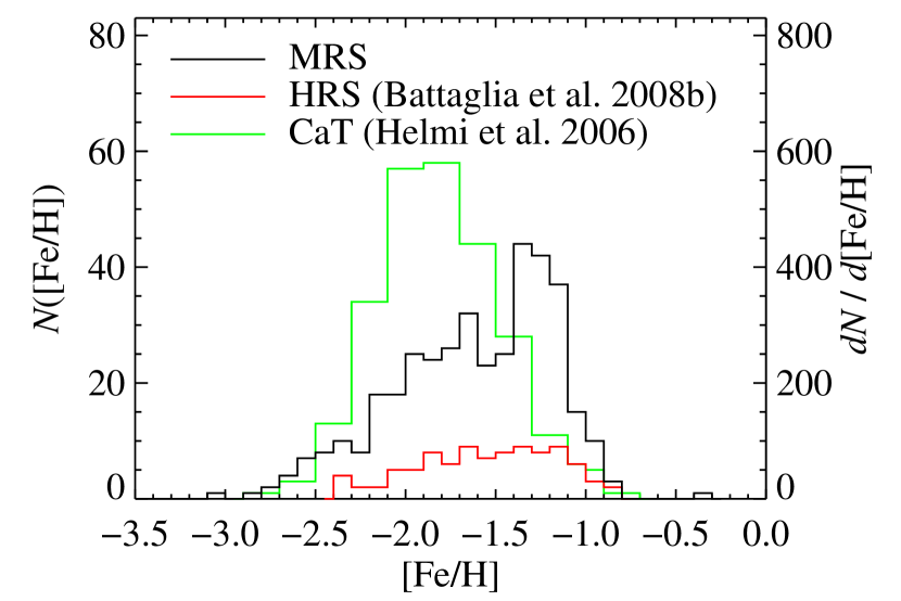
Figure 8.— Sculptor’s metallicity distribution as observed in this study (MRS, black) and by B08b (HRS, red), which is a subset of the MDF observed by H06 (Ca triplet, green). The CaT-based MDF is more metal-poor probably because the sample of H06 is more spatially extended than the other two samples.

Battaglia et al. (2008b, hereafter B08b) observed a subset of the H06 stars at high resolution. The MDFs from the two studies have noticeably different shapes. Figure 8 shows that the HRS MDF peaks at ${\rm[Fe/H]}\sim-1.3$, which is also the peak that we observe. The mean and standard deviation of their MDF are $-1.56$ and $0.38$. However, the MDF of H06 peaks at ${\rm[Fe/H]}\sim-1.8$, and the mean and standard deviation are $-1.82$ and $0.35$. The overlapping stars between the samples of B08b and H06 agree very well.

The most likely explanation for the different MDFs is the different spatial sampling of the three studies. Sculptor has a steep radial metallicity gradient (Tolstoy et al., 2004; Westfall et al., 2006; Walker et al., 2009, also see Sec. 5.3). The stars in the center of Sculptor are more metal-rich than stars far from the center. H06 sampled stars out to the tidal radius ($r_{t}=76.5$ arcmin, Mateo, 1998), but we and B08b sampled stars only out to about 11 arcmin. As a result, the mean metallicity of the H06 CaT sample is lower than our MRS sample and the B08b HRS sample. In the next subsection, we address the chemical evolution of Sculptor based on its MDF. Our conclusions are based only on stars within the central 11 arcmin.

5.1.2 Quantifying Chemical Evolution in Sculptor

In chemical evolution models, extended star formation produces a long, metal-poor tail. Prantzos (2008) described the shape of the differential metallicity distribution derived from a “simple model” of galactic chemical evolution. Expressed in terms of [Fe/H] instead of metal fraction $Z$, the predicted distribution is

$$\frac{dN}{d{\rm[Fe/H]}}=A\left(10^{{\rm[Fe/H]}}-10^{{\rm[Fe/H]}_{i}}\right)\exp\left(-\frac{10^{{\rm[Fe/H]}}}{p}\right)$$ (7)

where $p$ is the effective yield in units of the solar metal fraction ($Z_{\sun}$) and ${\rm[Fe/H]}_{i}$ is the initial gas metallicity. An initial metallicity is needed to resolve the Galactic G dwarf problem (van den Bergh, 1962; Schmidt, 1963). $A$ is a normalization that depends on $p$, ${\rm[Fe/H]}_{i}$, the final metallicity ${\rm[Fe/H]}_{f}$, and the number of stars in the sample $N$:

$$A=\frac{(N\ln 10)/p}{\exp\left(-\frac{10^{{\rm[Fe/H]}_{i}}}{p}\right)-\exp\left(-\frac{10^{{\rm[Fe/H]}_{f}}}{p}\right)}$$ (8)

The red curve in Figure 6 is the two-parameter, maximum likelihood fit to Eq. 7. The likelihood $L_{i}$ that star $i$ is drawn from the probability distribution defined by Eq. 7 is the integral of the product of the error distribution for the star and the probability distribution. The total likelihood $L=\prod_{i}L_{i}$. The most likely $p$ and ${\rm[Fe/H]}_{0}$ are the values that maximize $L$. For display, the curve has been convolved with an error distribution, which is a composite of $N$ unit Gaussians. $N$ is the total number of stars in the observed distribution, and the width of the $i^{\rm th}$ Gaussian is the estimated total [Fe/H] error on the $i^{\rm th}$ star. This convolution approximates the effect of measurement error on the model curve under the assumption that the error on [Fe/H] does not depend on [Fe/H]. This assumption seems to be valid because our estimates of $\delta{\rm[Fe/H]}$ do not show a trend with [Fe/H].

The most likely yield—largely determined by the [Fe/H] at the peak of the MDF—is $p=0.031Z_{\sun}$. [From the MDF of H06, Prantzos (2008) calculated $p=0.016Z_{\sun}$.] We also measure ${\rm[Fe/H]}_{0}=-2.92$. H06 also measured ${\rm[Fe/H]}_{0}=-2.90\pm 0.21$ for Sculptor, even though they included stars out to the tidal radius, which are more metal-poor on average than the centrally concentrated stars in our sample. (Instead of finding the maximum likelihood model, they performed a least-squares fit to the cumulative metallicity distribution without accounting for experimental uncertainty. In general, observational errors exaggerate the extrema of the metallicity distribution, and the least-squares fit converges on a lower ${\rm[Fe/H]}_{0}$ than the maximum likelihood fit.) One explanation that they proposed for this non-zero initial metallicity was pre-enrichment of the interstellar gas that formed the first stars. Pre-enrichment could result from a relatively late epoch of formation for Sculptor, after the supernova (SN) ejecta from other galaxies enriched the intergalactic medium from which Sculptor formed. However, our observation of a star at ${\rm[Fe/H]}=-3.80$ is inconsistent with pre-enrichment at the level of ${\rm[Fe/H]}_{0}=-2.9$.

Prantzos (2008) instead interpreted the apparent dearth of EMP stars as an indication of early gas infall (Prantzos, 2003), wherein star formation begins from a small amount of gas while the majority of gas that will eventually form dSph stars is still falling in. In order to test this alternative to pre-enrichment, we have also fit an Infall Model, the “Best Accretion Model” of Lynden-Bell (1975, also see ). It is one of the models which accounts for a time-decaying gas infall that has an analytic solution. The model assumes that the gas mass $g$ in units of the initial mass is related quadratically to the stellar mass $s$ in units of the initial mass:

$$g(s)=\left(1-\frac{s}{M}\right)\left(1+s-\frac{s}{M}\right)$$ (9)

where $M$ is a parameter greater than 1. When $M=1$, Eq. 9 reduces to $g=1-s$, which describes the Closed Box Model. Otherwise, $M$ monotonically increases with the amount of gas infall and with the departure from the Simple Model. Following Lynden-Bell (1975) and Pagel (1997), we assume that the initial and infalling gas metallicity is zero. The differential metallicity distribution is described by two equations.

$${\rm[Fe/H]}(s) = \log\Big{\{}p\left(\frac{M}{1+s-\frac{s}{M}}\right)^{2}\times$$

$$\left[\ln\frac{1}{1-\frac{s}{M}}-\frac{s}{M}\left(1-\frac{1}{M}\right)\right]\Big{\}}$$

$$\frac{dN}{d{\rm[Fe/H]}} = A\frac{10^{{\rm[Fe/H]}}}{p}\times$$

$$\frac{1+s\left(1-\frac{1}{M}\right)}{\left(1-\frac{s}{M}\right)^{-1}-2\left(1-\frac{1}{M}\right)\times 10^{{\rm[Fe/H]}/p}}$$

Equation 5.1.2 is transcendental, and it must be solved for $s$ numerically. Equation 5.1.2 decouples the peak of the MDF from the yield $p$. As $M$ increases, the MDF peak decreases independently of $p$.

The green line in Fig. 6 shows the most likely Infall Model convolved with the error distribution as described above. The Infall Model has $M=1.76$, which is only a small departure from the Simple Model.

Neither the Simple Model nor the Infall Model fits the data particularly well. Both models fail to reproduce the sharp peak at ${\rm[Fe/H]}\sim-1.3$ and the steep metal-rich tail. However, the Infall Model does reproduce the metal-poor tail about as well as the Simple Model. Therefore, the Infall Model is a reasonable alternative to pre-enrichment, and it allows the existence of the star at ${\rm[Fe/H]}=-3.80$. In reality, a precise explanation of the MDF will likely incorporate the radial metallicity gradients and multiple, superposed populations. It is tempting to conclude from Fig. 6 that Sculptor displays two metallicity populations. We have not attempted a two-component fit, but that would seem to be a reasonable approach for future work, especially in light of Tolstoy et al.’s (2004) report of two distinct stellar populations in Sculptor.

Searches for the lowest metallicity stars in the MW halo have revealed some exquisitely metal-poor stars (e.g., ${\rm[Fe/H]}=-5.96$, Frebel et al., 2008). Such exotic stars have not yet been discovered in any dSph. However, if Sculptor was not pre-enriched, a large enough sample of [Fe/H] measurements in Sculptor—and possibly other dSphs—may reveal stars as metal-poor as the lowest metallicity stars in the MW halo.

5.1.3 Comparison to the Milky Way Halo MDF

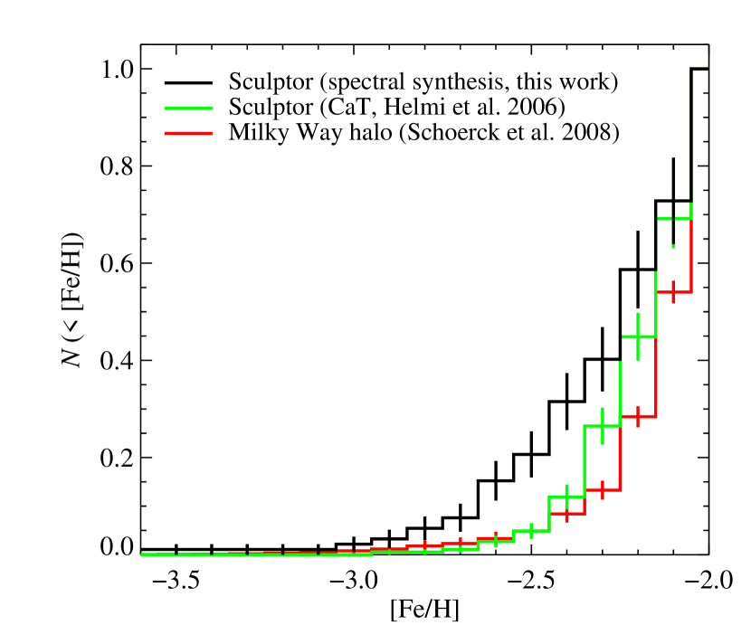
Figure 9.— The metal-poor tails of the MDFs in Sculptor (black) and Galactic halo field stars (red, Schoerck et al., 2008) shown as cumulative distributions, all normalized to the number of stars with ${\rm[Fe/H]}<-2$. The green line shows the MDF measured by the DART team (Helmi et al., 2006) with a calibration based on the Ca triplet. The calibration may overpredict very low metallicities. The synthesis-based metallicities (black, this work) are valid at lower [Fe/H] than the Ca triplet [Fe/H]. Regardless, the halo has a steeper metal-poor tail than Sculptor in both representations. Galaxies such as Sculptor were probably not the dominant contributors to the halo.

Searle & Zinn (1978) and White & Rees (1978) posited that the MW halo formed from the accretion and dissolution of dwarf galaxies. The dSphs that exist today may be the survivors from the cannibalistic construction of the Galactic halo. Helmi et al. (2006) suggested that at least some of the halo field stars could not have come from counterparts to the surviving dSphs because the halo field contained extremely metal-poor stars whereas the dSphs do not. However, Schoerck et al. (2008) showed that the Hamburg/ESO Survey’s halo MDF, after correction for selection bias, actually looks remarkably like the MDFs of the dSphs Fornax, Ursa Minor (catalog NAME UMi dSph), and Draco. Furthermore, Kirby et al. (2008b) presented MRS evidence for a large fraction of EMP stars in the ultra-faint dSph sample of Simon & Geha (2007), suggesting that today’s surviving dSphs contain stars that span the full range of metallicities displayed by the Galactic field halo population.

We revisit the halo comparison with the present MDF for Sculptor. Figure 9 shows the metal-poor tail (${\rm[Fe/H]}<-2$) of the MRS synthesis-based Sculptor MDF presented here, the CaT-based Sculptor MDF (Helmi et al., 2006), and the MW halo MDF (Schoerck et al., 2008). As observed in the comparisons to other dSphs presented by Schoerck et al., the halo seems to have a steeper metal-poor tail than the CaT-based Sculptor MDF, despite the evidence that CaT-based metallicities overpredict [Fe/H] at ${\rm[Fe/H]}\lesssim-2.2$ (e.g., Koch et al., 2008; Norris et al., 2008). The synthesis-based MDF does not rely on empirical calibrations, and the technique has been shown to work at least down to ${\rm[Fe/H]}=-3$ (Kirby et al., 2008b).

This MDF shows that the halo has a much steeper metal-poor tail than Sculptor. This result is consistent with a merging scenario wherein several dwarf galaxies significantly larger than Sculptor contributed most of the stars to the halo field (e.g., Robertson et al., 2005; Font et al., 2006). In these models, the more luminous galaxies have higher mean metallicities. Galaxies with a Sculptor-like stellar mass are minority contributors to the halo field star population. Less luminous galaxies are even more metal-poor (Kirby et al., 2008b). Therefore, Sculptor conforms to the luminosity-metallicity relation for dSphs, and the difference between Sculptor’s MDF and the MW halo MDF does not pose a problem for hierarchical assembly.

5.2. Alpha Element Abundances

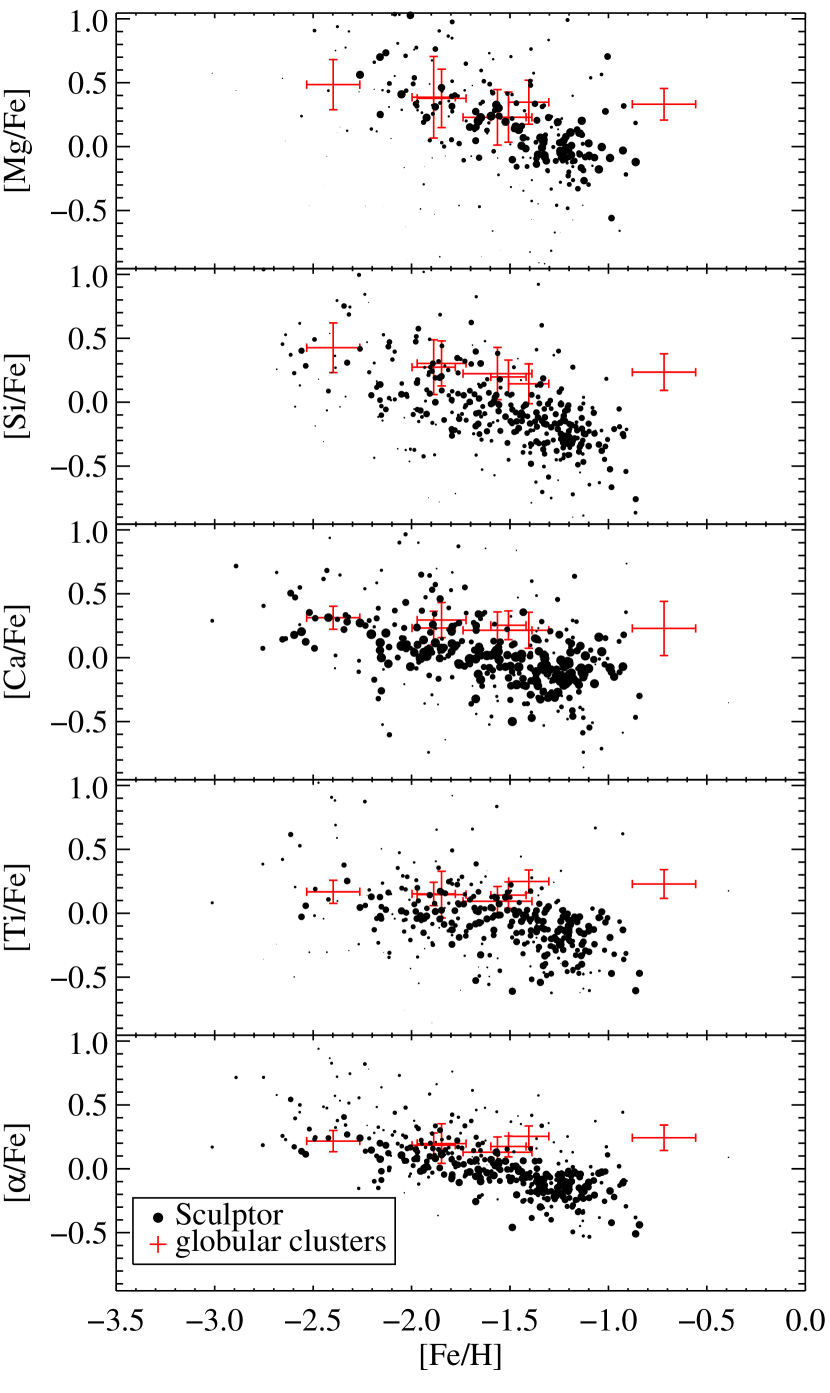
Figure 10.— Multi-element abundances in Sculptor (black). The point sizes reflect the quadrature sum of the errors on [Fe/H] and [X/Fe], where larger points have smaller errors. The bottom panel shows the average of the four elements shown in the other panels. For comparison, the red error bars show the means and standard deviations from the seven GCs of KGS08. Because the Sculptor and GC abundances were measured in the same way, the comparison demonstrates that [X/Fe] declines with increasing [Fe/H] in Sculptor, but not the GCs.

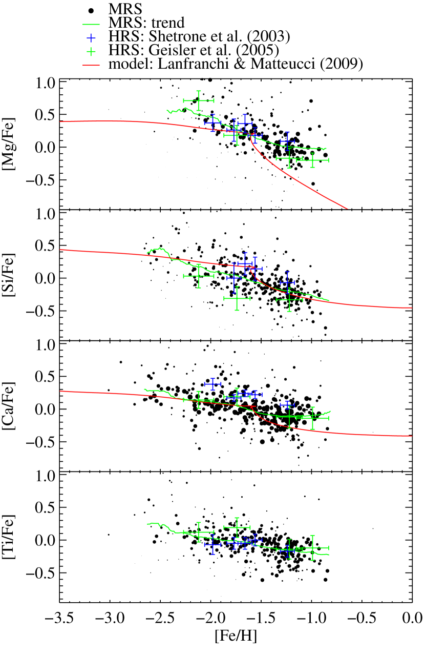
Figure 11.— As in Fig. 10, the black points show medium-resolution multi-element abundances in Sculptor. The points with error bars show published high-resolution data (Shetrone et al. 2003, blue, and Geisler et al. 2005, green). The green line is the inverse variance-weighted average of at least 20 stars within a window of $\Delta{\rm[Fe/H]}=0.25$. The red line shows the chemical evolution model of Lanfranchi & Matteucci (2004, updated 2009). The onset of Type Ia SNe causes the decline in [X/Fe] with [Fe/H]. Mg declines steadily because it is produced exclusively in Type II SNe, but Si, Ca, and Ti are produced in both Type Ia and II SNe.

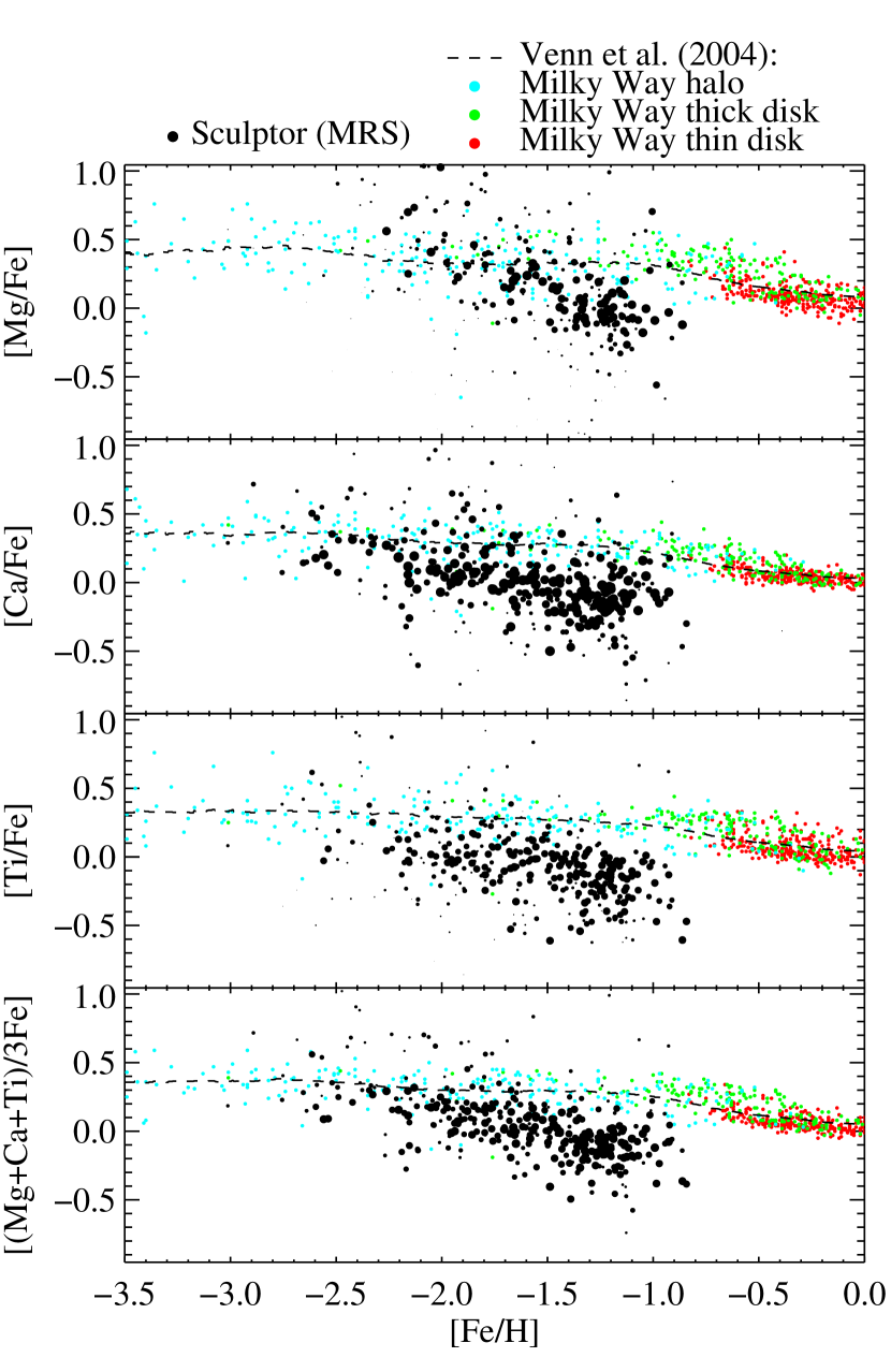
Figure 12.— As in Fig. 10, the black points show medium-resolution multi-element abundances in Sculptor. The colored points show different components of the Milky Way (Venn et al., 2004): the thin disk (red), the thick disk (green), and the field halo (cyan). The dashed lines are moving averages of the MW data in 0.75 dex bins of [Fe/H]. In Sculptor, [$\alpha$/Fe] falls at lower [Fe/H] than in the halo, indicating that the halo field stars were less polluted by Type Ia SNe and therefore formed more rapidly than Sculptor stars.

The discrepancy between halo and dSph abundances extends beyond the MDF. In the first HRS study of stars in a dSph, Shetrone, Bolte & Stetson (1998) found that the [Ca/Fe] ratio of metal-poor stars in Draco appeared solar, in contrast to the enhanced halo field stars. Shetrone, Côté & Sargent (2001) and Shetrone et al. (2003) confirmed the same result in Sextans (catalog NAME Sextans dSph), Ursa Minor, Sculptor, Fornax, Carina, and Leo I (catalog NAME LEO I dSph), and they included other $\alpha$ elements in addition to Ca.

Here, we present the largest sample of [$\alpha$/Fe] measurements in any dSph. Figure 10 shows [Mg/Fe], [Ca/Fe], and [Ti/Fe] versus [Fe/H] for Sculptor. The figure also shows the mean and standard deviations of all of the individual stellar abundance measurements for each of the seven GCs in the sample of KGS08. All of the modifications to the KGS08 technique described in Secs. 3 and 4 apply to the GC measurements in Fig. 10. Although our discussion in the appendix demonstrates that our measurements are accurate on an absolute scale by comparing to several different HRS studies in Sculptor, it is also instructive to compare abundances measured with the same technique in two types of stellar systems. All four element ratios slope downward with [Fe/H] in Sculptor but remain flat in the GCs. Additionally, the larger spread of [Mg/Fe] than other element ratios in the GCs is not due to larger measurement uncertainties but to the known intrinsic spread of Mg abundance in some GCs (see the review by Gratton et al., 2004). [Si/Fe], [Ca/Fe], and [Ti/Fe] are more slightly sloped than [Mg/Fe] in Sculptor because both Type Ia and Type II SNe produce Si, Ca, and Ti, but Type II SNe are almost solely responsible for producing Mg (Woosley & Weaver, 1995). Finally, to maximize the SNR of the element ratio measurements, we average the four ratios together into one number called [$\alpha$/Fe]. The [$\alpha$/Fe] ratio is flat across the GCs, but it decreases with increasing [Fe/H] in Sculptor.

Quantitative models of chemical evolution in dwarf galaxies are consistent with these trends. At a certain time corresponding to a certain [Fe/H] in the evolution of the dSph, Type Ia begin to pollute the interstellar medium with gas at subsolar [$\alpha$/Fe]. More metal-rich stars that form from this gas will have lower [$\alpha$/Fe] than the more metal-poor stars. Lanfranchi & Matteucci (2004) have developed a sophisticated model that includes SN feedback and winds. They predicted the abundance distributions of six dSphs, including Sculptor. Figure 11 shows our measurements with their predictions (updated with new SN yields, G. Lanfranchi 2009, private communication). As predicted, the range of [Mg/Fe] is larger than the range of [Ca/Fe] or [Si/Fe] because Mg is produced exclusively in Type II SNe whereas Si and Ca are produced in both Type Ia and II SNe (Woosley & Weaver, 1995). We do not observe strong evidence for a predicted sharp steepening in slope of both elements at ${\rm[Fe/H]}\sim-1.8$, but observational errors and intrinsic scatter may obscure this “knee.” Also, the observed [Fe/H] at which [Mg/Fe] begins to drop is higher than the model predicts, indicating a less intense wind than used in the model. Note that the element ratios [X/Fe] become negative (subsolar) at high enough [Fe/H], as predicted by the models. Lanfranchi & Matteucci (2004) do not predict [Ti/Fe] because it behaves more like an Fe-peak element than an $\alpha$ element.

In addition to trends of [$\alpha$/Fe] with [Fe/H], Marcolini et al. (2006, 2008) predicted the distribution functions of [Fe/H] and [$\alpha$/Fe] of a Draco-like dSph. The range of [Fe/H] they predicted is nearly identical to the range we observe in Sculptor, and the shapes of both distributions are similar. The outcome of the models depends on the mass of the dSph. Sculptor is ten times more luminous than Draco (Mateo, 1998) and therefore may have a larger total mass. [However, Strigari et al. (2008) find that all dSphs have the same dynamical mass within 300 pc of their centers. It is unclear whether the total masses of the original, unstripped dark matter halos are the same.] In principle, these chemical evolution models could be used to measure the time elapsed since different epochs of star formation and their durations. We defer such an analysis until the advent of a model based on a Sculptor-like luminosity or mass.

In Fig. 12, we compare individual stellar abundances in Sculptor to MW halo and disk field stars (compilation by Venn et al., 2004). As has been seen in many previous studies of individual stellar abundances in dSphs, [$\alpha$/Fe] falls at a significantly lower [Fe/H] in Sculptor than in the MW halo. The drop is particularly apparent in [Mg/Fe], which is the element ratio most sensitive to the ratio of the contributions of Type II to Type Ia SNe. The other element ratios also drop sooner in Sculptor than in the halo, but appear lower than in the halo at all metallicities. Along with the MDF comparison in Sec. 5.1.3, this result is consistent with the suggestion by Robertson et al. (2005) that galaxies significantly more massive than Sculptor built the inner MW halo. Their greater masses allowed them to retain more gas and experience more vigorous star formation. By the time Type Ia SNe diluted [$\alpha$/Fe] in the massive halo progenitors, the metallicity of the star-forming gas was already as high as ${\rm[Fe/H]}=-0.5$. In Sculptor, the interstellar [Fe/H] reached only $-1.5$ before the onset of Type Ia SNe pollution.

5.3. Radial Abundance Distributions

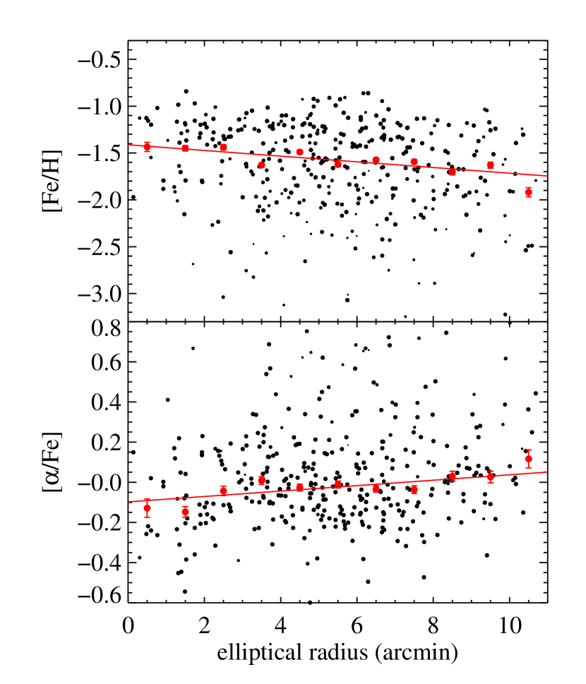
Figure 13.— Spatial abundance distributions in Sculptor. Point sizes are larger for stars with smaller measurement uncertainties. The red points reflect the mean values in 1 arcmin bins, along with the errors on the means. The red lines are the least-squares linear fits. We detect a gradient of $-0.030\pm 0.003$ dex per arcmin in [Fe/H] and $+0.013\pm 0.003$ dex per arcmin in [$\alpha$/Fe].

Because dSphs interact with the MW, they can lose gas through tidal or ram pressure stripping (Lin & Faber, 1983). The gas preferentially leaves from the dSph’s outskirts, where the gravitational potential is shallow. If the dSph experiences subsequent star formation, it must occur in the inner regions where gas remains. Sculptor’s MDF suggests a history of extended star formation. Sculptor might then be expected to exhibit a radial abundance gradient in the sense that the inner parts of the dSph are more metal-rich than the outer parts.

The detection of a radial metallicity gradient in Sculptor has been elusive. In a photometric study, Hurley-Keller (2000) found no evidence for an age or metallicity gradient. Based on HRS observations of five stars (the same sample as Shetrone et al., 2003), Tolstoy et al. (2003) found no correlation between [Fe/H] and spatial position. Finally, in a sample of 308 stars with CaT-based metallicities, T04 detected a significant segregation in Sculptor: a centrally concentrated, relatively metal-rich component and an extended, relatively metal-poor component. Westfall et al. (2006) arrived at the same conclusion, and Walker et al. (2009) confirmed the existence of a [Fe/H] gradient in a sample of 1365 Sculptor members.

In order to detect a gradient, those studies targeted Sculptor stars at distances of more than 20 arcmin. The maximum elliptical radius of this study is 11 arcmin. Therefore, this study is not ideally designed to detect radial gradients. Figure 13 shows the radial distribution of [Fe/H] and [$\alpha$/Fe] in Sculptor. The $x$-axis is the length of the semi-major axis of an ellipse defined by Sculptor’s position angle and ellipticity (Mateo, 1998). Although this study is limited in the spatial extent of targets, we do detect a gradient of $-0.030\pm 0.003$ dex per arcmin. This estimate is very close to the gradient observed by T04. Walker et al. (2009) measure a shallower gradient, but they present their results against circular radius instead of elliptical radius.

Marcolini et al. (2008) predict radial gradients in both [Fe/H] and [$\alpha$/Fe] in dSphs. In particular, they expect shallower [Fe/H] gradients for longer durations of star formation. The gradient we observe is stronger than any of their models. They also expect very few stars with low [$\alpha$/Fe] at large radius. Given that [$\alpha$/Fe] decreases with [Fe/H] and [Fe/H] decreases with distance, it seems reasonable to expect that [$\alpha$/Fe] increases with radius. In fact, we detect an [$\alpha$/Fe] gradient of $+0.013\pm 0.003$ dex per arcmin.

6. Conclusions

Sculptor is one of the best-studied dwarf spheroidal satellites of the Milky Way. In the past ten years, at least five spectroscopic campaigns at both low and high resolution have targeted this galaxy. More than any other dSph, Sculptor has aided in the understanding of the chemical evolution of dSphs and the construction of the Milky Way stellar halo.

We have sought to increase the sample of multi-element abundances in Sculptor through MRS. The advantages over HRS include higher throughput per resolution element, the ability to target fainter stars, and multiplexing. The large sample sizes will enable detailed comparisons to chemical evolution models of [$\alpha$/Fe] and [Fe/H] in dSphs. The disadvantages include larger uncertainties, particularly for elements with few absorption lines in the red, and the inability to measure many elements accessible to HRS. MRS is not likely to soon provide insight into the evolution of neutron-capture elements in dSphs.

In order to make the most accurate measurements possible, we have made a number of improvements to the technique of Kirby, Guhathakurta, & Sneden (2008a). We have consulted independent HRS of the same stars to confirm the accuracy of our measurements of [Fe/H], [Mg/Fe], [Ca/Fe], and [Ti/Fe]. In the case of [Fe/H] and the average [$\alpha$/Fe] our MRS measurements are only slightly more uncertain than HRS measurements.

Some of the products of this study include

1. An unbiased metallicity distribution for Sculptor. Because the synthesis-based abundances do not rely on any empirical calibration, their applicability is unrestricted with regard to [Fe/H] range. The MDF is asymmetric with a long, metal-poor tail, as predicted by chemical evolution models of dSphs. Furthermore, fits to simple chemical evolution models shows that Sculptor’s MDF is consistent with a model that requires no pre-enrichment.

2. The largest sample of [$\alpha$/Fe] and [Fe/H] measurements in any single dSph: 388 stars. We have confirmed the trend for [$\alpha$/Fe] to decrease with [Fe/H], as shown by Geisler et al. (2007) with just nine stars from the studies of Shetrone et al. (2003) and Geisler et al. (2005). Chemical evolution models may be constructed from these measurements to quantify the star formation history of Sculptor.

3. The detection of radial [Fe/H] and [$\alpha$/Fe] gradients. Our sample probes a smaller range than previous studies; nonetheless, we find a $-0.030\pm 0.003$ dex per arcmin gradient in [Fe/H] and a $+0.013\pm 0.003$ dex per arcmin gradient in [$\alpha$/Fe].

4. The discovery of a Sculptor member star with $\rm{\bf{[Fe/H]}}\mathbf{=-3.80\pm 0.28}$. This discovery suggests that since-disrupted galaxies similar to Sculptor may have played a role in the formation of the Milky Way metal-poor halo. High-resolution spectroscopy of individual stars will confirm or refute this indication.

Much more can be done with this technique in other galaxies. The stellar population of a dSph depends heavily on its stellar mass. For instance, Lanfranchi & Matteucci (2004) and Robertson et al. (2005) predict that more massive satellites have an [$\alpha$/Fe] “knee” at higher [Fe/H]. In the next papers in this series, we intend to explore the multi-element abundance distributions of other dSphs and compare them to each other. We will observe how the shapes of the MDFs and the [$\alpha$/Fe]–[Fe/H] diagrams change with dSph luminosity or stellar mass. These observations should aid our understanding of star formation, chemical evolution, and the construction of the Galaxy.

Appendix A Accuracy of the Abundance Measurements

In order to quantify the accuracy of the MRS measurements, we examine the spectra of stars observed more than once and stars with previous HRS measurements.

A.1. Duplicate Observations

Figure 14.— Cumulative distribution of differences between the repeat measurements of [Fe/H] for 17 stars divided by the estimated error of the difference. The curve is the integral of a unit Gaussian. The curve matches the distribution well, indicating that the errors are estimated properly.

Figure 15.— Same as Fig. 15 for [$\alpha$/Fe], which is the average of [Mg/Fe], [Si/Fe], [Ca/Fe], and [Ti/Fe].

The repeat observations of 17 stars provide insight on the effect of random error on the measurements of [Fe/H] and [$\alpha$/Fe]. Figures 15 and 15 summarize the comparisons of measurements of different spectra of the same stars. They show the cumulative distribution of the absolute difference between the measured [Fe/H] and [$\alpha$/Fe] for each pair of spectra divided by the expected error of the difference (see Sec. 4.9). The solid curve is the integral of a unit Gaussian, which represents the expected cumulative distribution if the estimated errors accurately represent the true measurement errors. In calculating the expected error of the difference, we apply the systematic error to only one of the two stars. Even though the same technique is used to measure abundances in both stars, some systematic error is appropriate because the wavelength range within a pair of spectra differs by 300–400 Å. The different Fe lines in these ranges span a different range of excitation potentials, and the Levenberg-Marquardt algorithm converges on different solutions.

A.2. Comparison to High-Resolution Measurements

Table 6Abundances of Stars with Previous High-Resolution Spectroscopy

star	$T_{\rm{eff}}$	$\log g$	$\xi$	[Fe/H]	[Mg/Fe]	[Si/Fe]	[Ca/Fe]	[Ti/Fe]
	(K)	(cm s-2)	(km s-1)	(dex)	(dex)	(dex)	(dex)	(dex)
Previous High-Resolution Measurements
H482	4400	1.10	1.70	$-1.24\pm 0.07$	$+0.09\pm 0.14$	$-0.07\pm 0.17$	$+0.06\pm 0.06$	$-0.17\pm 0.09$
H459	4500	1.00	1.65	$-1.66\pm 0.07$	$+0.36\pm 0.14$	$+0.22\pm 0.17$	$+0.24\pm 0.05$	$-0.05\pm 0.09$
H479	4325	0.70	1.70	$-1.77\pm 0.07$	$+0.26\pm 0.17$	$+0.00\pm 0.23$	$+0.17\pm 0.05$	$-0.05\pm 0.09$
H400	4650	0.90	1.70	$-1.98\pm 0.08$	$+0.37\pm 0.13$	$\cdots$	$+0.38\pm 0.09$	$-0.07\pm 0.15$
H461	4500	1.20	1.70	$-1.56\pm 0.07$	$+0.18\pm 0.12$	$+0.14\pm 0.18$	$+0.22\pm 0.06$	$+0.00\pm 0.09$
1446	3900	0.00	2.30	$-1.22\pm 0.13$	$-0.17\pm 0.15$	$-0.33\pm 0.18$	$-0.12\pm 0.17$	$-0.14\pm 0.15$
195	4250	0.20	1.80	$-2.12\pm 0.15$	$+0.71\pm 0.15$	$+0.03\pm 0.18$	$+0.14\pm 0.13$	$+0.12\pm 0.15$
982	4025	0.50	2.20	$-0.99\pm 0.16$	$-0.20\pm 0.11$	$\cdots$	$-0.14\pm 0.17$	$-0.12\pm 0.19$
770	4075	0.00	1.90	$-1.74\pm 0.13$	$+0.18\pm 0.15$	$-0.31\pm 0.18$	$+0.19\pm 0.13$	$+0.19\pm 0.15$
Medium-Resolution Measurements
H482	4347	0.83	1.95	$-1.24\pm 0.14$	$-0.03\pm 0.17$	$-0.16\pm 0.20$	$-0.19\pm 0.13$	$-0.12\pm 0.11$
H459	4390	1.12	1.88	$-1.88\pm 0.14$	$\cdots$	$-0.41\pm 0.48$	$+0.34\pm 0.27$	$+0.08\pm 0.18$
H479	4271	0.63	1.99	$-1.79\pm 0.14$	$+0.27\pm 0.42$	$-0.22\pm 0.22$	$+0.24\pm 0.18$	$-0.13\pm 0.11$
H400	4692	1.36	1.82	$-1.97\pm 0.15$	$\cdots$	$+0.58\pm 0.23$	$+0.90\pm 0.65$	$+0.10\pm 0.19$
H461	4313	0.78	1.96	$-1.81\pm 0.15$	$+0.36\pm 0.61$	$+0.05\pm 0.32$	$+0.39\pm 0.32$	$+0.25\pm 0.16$
1446	3838	0.49	2.03	$-1.22\pm 0.14$	$-0.03\pm 0.20$	$-0.07\pm 0.21$	$-0.05\pm 0.24$	$-0.40\pm 0.11$
195	4308	0.65	1.99	$-2.05\pm 0.14$	$+0.41\pm 0.17$	$+0.06\pm 0.19$	$+0.09\pm 0.10$	$+0.02\pm 0.11$
982	4147	0.52	2.02	$-0.84\pm 0.14$	$\cdots$	$\cdots$	$-0.30\pm 0.23$	$-0.47\pm 0.11$
770	4247	0.59	2.00	$-1.62\pm 0.14$	$+0.13\pm 0.29$	$-0.23\pm 0.21$	$+0.02\pm 0.11$	$-0.04\pm 0.11$

The most reliable test of the MRS atmospheric parameter and abundance estimates is to compare with completely independent observations and analyses of the same stars. Table 6 lists the previous HRS measurements of nine Sculptor members (Shetrone et al., 2003; Geisler et al., 2005) as well as the DEIMOS measurements of the same stars. Unfortunately, these two HRS studies share no stars in common and therefore cannot be compared with each other.

Figure 16.— Comparison between effective temperature ($T_{\rm{eff}}$) used in previous HRS abundance analyses and photometric $T_{\rm{eff}}$ used for this work’s MRS abundance analysis. Symbol shape indicates the reference for the HRS abundances. Star names from Tab. 1 are printed to the upper left of each point.

Figure 17.— Same as Fig. 17 except for surface gravity ($\log g$). The error bars represent photometric error, and they are given by replacing $T_{\rm{eff}}$ with $\log g$ in Eq. 6.

Figure 18.— Same as Fig. 17 except for microturbulent velocity ($\xi$). The error bars are found by propagating the error on $\log g$ through Eq. 2.

Figure 19.— Comparison between [Fe/H] derived from previous HRS abundance analyses and [Fe/H] derived from this work’s MRS abundance analysis. Symbols are the same as in Fig. 17.

Of $T_{\rm{eff}}$, $\log g$, and $\xi$, any spectroscopic abundance measurement is most sensitive to $T_{\rm{eff}}$. In general, underestimating $T_{\rm{eff}}$ leads to an underestimate of [Fe/H]. Shetrone et al. (2003, hereafter S03) determine $T_{\rm{eff}}$ spectroscopically by minimizing the slope of the derived abundance for each line versus excitation potential. Geisler et al. (2005, hereafter G05) determine $T_{\rm{eff}}$ photometrically with empirical color-temperature relations. Figure 17 shows $T_{\rm{eff}}$ from those studies and this one for each of the nine stars in common. The MRS temperatures do not follow the temperatures of either HRS study better than the other.

Both S03 and G05 measure $\log g$ spectroscopically from demanding ionization equilibrium: [Fe/H] measured from Fe I lines must match that measured from Fe II lines. However, our red spectra have very few measurable Fe II lines. Alternatively, $\log g$ may be determined from a star’s absolute magnitude and $T_{\rm{eff}}$ via the Stefan-Boltzmann law. Even though gravity depends on the inverse square of $T_{\rm{eff}}$ and the inverse square root of luminosity, luminosity imposes a stronger constraint on $\log g$ because of its larger range on the RGB than $T_{\rm{eff}}$. Even accounting for the error in the distance modulus to Sculptor, the typical error on photometric $\log g$ is $\sim 0.1$ dex. Therefore, we determine $\log g$ from photometry alone. Figure 17 shows the comparison between $\log g$ used by S03 and G05 and this study. The agreement is not particularly good, with discrepancies up to 0.6 dex. However, the photometric values of $\log g$ are more accurate than can be determined from the medium-resolution red spectra, which show very few lines of ionized species. Furthermore, as discussed below, errors in $\log g$ influence the abundance measurements much less than errors in $T_{\rm{eff}}$.

Both S03 and G05 measure microturbulent velocity ($\xi$) by forcing all Fe lines to give the same abundance regardless of their reduced width. We have fixed $\xi$ to $\log g$ with an empirical relation (Eq. 2). Figure 19 compares the HRS microturbulent velocities ($\xi$) to our adopted values. The largest discrepancy is 0.3 km s^-1.

Figure 19 shows the comparison between HRS and MRS [Fe/H] measurements for the same stars. The agreement is very good ($\sigma=0.14$ dex). Just two stars out of nine do not fall within $1\sigma$ of the one-to-one line.

The MRS [Fe/H] for star 770 is larger than the HRS [Fe/H]. The MRS $T_{\rm{eff}}$ is also significantly larger than the HRS $T_{\rm{eff}}$ for this star. Similarly, the MRS $T_{\rm{eff}}$ for star H461 is lower than the HRS $T_{\rm{eff}}$, forcing the MRS [Fe/H] lower than the HRS [Fe/H]. In fact, even the smaller deviations from the [Fe/H] one-to-one line can be attributed to deviations from the $T_{\rm{eff}}$ one-to-one line. No such correlation can be attributed to deviations in $\log g$ or $\xi$. The close correspondence between Figs. 17 and 19 demonstrates that $T_{\rm{eff}}$ is the dominant atmospheric parameter in determining metallicity.

Figure 20.— Comparison between the HRS spectral synthesis measurements of [Fe/H] of Battaglia et al. (2008b) and the synthesis-based medium resolution measurements of [Fe/H] (this work) for the stars observed in both studies.

B08b published a catalog of VLT/FLAMES [Fe/H] measurements based on both the EW of the infrared Ca II triplet (CaT) and HRS (Hill et al., in preparation). The two resolution modes of FLAMES ($R\sim 6500$ and $R\sim 20000$) allowed them to complete both MRS and HRS analyses with the same instrument. Their high-resolution spectroscopic sample and ours overlap by 47 stars, which are shown in Fig. 20. The agreement ($\sigma=0.14$ dex) is as good as the previous comparison to HRS studies.

The B08b HRS measurements rely on atmospheric parameters determined from both five-band photometry and spectroscopy. We also measure $T_{\rm{eff}}$ spectrophotometrically. Our methods may be similar, although we do not use infrared photometry. There appears to be a small systematic trend such that our MRS measurements are lower than the B08b HRS measurements of [Fe/H] at both low and high [Fe/H]. The average discrepancy at the extrema of the residuals is 0.2 dex. We withhold a detailed investigation of these residuals until publication of the details of the HRS study.

B08b share seven stars in common with S03 and G05. To emphasize the accuracy of our MRS analysis, we note that the scatter of the differences between the two sets of HRS studies ($\sigma=0.16$ dex) is in fact larger than the scatter in the comparison between the MRS [Fe/H] and the same seven stars of S03 and G05 ($\sigma=0.14$ dex). This small sample does not indicate that the MRS measurements are more accurate than any HRS measurements, but it does suggest that the accuracy is competitive.

Figure 21.— Same as Fig. 19 except for [Mg/Fe] (upper left), [Si/Fe] (upper right), [Ca/Fe] (lower left), and [Ti/Fe] (lower right). Only those measurements with estimated errors less than 0.45 dex are shown.

Figure 22.— Same as Fig. 19 except for an average of the $\alpha$ elements.

Figure 23.— Comparison between the HRS measurements of [Ca/Fe] of Battaglia et al. (2008b) and the synthesis-based medium resolution measurements of [Ca/Fe] (this work) for the stars observed in both studies.

Figure 21 shows the comparison between the MRS and HRS (S03 and G05) values of [Mg/Fe], [Si/Fe], [Ca/Fe], and [Ti/Fe]. In addition, Fig. 23 shows unweighted averages of those four element ratios where available. The agreement is good in all cases. Furthermore, the error bars seem to be reasonable estimates of the actual random and systematic error.

The agreement between HRS and MRS [$\alpha$/Fe] is very good ($\sigma=0.13$ dex). Even though Fe lines outnumber $\alpha$ elements lines, the ratio [$\alpha$/Fe] can be measured about as accurately as [Fe/H] because $\alpha$ and Fe respond similarly to errors in atmospheric parameters whereas $T_{\rm{eff}}$ and [Fe/H] exhibit strong covariance.

In addition to [Fe/H], B08b have published HRS measurements of [Ca/Fe]. Figure 23 shows the comparison between the stars we share in common ($\sigma=0.20$ dex). The larger vertical scatter than horizontal scatter demonstrates that an MRS analysis is noisier than an HRS analysis when the number of measurable lines is small. Regardless, the degree of correlation is high, with a linear Pearson correlation coefficient of 0.53, indicating that the medium-resolution spectra have significant power to constrain [Ca/Fe].

Table 6Multi-Element Abundances in Sculptor

RA	Dec	$M$	$T_{2}$	$T_{\rm{eff}}$	$\log g$	$\xi$	[Fe/H]	[Mg/Fe]	[Si/Fe]	[Ca/Fe]	[Ti/Fe]
				(K)	(cm s-2)	(km s-1)	(dex)	(dex)	(dex)	(dex)	(dex)
$00^{\mathrm{h}}59^{\mathrm{m}}21\fs 6$	$-33\arcdeg 42\arcmin 58\arcsec$	$19.662\pm 0.090$	$18.557\pm 0.048$	5105	2.02	1.66	$-2.17\pm 0.19$	$\cdots$	$-0.12\pm 0.75$	$+0.39\pm 0.28$	$\cdots$
$00^{\mathrm{h}}59^{\mathrm{m}}21\fs 7$	$-33\arcdeg 41\arcmin 02\arcsec$	$18.296\pm 0.037$	$16.987\pm 0.027$	4674	1.27	1.84	$-1.91\pm 0.14$	$+0.05\pm 0.41$	$+0.07\pm 0.21$	$+0.06\pm 0.15$	$+0.14\pm 0.14$
$00^{\mathrm{h}}59^{\mathrm{m}}23\fs 9$	$-33\arcdeg 42\arcmin 59\arcsec$	$19.614\pm 0.091$	$18.383\pm 0.048$	4805	1.87	1.70	$-1.95\pm 0.16$	$+0.27\pm 0.64$	$-0.12\pm 0.39$	$+0.37\pm 0.22$	$-0.04\pm 0.37$
$00^{\mathrm{h}}59^{\mathrm{m}}26\fs 9$	$-33\arcdeg 40\arcmin 29\arcsec$	$18.871\pm 0.051$	$17.559\pm 0.029$	4672	1.49	1.79	$-1.21\pm 0.14$	$-0.48\pm 0.47$	$-0.06\pm 0.20$	$-0.03\pm 0.14$	$-0.00\pm 0.13$
$00^{\mathrm{h}}59^{\mathrm{m}}27\fs 1$	$-33\arcdeg 43\arcmin 42\arcsec$	$17.872\pm 0.026$	$16.327\pm 0.024$	4392	0.88	1.93	$-1.67\pm 0.14$	$+0.05\pm 0.22$	$-0.19\pm 0.20$	$-0.01\pm 0.13$	$-0.08\pm 0.11$
$00^{\mathrm{h}}59^{\mathrm{m}}27\fs 3$	$-33\arcdeg 38\arcmin 47\arcsec$	$18.218\pm 0.037$	$16.927\pm 0.028$	4738	1.26	1.84	$-1.51\pm 0.14$	$+0.41\pm 0.38$	$-0.32\pm 0.23$	$+0.02\pm 0.15$	$+0.02\pm 0.13$
$00^{\mathrm{h}}59^{\mathrm{m}}27\fs 7$	$-33\arcdeg 40\arcmin 35\arcsec$	$17.383\pm 0.025$	$15.699\pm 0.025$	4232	0.60	2.00	$-2.16\pm 0.14$	$+0.25\pm 0.21$	$+0.14\pm 0.19$	$+0.12\pm 0.12$	$-0.03\pm 0.11$
$00^{\mathrm{h}}59^{\mathrm{m}}28\fs 3$	$-33\arcdeg 42\arcmin 07\arcsec$	$17.305\pm 0.017$	$15.377\pm 0.020$	3789	0.49	2.03	$-1.65\pm 0.14$	$+0.23\pm 0.15$	$+0.30\pm 0.19$	$-0.17\pm 0.13$	$-0.33\pm 0.10$
$00^{\mathrm{h}}59^{\mathrm{m}}28\fs 7$	$-33\arcdeg 38\arcmin 57\arcsec$	$19.063\pm 0.037$	$17.763\pm 0.030$	4622	1.58	1.77	$-1.76\pm 0.14$	$\cdots$	$+0.07\pm 0.24$	$-0.04\pm 0.16$	$+0.08\pm 0.15$
$00^{\mathrm{h}}59^{\mathrm{m}}30\fs 4$	$-33\arcdeg 36\arcmin 05\arcsec$	$18.108\pm 0.024$	$16.705\pm 0.021$	4517	1.11	1.88	$-2.49\pm 0.15$	$\cdots$	$-0.19\pm 1.22$	$+0.31\pm 0.21$	$+0.19\pm 0.22$

Note. — Table 6 is published in its entirety in the electronic edition of the Astrophysical Journal. A portion is shown here for guidance regarding form and content.

References

- Anders & Grevesse (1989) Anders, E., & Grevesse, N. 1989, Geochim. Cosmochim. Acta, 53, 197
- Battaglia et al. (2008a) Battaglia, G., Helmi, A., Tolstoy, E., Irwin, M., Hill, V., & Jablonka, P. 2008a, ApJ, 681, L13
- Battaglia et al. (2008b) Battaglia, G., Irwin, M., Tolstoy, E., Hill, V., Helmi, A., Letarte, B., & Jablonka, P. 2008b, MNRAS, 383, 183 (B08b)
- Battaglia et al. (2006) Battaglia, G., et al. 2006, A&A, 459, 423
- Castelli (2005) Castelli, F. 2005, Memorie della Societa Astronomica Italiana Supplement, 8, 34
- Castelli et al. (1997) Castelli, F., Gratton, R. G., & Kurucz, R. L. 1997, A&A, 318, 841
- Castelli & Kurucz (2004) Castelli, F., & Kurucz, R. L. 2004, ArXiv Astrophysics e-prints, arXiv:astro-ph/0405087
- Cohen & Huang (2009) Cohen, J. G., & Huang, W. 2009, ApJ, 701, 1053
- Demarque et al. (2004) Demarque, P., Woo, J.-H., Kim, Y.-C., & Yi, S. K. 2004, ApJS, 155, 667
- Faber et al. (2003) Faber, S. M., et al. 2003, Proc. SPIE, 4841, 1657
- Font et al. (2006) Font, A. S., Johnston, K. V., Bullock, J. S., & Robertson, B. E. 2006, ApJ, 638, 585
- Frebel et al. (2008) Frebel, A., Collet, R., Eriksson, K., Christlieb, N., & Aoki, W. 2008, ApJ, 684, 588
- Frebel et al. (2009) Frebel, A. F., et al. 2009, ApJ, submitted, arXiV:0902.2395
- Fuhr & Wiese (2006) Fuhr, J. R., & Wiese, W. L. 2006, Journal of Physical and Chemical Reference Data, 35, 1669
- Fulbright (2000) Fulbright, J. P. 2000, AJ, 120, 1841
- Geisler et al. (2005) Geisler, D., Smith, V. V., Wallerstein, G., Gonzalez, G., & Charbonnel, C. 2005, AJ, 129, 1428 (G05)
- Geisler et al. (2007) Geisler, D., Wallerstein, G., Smith, V. V., & Casetti-Dinescu, D. I. 2007, PASP, 119, 939
- Girardi et al. (2002) Girardi, L., Bertelli, G., Bressan, A., Chiosi, C., Groenewegen, M. A. T., Marigo, P., Salasnich, B., & Weiss, A. 2002, A&A, 391, 195
- Gratton et al. (2004) Gratton, R., Sneden, C., & Carretta, E. 2004, ARA&A, 42, 385
- Grevesse & Sauval (1998) Grevesse, N., & Sauval, A. J. 1998, Space Science Reviews, 85, 161
- Guhathakurta et al. (2006) Guhathakurta, P., et al. 2006, AJ, 131, 2497
- Helmi et al. (2006) Helmi, A., et al. 2006, ApJ, 651, L121 (H06)
- Holtzman et al. (2006) Holtzman, J. A., Afonso, C., & Dolphin, A. 2006, ApJS, 166, 534
- Hurley-Keller (2000) Hurley-Keller, D. A. 2000, Ph.D. Thesis, University of Michigan
- Johnson (2002) Johnson, J. A. 2002, ApJS, 139, 219
- Kirby (2009) Kirby, E. N. 2009, Ph.D. Thesis, University of California Santa Cruz
- Kirby et al. (2008a) Kirby, E. N., Guhathakurta, P., & Sneden, C. 2008a, ApJ, 682, 1217 (KGS08)
- Kirby et al. (2008b) Kirby, E. N., Simon, J. D., Geha, M., Guhathakurta, P., & Frebel, A. 2008b, ApJ, 685, L43
- Koch et al. (2008) Koch, A., Grebel, E. K., Gilmore, G. F., Wyse, R. F. G., Kleyna, J. T., Harbeck, D. R., Wilkinson, M. I., & Wyn Evans, N. 2008, AJ, 135, 1580
- Kurucz (1993) Kurucz, R. 1993, ATLAS9 Stellar Atmosphere Programs and 2 km/s grid. Kurucz CD-ROM No. 13. Cambridge, Mass.: Smithsonian Astrophysical Observatory, 1993, 13
- Lai et al. (2007) Lai, D. K., Johnson, J. A., Bolte, M., & Lucatello, S. 2007, ApJ, 667, 1185
- Lanfranchi & Matteucci (2004) Lanfranchi, G. A., & Matteucci, F. 2004, MNRAS, 351, 1338
- Lin & Faber (1983) Lin, D. N. C., & Faber, S. M. 1983, ApJ, 266, L21
- Lynden-Bell (1975) Lynden-Bell, D. 1975, Vistas in Astronomy, 19, 299
- Majewski et al. (2000) Majewski, S. R., Ostheimer, J. C., Kunkel, W. E., & Patterson, R. J. 2000, AJ, 120, 2550
- Marcolini et al. (2008) Marcolini, A., D’Ercole, A., Battaglia, G., & Gibson, B. K. 2008, MNRAS, 386, 2173
- Marcolini et al. (2006) Marcolini, A., D’Ercole, A., Brighenti, F., & Recchi, S. 2006, MNRAS, 371, 643
- Markwardt (2009) Markwardt, C. B. 2009, in ASP Conf. Ser., arXiv:0902.2850, Astronomical Data Analysis Software and Systems XVIII, ed. D. Bohlender, P. Dowler, & D. Durand (San Francisco, CA: ASP)
- Mateo (1998) Mateo, M. L. 1998, ARA&A, 36, 435
- Norris et al. (2008) Norris, J. E., Gilmore, G., Wyse, R. F. G., Wilkinson, M. I., Belokurov, V., Evans, N. W., & Zucker, D. B. 2008, ApJ, 689, L113
- Pagel (1997) Pagel, B. E. J. 1997, Nucleosynthesis and Chemical Evolution of Galaxies (Cambridge UP)
- Pietrzyński et al. (2008) Pietrzyński, G., et al. 2008, AJ, 135, 1993
- Prantzos (2003) Prantzos, N. 2003, A&A, 404, 211
- Prantzos (2008) Prantzos, N. 2008, A&A, 489, 525
- Queloz et al. (1995) Queloz, D., Dubath, P., & Pasquini, L. 1995, A&A, 300, 31
- Ramírez & Meléndez (2005) Ramírez, I., & Meléndez, J. 2005, ApJ, 626, 465
- Robertson et al. (2005) Robertson, B., Bullock, J. S., Font, A. S., Johnston, K. V., & Hernquist, L. 2005, ApJ, 632, 872
- Salvadori & Ferrara (2009) Salvadori, S., & Ferrara, A. 2009, MNRAS, 395, L6
- Schlegel et al. (1998) Schlegel, D. J., Finkbeiner, D. P., & Davis, M. 1998, ApJ, 500, 525
- Schmidt (1963) Schmidt, M. 1963, ApJ, 137, 758
- Schoerck et al. (2008) Schoerck, T., et al. 2008, A&A, submitted, arXiv:0809.1172
- Searle & Zinn (1978) Searle, L., & Zinn, R. 1978, ApJ, 225, 357
- Shetrone et al. (1998) Shetrone, M. D., Bolte, M., & Stetson, P. B. 1998, AJ, 115, 1888
- Shetrone et al. (2001) Shetrone, M. D., Côté, P., & Sargent, W. L. W. 2001, ApJ, 548, 592
- Shetrone et al. (2009) Shetrone, M. D., Siegel, M. H., Cook, D. O., & Bosler, T. 2009, AJ, 137, 62
- Shetrone et al. (2003) Shetrone, M. D., Venn, K. A., Tolstoy, E., Primas, F., Hill, V., & Kaufer, A. 2003, AJ, 125, 684 (S03)
- Simon & Geha (2007) Simon, J. D., & Geha, M. 2007, ApJ, 670, 313
- Sneden (1973) Sneden, C. A. 1973, Ph.D. Thesis, University of Texas at Austin
- Sneden et al. (1992) Sneden, C., Kraft, R. P., Prosser, C. F., & Langer, G. E. 1992, AJ, 104, 2121
- Strigari et al. (2008) Strigari, L. E., Bullock, J. S., Kaplinghat, M., Simon, J. D., Geha, M., Willman, B., & Walker, M. G. 2008, Nature, 454, 1096
- Thévenin & Idiart (1999) Thévenin, F., & Idiart, T. P. 1999, ApJ, 521, 753
- Tolstoy et al. (2003) Tolstoy, E., et al. 2003, AJ, 125, 707
- Tolstoy et al. (2004) Tolstoy, E., et al. 2004, ApJ, 617, L119 (T04)
- van den Bergh (1962) van den Bergh, S. 1962, AJ, 67, 486
- VandenBerg et al. (2006) VandenBerg, D. A., Bergbusch, P. A., & Dowler, P. D. 2006, ApJS, 162, 375
- Venn & Hill (2005) Venn, K. A., & Hill, V. M. 2005, From Lithium to Uranium: Elemental Tracers of Early Cosmic Evolution, 228, 513
- Venn & Hill (2008) Venn, K. A., & Hill, V. M. 2008, The Messenger, 134, 23
- Venn et al. (2004) Venn, K. A., Irwin, M., Shetrone, M. D., Tout, C. A., Hill, V., & Tolstoy, E. 2004, AJ, 128, 1177
- Walker et al. (2009) Walker, M. G., Mateo, M., & Olszewski, E. W. 2009, AJ, 137, 3100
- Walker et al. (2007) Walker, M. G., Mateo, M., Olszewski, E. W., Gnedin, O. Y., Wang, X., Sen, B., & Woodroofe, M. 2007, ApJ, 667, L53
- Westfall et al. (2006) Westfall, K. B., Majewski, S. R., Ostheimer, J. C., Frinchaboy, P. M., Kunkel, W. E., Patterson, R. J., & Link, R. 2006, AJ, 131, 375
- White & Rees (1978) White, S. D. M., & Rees, M. J. 1978, MNRAS, 183, 341
- Woosley & Weaver (1995) Woosley, S. E., & Weaver, T. A. 1995, ApJS, 101, 181