An exact renormalization formula for Gaussian exponential sums and applications

Abstract.

In the present paper, we derive a renormalization formula “à la Hardy-Littlewood” for the Gaussian exponential sums with an exact formula for the remainder term. We use this formula to describe the typical growth of the Gaussian exponential sums.

Résumé. Dans cet article, nous obtenons une formule de renormalisation “à la Hardy-Littlewood” pour des sommes exponentielles gaussiennes avec une formule exacte pour les termes de reste. Nous utilisons cette formule pour décrire la croissance typique de ces sommes.

Let $(a,b)\in(0,1)\times(-1/2,1/2]$ and consider the Gaussian exponential sum

(0.1) $$S(N,a,b)=\sum_{0\leq n\leq N-1}e\left(-\frac{an^{2}}{2}+nb\right),\quad N=1,2,3\dots.$$

where $e(z)=e^{2\pi iz}$. We set $S(0,a,b)=0$.
Such sums have been the object of many studies (see e.g. [8, 6, 9, 12, 13]) and have applications in various fields of mathematics and physics. In the present paper we prove a renormalization formula (see Theorem 2.1) analogous to the one first introduced in [8]. In our formula the “remainder term” is given explicitly by a special function (see section 1). We use this renormalization formula to obtain results on the typical growth and on the graphs of the exponential sums (0.1) (see Figure 2).
Let us now present our main results on the growth of $S(N,a,b)$. To our knowledge, up to the present work, the growth was studied mainly in the case $b=0$ ([6, 12]). As we shall see, the nontrivial $b$ does change the rate of growth. We prove

Theorem 0.1.

Let $g:{\mathbb{R}}_{+}\to{\mathbb{R}}_{+}$ be a non increasing function. Then, for almost every $(a,b)\in(0,1)\times(-1/2,1/2]$,

(0.2) $$\limsup_{N\to+\infty}\left(g(\ln N)\,\frac{|S(N,a,b)\,|}{\sqrt{N}}\right)<\infty\quad\Longleftrightarrow\quad\sum_{l\geq 1}g^{6}(l)<\infty.$$

This result should be compared with the following theorem for the exponential sum $S(N,a,b)$ for $b$ in the set

$$B_{a}=\left\{\{\frac{1}{2}(ma+n)\}_{0};\ (m,n)\in{\mathbb{Z}}^{2}\setminus(2{\mathbb{Z}}+1)^{2}\right\}$$

where, for $x\in{\mathbb{R}}$, $\{x\}_{0}=x\,{\rm mod}\,1$ and $-1/2<\{x\}_{0}\leq 1/2$. For every irrational $a$, the set $B_{a}$ is dense in $(-1/2,1/2]$ as the set $\{ma+n;\ (m,n)\in{\mathbb{Z}}^{2}\}$ is dense in ${\mathbb{R}}$.
One has

Theorem 0.2.

Let $g:{\mathbb{R}}_{+}\to{\mathbb{R}}_{+}$ be a non increasing function. Then, for almost all $a\in(0,1)$, there exists a dense $G_{\delta}$, say $\tilde{B}_{a}$, such that $B_{a}\subset\tilde{B}_{a}$ and, for $b\in\tilde{B}_{a}$, one has

$$\limsup_{N\to+\infty}\left(g(\ln N)\,\frac{|S(N,a,b)\,|}{\sqrt{N}}\right)<\infty\quad\Longleftrightarrow\quad\sum_{l\geq 1}g^{4}(l)<\infty.$$

For $b=0\in B_{a}$, Theorem 0.2 was proved in [6].
Let $\varphi(N)=(\ln N)^{1/4}$. Theorems 0.1 and 0.2 show that for a typical $a$, whereas for $b\in\tilde{B}_{a}$ the ratio $S(N,a,b)/\sqrt{N}$ grows faster than $\varphi(N)$, for a typical $b$, the ratio $S(N,a,b)/\sqrt{N}$ grows slower than $(\,\varphi(N)\,)^{2/3+\varepsilon}$ for any $\varepsilon>0$.

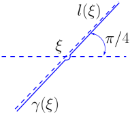
Figure 1. The path

The paper is organized as follows. In section 1, we describe the special function mentioned above. Then, section 2 is devoted to the exact renormalization formula, its proof and some useful consequences. It is then used in section 3 to compute asymptotics for $S(N,a,b)$ when an element of the continuous fraction defining $a$ is large. Section 3.3 is devoted to the discussion of the graphs of the quadratic sums and the appearance of the Cornu spiral. In section 4, we compute precise estimates of $S(N,a,b)$ in terms of the trajectory of a dynamical system related to the continued fractions expansion of $a$. Finally, sections 5 and 6 are devoted to the proofs of Theorems 0.1 and 0.2. The proofs are based on the estimates obtained in the previous section and on the analysis of certain dynamical systems.

1. The special function ${\mathcal{F}}$

Consider the function ${\mathcal{F}}:{\mathbb{C}}\to{\mathbb{C}}$ defined by

(1.1) $$\hskip-85.35826pt{\mathcal{F}}(\xi,a)=\int_{\gamma(\xi)}\frac{e\left(\frac{p^{2}}{2a}\right)\,dp}{e(p-\xi)-1}$$

where the contour $\gamma(\xi)$ is going up from infinity along $l(\xi)$, the strait line $\xi+e^{i\pi/4}{\mathbb{R}}$, coming infinitesimally close to the point $\xi$, then, going around this point in the anti-clockwise direction along an infinitesimally small semi-circle, and, then, going up to infinity again along $l(\xi)$ (see Fig. 1).
The function ${\mathcal{F}}$ is the special function mentioned in the introduction. We prove:

Lemma 1.1.

For each $a>0$,  ${\mathcal{F}}$ is an entire function of $\xi$, and, for all
$\xi\in{\mathbb{C}}$, one has

(1.2) $${\mathcal{F}}(\xi,a)-{\mathcal{F}}(\xi-1,a)=e\left(\frac{\xi^{2}}{2a}\right),$$

(1.3) $${\mathcal{G}}(\xi+a,a)-{\mathcal{G}}(\xi,a)=e\left(-\frac{\xi^{2}}{2a}\right),$$

where

(1.4) $${\mathcal{G}}(\xi,a)=c(a)\,e\left(-\frac{\xi^{2}}{2a}\right)\,{\mathcal{F}}(\xi,a),\quad c(a)=e(-1/8)\,a^{-1/2},$$

and

(1.5) $${\mathcal{F}}(-\xi,a)+{\mathcal{F}}(\xi,a)=e\left(\frac{\xi^{2}}{2a}\right)-\frac{1}{c(a)}.$$

Proof.

The first relation (1.2) follows from the residue theorem. The second relation (1.3) becomes obvious after the change of variable $z=p-\xi$ in the integral defining ${\mathcal{F}}$. To get the last relation, in the integral representing ${\mathcal{F}}(-\xi,a)$, we change the variable $p\to-p$, and then, using the residue theorem, we get

$${\mathcal{F}}(-\xi,a)=e\left(\frac{\xi^{2}}{2a}\right)-\int_{\gamma(\xi)}\frac{e\left(\frac{p^{2}}{2a}\right)\,e(p-\xi)\,dp}{e(p-\xi)-1}.$$

This and (1.1) implies (1.5). This completes the proof of Lemma 1.1. ∎

Lemma 1.1 shows that the function ${\mathcal{F}}$ simultaneously satisfies two difference equations, (1.2) and (1.3), with two different shift parameters, $1$ and $a$. This leads to the renormalization described in the next section.
For small $a$, the asymptotics of ${\mathcal{F}}$ are described by

Proposition 1.1.

Let $-1/2\leq\xi\leq 1/2$ and $0<a<1$. Then, ${\mathcal{F}}$ admits the representation:

(1.6) $$\begin{split}{\mathcal{F}}(\xi,a)&=e(1/8)\,f(a^{-1/2}\xi)+O(a^{1/2}),\\ f(t)&:=e(t^{2}/2)F(t)\text{ and }F(t):=\int_{-\infty}^{t}e(-\tau^{2}/2)\,d\tau,\end{split}$$

where $O(a^{1/2})$ is bounded by $C\,a^{1/2}$, and $C$ is a constant independent of $a$ and $\xi$.

This is Proposition 1.1 in [5]; for the readers convenience, we repeat its short proof below.
For small values of $a$, the special function ${\mathcal{F}}$ “becomes” the Fresnel integral. This proposition and our renormalization formula immediately explain the curlicues seen in the graphs of the exponential sums (see e.g. [14, 1]). Details can be found in section 3.3 and in [5].

Proof of Proposition 1.1.

We represent ${\mathcal{F}}$ in the form:

(1.7) $${\mathcal{F}}(\xi,a)=\frac{1}{2\pi i}\int_{\gamma(\xi)}\frac{e\left(\frac{p^{2}}{2a}\right)\,dp}{p-\xi}+\int_{\gamma(\xi)}g(p-\xi)\,e\left(\frac{p^{2}}{2a}\right)\,dp,$$

where

$$g(p-\xi)=\frac{1}{e(p-\xi)-1}-\frac{1}{2\pi i(p-\xi)}.$$

As $-1/2\leq\xi\leq 1/2$, the integration contour in the second integral can be deformed into the curve $\gamma(0)$ without intersecting any pole of the integrand. Then, the distance between the integration contour and these poles becomes bounded from below by $1/2^{3/2}$, and one easily gets $|g(p-\xi)|\leq C$ uniformly in $-1/2\leq\xi\leq 1/2$ and in $p\in\gamma(0)$. This immediately implies that the second term in (1.7) is bounded by $C\,a^{1/2}$. Finally, it is easily seen that first term satisfies the equation $I^{\prime}(\xi)=e(1/8)a^{-1/2}+2i\pi\xi a^{-1}I(\xi)$, and that it tends to $0$ when $\xi\to-\infty$ along ${\mathbb{R}}$. This implies that this term is equal to $e(1/8)\,f(a^{-1/2}\xi)$ and completes the proof of Proposition 1.1. ∎

2. Exact renormalization formulas

We now present exact renormalization formulas for the quadratic exponential sum $S(N,a,b)$ in terms of the special function ${\mathcal{F}}(\xi,a)$.

2.1. One renormalization

One has

Theorem 2.1.

Fix $N\in{\mathbb{N}}$ and $(a,b)\in(0,1)\times(-1/2,1/2]$. Let

$$\xi=\{aN\},\quad N_{1}=[aN],$$

(2.1) $$a_{1}=\left\{\frac{1}{a}\right\},\quad\quad b_{1}\equiv\left\{-\frac{b}{a}+\frac{1}{2}\,\left[\frac{1}{a}\right]\right\}_{0},$$

where $\{x\}$ and $\left[x\right]$ denote the fractional and the integer parts of the real number $x$, and $\{x\}_{0}=x\,{\rm mod}\,1$ and $-1/2<\{x\}_{0}\leq 1/2$. Then,

(2.2) $$\begin{split}S(N,a,b)&=c(a)\left[e\left(\frac{b^{2}}{2a}\right)\overline{S(N_{1},a_{1},b_{1})}\right.\\ &\hskip 28.45274pt\left.+e\left(-\frac{aN^{2}}{2}+Nb\right)\,{\mathcal{F}}(\xi-b,a)-{\mathcal{F}}(-b,a)\right].\end{split}$$

To our knowledge, such renormalization formulas (though without explicit description of the terms containing $\mathcal{F}$) first appeared in [8] and have since then a long tradition. The formula (2.2) is analogous to the less general one derived in [5]. It should also be compared to Theorems 4 and 5 in [6].

Proof of Theorem 2.1.

The idea of the proof is to compute the quantity ${\mathcal{F}}(Na-b,a)$ in two different ways: first, using (1.3), and then, using (1.2).
By means of (1.3), we get

$${\mathcal{G}}(Na-b,b) =\sum_{k=0}^{N-1}e\,\left(-\frac{(ka-b)^{2}}{2a}\right)+{\mathcal{G}}(-b,a)$$

$$=e\left(-\frac{b^{2}}{2a}\right)\,S(N,a,b)+{\mathcal{G}}(-b,a).$$

Note that this relation and (1.4) imply that

(2.3) $$S(N,a,b)=c(a)\,\left[e\,\left(-\frac{N^{2}a}{2}+Nb\right)\,{\mathcal{F}}(Na-b,a)-{\mathcal{F}}(-b,a)\right]$$

On the other hand, using (1.2), we obtain

$${\mathcal{F}}(Na-b,b) -{\mathcal{F}}(\xi-b,a)=\sum_{k=0}^{N_{1}-1}e\,\left(\frac{(Na-k-b)^{2}}{2a}\right)$$

$$=e\,\left(\frac{(Na-b)^{2}}{2a}\right)\,\sum_{k=0}^{N_{1}-1}e\,\left(\frac{k^{2}}{2a}-\frac{k(Na-b)}{a}\right).$$

As $e(l)=1$ for all $l\in{\mathbb{Z}}$, and as, modulo 1, one has

$$\begin{split}\frac{k^{2}}{2a}+\frac{b}{a}k&=\frac{k(k+1)}{2}\frac{1}{a}+\left(\frac{b}{a}-\frac{1}{2a}\right)k\\ &=\frac{k(k+1)}{2}a_{1}-k\left(b_{1}+\frac{a_{1}}{2}\right)=\frac{k^{2}}{2}a_{1}-kb_{1},\end{split}$$

we get finally

$${\mathcal{F}}(Na-b,b)=e\,\left(\frac{(Na-b)^{2}}{2a}\right)\,\overline{S(N_{1},a_{1},b_{1})}+{\mathcal{F}}(\xi-b,a).$$

Plugging this formula into (2.3), we obtain (2.2). This completes the proof of Theorem 2.1. ∎

2.2. Multiple renormalizations

The renormalization formula (2.2) expresses the Gaussian sum $S(N,a,b)$ in terms of the sum $S(N_{1},a_{1},b_{1})$ containing a smaller number of terms. We can renormalize this new sum and so on. After a finite number of renormalizations, the number of terms in the exponential sum is reduced to one. Let us now describe the formulas obtained in this way when $a$ is irrational.
For $l\geq 0$, we let

(2.4) $$a_{l+1}=\left\{\frac{1}{a_{l}}\right\},\quad a_{0}=a,\quad\quad N_{l+1}=[a_{l}N_{l}],\quad N_{0}=N,$$

(2.5) $$b_{l+1}\equiv\left\{-\frac{b_{l}}{a_{l}}+\frac{1}{2}\left[\frac{1}{a_{l}}\right]\right\}_{0}\,,\quad b_{0}=b.$$

In the sequel, when required, we will sometimes write $N_{l}(N)=N_{l}$, $b_{l}(b)=b_{l}$ and $a_{l}(a)=a_{l}$ to mark the dependency on the initial value of the sequence.
The sequence $\{N_{l}\}$ is strictly decreasing until it reaches the value zero and then becomes constant. Denote by $L(N)$ the unique natural number such that

(2.6) $$N_{L(N)+1}=0\quad\text{ and }\quad N_{L(N)}\geq 1.$$

Theorem 2.1 immediately implies

Corollary 2.1.

One has

(2.7) $$S(N,a,b)=\sum_{l=0}^{L}\frac{e(\theta_{l})}{(a_{0}a_{1}\dots a_{l})^{1/2}}\,\Delta{\mathcal{F}}_{l}^{*l},\\$$

where

(2.8) $$\Delta{\mathcal{F}}_{l}=e(-a_{l}N_{l}^{2}/2+N_{l}b_{l}){\mathcal{F}}(\xi_{l}-b_{l},a_{l})-{\mathcal{F}}(-b_{l},a_{l}).$$

and

• $*l$ denotes the complex conjugation applied $l$ times

• $\xi_{l}=\{a_{l}N_{l}\}$,

• $\theta_{l+1}=\theta_{l}+(-1)^{l}\left(\frac{1}{8}+\frac{b_{l}^{2}}{2a_{l}}\right)$ where $\theta_{0}=-1/8$.

3. Asymptotics of the exponential sum

From formula (2.7), we now derive a representation for $S(N,a,b)$ that, for small values of $a_{L}$, becomes an asymptotic representation. This representation explains the curlicues structures in the graphs of the exponential sum that we have mentioned already and that are shown in Figure 2.

3.1. Preliminaries

We first discuss some analytic objects used to describe the asymptotics of the exponential sums.
Recall that $L(N)$ is defined by (2.6). The function $N\to L(N)$ is a non-decreasing function of $N$. Define

(3.1) $$N^{-}(L)=\min\{N;\ L(N)=L\}\text{ and }N^{+}(L)=\max\{N;\ L(N)=L\}$$

Clearly,

(3.2) $$N^{+}(L-1)=N^{-}(L)-1.$$

One has

Lemma 3.1.

Let $L\in{\mathbb{N}}$. Then

(3.3) $$\frac{1}{a_{0}a_{1}\dots a_{L-1}}<N^{-}(L)<\frac{1}{a_{0}a_{1}\dots a_{L-1}}\,(1+4a_{L-1}).$$

Proof of Lemma 3.1.

Using the definition of $N^{\pm}(L)$, we get

(3.4) $$1\leq[a_{L-1}[\dots[a_{1}[a_{0}N^{-}(L)]]\dots]<a_{L-1}\dots a_{1}a_{0}N^{-}(L);$$

(3.5) $$\begin{split}1&>a_{L}[a_{L-1}[\dots[a_{1}[a_{0}N^{+}(L)]]\dots]\\ &>a_{L}\dots a_{1}a_{0}N^{+}(L)-a_{L}-a_{L}a_{L-1}\dots-a_{L}\dots a_{2}a_{1}\\ &=a_{L}\dots a_{1}a_{0}N^{-}(L+1)-a_{L}-a_{L}a_{L-1}\dots-a_{L}\dots a_{1}a_{0}.\end{split}$$

Inequality (3.4) implies the lower bound for $N^{-}(L)$.
To get the upper bound we use the well known estimate

(3.6) $$\forall l\in{\mathbb{N}}\quad a_{l}a_{l-1}<\frac{1}{2}$$

that immediately follows from the representation $a_{l-1}=\frac{1}{n_{l}+a_{l}}$, where $n_{l}$ is a positive integer; indeed, one computes

$$a_{l}a_{l-1}=1-n_{l}a_{l-1}=1-\frac{n_{l}}{n_{l}+a_{l}}=\frac{a_{l}}{n_{l}+a_{l}}<\frac{1}{n_{l}+1}\leq\frac{1}{2}.$$

Estimates (3.5) and (3.6) imply that $a_{L}\dots a_{1}a_{0}\,N^{-}(L+1)<1+4a_{L}$. This completes the proof of Lemma 3.1. ∎

Fix $L\in{\mathbb{N}}$ and for $N^{-}(L)\leq N\leq N^{+}(L)$, consider the quantity

(3.7) $$\xi=\xi_{L}(N)=a_{L}N_{L}(N)$$

The definitions of $N^{-}(L)$ and $N^{+}(L)$, see (3.1), imply

(3.8) $$a_{L}\leq\xi_{L}(N)<1.$$

On the interval $N^{-}(L)\leq N\leq N^{+}(L)$, the function $N\to\xi_{L}(N)=\xi$ is a non-decreasing function of $N$. One has

Lemma 3.2.

As $N$ increases from $N^{-}(L)$ to $N^{+}(L)$, $\xi_{L}(N)$ runs through all the values $a_{L}$, $2a_{L}$, $3a_{L}$, $\dots$ that are smaller than 1.

Proof of Lemma 3.2.

For $l\in{\mathbb{N}}$, define $\tilde{\xi}_{l+1}(N)=a_{l}[\tilde{\xi}_{l}(N)]$ where $\tilde{\xi}_{0}(N)=a_{0}N$. All the functions $N\mapsto\tilde{\xi}_{l}(N)$ are non-decreasing functions of $N$ such that

• $\tilde{\xi}_{l}(0)=0$ and $\tilde{\xi}_{l}(N)\to+\infty$ as $N\to+\infty$,

• $\tilde{\xi}_{l}(N)=0$ if $N<N_{-}(L)$ and $\tilde{\xi}_{l}(N)>1$ if $N>N_{+}(L)$,

• $\tilde{\xi}_{L(N)}(N)=\xi_{L(N)}(N)$ where $L(N)$ is defined in (2.6).

So, it suffices to check that, for fixed $l$, $\tilde{\xi}_{l}(N)$ takes all the values $a_{l}$, $2a_{l}$, $3a_{l}$, $\dots$ as $N$ increases. For $l=0$, this is obvious. Assume that it holds for some $l>0$. Show that, for any $m\in{\mathbb{N}}^{*}$, $\tilde{\xi}_{l+1}(N)$ takes the value $ma_{l+1}$ for some $N$. Pick $m\in{\mathbb{N}}^{*}$ and consider the largest $N$ such that $\tilde{\xi}_{l}(N)<m$. One has $m\leq\tilde{\xi}_{l}(N+1)=\tilde{\xi}_{l}(N)+a_{l}<m+1$. So, $\tilde{\xi}_{l+1}(N+1)=m\,a_{l+1}$. This completes the proof of Lemma 3.2. ∎

3.2. Asymptotics

Recall that $-1/2<b_{L}\leq 1/2$. We prove

Theorem 3.1.

Let $a$ be irrational and $L$ be a positive integer. Assume that $N^{-}(L)\leq N\leq N^{+}(L)$. Define $\xi_{L}(N)$ by (3.7). Then, for $\xi_{L}(N)-b_{L}\leq 1/2$, one has

(3.9) $$S(N,a,b)=\frac{e(\theta_{L+1})}{\sqrt{a_{0}a_{1}\dots a_{L}}}\,\left(\int_{-\frac{b_{L}}{\sqrt{a_{L}}}}^{\frac{\xi_{L}(N)-b_{L}}{\sqrt{a_{L}}}}e(-\tau^{2}/2)\,d\tau+O\left(\sqrt{a_{L}}\right)\right)^{*L}$$

and, for $\xi_{L}(N)-b_{L}\geq 1/2$, one has

(3.10) $$\begin{split}S(N,a,b)&=\frac{e(\theta_{L+1})}{\sqrt{a_{0}a_{1}\dots a_{L}}}\,\left(\int_{-\frac{b_{L}}{\sqrt{a_{L}}}}^{\infty}e(-\tau^{2}/2)\,d\tau+O\left(\sqrt{a_{L}}\right)+\right.\\ &\hskip 34.14322pt+{\textstyle e\left(\frac{b_{L}-\xi_{L}(N)+1/2}{2a_{L}}\right)}\left.\int_{\frac{1-(\xi_{L}(N)-b_{L})}{\sqrt{a_{L}}}}^{\infty}e(-\tau^{2}/2)\,d\tau\right)^{*L}\end{split}$$

where $*L$ and $\theta_{l}$ are defined in Corollary 2.1.

Formulas (3.9) and (3.10) give asymptotics for $S(N,a,b)$ when $a_{L}$ is small.

Proof of Theorem 3.1.

As we will see later on, the $L$-th term in (2.7) is the leading term in this expansion. To get the formulas for the leading term, let us study the expression for $\Delta{\mathcal{F}}_{L}$. To simplify the notations, we write $\xi=\xi_{L}(N)$. By (2.8) and (3.7),

(3.11) $$\Delta{\mathcal{F}}_{L}=e\left(-\frac{\xi^{2}}{2a_{L}}+\frac{\xi b_{L}}{a_{L}}\right)\,{\mathcal{F}}(\xi-b_{L},a_{L})-{\mathcal{F}}(-b_{L},a_{L}).$$

Now, assume that $\xi-b_{L}\leq 1/2$. Replacing ${\mathcal{F}}$ by its representation (1.6), we get

(3.12) $$\Delta{\mathcal{F}}_{L}=e\left(\frac{b_{L}^{2}}{2a_{L}}+\frac{1}{8}\right)\,\int_{-\frac{b_{L}}{\sqrt{a_{L}}}}^{\frac{\xi-b_{L}}{\sqrt{a_{L}}}}e(-\tau^{2}/2)\,d\tau+O(\sqrt{a_{L}}).$$

this implies that, up to the term $\frac{O(\,\sqrt{a_{L}}\,)}{\sqrt{a_{0}a_{1}\dots a_{L}}}$, the $L$-th term in (2.7) coincides with the leading term in (3.9).
Assume that $\xi-b_{L}\geq 1/2$. Now, we express $\Delta{\mathcal{F}}(\xi-b_{L},a_{L})$ in terms of $\Delta{\mathcal{F}}((1-(\xi-b_{L}),a_{L})$ that can be directly described by (1.6). By (1.5) and (1.2), we get

(3.13) $${\mathcal{F}}(\xi,a)=-{\mathcal{F}}(1-\xi,a)+e\left(\frac{\xi^{2}}{2a}\right)+e\left(\frac{(1-\xi)^{2}}{2a}\right)-1/c(a).$$

This and (3.11) imply that

(3.14) $$\begin{split}\Delta{\mathcal{F}}_{L}&=e\left(-\frac{\xi^{2}}{2a_{L}}+\frac{\xi b_{L}}{a_{L}}\right)\,\left[e\left(\frac{(\xi-b_{L})^{2}}{2a_{L}}\right)+e\left(\frac{(1-\xi+b_{L})^{2}}{2a_{L}}\right)\right.\\ &\hskip 71.13188pt\left.-\frac{1}{c(a_{L})}-{\mathcal{F}}(1-\xi+b_{L},a_{L})\right]-{\mathcal{F}}(-b_{L},a_{L}).\end{split}$$

As $0<\xi<1$, $|b_{L}|\leq 1/2$ and $\xi-b_{L}\geq 1/2$, one has $-1/2\leq 1-(\xi-b_{L})<1/2$. So, in (3.14), we replace ${\mathcal{F}}$ by its representation (1.6) and use

$$\int_{-\infty}^{\infty}e(-\tau^{2}/2)\,d\tau=e(-1/8)\text{ and }1/c(a)=O(\sqrt{a}),$$

to get

(3.15) $$\begin{split}\Delta{\mathcal{F}}_{L}&={\textstyle e\left(\frac{b_{L}^{2}}{2a_{L}}+\frac{1}{8}\right)}\,\,\left(\int_{-\frac{b_{L}}{\sqrt{a_{l}}}}^{\infty}e(-\tau^{2}/2)\,d\tau\right.\\ &\hskip 28.45274pt\left.+{\textstyle e\left(\frac{b_{L}-\xi+1/2}{a_{L}}\right)}\int_{\frac{1-(\xi-b_{L})}{\sqrt{a_{L}}}}^{\infty}e(-\tau^{2}/2)\,d\tau+O\left(\sqrt{a_{L}}\right)\,\,\right).\end{split}$$

When $\xi-b_{L}\geq 1/2$, this implies that, the $L$-th term in (2.7) coincides with the leading term in (3.10) up to $O(\frac{\sqrt{a_{L}}}{\sqrt{a_{0}a_{1}\dots a_{L}}})$.
To complete the proof, we have to estimate the contribution to $S(N,a,b)$ of the sum $\sum_{l=0}^{L-1}\dots$ in (2.7). It follows from Proposition 1.1 and equation (1.2) $\xi\mapsto{\mathcal{F}}(\xi,a)$ is locally bounded, uniformly in $a$. This observation and (3.6) imply the uniform estimate

(3.16) $$\left|\sum_{l=0}^{L-1}\frac{e(\theta_{l})}{(a_{0}a_{1}\dots a_{l})^{1/2}}\,\Delta{\mathcal{F}}_{l}^{*l}\right|\leq\frac{C}{(a_{0}a_{1}\dots a_{L-1})^{1/2}}.$$

This estimate, (3.12) and (3.15) imply (3.9) and (3.10). This completes the proof of Theorem 3.1. ∎

The following corollary of Theorem 3.1 will be of use later on.

Corollary 3.1.

Fix $L\in{\mathbb{N}}$ and $N^{-}(L)\leq N\leq N^{+}(L)$. Write $\xi=\xi_{L}(N)$. For $\xi-b_{L}\leq 1/2$,

(3.17) $$\begin{split}\left|\frac{S(N,a,b)}{\sqrt{N}}\right|&=\left|\frac{1+O(a_{L}/\xi)}{\sqrt{\xi}}\,\int_{-\frac{b_{L}}{\sqrt{a_{L}}}}^{\frac{\xi-b_{L}}{\sqrt{a_{L}}}}e(-\tau^{2}/2)\,d\tau\right|\\ &\hskip 170.71652pt+O\left(\sqrt{a_{L}/\xi}\,\right),\end{split}$$

and, for $\xi-b_{L}\geq 1/2$

(3.18) $$\begin{split}\left|\frac{S(N,a,b)}{\sqrt{N}}\right|&\leq\frac{C}{\sqrt{\xi}}\,\left(\,\left|\int_{-\frac{b_{L}}{\sqrt{a_{L}}}}^{\infty}e(-\tau^{2}/2)\,d\tau\right|\right.\\ &\hskip 42.67912pt\left.+\left|\int_{\frac{1-(\xi-b_{L})}{\sqrt{a_{L}}}}^{\infty}e(-\tau^{2}/2)\,d\tau\right|\right)+O\left(\sqrt{a_{L}/\xi}\,\right).\end{split}$$

The error terms estimates are uniform in $L$, $N$, $a$ and $b$.

Proof.

The corollary follows from Theorem 3.1, the representation

(3.19) $$\frac{1}{\sqrt{a_{L}\dots a_{1}a_{0}N}}=\frac{1+O(a_{L}/\xi)}{\sqrt{\xi}},\quad\quad|O(a_{L}/\xi)|\leq 4a_{L}/\xi,$$

and the lower bound from (3.8). To check (3.19), we note that (3.7) implies that

$$\begin{split}a_{L}\dots a_{1}a_{0}N\geq\xi&\geq a_{L}\dots a_{1}a_{0}N-a_{L}-a_{L}a_{L-1}\dots-a_{L}\dots a_{1}\\ &>a_{L}\dots a_{1}a_{0}N-4a_{L},\end{split}$$

and as $\xi\geq a_{L}$, these estimates imply (3.19). This completes the proof of Corollary 3.1. ∎

3.3. Analysis of the curlicues

The formulas (3.9) and (3.10) and Lemma 3.2 explain the curlicue structures seen in the graphs of the exponential sums and discussed in many papers (see e.g. [14, 1, 4]).
The graph of an exponential sum is just the graph obtained by linearly interpolating between the values of $S(N,a,b)$ obtained for consecutive $N$. In Fig. 2, we show an example of such a graph.

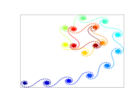
(a) The graph of a sum

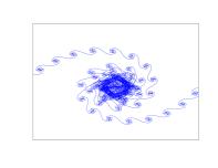
(b) A zoom of a detail of this graph

Figure 2. The graph of an exponential sum

One distinctly sees the spiraling structure that were dubbed curlicues in [1]. These are seen for $N$ such that $a_{L(N)}$ is small; indeed, in this case, as formulas (3.9) and (3.10) show, up to a rescaling and possibly a shift, the graph of the exponential sum is obtained by sampling points on the graph of the Fresnel integral, the Cornu spiral. Thanks to formulas (3.9) and (3.10), one can compute all the geometric characteristics of the curlicues when $a_{L(N)}$ is small.
In Fig. 2(b), we zoomed in on one of the curlicues shown in Fig. 2(a). Now we see the curlicues from the “previous generation”. They are seen in the case where $a_{L-1}$ is small and can be explained by the asymptotic analysis of the $(L-1)$th term in (2.7).

4. Estimates on the exponential sums

Using Theorem 3.1, we now estimate $S(N,a,b)$ in terms of the sequences $(a_{l})_{l}$ and $(b_{l})_{l}$.
For $L\in{\mathbb{N}}$, define

(4.1) $$M(L,a,b)=\max_{N^{-}(L)\leq N\leq N^{+}(L)}\left|\frac{S(N,a,b)}{\sqrt{N}}\right|$$

We prove

Proposition 4.1.

There exist positive constants $c$ and $C$ independent of $a$, and $b$ such that, for $L\in{\mathbb{N}}$,

(4.2) $$M(L,a,b)\leq C\,\frac{1}{\sqrt{|b_{L}|}+\sqrt[4]{a_{L}}},\\$$

and

(4.3) $$\text{if \ }\sqrt{|b_{l}|}+\sqrt[4]{a_{L}}\leq c,\text{ \ then \ }\frac{1}{C}\,\frac{1}{\sqrt{|b_{L}|}+\sqrt[4]{a_{L}}}\leq M(L,a,b)$$

where $a_{L}$ and $b_{L}$ are defined by (2.4) and (2.5).

Proof of Proposition 4.1.

Preliminaries.  Below, we consider only $N$ satisfying $N^{-}(L)\leq N\leq N^{+}(L)$. All the constants $C$ in the proof are independent of $L$, $N$, $a$ and $b$.
The analysis is based on Corollary 3.1. To obtain (4.2) from Corollary 3.1, we systematically use three simple estimates

(4.4) $$\forall x,y\in{\mathbb{R}},\quad\left|\int_{x}^{y}e(-\tau^{2}/2)\,d\tau\right|\leq C,$$

(4.5) $$\forall x,y\in{\mathbb{R}},\quad\left|\int_{x}^{y}e(-\tau^{2}/2)\,d\tau\right|\leq|x-y|,$$

(4.6) $$\forall x>0,\quad\left|\int_{\pm\infty}^{\pm x}e(-\tau^{2}/2)\,d\tau\right|\leq\frac{C}{x},$$

To simplify the notations, we write $\xi=\xi_{L}(N)$. Recall that $|b_{L}|\leq 1/2$ and $a_{L}\leq\xi\leq 1$. Note that this implies that $-1/2\leq-b_{L}+\xi\leq 3/2$. First, we get upper bounds for $S(N,a,b)/\sqrt{N}$. Therefore, depending on the values of $\xi$ and $b_{L}$, we consider several cases.

• Let $-b_{L}+\xi\geq 1/2$. One has

  (4.7) $$\left|\frac{S(N,a,b)}{\sqrt{N}}\right|\leq C.$$

  If $\xi\geq 1/4$, this estimate follows from (3.18) and (4.4). If $\xi\leq 1/4$ then $-b_{L}\geq 1/4$ and $1-(\xi-b_{L})\geq 1/4$. We estimate both integrals in (3.18) using (4.6) to obtain $\left|\frac{S(N,a,b)}{\sqrt{N}}\right|\leq C\sqrt{a_{L}/\xi}$. Then, (3.8) yields (4.7).

• Let $-b_{L}+\xi\leq 1/2$. We now have to consider three sub-cases depending on the value of $b_{L}$. In all these cases, we base our analysis on (3.17). By (3.8) the terms $1+O(a_{L}/\xi)$ and $O(\sqrt{a_{l}/\xi})$ in this formula are bounded by a constant, and we only have to estimate the term $T=\left|\frac{1}{\sqrt{\xi}}\,\int_{-\frac{b_{L}}{\sqrt{a_{L}}}}^{\frac{\xi-b_{L}}{\sqrt{a_{L}}}}e(-\tau^{2}/2)\,d\tau\right|$.

  • When $-b_{L}\geq\sqrt{a_{L}}$, one has

    (4.8) $$T\leq\frac{C}{\sqrt{|b_{L}|}}.$$

    If $\xi\leq a_{L}/|b_{L}|$, one estimate the integral using (4.5), otherwise one uses (4.6). In both cases, this yields (4.8).

  • When $|b_{L}|\leq\sqrt{a_{L}}$, one has

    (4.9) $$T\leq\frac{C}{\sqrt[4]{a_{L}}}.$$

    For $\xi\leq\sqrt{a_{L}}$, one uses (4.5), otherwise one uses (4.4). This leads to (4.9).

  • When $-b_{L}\leq-\sqrt{a_{L}}$, one has

    (4.10) $$T\leq\frac{C}{\sqrt{|b_{L}|}}.$$

    If $\xi\geq b_{L}/2$, then (4.4) yields (4.10). If $\xi\leq a_{L}/b_{L}$, then we get (4.10) using (4.5). Now, assume that $\xi\leq b_{L}/2$, and that $\xi\geq a_{L}/b_{L}$. The first inequality then implies that $-b_{L}+\xi\leq-b_{L}/2$, and, by means of (4.6), we get $T\leq C\,(\sqrt{a_{l}/\xi})/b_{L}$. As $\xi\geq a_{L}/b_{L}$, this implies (4.10).

Estimates (4.7) — (4.10) all imply the upper bound (4.2).

To prove the lower bound, we consider the leading term in the representations given in Corollary 3.1 for well chosen values of $\xi$. We consider three cases depending on the value of $b_{L}$.

• When $-b_{L}\leq-\sqrt{a_{L}}$. Recall that the possible values $\xi$ are described in Lemma 3.2. Let $\xi_{0}=\frac{a_{L}}{2b_{L}}$ and choose $N$ so that $|\xi-\xi_{0}|\leq a_{L}$. Then, one has

  $$-b_{L}+\xi\leq-\sqrt{a_{L}}+\sqrt{a_{L}}/2+a_{L}<a_{L}/2<1/2,$$

  and we can use (3.17).
  Let $t=b_{L}/\sqrt{a_{L}}$ and $s=\xi/\xi_{0}\in[1-2b_{L},1+2b_{L}]$. Assuming that $c$ in (4.3) is smaller than $1/16$, we get $s\in[1/2,3/2]$.
  Represent the leading term in (3.17) in the form $(b_{L})^{-1/2}g(t,s)$ where

  $$g(t,s)=\sqrt{\frac{2}{s}}\,t\,\int_{-t}^{-t+\frac{s}{2t}}e(-\tau^{2}/2)\,d\tau.$$

  Note that:

  1. $g$ never vanishes as the Cornu spiral i.e. the graph of the Fresnel integral $x\to\int_{-\infty}^{x}e(-\tau^{2}/2)\,d\tau$, $x\in{\mathbb{R}}$, has no self-intersections,

  2. $|g(t,s)|\to\frac{1}{\pi}\sqrt{\frac{2}{s}}sin(\pi s/2)$ as $t\to\infty$ uniformly in $s$; one checks this by integration by parts.

  Hence, for any $s$, $\displaystyle\inf_{t\geq 1}|g(t,s)|\geq C>0$. This implies that the leading term in (3.17) is bounded away from $0$ by $C/\sqrt{b_{L}}$. On the other hand, for $\xi=s\xi_{0}$, the error term in (3.17) is bounded by $C\sqrt{b_{L}}$. So, if $\sqrt{b_{L}}<c$, and $c$ is small enough, we see that the right hand side in  (3.17) is bounded away from $0$ by $C/\sqrt{b_{L}}$. This completes the proof of (4.3) in the case where $-b_{L}\leq-\sqrt{a_{L}}$.

• When $-b_{L}\geq\sqrt{a_{L}}$. One proves the lower bound almost in the same way as in the previous case. Now, we define $\xi_{0}=\frac{a_{L}}{2|b_{L}|}$ and choose $N$ as before. We get $-b_{L}+\xi\leq|b_{L}|+\sqrt{a_{L}}/2+a_{L}$, and the last expression is smaller than $1/2$ if $c$ in (4.3) is chosen small enough.
  We define $s$ as above and let $t=|b_{L}|/\sqrt{a_{L}}$. Hence, $s\in[1/2,3/2]$ and $t\geq 1$. Then, we write the leading term in (3.17) as $|b_{L}|^{-1/2}g(t,s)$ where

  $$g(t,s)=\sqrt{\frac{2}{s}}\,t\,\int_{t}^{t+\frac{s}{2t}}e(-\tau^{2}/2)\,d\tau.$$

  The analysis is then analogous to the one done in the previous case; we omit further details.

• When $|b_{L}|\leq\sqrt{a_{L}}$. The plan of the proof remains the same as in the previous cases. Now, we define $\xi_{0}=\sqrt{a_{L}}$. The number $N$ is chosen as before. We get $-b_{L}+\xi\leq 2\sqrt{a_{L}}+a_{L}$, and so this expression is smaller than $1/2$ if $c$ in (4.3) is chosen small enough.
  We define $s$ as before, and we let $t=b_{L}/\sqrt{a_{L}}$. We get $|t|\leq 1$ and $s\in[1/2,3/2]$ (if $c$ is chosen small enough). The leading term in (3.17) is equal to $(a_{L})^{-1/4}g(t,s)$, with

  $$g(t,s)=\sqrt{\frac{1}{s}}\,\int_{-t}^{-t+s}e(-\tau^{2}/2)\,d\tau.$$

  Again $g\neq 0$, and so, on the compact set $(t,s)\in[-1,1]\times[1/2,3/2]$, the factor $g$ is bounded away from $0$ by a constant $C$. Now, representation (3.17) implies that

  $$|S(N,a,b)|\geq C/\sqrt[4]{a_{L}}-C\sqrt[4]{a_{L}}$$

  (if $c$ is chosen small enough), and we obtain (4.3).

This completes the proof of the lower bound and, so, the proof of Proposition 4.1. ∎

5. The proof of Theorem 0.1

We now turn the proofs of Theorem 0.1 and Theorem 0.2 in the next section. Both will be deduced from Proposition 4.1 and the study of certain dynamical systems.

5.1. Reduction of the proof of Theorem 0.1 to the analysis of a dynamical system

We first reduce the proof of Theorem 0.1 to the proof of two lemmas describing properties of the dynamical system defined on the square $K:=[0,1)\times(-1/2,1/2]$ by the formulas (2.4) and (2.5). The idea of such a reduction was inspired to us by the proof of Theorem II, Chapter 7, from [2].
Note that it suffices to prove Theorem 0.1 in the case when

(5.1) $$\forall l\in{\mathbb{N}},\quad|g(l)|\leq 1/2,\quad\text{and}\quad\lim_{l\to\infty}g(l)=0$$

which we assume from now on.
We begin by formulating the two lemmas referred to above.

Let $\varphi:{\mathbb{R}}_{+}\to{\mathbb{R}}_{+}$ be a non increasing function. Let $\gamma(a,b)$ be the trajectory of the dynamical system defined by (2.4) and (2.5) that begins at $(a,b)\in K$. Let $\mathfrak{N}(L,a,b)$ be the number of the conditions

(5.2) $$\text{`` \ }\sqrt[4]{a_{l}}\leq\varphi(l)\quad\text{and}\quad\sqrt{|b_{l}|}\leq\varphi(l)\text{ \ ''}$$

with $0\leq l\leq L$ that are satisfied along $\gamma(a,b)$. Note that

(5.3) $$\mathfrak{N}(L,a,b)=\mathfrak{N}(L,\varphi,a,b)=\sum_{l=0}^{L}\chi(\sqrt[4]{a_{l}}\leq\varphi(l))\,\chi(\sqrt{|b_{l}|}\leq\varphi(l)),$$

where $\chi(\text{``statement''})$ is equal to 0 if the “statement” is false and is equal to 1 otherwise.
Let $m$ be the measure on $K$ defined by the formula $m(D)=\frac{1}{\ln 2}\,\int_{D}\frac{da\,db}{1+a}$ for $D\subset K$ measurable. Note that $m$ is a probability measure. We denote by $\|\mathfrak{N}(L,\cdot,\cdot)\|_{1}$ and $\|\mathfrak{N}(L,\cdot,\cdot)\|_{2}$, respectively, the $L^{1}(K,\,m)$ and $L^{2}(K,\,m)$ norms of the function $(a,b)\to\mathfrak{N}(L,a,b)$.

Remark 5.1.

The measure $\frac{1}{\ln 2}\frac{da}{1+a}$ is the invariant measure for the Gauss transformation $a\to\left\{\frac{1}{a}\right\}$ on $(0,1)$ (see [3]).

In what follows, $C$ denotes various positive constants that are independent of $L$, $a$ and $b$.
We prove

Lemma 5.1.

Let $\varphi:{\mathbb{R}}_{+}\to{\mathbb{R}}_{+}$ be a non increasing function such that, for all $l\in{\mathbb{N}}$, one has $\varphi(l)\leq 1/2$. Then,

(5.4) $$\|\mathfrak{N}(L,\varphi,\cdot,\cdot)\|_{1}\leq C\quad\forall L\in{\mathbb{N}}\quad\Longleftrightarrow\quad\sum_{N\geq 1}\varphi^{6}(N)<\infty.$$

and

Lemma 5.2.

Let $\varphi:{\mathbb{R}}_{+}\to{\mathbb{R}}_{+}$ be a non increasing function satisfying (5.1). If $\sum_{N\geq 1}\varphi^{6}(N)$ diverges, then, for all $L\in{\mathbb{N}}$,

$$\|\mathfrak{N}(L,\varphi,\cdot,\cdot)\|_{2}=(1+\delta(L))\,\|\mathfrak{N}(L,\cdot,\cdot)\|_{1}\,$$

with $\delta(L)\to 0$ as $L\to\infty$.

We prove these two lemmas in the sections 5.2, 5.3 and 5.4. We now use them derive Theorem 0.1.

5.1.1. The proof of the implication “$\Longleftarrow$” in (0.2)

In this part of the proof, we choose $\varphi(l)=g(l)$.
Note that $\displaystyle\|\mathfrak{N}(L,\cdot,\cdot)\|_{1}=\sum_{l=0}^{L}m(K_{l})$ where

$$K_{l}=\{(a,b);\ \sqrt[4]{a_{l}}\leq\varphi(l)\text{ and }\sqrt{|b_{l}|}\leq\varphi(l)\}.$$

Therefore, Lemma 5.1 implies that $\displaystyle\sum_{l=0}^{\infty}m(K_{l})<\infty$. Therefore, by the Borel-Cantelli lemma, for almost all $(a,b)\in K$, only a finite number of the conditions (5.2) is satisfied along $\gamma(a,b)$. Denote the set of such “good” $(a,b)$ by $G$.
Now, pick $(a,b)\in G$. Let $L_{0}\in{\mathbb{N}}$ be large enough so that either $\sqrt[4]{a_{l}}\geq g(l)$ or $\sqrt{|b_{l}|}\geq g(l)$ for all $l\geq L_{0}$. Pick an $L\geq L_{0}$. Using Proposition 4.1, we get

$$\max_{N^{-}(L)\leq N\leq N^{+}(L)}g(\ln N)\,\frac{|S(N,a,b)|}{\sqrt{N}}\leq C\frac{g(\ln N^{-}(L))}{g(L)}$$

as $g$ is a non increasing function. And now, as $g$ is a non increasing function, the implication “$\Longleftarrow$” follows from

Lemma 5.3.

For almost all $0<a<1$, when $L\to\infty$, one has

$$\ln N^{\pm}(L)=L(A+o(1))$$

where

(5.5) $$A=\frac{1}{\ln 2}\int_{0}^{1}\frac{\ln(1/a)\,da}{1+a}>1.$$

Proof of Lemma 5.3.

Let $a\not\in{\mathbb{Q}}$. Lemma 3.1 implies that

$$\frac{\ln(N^{-}(L))}{L}=\frac{1}{L}\,\sum_{l=0}^{L-1}\ln(1/a_{l})\,\,+O(1/L),\quad L\to\infty.$$

Recall that the Gauss map $a\to\{1/a\}$ on $(0,1)$ is ergodic, and that its invariant measure is $\frac{da}{\ln 2\,(1+a)}$ (see [3]). Therefore, by the Birkhoff-Khinchin Ergodic Theorem ([3]), for almost all $a\in(0,1)$, the limit $\displaystyle\lim_{L\to\infty}\frac{1}{L}\,\sum_{l=0}^{L-1}\ln(1/a_{l})$ exists and is equal to $A$ defined in (5.5). This completes the proof of the asymptotics of $\ln N^{-}$.
Integrating by parts, we get

$$A=\frac{1}{\ln 2}\int_{0}^{1}\frac{\ln(1+a)}{a}da\geq\frac{1}{\ln 2}\int_{0}^{1}\left(1-\frac{a}{2}\right)da=\frac{3}{4\ln 2}>1.$$

Finally, the asymptotics of $N^{+}$ follows from (3.2) and the asymptotics of $N^{-}$. This completes the proof of Lemma 5.3. ∎

This completes the proof of the implication “$\Longleftarrow$” in (0.2).

5.1.2. The proof of the implication “$\Longrightarrow$” in (0.2)

It suffices to prove that, for almost all $(a,b)\in K$, one has

(5.6) $$\sum_{N\geq 1}g^{6}(N)=+\infty\Longrightarrow\limsup_{N\to+\infty}\left(g(\ln N)\,\frac{|S(N,a,b)\,|}{\sqrt{N}}\right)=+\infty.$$

Let $A$ be the constant defined in (5.5). We choose $\varphi:{\mathbb{R}}_{+}\to{\mathbb{R}}_{+}$ so that

• $\displaystyle\sum_{l=1}^{\infty}\varphi^{6}(l)=+\infty$;

• $r(x):=\varphi(x)/g(2Ax)$ be a monotonously decreasing function;

• $\displaystyle\lim_{x\to\infty}r(x)=0$;

• $\varphi(x)\leq 1/2$.

Remark 5.2.

The third and the forth conditions guarantee that $\varphi$ satisfies the conditions (5.1).

The existence of such a function $\varphi$ follows from

Lemma 5.4.

Let $f:[0,+\infty)\to{\mathbb{R}}_{+}$ be a non increasing function such that $\displaystyle\sum_{l=1}^{\infty}f(l)=+\infty$. Then,

• for any $C>0$, one has $\displaystyle\sum_{l=1}^{\infty}f(Cl)=+\infty$.

• there exists $u:\,[1,+\infty)\to[0,1]$, a monotonously decreasing function, such that $\displaystyle\lim_{l\to\infty}u(l)=0$ and the series $\displaystyle\sum_{l=1}^{\infty}u(l)f(l)$ diverges.

Proof of Lemma 5.4.

The first statement follows from the fact that for any positive valued monotonously non increasing function the series $\displaystyle\sum_{l=1}^{\infty}f(l)$ and the integral $\displaystyle\int_{1}^{\infty}f(x)dx$ diverge simultaneously.
To prove the second statement, we pick $0<\alpha<1$ and define

$$u(x)=\alpha\,\left(\int_{0}^{x}f(x)\,dx\right)^{\alpha-1}.$$

Clearly, $u:\ [1,+\infty)\to{\mathbb{R}}_{+}$ is monotonously decreasing, and $u(x)$ tends to zero as $x$ tends to infinity. Furthermore, one has $\displaystyle\int_{1}^{+\infty}u(x)f(x)dx=+\infty$. Finally, to satisfy the condition $u(x)\leq 1$, it suffices to choose the constant $\alpha$ small enough. This completes the proof of the second statement.
The proof of Lemma 5.4 is complete. ∎

Using Lemmas 5.1 and 5.2, we now prove

Lemma 5.5.

There exists a set $B\subset K$ such that $m(B)=1$, and that, for all $(a,b)\in B$, there is an infinite sub-sequence of conditions (5.2) that are satisfied along $\gamma(a,b)$.

Proof.

We shall use the

Lemma 5.6.

Let $K$ be as defined above. Let $\mu$ be a probability measure on $K$ and pick $f:K\to{\mathbb{R}}_{+}$. Assume that, for some positive constant $c$, one has

$$c\|f\|_{L^{2}(K,\mu)}\leq\|f\|_{L^{1}(K,\mu)}.$$

Then, for any $0<d<c$, one has

$$\mu\left(\,(x,y)\in K\,:\,\,f(x,y)>d\,\|f\|_{2}\right)\geq(c-d)^{2}.$$

This actually is a version of the Zygmund-Polya Lemma. When $\mu$ is the Lebesgue measure, its proof can be found for example in [2] (Lemma 2, chapter 7). The same proof works in our case.
Pick $\varepsilon\in(0,1/2)$. By Lemma 5.2, for sufficiently large $L$, we get

$$(1-\varepsilon)\|\mathfrak{N}(L,\cdot,\cdot)\|_{2}\leq\|\mathfrak{N}(L,\cdot,\cdot)\|_{1}.$$

For such $L$, by Lemma 5.6, one has

$$m\left(\{(a,b)\in K\,:\,\,\mathfrak{N}(L,a,b)>\varepsilon\,\|\mathfrak{N}(L,\cdot,\cdot)\|_{1}\}\right)\geq(1-2\varepsilon)^{2}.$$

In view of Lemma 5.1, this implies that the measure of the set of $(a,b)$ for which $\mathfrak{N}(L,a,b)\to+\infty$ as $L\to\infty$ is bounded from below by $1-2\varepsilon$. As $\varepsilon>0$ can be taken arbitrarily small, this proves Lemma 5.5. ∎

Now, pick $(a,b)\in B$. There are infinitely many $l$ for which condition (5.2) is satisfied along $\gamma(a,b)$. Assume that $L$ is one of them. Using Proposition 4.1, as $g$ is non increasing, we get

$$\max_{N^{-}(L)\leq N\leq N^{+}(L)}g(\ln N)\,\frac{|S(N,a,b)|}{\sqrt{N}}\geq C\frac{g(\ln N^{+}(L))}{\varphi(L)}.$$

Combined with Lemma 5.3, this implies that, for $L$ sufficiently large,

$$\max_{N^{-}(L)\leq N\leq N^{+}(L)}g(\ln N)\,\frac{|S(N,a,b)|}{\sqrt{N}}\geq C\frac{g(2AL)}{\varphi(L)}.$$

For our choice of $\varphi$, the right hand side is equal to $1/r(L)$, and so, tends to $+\infty$ as $L\to\infty$. This yields (5.6) and completes the proof of Theorem 0.1.∎

5.2. Analysis of the dynamical system: an invariant family of densities

Let $(a_{L},b_{L})$ be related to $(a,b)$ by (2.4) and (2.5). In the next subsections, for a fixed $a$, we study integrals of the form $\int_{-1/2}^{1/2}g(b_{L}(a,b))\,f(b)\,db$, where $f(\cdot)$ is considered as a density of a measure. We change the variable $b$ to $b_{L}$ to get

$$\int_{-1/2}^{1/2}g(b_{L})\,f(b)\,db=\int_{-1/2}^{1/2}g(b_{L})(P_{a_{L-1}}\dots P_{a_{1}}P_{a}f)(b_{L})db_{L},$$

where

(5.7) $$\begin{split}(P_{a_{l}}f)(b)=a_{l}\sum_{m\in{\mathbb{Z}}\,:\,-1/2<b(m)\leq 1/2}f(b(m))\\ \text{and }\quad b(m):=a_{l}\,(-b+[1/a_{l}]/2+m).\end{split}$$

The operator $P_{a_{l}}$ is the Perron-Frobenius operator of the map acting on $(-1/2,1/2]$ defined in (2.5). In the present section, we describe a family of densities $f(\cdot)$ invariant under the cocycle $(a,f(\cdot))\mapsto(\{1/a\},\,P_{a}f(x,\cdot))$ and study properties of this family.
Fix $0<a<1$ and pick $A\geq 0$, $B\geq 0$ such that

(5.8) $$aA+(1-a)B=1.$$

The function

(5.9) $$f(b\,|\,a,A,B)=\left\{\begin{array}[]{ll}A,&\text{ if }|b|<a/2\\ B,&\text{ if }|b|>a/2\end{array}\right.$$

is the density of a probability measure on $(-1/2,1/2]$.
Our central observation is

Theorem 5.1.

Fix $a\in(0,1)$ and choose $A$ and $B$ as above. Then

(5.10) $$P_{a}f(\cdot\,|\,a,A,B)=f(\cdot\,|\,a_{1},A_{1},B_{1}),$$

where $a_{1}$ is related to $a$ by (2.1), and

(5.11) $$\begin{pmatrix}A_{1}\\ B_{1}\end{pmatrix}=S(a)\,\begin{pmatrix}A\\ B\end{pmatrix},\quad S(a)=\begin{pmatrix}a&1-aa_{1}\\ a&1-a-aa_{1}\end{pmatrix}.$$

In addition, one has

(5.12) $$a_{1}A_{1}+(1-a_{1})B_{1}=aA+(1-a)B=1.$$

Proof.

Represent $a$ in the form $a=\frac{1}{N+a_{1}}$ where $N=[1/a]$ and $a_{1}=\{1/a\}$. Assume that $N$ is even, i.e.,

(5.13) $$a=\frac{1}{2n+a_{1}},\quad\quad n\in{\mathbb{N}},\quad 0\leq a_{1}<1.$$

Then, the general formula (5.7) can be rewritten in the form

(5.14) $$(P_{a}f)(b)=a\,\cdot\,\left\{\begin{array}[]{ll}\displaystyle\sum_{m=-n+1}^{n}f((m-b)a),&\text{ if }b>a_{1}/2,\\ \displaystyle\sum_{m=-n}^{n}f((m-b)a),&\text{ if }|b|\leq a_{1}/2,\\ \displaystyle\sum_{m=-n}^{n-1}f((m-b)a),&\text{ if }b<-a_{1}/2.\end{array}\right.$$

So, applying $P_{a}$ to $f(\cdot\,|\,a,A,B)$, and assuming that $a_{1}/2<b_{1}<1/2$, we get

$$(P_{a}f(\cdot\,|\,a,A,B))(b_{1}) =a\,\left(\displaystyle\sum_{m=1}^{n}f((m-b_{1})a|a,A,B)\right.$$

$$+f(-b_{1}a|a,A,B)+\left.\displaystyle\sum_{m=-n+1}^{-1}f((m-b_{1})a|a,A,B)\right)$$

$$=a(nB+A+(n-1)B)=a(A+(2n-1)B)$$

$$\hskip 14.22636pt=aA+(1-a-aa_{1})B$$

as $0<a<1$.
As $f(.|a,A,B)$ is even, we get the same result for $-1/2<b_{1}<-a_{1}/2$. In the same way as above, we compute $(P_{a}f(\cdot\,|\,a,A,B)(a,b_{1})=aA+(1-aa_{1})B$ for $|b_{1}|<a_{1}/2$.
The thus obtained formulas imply (5.10) and (5.11) when $[1/a]$ is even.
The case of odd $[1/a]$ is treated analogously to the case of even $[1/a]$.
Finally, using (5.11), we get

$$a_{1}A_{1}+(1-a_{1})B_{1} =a_{1}(aA+(1-aa_{1})B)$$

$$\hskip 56.9055pt+(1-a_{1})(aA+(1-a-aa_{1})B)$$

$$=aA+(1-a)B$$

which proves (5.12) as $A$ and $B$ satisfy (5.8). This completes the proof of Theorem 5.1. ∎

We now analyze the properties of the transformation (5.11). Let $a\in(0,1)\setminus{\mathbb{Q}}$. Consider the sequence $a_{0},a_{1},a_{2},\,\dots$ defined by (2.4). We prove

Lemma 5.7.

Pick $l>1$. One has

$$P_{a_{l-1}}P_{a_{l-2}}\dots P_{a_{1}}P_{a}f(\cdot\,|\,a,A,B)=f(\cdot\,|\,a_{l},A_{l},B_{l}),$$

where

(5.15) $$B_{l}=1-\sum_{m=0}^{l-2}(-1)^{m}\prod_{n=l-m}^{l}a_{n}a_{n-1}+(-1)^{l}\prod_{n=1}^{l}a_{n}a_{n-1}\,B,$$

(5.16) $$A_{l}=B_{l}+a_{l-1}B_{l-1}.$$

Proof.

Let $A_{0}=A$ and $B_{0}=B$. By Theorem 5.1, for $l\in{\mathbb{N}}$,

(5.17) $$A_{l}=a_{l-1}A_{l-1}+(1-a_{l-1}a_{l})B_{l-1},$$

(5.18) $$B_{l}=a_{l-1}A_{l-1}+(1-a_{l-1}-a_{l}a_{l-1})B_{l-1}.$$

Subtracting (5.18) from (5.17), we prove (5.16). Furthermore, substituting into (5.18) with $l$ replaced by $l+1$ the value of $A_{l}$ given by (5.16), we get

$$B_{l+1}=(1-a_{l+1}a_{l})B_{l}+a_{l}a_{l-1}B_{l-1},\quad\forall l\in{\mathbb{N}}.$$

This implies that

$$B_{l+1}+a_{l+1}a_{l}B_{l}=B_{l}+a_{l}a_{l-1}B_{l-1},\quad\forall l\in{\mathbb{N}}.$$

Now, for $l=1$, equation (5.18) implies that

$$B_{1}+a_{1}a_{0}B_{0}=aA_{0}+(1-a)B_{0}=1.$$

This formula and the previous equation for $\{B_{l}\}_{l\in{\mathbb{N}}}$ imply that

$$B_{l}=1-a_{l}a_{l-1}B_{l-1},\quad\forall l\in{\mathbb{N}}.$$

This relation allows to express $B_{l}$ directly in terms of $B_{0}=B$, and one obtains (5.15). This completes the proof of Lemma 5.7. ∎

To complete this section, we discuss another family of densities $f(\cdot\,|\,a,M)$, $M\in{\mathbb{N}}$, such that $P_{a}f(\cdot\,|\,a,M)=f(\cdot\,|\,a_{1},A,B)$. We prove

Lemma 5.8.

For $a\in(0,1)$ and $M\in{\mathbb{N}}$ satisfying,

(5.19) $$M\leq\left\{\begin{array}[]{ll}\frac{1}{2}\,\left[\frac{1}{a}\right]&\text{ if }[1/a]\text{ is even,}\\ \\ \frac{1}{2}\,\left[\frac{1}{a}+1\right]&\text{ if }[1/a]\text{ is odd.}\end{array}\right.$$

Let

(5.20) $$f(b|a,M)=\left\{\begin{array}[]{ll}\displaystyle\frac{\chi(\,|b|\leq a(M-a_{1}/2)\,)}{a(2M-a_{1})}&\text{ if }[1/a]\text{ is even,}\\ \\ \displaystyle\frac{\chi(\,|b|\leq a(M-1/2-a_{1}/2)\,)}{a(2M-1-a_{1})}&\text{ if }[1/a]\text{ is odd.}\end{array}\right.$$

Then,

(5.21) $$P_{a}f(\cdot\,|a,M)=f(\cdot\,|a_{1},A_{1},B_{1}),$$

and

(5.22) $$\text{if }M>1,\text{ then }A_{1},B_{1}=1+O(1/M),$$

the error estimate being uniform in $a$.

Proof.

Assume that $[1/a]$ is even. In the sums in the right hand side of (5.14), only the terms with $-M+a_{1}/2+b_{1}\leq m\leq M-a_{1}/2+b_{1}$ are non zero. So, for $a_{1}/2<b_{1}<1/2$, we get

$$\begin{split}(P_{a}f(\cdot\,|\,a,M))(b_{1})&=a\,\displaystyle\sum_{m=-M+1}^{M}f((m-b_{1})a|a,M)\\ &=\frac{2M}{2M-a_{1}}=1+\frac{a_{1}}{2M-a_{1}}.\end{split}$$

And, for $0<b_{1}<a_{1}/2$, we obtain

$$\begin{split}(P_{a}f(\cdot\,|\,a,M))(a,b_{1})&=a\,\displaystyle\sum_{m=-M+1}^{M-1}f((m-b_{1})a|a,M)\\ &=\frac{2M-1}{2M-a_{1}}=1-\frac{1-a_{1}}{2M-a_{1}}.\end{split}$$

In the case of negative $b_{1}$, we obtain the same formulas as for $-b_{1}$. This implies (5.21) with

$$A_{1}=1-\frac{1-a_{1}}{2M-a_{1}}\quad\text{ and }\quad B_{1}=1+\frac{a_{1}}{2M-a_{1}}.$$

As $0<a_{1}<1$ and $M\geq 1$, we see that $A_{1},B_{1}=1+O(1/M)$.
This completes the proof of Lemma 5.8 for $[1/a]$ even. To complete the proof of Lemma 5.8, the case of odd $[1/a]$ is treated similarly. ∎

5.3. Proof of Lemma 5.1

By (5.3),

(5.23) $$\|\mathfrak{N}(L,\cdot,\cdot)\|_{1}=\sum_{l=0}^{L}\int_{K}\chi(a_{l}\leq\varphi^{4}(l))\,\chi(b_{l}\leq\varphi^{2}(l))\,\frac{da\,db}{\ln 2\,(1+a)},$$

where $(a_{l},b_{l})$ are related to $(a,b)$ by (2.4) and (2.5). To transform the right hand side of (5.23), we first use Fubini’s theorem and then, for fixed $a$, we perform the change of variable $b\to b_{l}$. As $f(b|a,1,1)=1$, Lemma 5.7 implies that

(5.24) $$\|\mathfrak{N}(L,\cdot,\cdot)\|_{1}=\frac{1}{\ln 2}\sum_{l=0}^{L}\int_{0}^{1}\frac{\chi(a_{l}\leq\varphi^{4}(l))\cdot I(l)\,da}{1+a},$$

where

$$I(l):=\int_{-1/2}^{1/2}\chi(|b_{l}|\leq\varphi^{2}(l))\,f(b_{l}|a_{l},A_{l},B_{l})\,db_{l},$$

the coefficients $A_{l}$ and $B_{l}$ being defined by (5.16) and (5.15) with $B_{0}=1$.
Recall that $\varphi_{l}<1/2$.
Let us study $I(l)$ under the condition $a_{l}\leq\varphi^{4}(l)$. Using (5.9), we compute

(5.25) $$I(l) =2\left(A_{l}\int_{0}^{a_{l}/2}+B_{l}\int_{a_{l}/2}^{1/2}\right)\chi(b_{l}\leq\varphi^{2}(l))\,db_{l}$$

$$=(A_{l}\,a_{l}+B_{l}\,(2\varphi^{2}(l)-a_{l}))=(a_{l}\,a_{l-1}\,B_{l-1}+2B_{l}\,\varphi^{2}(l)),$$

where, in the second step, we used the inequalities $a_{l}/2\leq\varphi^{4}(l)/2<\varphi^{2}(l)$ and $\varphi^{2}(l)<1/2$ which follows from $\varphi(l)<1/2$, and, in the last step, we used (5.16).
Note that it follows from estimate (3.6) and formula (5.15) with $B_{0}=1$ that, for all $l\geq 0$, one has $1/2<B_{l}<1$. Therefore,

(5.26) $$\varphi^{2}(l)<2B_{l}\,\varphi^{2}(l)<I(l)<a_{l}+2\varphi^{2}(l)<3\varphi^{2}(l).$$

Let us now turn to the study of $\|\mathfrak{N}(L,\cdot,\cdot)\|_{1}$. As the density $\frac{1}{\ln 2\,(1+a)}$ is invariant with respect to the Gauss transformation $a\to\{1/a\}$, one computes

(5.27) $$\int_{0}^{1}\frac{\chi(a_{l}\leq\varphi^{4}(l))\,da}{1+a}=\int_{0}^{1}\frac{\chi(a_{l}\leq\varphi^{4}(l))\,da_{l}}{1+a_{l}}=\ln(1+\varphi^{4}(l)).$$

The inequality (5.26) and the equality (5.27) imply that

$$\frac{1}{\ln 2}\sum_{l=0}^{L}\ln(1+\varphi^{4}(l))\varphi^{2}(l)\leq\|\mathfrak{N}(L,\cdot,\cdot)\|_{1}\leq\frac{3}{\ln 2}\sum_{l=0}^{L}\ln(1+\varphi^{4}(l))\varphi^{2}(l).$$

This implies (5.4), hence, completes the proof of Lemma 5.1. ∎

5.4. Proof of Lemma 5.2

We now assume that $\displaystyle\lim_{l\to\infty}\varphi(l)=0$. This enables us to get more precise estimates for $\|\mathfrak{N}(L,\cdot,\cdot)\|_{1}$ in subsection 5.4.1. In subsection 5.4.2, using these estimates, we approximate $\|\mathfrak{N}(L,\cdot,\cdot)\|_{2}$ with $\|\mathfrak{N}(L,\cdot,\cdot)\|_{1}$ and, thus, prove Lemma 5.2.
Below, $C$ denotes positive constants independent of $a,b,L$ and other variables (e.g., indices of summation). Moreover, when writing $f=O(g)$, we mean that $|f|\leq C|g|$.

5.4.1. Precise estimates for $\|\mathfrak{N}(L,\cdot,\cdot)\|_{1}$

Recall that, in formula (5.25), one has $a_{l}\leq\varphi^{4}(l)$ and $B_{l}$ is computed by (5.15) with $B=1$. Formula (5.15) with $B=1$ implies that $1/2<B_{m}<1$ for all $m$. Moreover, as $a_{l}\leq\varphi^{4}(l)$ and $\varphi(l)$ is small, we can write $B_{l}=1+O(\varphi^{4}(l))$. So, we replace (5.25) with

(5.28) $$I(l)=2\varphi^{2}(l)(1+O(\varphi^{2}(l))).$$

This and (5.23) imply that

(5.29) $$\|\mathfrak{N}(L,\cdot,\cdot)\|_{1}=\sum_{l=0}^{L}J(l)\text{ where }J(l)=\frac{2}{\ln 2}\varphi^{6}(l)\,(1+O(\varphi^{2}(l))).$$

That is the formula that we need to estimate $\|\mathfrak{N}(L,\cdot,\cdot)\|_{2}$.

5.4.2. Estimates for $\|\mathfrak{N}(L,\cdot,\cdot)\|_{2}$

Using (5.3), we get

(5.30) $$\begin{split}\|&\mathfrak{N}(L,\cdot,\cdot)\|^{2}_{2}=\|\mathfrak{N}(L,\cdot,\cdot)\|_{1}+\\ &+\frac{2}{\ln 2}\sum_{0\leq l<m\leq L}\int_{0}^{1}\frac{da}{1+a}\chi(a_{l}\leq\varphi^{4}(l))\chi(a_{m}\leq\varphi^{4}(m))\,I(l,m)\end{split}$$

where

(5.31) $$I(l,m)=\int_{-1/2}^{1/2}\chi(|b_{l}|\leq\varphi^{2}(l))\chi(|b_{m}|\leq\varphi^{2}(m))\,db.$$

The central ingredient for the proof of Lemma 5.2 is

Lemma 5.9.

Let $l<m$. If $a_{l}\leq\varphi^{4}(l)$ and $a_{m}\leq\varphi^{4}(m)$, then

(5.32) $$I(l,m)=4\varphi^{2}(l)\varphi^{2}(m)\left(1+O(\varphi^{2}(l))\right).$$

Proof.

The analysis of the integral $I(l,m)$ begins as the analysis of the integral $I(l)$ in the previous section, and one easily computes

$$\begin{split}I(l,m)&=\int_{-1/2}^{1/2}\chi(|b_{l}|\leq\varphi^{2}(l))\chi(|b_{m}|\leq\varphi^{2}(m))f(b_{l}|a_{l},A_{l},B_{l})db_{l}\\ &=\int_{|b_{l}|<\varphi^{2}(l)}\chi(|b_{m}|\leq\varphi^{2}(m))f(b_{l}|a_{l},A_{l},B_{l})db_{l}\\ &=\left(A_{l}\int_{|b_{l}|<a_{l}/2}+B_{l}\int_{a_{l}/2<|b_{l}|<\varphi^{2}(l)}\right)\,\chi(|b_{m}|\leq\varphi^{2}(m))db_{l},\end{split}$$

and

(5.33) $$I(l,m)=a_{l}a_{l-1}B_{l-1}I_{1}(l,m)+B_{l}I_{2}(l,m),$$

where $B_{l}$ and $A_{l}$ are computed by (5.15) with $B=1$, and we have set

$$I_{1}(l,m)=\frac{1}{a_{l}}\int_{|b_{l}|<a_{l}/2}\chi(|b_{m}|\leq\varphi^{2}(m))db_{l},$$

(5.34) $$I_{2}(l,m)=\int_{|b_{l}|<\varphi^{2}(l)}\chi(|b_{m}|\leq\varphi^{2}(m))db_{l}.$$

Estimate the integral $I_{1}(l,m)$. Therefore, we use Lemma 5.7 with the sequence $(a_{j})_{j\geq l}$ instead of the sequence $(a_{j})_{j\geq 0}$. We compute

$$\begin{split}I_{1}(l,m)&=\int_{-1/2}^{1/2}\chi(|b_{m}|\leq\varphi^{2}(m))f(b_{l}|a_{l},1/a_{l},0)\,db_{l}\\ &=\int_{-1/2}^{1/2}\chi(|b_{m}|\leq\varphi^{2}(m))f(b_{m}|a_{m},\tilde{A}_{m},\tilde{B}_{m})\,db_{m}\\ &=a_{m}(\tilde{A}_{m}-\tilde{B}_{m})+2\tilde{B}_{m}\varphi^{2}(m),\end{split}$$

where $\tilde{A}_{m}$ and $\tilde{B}_{m}$ are computed in terms of $\tilde{A}_{l}=1/a_{l}$ and $\tilde{B}_{l}=0$ by formulas (5.17) and (5.18). Formula (5.15) implies that $\tilde{B}_{m-1}\leq 1$, and $\tilde{B}_{m}=1+O(a_{m})$. These observations and (5.16) lead to the estimate

(5.35) $$I_{1}(l,m)=O(\varphi^{2}(m)).$$

To compute the integral $I_{2}(l,m)$, we use Lemma 5.8 with $a$ and $a_{1}$ replaced with $a_{l}$ and $a_{l+1}$.
Consider the case when $[1/a_{l}]$ is even. Choose an integer $M$ so that

(5.36) $$0\leq a_{l}(M-a_{l+1}/2)-\varphi^{2}(l)<a_{l}.$$

As $a_{l}\leq\varphi^{4}(l)$ and $\varphi(l)<1/2$, one has

(5.37) $$M\geq 1/\varphi^{2}(l)>4.$$

The definition of $I_{2}(l,m)$, (5.21) and (5.22) yield

$$\begin{split}I_{2}(l,m)&\leq\int_{|b_{l}|<a_{l}(M-a_{l+1}/2)}\chi(|b_{m}|\leq\varphi^{2}(m))\,db_{l}\\ &=2a_{l}(M-a_{l+1}/2)\int_{-1/2}^{1/2}\chi(|b_{m}|\leq\varphi^{2}(m))\,f(b_{l}|a_{l},M)\,db_{l}\\ &=2a_{l}(M-a_{l+1}/2)\int_{-1/2}^{1/2}\chi(|b_{m}|\leq\varphi^{2}(m))\,f(b_{l+1}|a_{l+1},A,B)\,db_{l+1}\end{split}$$

with $A,B=1+O(1/M)$. Moreover, in view of (5.37), one has

(5.38) $$A,B=1+O(1/M)=1+O(\varphi^{2}(l)).$$

If $m=1+l$, we compute

$$I_{2}(l,m)=2a_{l}(M-a_{m}/2)\,(a_{m}(A-B)+2B\varphi^{2}(m));$$

using (5.38) and (5.36), we finally obtain

(5.39) $$I_{2}(l,m)\leq 4\varphi^{2}(l)\varphi^{2}(m)\,(1+O(\varphi^{2}(l))).$$

If $m>l+1$, in the last integral for $I_{2}(l,m)$, we change the variable $b_{l+1}$ to $b_{m}$ and get

$$\begin{split}I_{2}(l,m)&\leq 2a_{l}(M-\frac{a_{l+1}}{2})\int_{-1/2}^{1/2}\chi(|b_{m}|\leq\varphi^{2}(m))\,f(b_{m}|a_{m},\tilde{\tilde{A}}_{m},\tilde{\tilde{B}}_{m})db_{l+1}\\ &=2a_{l}(M-a_{l+1}/2)\left(a_{m}(\tilde{\tilde{A}}_{m}-\tilde{\tilde{B}}_{m})+2\tilde{\tilde{B}}_{m}\varphi^{2}(m)\right)\end{split}$$

where $\tilde{\tilde{A}}_{m}$ and $\tilde{\tilde{B}}_{m}$ are obtained from $\tilde{\tilde{A}}_{l+1}=A$ and $\tilde{\tilde{B}}_{l+1}=B$ by formulas (5.17) and (5.18). Now, using (5.36) and Lemma 5.7 with $(a_{j})_{j\geq l+1}$ instead of $(a_{j})_{j\geq 0}$, as $l<m$ and $\varphi$ is non increasing, we get

(5.40) $$\begin{split}I_{2}(l,m)&\leq 4\varphi^{2}(l)\varphi^{2}(m)(1+O(\varphi^{2}(m))(1+O(\varphi^{2}(l)))\\ &\leq 4\varphi^{2}(l)\varphi^{2}(m)(1+O(\varphi^{2}(l))).\end{split}$$

We now complete the proof of Lemma 5.9. First, it follows from Lemma 5.7 that

(5.41) $$a_{l}=O(\varphi^{4}(l)),\quad B_{l-1}\leq 1\quad\text{and}\quad B_{l}=1+O(a_{l})=1+O(\varphi^{4}(l)).$$

We plug (5.35), (5.39) and (5.40) into (5.33). Taking into account (5.41), we obtain (5.32). This completes the proof of Lemma 5.9. ∎

We now return to the study of $\|\mathfrak{N}(L,\cdot,\cdot)\|_{2}$. Using well known properties of the Gauss map, we prove

Lemma 5.10.

One has

$$\|\mathfrak{N}(L,\cdot,\cdot)\|_{1}^{2}\leq\|\mathfrak{N}(L,\cdot,\cdot)\|_{2}^{2}\leq\|\mathfrak{N}(L,\cdot,\cdot)\|^{2}_{1}+\|\mathfrak{N}(L,\cdot,\cdot)\|_{1}+R_{L}$$

where, for some $C>0$, one has

$$R_{L}:=\displaystyle\sum_{m,l=0}^{L}\,\varphi^{6}(l)\varphi^{6}(m)\cdot O\left(\varphi^{2}(m)+\varphi^{2}(l)+e^{-(m-l)/C}\right).$$

Proof.

The lower bound on $\|\mathfrak{N}(L,\cdot,\cdot)\|_{2}^{2}$ is a consequence of the Cauchy-Schwarz inequality.
To prove the upper bound, we substitute (5.32) into (5.30) to get

(5.42) $$\|\mathfrak{N}(L,\cdot,\cdot)\|_{2}^{2}=\|\mathfrak{N}(L,\cdot,\cdot)\|_{1}\\ +8\sum_{0\leq l<m\leq L}\varphi^{2}(l)\varphi^{2}(m)\,P\left(\,a_{l}\leq\varphi^{4}(l),\,a_{m}\leq\varphi^{4}(m)\,\right)\left(1+O(\varphi^{2}(l))\right),$$

where we have defined

$$P(a_{l}\leq\alpha,a_{m}\leq\beta):=\frac{1}{\ln 2}\int_{0}^{1}\frac{da}{1+a}\chi(a_{l}\leq\alpha)\chi(a_{m}\leq\beta)$$

i.e. $P(a_{l}\leq\alpha,a_{m}\leq\beta)$ is the probability (with respect to the invariant measure of the Gauss map) that $a_{m}<\beta$ and $a_{l}<\alpha$. It is controlled by Gordin’s Theorem (see [7], Theorem 3 and remarks following this theorem). By Gordin’s Theorem, there exists two constants $A>0$ and $\lambda>0$ such that, for all $0\leq l<m<\infty$ and for any integer $\alpha>0$ and any real number $\beta>0$, one has

(5.43) $$|P(a_{l}\leq 1/\alpha,a_{m}\leq\beta)-P(a_{l}\leq 1/\alpha)P(a_{m}\leq\beta)|\\ \leq A\,P(a_{l}\leq 1/\alpha)\,P(a_{m}\leq\beta)\,e^{-\lambda(m-l)}$$

where we have defined

$$P(a_{l}\leq\alpha):=\frac{1}{\ln 2}\int_{0}^{1}\frac{da}{1+a}\chi(a_{l}\leq\alpha).$$

Now, choose a positive integer $s$ so that

$$\frac{1}{s+1}\leq\varphi^{4}(l)<\frac{1}{s}.$$

Note that, as $\varphi(l)<1/2$, such a positive integer exists, and that

(5.44) $$\frac{1}{s}-\varphi^{4}(l)=O(\varphi^{8}(l)).$$

Using (5.43), we get

$$\begin{split}P(\,a_{l}\leq\varphi^{4}(l),&\,a_{m}\leq\varphi^{4}(m)\,)\leq P(\,a_{l}\leq 1/s,\,a_{m}\leq\varphi^{4}(m)\,)\\ &\leq P(\,a_{l}\leq 1/s\,)\,P(\,a_{m}\leq\varphi^{4}(m)\,)(1+Ae^{-\lambda(m-l)}).\end{split}$$

Using the definition of the invariant measure, we obtain

$$\begin{split}P(\,a_{m}\leq\varphi^{4}(m)\,)&=P(a\leq\varphi^{4}(m))=\frac{1}{\ln 2}\int_{0}^{\varphi^{4}(m)}\frac{da}{1+a}\\ &=\frac{\ln(1+\varphi^{4}(m))}{\ln 2}=\frac{1}{\ln 2}\varphi^{4}(m)\,(1+O(\varphi^{4}(m))).\end{split}$$

In the same way, (5.44) yields

$$P(\,a_{l}\leq 1/s\,)=\frac{1}{s\,\ln 2}\,\,(1+O(1/s))=\frac{1}{\ln 2}\varphi^{4}(l)\,(1+O(\varphi^{4}(l))).$$

These two results imply that

$$P(a_{l}\leq\varphi^{4}(l),\ a_{m}\leq\varphi^{4}(m))\\ \leq\frac{1}{(\ln 2)^{2}}\,\varphi^{4}(l)\,\varphi^{4}(m)\left(1+O\left(\varphi^{4}(l)+\varphi^{4}(m)+Ae^{-\lambda(m-l)}\right)\right).$$

Combining this estimate and (5.42), recalling (5.29), we obtain the upper bound on $\|\mathfrak{N}(L,\cdot,\cdot)\|_{2}^{2}$ announced in Lemma 5.10. This completes the proof of Lemma 5.10. ∎

Now, we can complete the proof of Lemma 5.2 by means of elementary estimates. Recall that by assumption of Lemma 5.2, $\sum_{l=0}^{\infty}\varphi^{6}(l)$ diverges. By (5.29), this implies that $\displaystyle\|\mathfrak{N}(L,\cdot,\cdot)\|_{1}=\sum_{l=0}^{L}J(l)\to\infty$ as $L\to\infty$. So, to prove that $\|\mathfrak{N}(L,\cdot,\cdot)\|_{2}^{2}=\|\mathfrak{N}(L,\cdot,\cdot)\|_{1}^{2}(1+o(1))$ when $L\to\infty$, and, thus, to complete the proof of Lemma 5.2, it suffices to show that

(5.45) $$\lim_{L\to\infty}\frac{\sum_{l=0}^{L}J(l)\varphi^{2}(l)}{\sum_{l=0}^{L}J(l)}=0,$$

(5.46) $$\lim_{L\to\infty}\frac{\sum_{l,m=0}^{L}J(l)J(m)e^{-|l-m|/C}}{\left(\sum_{l,m=0}^{L}J(l)\right)^{2}}=0.$$

As $\varphi(l)\to 0$ and $\displaystyle\sum_{l=0}^{L}J(l)\to\infty$, (5.45) is a standard result of Cesaro convergence.
As $J(m)$ is bounded uniformly in $m$, (5.46) follows from

$$\frac{\sum_{l,m=0}^{L}J(l)J(m)e^{-|l-m|/C}}{\left(\sum_{l=0}^{L}J(l)\right)^{2}}\leq C\,\frac{\sum_{l=0}^{L}J(l)\sum_{m=0}^{L}e^{-|l-m|/C}}{\left(\sum_{l=0}^{L}J(l)\right)^{2}}\leq\frac{C}{\sum_{l=0}^{L}J(l)}.$$

This completes the proof of Lemma 5.2

6. The proof of Theorem 0.2

Let $g$ be as in Theorem 0.2. We first prove

Lemma 6.1.

Let $g:{\mathbb{R}}_{+}\to{\mathbb{R}}_{+}$ be a non increasing function such that

$$\sum_{N\geq 1}g^{4}(N)<\infty.$$

Then, for almost all $a\in(0,1)$ and for all $b\in(-1/2,1/2]$, one has

(6.1) $$\limsup_{N\to+\infty}\left(g(\ln N)\,\frac{|S(N,a,b)\,|}{\sqrt{N}}\right)<\infty.$$

Proof of Lemma 6.1.

As $\displaystyle\sum_{N\geq 1}g^{4}(N)<\infty$, Theorem 30 of [10] implies that, for almost all $a\in(0,1)$, there exists $L_{0}\in{\mathbb{N}}$ such that $a_{l}\geq g^{4}(l)$ for all $l\geq L_{0}$. Pick $L\geq L_{0}$. Using Proposition 4.1, we get

$$\max_{N^{-}(L)\leq N\leq N^{+}(L)}g(\ln N)\,\frac{|S(N,a,b)|}{\sqrt{N}}\leq C\frac{g(\ln N^{-}(L))}{g(L)}$$

as $g$ is a non increasing function. And now, as $g$ is a non increasing function, (6.1) follows from Lemma 5.3. This completes the proof of Lemma 6.1. ∎

Now, Theorem 0.2 follows from

Proposition 6.1.

Let $g:{\mathbb{N}}\to{\mathbb{R}}_{+}$ be a non increasing function such that

$$\sum_{N\geq 1}g^{4}(N)=\infty.$$

Then, for almost all $a\in(0,1)$ and all $b\in{\mathcal{B}}_{a}$, one has

$$\limsup_{N\to+\infty}\left(g(\ln N)\,\frac{|S(N,a,b)\,|}{\sqrt{N}}\right)=\infty.$$

Indeed, if $\sum_{N\geq 1}g^{4}(N)=\infty$, by Proposition 6.1, for almost all $a$, as ${\mathcal{B}}_{a}$ is dense in $(-1/2,1/2]$, the set

$$\tilde{\mathcal{B}}_{a}:=\left\{b\in(-1/2,1/2];\ \limsup_{N\to+\infty}\left(g(\ln N)\,\frac{|S(N,a,b)\,|}{\sqrt{N}}\right)=+\infty\right\}$$

is dense in $(-1/2,1/2]$. As $b\mapsto S(N,a,b)$ is continuous and as

$$\tilde{\mathcal{B}}_{a}=\bigcap_{K\geq 1}\bigcap_{M\geq 1}\bigcup_{N\geq M}\left\{b\in(-1/2,1/2];\ g(\ln N)\,\frac{|S(N,a,b)\,|}{\sqrt{N}}>K\right\},$$

$\tilde{\mathcal{B}}_{a}$ is a dense $G_{\delta}$-set. This completes the proof of Theorem 5.1 once Proposition 6.1 is proved.

6.1. Proof of Proposition 6.1

Proposition 6.1 follows from

Lemma 6.2.

For $(a_{0},b_{0})$, define the inductive sequence $(a_{n},b_{n})$ by formulas (2.4) and (2.5).
Then, for almost every $a$ and all $b\in\mathcal{B}_{a}$, there exists $j_{0}\geq 1$ such that, for $j\geq j_{0}$, one has

(6.2) $$b_{j}\in\left\{0,\frac{1}{2},-\frac{a_{j}}{2}\right\}.$$

and

Proposition 6.2.

Let $g:{\mathbb{N}}\to{\mathbb{R}}_{+}$ be a non increasing function such that

$$\sum_{N\geq 1}g^{4}(N)=\infty.$$

Then, for almost all $a\in(0,1)$ and $b\in\{0,1/2,-a/2\}$, one has

(6.3) $$\limsup_{N\to+\infty}\left(g(\ln N)\,\frac{|S(N,a,b)\,|}{\sqrt{N}}\right)=\infty.$$

Indeed, let $\mathcal{A}_{0}$ be the set of total measure of $a$’s defined by Lemma 6.2. For $p\in{\mathbb{N}}$, let $g_{p}:{\mathbb{R}}^{+}\to{\mathbb{R}}^{+}$ be the function $g_{p}(x)=g(x+p)$. If $\sum_{N\geq 1}g^{4}(N)=\infty$ then, for any $p\in{\mathbb{N}}$, one has $\sum_{N\geq 1}g_{p}^{4}(N)=\infty$. Let $\mathcal{A}^{p}$ be the set of total measure of $a$’s defined by Proposition 6.2 where the function $g$ is replaced by the function $g_{p}$.
If $G$ denotes the Gauss map (see (2.4)), the set $\displaystyle\mathcal{A}_{0}\cap\bigcap_{p,l\geq 0}G^{-l}(\mathcal{A}^{p})$ is of total measure. For $a$ in this set and $b\in\mathcal{B}_{a}$, there exists $j_{0}$ even such that (6.2) is satisfied and (6.3) is satisfied for $(a_{j_{0}},b_{j_{0}})$ and $g$ replaced by any $g_{p}$. Applying the renormalization formula (2.2) $j_{0}$ times, we see that

$$S(N,a,b)=C_{j_{0}}\,S(N_{j_{0}},a_{j_{0}},b_{j_{0}})+O(1)$$

where $\sqrt{a_{0}\cdots a_{j_{0}}}|C_{j_{0}}|=1$ and $N_{j_{0}}=N_{j_{0}}(N)$ is defined in (2.1) and satisfies $N_{j_{0}}\sim a_{0}\cdots a_{j_{0}}N$ when $N\to+\infty$. Hence

$$\frac{|S(N,a,b)\,|}{\sqrt{N}}\operatornamewithlimits{\sim}_{N\to+\infty}\frac{|S(N_{j_{0}},a_{j_{0}},b_{j_{0}})\,|}{\sqrt{N_{j_{0}}}}.$$

Moreover, for $p_{0}\geq|\ln\sqrt{a_{0}\cdots a_{j_{0}}}|+1$ and $N$ sufficiently large, one has $g_{p_{0}}(\ln N_{j_{0}}(N))\leq g(\ln N)$. Finally, noticing that when $N$ goes to $\infty$ running through all the integers, $N_{j_{0}}=N_{j_{0}}(N)$ does so too, we obtain

$$\limsup_{N\to+\infty}\left(g(\ln N)\,\frac{|S(N,a,b)\,|}{\sqrt{N}}\right)\geq\limsup_{N\to+\infty}\left(g_{p_{0}}(\ln N)\,\frac{|S(N,a_{j_{0}},b_{j_{0}})\,|}{\sqrt{N}}\right)=\infty.$$

So we have proved that Proposition 6.2 and Lemma 6.2 imply Proposition 6.1.
Proposition 6.2 is proved in section 6.2. We now turn to the proof of Lemma 6.2.

Proof of Lemma 6.2.

Pick $a=a_{0}\in(0,1)$ arbitrary and let $b_{0}\in{\mathcal{B}}_{a}$. One can represent $b_{0}$ as

$$b_{0}=\frac{1}{2}\,(n_{0}\,a_{0}-[n_{0}\,a_{0}]-\varepsilon_{0}),\quad n_{0}\in{\mathbb{Z}},\quad\varepsilon_{0}\in\{0,1\}.$$

Computing $b_{1}$ from $b_{0}$ by formula (2.1), one obtains

(6.4) $$b_{1}=\left\{\frac{1}{2}\,([n_{0}a_{0}]+\varepsilon_{0})\,a_{1}+\frac{1}{2}\,\left(([n_{0}a_{0}]+\varepsilon_{0}+1)\,\left[\frac{1}{a_{0}}\right]-n_{0}\right)\right\}_{0}.$$

Therefore,

$$b_{1}=b_{1}(b_{0})=\frac{1}{2}(n_{1}\,a_{1}-[n_{1}\,a_{1}]-\varepsilon_{1}),$$

$$n_{1}=[a_{0}\,n_{0}]+\varepsilon_{0},\quad\quad\varepsilon_{1}\in\{0,1\}.$$

Hence, we can define $(b_{j})_{j\geq 0}$ by formula (2.5) and represent it as above as

$$b_{j}=\frac{1}{2}\,(n_{j}\,a_{j}-[n_{j}\,a_{j}]-\varepsilon_{j}),$$

$$n_{j}=[a_{j-1}\,n_{j-1}]+\varepsilon_{j-1},\quad\varepsilon_{j}\in\{0,1\}.$$

Note that, if $n_{j-1}\in\{-1,0,1\}$ then $n_{j}\in\{-1,0,1\}$.

Let $\mathcal{Z}_{a}=\frac{1}{2}((2{\mathbb{Z}}+1)a+(2{\mathbb{Z}}+1))$. We note that (see (6.4))

$$b_{j+1}\in{\mathcal{Z}}_{a_{j+1}}\quad\Longleftrightarrow\quad b_{j}\in{\mathcal{Z}}_{a_{j}}.$$

So, for $b\in{\mathcal{B}}_{a}$, for any $j\geq 0$, $b_{j}\not\in{\mathcal{Z}}_{a_{j}}$.
Consider now the sequence $(\beta_{j})_{j\geq 0}$ defined by

$$\beta_{0}=|n_{0}|,\quad\beta_{j+1}=a_{j}\,\beta_{j}+1\text{ for }j\geq 0.$$

One checks that, for all $j\geq 0$, one has $-\beta_{j}\leq n_{j}\leq\beta_{j}$. Moreover, using (3.6), we get

$$0\leq\beta_{j}\leq 1+a_{j-1}\cdots a_{0}\,|n_{0}|+4a_{j-1},\quad j\geq 2.$$

Theorem 30 of [10] implies that, for almost every $a$, there exists a subsequence of $(a_{j})_{j}$ that tends to $0$. Therefore, we see that, for almost every $a$, for some $j_{0}$ sufficiently large, one has $n_{j_{0}}\in\{-1,0,1\}$. But then, for all $j\geq j_{0}$, $n_{j}\in\{-1,0,1\}$. As $b_{j}\not\in{\mathcal{Z}}_{a_{j}}$ $\forall j\geq 0$, the last observation implies that for almost any $a$ for all $j$ sufficiently large

$$b_{j}\in\left\{0,\frac{1}{2},\frac{a_{j}}{2},-\frac{a_{j}}{2}\right\}.$$

Consider the mapping $b\mapsto b_{1}$, defined by (2.1). We have

(6.5) $$\begin{split}b_{1}(0)=\begin{cases}0\text{ if }\left[\frac{1}{a_{0}}\right]\text{ is even}\\ \frac{1}{2}\text{ if }\left[\frac{1}{a_{0}}\right]\text{ is odd}\end{cases},\quad b_{1}\left(\frac{1}{2}\right)=-\frac{a_{1}}{2},\\ b_{1}\left(\frac{a_{0}}{2}\right)=b_{1}\left(-\frac{a_{0}}{2}\right)=\begin{cases}\frac{1}{2}\text{ if }\left[\frac{1}{a_{0}}\right]\text{ is even}\\ 0\text{ if }\left[\frac{1}{a_{0}}\right]\text{ is odd}\end{cases}.\end{split}$$

So, for almost all $a$, for all $j$ sufficiently large, one has $b_{j}\in\left\{0,1/2,-a_{j}/2\right\}$. This completes the proof of Lemma 6.2. ∎

6.2. Proof of Proposition 6.2

For given $(a_{0},b_{0})$, define the $(a_{n},b_{n})$ by formulas (2.4) and (2.5). Recall that for all $a_{0}\in(0,1)$ and all $b_{0}\in{\mathcal{B}}_{a_{0}}$, one has $b_{j}\in{\mathcal{B}}_{a_{j}}$ for all $j\geq 0$. To prove Proposition 6.2 it is sufficient to prove that, for almost every $(a_{0},b_{0})$, there are infinitely many $l$ such that $a_{l}\leq\varphi^{4}(l)$ and $b_{l}=0$. The arguments leading to this conclusion are analogous to the arguments from the end of the section 5.1.2 (just after the end of proof of Lemma 5.5). We omit the details and note only that now we pick $\varphi:{\mathbb{R}}_{+}\to{\mathbb{R}}_{+}$ so that

• $\displaystyle\sum_{l=1}^{\infty}\varphi^{4}(l)=+\infty$;

• $r(x):=\varphi(x)/g(2Ax)$ be a monotonously decreasing function;

• $\displaystyle\lim_{x\to\infty}r(x)=0$;

• $\varphi(x)\leq 1/2$;

where $A$ be the constant defined in (5.5).

As, for all $j\geq 0$, $b_{j}\in{\mathcal{B}}_{a_{j}}$, then to study the trajectories $\{(a_{j},b_{j})\subset{\mathbb{R}}^{2},\,j\geq 0\}$ it is possible and convenient to study trajectories of an one dimensional dynamical system defined by a piecewise monotonic map of a real interval. Let us describe this system. Consider the interval $X=[0,3]$ endowed with the probability measure $d\nu$ of density (with respect to the Lebesgue measure)

$$\nu(x)=\frac{1}{3\ln 2}\left(\sum_{i=0}^{2}\frac{1}{x-i+1}\mathbb{1}_{[i,i+1]}(x)\right)$$

i.e., up to the factor $1/3$, in each interval $[i,i+1]$, the measure $\nu$ is the invariant measure for the Gauss map “shifted” to this interval.
On $(X,d\nu)$, consider the dynamical system defined by the iterates of the map $\tilde{T}:\,\tilde{a}_{0}\mapsto\tilde{a}_{1}$ such that

• if $\tilde{a}_{0}\in[0,1]$ then

  $$\tilde{a}_{1}=\left\{\frac{1}{\tilde{a}_{0}}\right\}+\begin{cases}0&\text{ if }\left[\frac{1}{\tilde{a}_{0}}\right]\text{ if even},\\ 2&\text{ if }\left[\frac{1}{\tilde{a}_{0}}\right]\text{ is odd};\end{cases}$$

• if $\tilde{a}_{0}\in(1,2)$ then

  $$\tilde{a}_{1}=\left\{\frac{1}{\tilde{a}_{0}-1}\right\}+\begin{cases}2&\text{ if }\left[\frac{1}{\tilde{a}_{0}-1}\right]\text{ if even},\\ 0&\text{ if }\left[\frac{1}{\tilde{a}_{0}-1}\right]\text{ is odd};\end{cases}$$

• if $\tilde{a}_{0}\in(2,3)$ then

  $$\tilde{a}_{1}=\left\{\frac{1}{\tilde{a}_{0}-2}\right\}+1.$$

Clearly, for $b_{0}\in{\mathcal{B}}_{a_{0}}$, there is one-to-one correspondence between the trajectories $\{(a_{j},b_{j})\subset{\mathbb{R}}^{2},\,j\geq 0\}$ of the input dynamical system and the trajectories $\{\tilde{a}_{j}\subset{\mathbb{R}},\,j\geq 0\}$ of the newly defined one:

(6.6) $$a_{j}=\{\tilde{a}_{j}\},\quad\quad b_{j}=\begin{cases}0&\text{ if \ }\tilde{a}_{j}\in(0,1)\\ -a_{j}/2,&\text{ if \ }\tilde{a}_{j}\in(1,2)\\ 1/2,&\text{ if \ }\tilde{a}_{j}\in(2,3)\end{cases},\quad\quad j\geq 0.$$

The value of $b_{j}$ is coded by $[\tilde{a}_{j}]$.
Analogously to what was done in section 5, we define

(6.7) $$\mathfrak{N}(L,\tilde{a}_{0})=\sum_{l=0}^{L}\chi(\sqrt[4]{\tilde{a}_{l}}\leq\varphi(l)).$$

where $\chi(\text{``statement''})$ is equal to 0 if the “statement” is false and is equal to 1 otherwise. Recall that $\varphi(l)<1/2$. Therefore,

$$\mathfrak{N}(L,\tilde{a}_{0})=\sum_{l=0}^{L}\chi(\sqrt[4]{a_{l}}\leq\varphi(l))\,\chi(b_{l}=0).$$

So, if $\mathfrak{N}(L,\tilde{a}_{0})\to\infty$ as $L\to\infty$, then there are infinitely many $l$ such that $a_{l}\leq\varphi^{4}(l)$ and $b_{l}=0$.
The analysis of the counting function $\mathfrak{N}$ is similar to that done when proving Theorem 0.1. We will derive estimates for appropriate norms of the function $\mathfrak{N}$. Therefore, we will use the invariant measure and the exponential mixing of the dynamical system defined by $\tilde{T}$.
To prove the exponential mixing of the dynamical system defined by $\tilde{T}$, we use Theorem 3.1 of [11]. We check that $\tilde{T}$ defines a weighted covering system (Definition 3.5 of [11]). It suffices to prove

Lemma 6.3.

Let $P$ be the Perron-Frobenius operator of $\tilde{T}$.
For any $I\subset X$ non empty open interval, there exists $N=N(I)\in{\mathbb{N}}$ and $C=C(I)>0$ such that $P^{N}\mathbb{1}_{I}\geq C\,\mathbb{1}_{X}$.

Proof of Lemma 6.3.

Recall that the Perron-Frobenius operator is defined by the formula

(6.8) $$(Pu)(a_{1})=\nu^{-1}(a_{1})\,\sum_{a:\,\,\tilde{T}(a)=a_{1}}\frac{\nu(a)u(a)}{|\tilde{T}^{\prime}(a)|}.$$

Using the definitions of $\nu$ and $\tilde{T}$, we get

$$Pu=\left(P_{e}(u\mathbb{1}_{[0,1]})+P_{o}\tau_{1}(u\mathbb{1}_{[1,2]})\right)+\tau_{1}^{-1}(P_{e}+P_{o})\tau_{2}(u\mathbb{1}_{[2,3]})\\ +\tau_{2}^{-1}\,\left(P_{e}\tau_{1}(u\mathbb{1}_{[1,2]})+P_{o}(u\mathbb{1}_{[0,1]})\right).$$

where $\tau_{i}[u](x)=u(x+i)$ and the operators $P_{e}$ and $P_{o}$ are acting on $L^{1}([0,1])$ and defined as

$$(P_{e}u)(a)=(1+a)\sum_{k\geq 1}\frac{u\left((2k+a)^{-1}\right)}{(2k+a)(2k+1+a)}$$

$$(P_{o}u)(a)=(1+a)\sum_{k\geq 1}\frac{u\left((2k-1+a)^{-1}\right)}{(2k-1+a)(2k+a)}.$$

Note that $P_{e}+P_{o}$ is the Perron-Frobenius operator for the Gauss map on $([0,1],d\mu)$ where $d\mu$ is the invariant measure for the Gauss map.
Note that, there exists $c>0$ such that

• $P(\mathbb{1}_{[0,1]})\geq c\,(\mathbb{1}_{[0,1]}+\mathbb{1}_{[2,3]})$,

• $P(\mathbb{1}_{[1,2]})\geq c\,(\mathbb{1}_{[0,1]}+\mathbb{1}_{[2,3]})$

• $P(\mathbb{1}_{[2,3]})\geq c\,\mathbb{1}_{[1,2]}$.

Hence, one has $P^{3}(\mathbb{1}_{[i,i+1]})\geq c\,\mathbb{1}_{X}$ for $i\in\{0,1,2\}$. So, it suffices to show that for any interval $I$, there exists $i$, $N$ and $c$ so that $P^{N}\mathbb{1}_{I}\geq c\,\mathbb{1}_{[i,i+1]}$.
For $(n_{j})_{j\geq 1}$ integers, denote by $[n_{1},n_{2},\cdots,n_{p}]$ the real number defined by the continued fraction

$$[n_{1},n_{2},n_{3},\cdots,n_{p}]=\cfrac{1}{n_{1}+\cfrac{1}{n_{2}+\cfrac{1}{\ddots\cfrac{\ddots}{n_{p-1}+\cfrac{1}{n_{p}}}}}}.$$

Pick a non-empty open interval $I\subset[0,3]$. It contains an interval of the form $[x,x^{\prime}]$ where $x=i+[n_{1},\cdots,n_{p-1},n_{p}]$ and $x^{\prime}=i+[n_{1},\cdots,n_{p-1},n^{\prime}_{p}]$ for some $i\in\{0,1,2\}$ and $|n_{p}-n^{\prime}_{p}|=1$. So, it suffices to show Lemma 6.3 for intervals of that form.
Pick now $y=[n_{1},\cdots,n_{p-1},n_{p}]$ and $y^{\prime}=[n_{1},\cdots,n^{\prime}_{p}]$ where $|n_{p}-n^{\prime}_{p}|=1$. By the definition of the Gauss map, one obtains

$$P_{e}\mathbb{1}_{[y,y^{\prime}]}\geq c\mathbb{1}_{[\tilde{y}^{\prime},\tilde{y}]}\text{ if }n_{1}\text{ is even}\quad\text{and}\quad P_{o}\mathbb{1}_{[y,y^{\prime}]}\geq c\mathbb{1}_{[\tilde{y}^{\prime},\tilde{y}]}\text{ if }n_{1}\text{ is odd}$$

where $\tilde{y}=[n_{2},\cdots,n_{p}]$ and $\tilde{y}^{\prime}=[n_{2},\cdots,n^{\prime}_{p}]$.
Hence, for $[x,x^{\prime}]$ an interval as above, one gets $P\mathbb{1}_{[x,x^{\prime}]}\geq c\mathbb{1}_{i+[\tilde{y}^{\prime},\tilde{y}]}$, where $i$ is an index in $\{0,1,2\}$ that depends on $x$.
Applying this $p$ times, we get $\displaystyle P^{p}\mathbb{1}_{[x,x^{\prime}]}\geq c\mathbb{1}_{[i,i+1]}$ for some $i\in\{0,1,2\}$. Hence,

$$P^{p+3}\mathbb{1}_{I}\geq P^{p+3}\mathbb{1}_{[x,x^{\prime}]}\geq c\mathbb{1}_{X}.$$

This completes the proof of Lemma 6.3. ∎

By Theorem 3.1 of [11], we know that the dynamical system $(\tilde{T},X,d\nu)$ is a covering weighted system (with a constant weight); hence, it admits a unique invariant measure and one has exponential mixing estimates for the invariant measure. Let us now compute the invariant measure for $(\tilde{T},X,d\nu)$. Therefore, we apply $P$ to $\mathbb{1}_{X}$ and use $(P_{o}+P_{e})(\mathbb{1}_{[0,1]})=\mathbb{1}_{[0,1]}$ to obtain

$$\begin{split}P\mathbb{1}_{X}&=\left(P_{e}(\mathbb{1}_{[0,1]})+P_{o}\tau_{1}(\mathbb{1}_{[1,2]})\right)+\tau_{1}^{-1}(P_{e}+P_{o})\tau_{2}(\mathbb{1}_{[2,3]})+\\ &\hskip 128.0374pt+\tau_{2}^{-1}\,\left(P_{e}\tau_{1}(\mathbb{1}_{[1,2]})+P_{o}(\mathbb{1}_{[0,1]})\right)\\ &=\mathbb{1}_{[0,1]}+\tau_{1}^{-1}\mathbb{1}_{[0,1]}+\tau_{2}^{-1}\mathbb{1}_{[0,1]}\\ &=\mathbb{1}_{X}\end{split}$$

Hence, the invariant measure of $(\tilde{T},X,d\nu)$ has the density $1$ with respect to $d\nu$.
We now return to the proof of Proposition 6.2. Consider the function $\mathfrak{N}(L,\tilde{a})$ defined by (6.7). To use the same line of reasoning as in the end of section 5.1, our goal is to prove that, when $L\to+\infty$, one has

$$\|\mathfrak{N}(L,\cdot)\|_{2}=\|\mathfrak{N}(L,\cdot)\|_{1}(1+o(1)),\quad\|\mathfrak{N}(L,\cdot)\|_{1}\to\infty,$$

where $\|\cdot\|_{1}$ and $\|\cdot\|_{2}$ are the norms of $L^{1}(X,d\nu)$ and $L^{2}(X,d\nu)$. We compute

(6.9) $$\|\mathfrak{N}(L,\cdot)\|_{1}=\sum_{l=1}^{L}P(l),$$

(6.10) $$\|\mathfrak{N}(L,\cdot)\|^{2}_{2}=\sum_{l=1}^{L}P(l)+2\sum_{1\leq l<m\leq L}P_{2}(l,m),$$

where

$$P(l)=\int_{0}^{3}\chi(\sqrt[4]{\tilde{a}_{l}}\leq\varphi(l))\,d\nu,$$

$$P_{2}(m,l)=\int_{0}^{3}\chi(\sqrt[4]{\tilde{a}_{l}}\leq\varphi(l))\chi(\sqrt[4]{\tilde{a}_{m}}\leq\varphi(m))\,d\nu.$$

Let us use the results on the dynamical system $(\tilde{T},X,d\nu)$ to derive some useful estimates for $P(l)$ and $P_{2}(m,l)$.
As the invariant measure of $(\tilde{T},X,d\nu)$ has the density $1$ with respect to $d\nu$, we compute

(6.11) $$P(l)=\int_{0}^{3}\chi(\sqrt[4]{\tilde{a}}\leq\varphi(l))d\nu=\frac{1}{3\ln 2}\varphi^{4}(l)(1+O(\varphi^{4}(l))).$$

So,

$$\|\mathfrak{N}(L,\cdot)\|_{1}=\frac{1}{3\ln 2}\sum_{l=1}^{L}\varphi^{4}(l)\left(1+O(\varphi^{4}(l))\right)\operatornamewithlimits{\to}_{L\to+\infty}+\infty.$$

Exponential mixing (Theorem 3.1 in [11]) means that there exists $C>0$ such that, for all $l<m$, one has

(6.12) $$|P_{2}(m,l)-P(l)P(m)|\leq CP(l)e^{-(m-l)/C}.$$

Under the assumptions made on $\varphi$ at the beginning of section 6.2, using (6.9), (6.10) and (6.12), we get

$$\|\mathfrak{N}(L,\cdot)\|_{1}^{2}\leq\|\mathfrak{N}(L,\cdot)\|_{2}^{2}\leq\|\mathfrak{N}(L,\cdot)\|^{2}_{1}+\|\mathfrak{N}(L,\cdot)\|_{1}+R_{L}$$

where

$$R_{L}:=C\sum_{0\leq l<m\leq L}^{L}P(l)e^{-(m-l)/C}=O\left(\|\mathfrak{N}(L,\cdot)\|_{1}\right).$$

Hence, we obtain that $\|\mathfrak{N}(L,\cdot)\|_{2}^{2}=\|\mathfrak{N}(L,\cdot)\|_{1}^{2}(1+o(1))$ when $L\to+\infty$. Arguing as in the proof of Lemma 5.5, we conclude that for almost every $a=a_{0}$ and all $b=b_{0}\in\{0,-a/2,1/2\}$, there exist infinitely many $l$ such that $a_{l}\leq\varphi^{4}(l)$ and $b_{l}=0$. As we have already explained, this implies Proposition 6.1.∎

References

- [1] M. V. Berry and J. Goldberg. Renormalisation of curlicues. Nonlinearity, 1(1):1–26, 1988.
- [2] J. W. S. Cassels. An introduction to the geometry of numbers. Springer-Verlag, Berlin, 1971. Second printing, corrected, Die Grundlehren der mathematischen Wissenschaften, Band 99.
- [3] I. P. Cornfeld, S. V. Fomin, and Ya. G. Sinaĭ. Ergodic theory, volume 245 of Grundlehren der Mathematischen Wissenschaften [Fundamental Principles of Mathematical Sciences]. Springer-Verlag, New York, 1982. Translated from the Russian by A. B. Sosinskiĭ.
- [4] E. A. Coutsias and N. D. Kazarinoff. The approximate functional formula for the theta function and Diophantine Gauss sums. Trans. Amer. Math. Soc., 350(2):615–641, 1998.
- [5] A. Fedotov and F. Klopp. Renormalization of exponential sums and matrix cocycles. In Séminaire: Équations aux Dérivées Partielles. 2004–2005, pages Exp. No. XVI, 12. École Polytech., Palaiseau, 2005.
- [6] H. Fiedler, W. Jurkat, and O. Körner. Asymptotic expansions of finite theta series. Acta Arith., 32(2):129–146, 1977.
- [7] M. I. Gordin. Random processes produced by number-theoretic endomorphisms. Dokl. Akad. Nauk SSSR, 182:1004–1006, 1968.
- [8] G. H. Hardy and J. E. Littlewood. Some problems of diophantine approximation. Acta Math., 37(1):193–239, 1914.
- [9] W. B. Jurkat and J. W. Van Horne. The uniform central limit theorem for theta sums. Duke Math. J., 50(3):649–666, 1983.
- [10] A. Ya. Khinchin. Continued fractions. Dover Publications Inc., Mineola, NY, russian edition, 1997. With a preface by B. V. Gnedenko, Reprint of the 1964 translation.
- [11] C. Liverani, B. Saussol, and S. Vaienti. Conformal measure and decay of correlation for covering weighted systems. Ergodic Theory Dynam. Systems, 18(6):1399–1420, 1998.
- [12] J. Marklof. Limit theorems for theta sums. Duke Math. J., 97(1):127–153, 1999.
- [13] J. Marklof. Almost modular functions and the distribution of modulo one. Int. Math. Res. Not., (39):2131–2151, 2003.
- [14] M. Mendès France. The Planck constant of a curve. In Fractal geometry and analysis (Montreal, PQ, 1989), volume 346 of NATO Adv. Sci. Inst. Ser. C Math. Phys. Sci., pages 325–366. Kluwer Acad. Publ., Dordrecht, 1991.