Coherent states in the quantum multiverse

Abstract

In this paper, we study the role of coherent states in the realm of quantum cosmology, both in a second-quantized single universe and in a third-quantized quantum multiverse. In particular, most emphasis will be paid to the quantum description of multiverses made of accelerated universes. We have shown that the quantum states involved at a quantum mechanical multiverse whose single universes are accelerated are given by squeezed states having no classical analogs.

I Introduction

Coherent states have been always considered as rather mathematical objects with application in quantum physics, and they can also represent a solid basis for the quantum description of a particular system Glauber63 . Therefore, obtaining coherent states in quantum cosmology will allow us both: i) to enhance the analogy between usual quantum mechanics and cosmology, and ii) to prepare the mechanics to describe the universe further, potentially generalizable developments.

On the other hand, coherent states can be constructed from the algebras lying behind their definition. More precisely, in the literature Heisenberg algebras are usually used to obtain them. Nevertheless, in some works Klauder63 coherent states defined for given quantum systems are constructed from the so-called Generalized Heisenberg Algebras (GHA). These allow us to construct coherent states without specifying any formal expressions for the annihilation operator. Such algebras will be specially useful to describe the case of a universe in second quantization.

Furthermore, second-quantization of the universe can provide us with the quantum state of a single universe by means of a wavefunction Hartle83 , when given by a pure state, or through a density matrix Page86 if, instead, it is more generally given in terms of a mixed state. However, in any of the above representations one cannot account for any topology changes Hawking87 , i. e. the creation or annihilation of universes. Therefore, a third-quantization procedure is needed to quantum mechanically describe a many-universe system Strominger90 . Then, it can represent either: i) a multiverse of parent universes in case that the nucleated universes are inflating, or ii) a spacetime foam of continuously creating and annihilating baby universes.

We outline this paper as follows. In sec. II, we derive the expression for coherent states of a second-quantized universe using the generalized Heisenberg algebras formalism. In sec. III, coherent states are computed in quantum cosmology by using a third-quantization description. In section IV, we conclude and add further comments.

II Coherent states in the second-quantized multiverse

In Ref. GonzalezDiaz07 , a model was considered which provided the second quantization for a Friedman-Lemaitre-Robertson-Walker (FLRW) spacetime, filled with an homogeneous and isotropic fluid. The classical Hamiltonian for that universe is given by,

$$H=-\frac{2\pi G}{3}a^{2}p^{2}_{a}+\rho_{0}a^{3(1-w)},$$ (1)

where $a$ is the scale factor, $p_{a}$ is its conjugate momenta, $G$ is the gravitational constant, $\rho_{0}$ is the energy density of the fluid at a given time GonzalezDiaz07 , and $w$ is the proportionality constant of the equation of state of the fluid, $p=w\rho$, $p$ and $\rho$ being the pressure and the energy density of the fluid, respectively. In Eq. (1), a gauge $N=a^{3}$ has been used, with $N$ being the lapse function. Then, a set of Hamiltonian eigenfunctions can be obtained. In the configuration space, they can be written as

$$\phi_{n}(a)=N_{n}\mathcal{J}_{n}(\lambda a^{q}),$$ (2)

in which $N_{n}$ is a normalization constant, $\mathcal{J}_{n}$ is the Bessel function of the first kind and order $n$, and,

$$q=\frac{3}{2}(1-w)\,\,,\,\,\lambda=\frac{1}{\hbar q}\sqrt{\frac{3}{2\pi G}\rho_{0}}.$$ (3)

The normalization constants are given by, $N_{n}=\sqrt{2qn}$, for $n>0$. For the zero mode a regularization procedure is needed, and then GonzalezDiaz07 , $\frac{N_{0}^{2}}{q}\ln\frac{2}{\lambda l_{p}^{q}}=1$, with $l_{p}$ some minimal cut-off. Then, the functions given by Eq. (2) correspond to the following eigenvalue problem,

$$\hat{H}\phi_{n}(a)=\mu_{n}\phi_{n}(a);\;\;\mu_{n}=q^{2}n^{2},$$ (4)

and they are normalized with respect to the scalar product defined by,

$$<f|g>=\int_{0}^{\infty}da\,\frac{1}{a}f(a)g(a),$$ (5)

where $\frac{1}{a}$ is a weight factor.

In the case of a dark energy dominated universe, the boundary conditions that the wavefunctions have to satisfy are GonzalezDiaz07 : i) they have to be regular everywhere, even when the metric degenerates, $a\rightarrow 0$, and ii) they have to vanish at the big rip singularity when $a\rightarrow\infty$, in the phantom energy dominated regime. The wavefunctions given by Eq. (2) obey these boundary conditions GonzalezDiaz07 , vanishing as $a\rightarrow 0$, so satisfying the no boundary condition of Hartle and Hawking Hartle83 .

Then, a well-defined Hilbert space can be considered, where the Hamiltonian eigenstates, $|n\rangle$, are those states represented in the configuration space by the wavefunctions given in Eq. (2), i.e., $\langle n|a\rangle=\langle a|n\rangle=\phi_{n}(a)$, as the wavefunctions considered so far are real functions. The orthogonality relations for the Hamiltonian eigenstates can be written then as GonzalezDiaz07 ; RoblesPerez08 ,

$$\begin{array}[]{ll}\langle n|n\rangle=1&,\forall n,\\ &\\ \langle n|m\rangle=0&,|n-m|\;\;\;\textmd{even,}\\ &\\ \langle n|m\rangle=\frac{4}{\pi}\frac{\sqrt{n\,m}}{n^{2}-m^{2}}&,|n-m|\;\;\;\textmd{odd}.\end{array}$$ (6)

Furthermore, the Hamiltonian eigenfunctions represent valid semiclassical approximations, i.e., they can be taken to represent classical universes in the sense that in the semiclassical limit, $\hbar\rightarrow 0$, they turn out to be quasi-oscillatory wavefunctions whose argument are essentially given by the classical action ($S_{c}=\lambda a^{q}$). So, the correlations between the classical variables are satisfied, i.e, $p_{a}=\frac{\partial S_{c}}{\partial a}$ is the classical equation of motion; and they satisfy also the Hartle criterion GonzalezDiaz07 ; Hartle90 .

Now, we can apply the formalism of generalized Heisenberg algebras (GHA), such as it is described in Ref. Hassouni04 , to construct coherent states for the model being considered. Although coherent states are usually defined as the eigenstates of the annihilation operator, the GHA procedure allows us to find the coherent states without knowing the explicit expression of that annihilation operator. Thus, let us start with a generalized algebra given by,

$$H_{0}A^{{\dagger}} = A^{{\dagger}}f(H_{0})$$ (7)

$$AH_{0} = f(H_{0})A$$ (8)

$$\left[A^{{\dagger}},A\right] = H_{0}-f(H_{0}),$$ (9)

where $A$, $A^{{\dagger}}$ and $H_{0}$ are the generators of the algebra, and $f(x)$ is called the characteristic function of the system. $H_{0}$ is the Hamiltonian of the physical system under consideration, with eigenstates given by

$$H_{0}|m\rangle=\mu_{m}|m\rangle,$$ (10)

and $A^{{\dagger}}$ and $A$ are the generalized creation and annihilation operators,

$$A^{{\dagger}}|m\rangle = N_{m}|m+1\rangle$$ (11)

$$A|m\rangle = N_{m-1}|m-1\rangle,$$ (12)

where in our case $N_{m}^{2}=\mu_{m+1}=q^{2}(m+1)^{2}$. The use of a generalized algebra adds a parametrization through the characteristic function, $f(H_{0})$, that allows us to have a systematic covering of distinct potentials for the given system. The customary Heisenberg algebra is recovered in the limiting value $f(x)=1+x$ Hassouni04 .

Then, the coherent states are defined to be the eigenstates of the generalized annihilation operator,

$$A|z\rangle=z|z\rangle,$$ (13)

where $z$ is a generally complex number.

Since we have a Hamiltonian spectrum for the model of a dark energy dominated universe, (see Eq. (4)), we can now find the characteristic function, $f(x)$, which satisfies $\mu_{n+1}=f(\mu_{n})$ Curado01 . In the present case, we have

$$\mu_{n+1}=(\sqrt{\mu_{n}}+q)^{2}\equiv f(\mu_{n}).$$ (14)

The spectrum is formally similar to the spectrum for a free particle in a square well potential Hassouni04 , and the computation to follow can be done in a parallel way. Therefore, the coherent states are finally given by,

$$|z\rangle=N(z)\sum_{n=0}^{\infty}\frac{z^{n}}{N_{n-1}!}|n\rangle,$$ (15)

where $N(z)$ is a normalization function of $z$, and

$$N_{n-1}!=q^{n}n!,$$ (16)

with, for consistency, $N_{-1}!\equiv 1$. The coherent states can then be written as,

$$|z\rangle=N(z)\sum_{n=0}^{\infty}\frac{z^{n}}{q^{n}n!}|n\rangle=D(A^{{\dagger}})|0\rangle,$$ (17)

where the displacement operator, $D(A^{{\dagger}})$, is formally given by

$$D(A^{{\dagger}})=N(z)I_{0}\left(2\sqrt{\frac{zA^{{\dagger}}}{q^{2}}}\right),$$ (18)

$I_{0}$ being the modified Bessel function of the first kind of order zero. In the configuration space, the wavefunctions corresponding to the coherent states given by Eq. (17) can be expressed in terms of the scale factor, $a$, and the variable $z$, in the form,

$$\langle a|z\rangle=\varphi_{z}(a)\equiv\varphi(a,z)=N(z)\sum_{n=0}^{\infty}\frac{|z|^{n}}{n!}\phi_{n}(a),$$ (19)

where the function $\varphi(a,z)$ has to be interpreted as a functional of paths for the scale factor, $a(t)$, and the variable $z$, which has been re-scaled so that, $\frac{z}{q}\rightarrow z$.

In order to obtain normalized coherent states, it is easier to use an orthonormal basis for the Hilbert space spanned by the Hamiltonian eigenfunctions. This can be done by splitting the space in two parts, corresponding to even and odd modes, respectively, embedding both in a larger Hilbert space RoblesPerez08 . In that case, the normalization functions $N(z)$ can be found, being

$$|z\rangle=\left(I_{0}\left(2|z|\right)\right)^{-\frac{1}{2}}\sum_{n=0}^{\infty}\frac{|z|^{n}}{n!}\phi_{n}(a),$$ (20)

and, then, they satisfy the conditions needed to be a set of Klauder’s coherent states Hassouni04 (KCS): i) normalization, ii) continuity in the label $z$, and iii) completeness RoblesPerez08 .

On the other hand, these coherent wavefunctions satisfy the boundary conditions imposed above because they are satisfied by the Hamiltonian eigenfunctions. When the scale factor degenerates in the limit $a\rightarrow 0$, by using the asymptotic expansions for the Bessel functions, we can have for the coherent wavefunctions,

$$\varphi(z,a)\approx\frac{1}{\sqrt{I_{0}(2|z|)}}\sum_{n=0}^{\infty}\frac{|z|^{n}}{n!}\frac{\left(\lambda a^{q}\right)^{n}}{2^{n}n!}=\frac{I_{0}\left(\sqrt{2\lambda|z|a^{q}}\right)}{\sqrt{I_{0}(2|z|)}},$$ (21)

which are regular functions, satisfying the Vilenkin’s tunneling condition Vilenkin86 as it took on a constant value in this limit.

In the opposite limit, for large values of the scale factor, the introduced boundary condition is also obeyed. The limit of large values of the scale factor is equivalent to the semiclassical limit, where $\hbar\rightarrow 0$. In both cases, the asymptotic expansions of Bessel’s functions are the same, and the Hamiltonian eigenfunctions go as,

$$\phi_{n}(a)\approx\sqrt{\frac{2}{\pi\lambda a^{q}}}\cos\left(\lambda a^{q}-\frac{\pi}{2}n-\frac{\pi}{4}\right).$$ (22)

Then, the coherent states can be written as,

$$\varphi(z,a)\approx\frac{1}{\sqrt{I_{0}(2|z|)}}\sqrt{\frac{2}{\pi\lambda a^{q}}}\sum_{n=0}^{\infty}\frac{|z|^{n}}{n!}\cos\left(\lambda a^{q}-\frac{\pi}{2}n-\frac{\pi}{4}\right)=\frac{\cos(|z|-\lambda a^{q})-\sin(|z|-\lambda a^{q})}{\sqrt{\pi\lambda a^{q}I_{0}(2|z|)}}\rightarrow 0,$$ (23)

for large values of the scale factor. Since in this model the classical action is $S_{c}=\lambda a^{q}$, it turns out that the functional $\varphi(z,a)$ can be also expressed as,

$$\varphi(z,a)\approx\frac{\cos(|z|-S_{c}(a))-\sin(|z|-S_{c}(a))}{\sqrt{\pi S_{c}(a)I_{0}(2|z|)}}\rightarrow 0\;(a\rightarrow\infty).$$ (24)

Therefore, we have obtained expressions for normalized coherent states in the configuration space. They satisfy the imposed boundary conditions, both, in the limit of large values of the scale factor and when it degenerates. The same limit for large values of the scale factor runs for the semiclassical limit, in which the coherent states should represent, by the Hartle criterion GonzalezDiaz07 ; Hartle90 , valid semiclassical approximations. That is the case because, for any value of the parameter $|z|$, Eqs. (23) and (24) are oscillatory functions of the classical action with a prefactor which goes to zero as the scale factor grows up.

III Coherent states in the third-quantized multiverse

Second quantized wavefunctions can describe the quantum state of a single universe. Furthermore, different Hamiltonian eigenstates having valid semiclassical approximations can also be considered to describe the state of parent universes and, in this way, they can be envisaged as a proper representation of the multiverse. However, the second-quantized theory is physically restricted as it cannot describe the topological changes associated with the creation or annihilation of universes. This can be made by using a third-quantization procedure Strominger90 , in which a many-universe system can be represented quantum mechanically. Such a many-universe system can describe either a multiverse made up of parent universes or a spacetime foam formed by popping baby universes.

In order to apply the third-quantization procedure to the case of a set of universes which are dominated by dark energy, let us start with the second-quantized Hamiltonian given by Eq. (25). We will first show that the states of the multiverse obtained from different gauge choices of the lapse function are related to each other by unitary transformations; so, for simplicity, let us start with the conformal gauge, i.e., $N=\frac{3}{4\pi G}a$. The Hamiltonian then reads,

$$H=-\frac{1}{2}p_{a}^{2}+\frac{1}{2}\lambda_{0}^{2}\,a^{2(q-1)}.$$ (25)

The momentum conjugated to the scale factor is now given by, $p_{a}=-\dot{a}$, and the action becomes,

$$S=-\int dt\left(\frac{1}{2}\,\dot{a}^{2}+\lambda_{0}^{2}\,a^{2(q-1)}\right).$$ (26)

The wavefunction of the universe or ground state wavefunction must satisfy the Hamiltonian constraint, $H\phi_{0}=0$, or if a canonical quantization is used the Wheeler-DeWitt equation,

$$\frac{1}{2}\ddot{\phi}_{0}+\frac{1}{2}\omega^{2}(a)\phi_{0}(a)=0,$$ (27)

where $\omega(a)=\lambda_{0}a^{q-1}$ for the case being considered. To third-quantize this second-quantized field theory, we then write an action which is a functional of the second-quantized wavefunction $\phi(a)$ and reads,

$$^{(3)}S=\frac{1}{2}\int\,da\,\phi\,H\,\phi=\frac{1}{2}\int\,da\left(\dot{\phi}^{2}-\omega^{2}(a)\phi^{2}\right).$$ (28)

Variation of Eq. (28) with respect to $\phi$ leads directly to the Wheeler-DeWitt equation (27), and therefore this equation must be assumed to contain all the information of the second-quantized theory, with the two formulations being therefore equivalent Strominger90 . Now, we can proceed as usual by defining the conjugated momentum, $p_{\phi}\equiv\frac{\delta L}{\delta\dot{\phi}}$. The third-quantized Hamiltonian turns out to be then given by,

$$\mathbf{\mathrm{H}}=\frac{1}{2}p_{\phi}^{2}+\frac{\omega^{2}(a)}{2}\phi^{2},$$ (29)

which is the Hamiltonian for the harmonic oscillator with time-dependent frequency $\omega(a)$. The time variable is now the scale factor, $a$, and therefore the wavefunction of the multiverse has to satisfy a third-quantized Schrodinger equation Strominger90 ,

$$\mathbf{\mathrm{H}}|\Psi\rangle=i\hbar\frac{\partial}{\partial a}|\Psi\rangle,$$ (30)

where $\mathbf{\mathrm{H}}$ is the Hamiltonian of the third-quantized action, Eq. (29). The meaning of this wavefunction is the following Strominger90 : we can decompose $|\Psi\rangle$ at some moment $a$, then

$$|\Psi\rangle=\sum_{N}\Psi_{N}(a)|N>,$$ (31)

where $\Psi_{N}(a)$ is then the probability amplitude for $N$ universes at time $a$, or the probability amplitude for $N$ universes with scale factor $a$.

However, Eq. (30) is the Schr dinger equation for an harmonic oscillator with time-dependent frequency. Harmonic oscillators with time-dependent mass and frequency have been largely studied in the past Lewis69 ; Pedrosa87 . The wavefunctions can be obtained in terms of the eigenfunctions of the harmonic oscillator with constant frequency (i.e., at a given time, $a_{0}$), because there is a unitary transformation, $U_{\omega}$, which in this case turns out to be a time reparametrization or a reparametrization in the scale factor, that transforms the harmonic Hamiltonian with time dependent mass and frequency into the static case Lewis69 . Furthermore, the usual creation and annihilation operators for the harmonic oscillator, $b_{0}=\sqrt{\frac{\omega_{0}}{2\hbar}}(\phi+\frac{i}{\omega_{0}}p_{\phi})$ and $b_{0}^{\dagger}=\sqrt{\frac{\omega_{0}}{2\hbar}}(\phi-\frac{i}{\omega_{0}}p_{\phi})$, can be interpreted as the creation and annihilation operators for the universes, $N_{0}=b_{0}^{\dagger}b_{0}$ being the number operator of universes in the multiverse.

In our case, the unitary transformation $U_{\omega}$ is given by,

$$U_{\omega}(\phi,a)=e^{-\frac{i}{2\hbar}\frac{\dot{\rho}}{\rho}\phi^{2}},$$ (32)

where,

$$\rho\equiv\rho(a)=\sqrt{\phi_{1}^{2}(a)+\phi_{2}^{2}(a)},$$ (33)

with,

$$\phi_{1}(a)=\sqrt{\frac{\pi a}{2q}}J_{\frac{1}{2q}}\left(\lambda_{0}a^{q}\right),\;\;\phi_{2}(a)=\sqrt{\frac{\pi a}{2q}}Y_{\frac{1}{2q}}\left(\lambda_{0}a^{q}\right),$$ (34)

two independent solutions of Eq. (27), with $J_{n}(x)$ and $Y_{n}(x)$ the Bessel functions of first and second kind of order $n$. In that case,

$$\mathbf{\mathrm{H}}=U_{\omega}^{\dagger}\,\mathbf{\mathrm{H_{0}}}\,U_{\omega},$$ (35)

where, $\mathbf{\mathrm{H_{0}}}=\frac{1}{2}(p_{\varphi}^{2}+\varphi^{2})$, is the Hamiltonian for an harmonic oscillator with constant mass and frequency ($m=\omega_{0}=1$). In obtaining Eq. (35) the change of variable $\varphi=\frac{\phi}{\rho}$ has been done. Therefore, the probability amplitudes for the scale factor-dependent wavefunctions (31), are given by

$$\Psi_{N}(a)\equiv\Psi_{N}(\phi_{n},a)=\frac{1}{\sqrt{\rho(a)}}\,U^{\dagger}_{\omega}\,\psi_{N}(\varphi)\mid_{\varphi=\phi},$$ (36)

where $\frac{1}{\sqrt{\rho(a)}}$ is a normalization factor, and the $\psi_{N}(\varphi)$ are the eigenfunctions of an harmonic oscillator with constant mass and frequency, i.e., $\mathbf{\mathrm{H_{0}}}\psi_{N}=\hbar(N+\frac{1}{2})\psi_{N}$. Thus, any solution of the Schrodinger equation (30) can be written as,

$$\Psi(\phi,a)=\sum_{N}C_{N}\,e^{i\alpha_{N}(a)}\left(\frac{1}{\sqrt{\pi\hbar}2^{N}N!\rho}\right)^{\frac{1}{2}}e^{\frac{i}{2\hbar}(\frac{\dot{\rho}}{\rho}+\frac{i}{\rho^{2}})\phi^{2}}H_{N}(\frac{\phi}{\rho\sqrt{\hbar}})$$ (37)

where

$$\alpha_{N}(a)=-(N+\frac{1}{2})\int_{0}^{a}\frac{da^{\prime}}{\rho^{2}(a^{\prime})}.$$ (38)

The wavefunction given by Eq. (37) quantum mechanically represents a general state for a multiverse made up of flat universes filled with a given homogeneous and isotropic fluid. The precise kind of such a fluid is encoded in the potential term of the second-quantized action through the value taken by the parameter $w$, and hence in the frequency $\omega(a)$ which appears in the third-quantized action, given by Eq. (28). The functional form of the frequency depends thus on the type of fluid which is considered, i.e., on the type of energy-matter which fills each universe. However, different solutions for different frequencies of an harmonic oscillator are related by unitary transformations. In that sense, the state of the multiverse is invariant to each other under the kind of matter-energy filling each universe, because they are states which belong to the same ray in the multiverse.

Therefore, more general potentials could be considered as well as closed and open geometries for the spacetime. It is thereby more difficult to compute the solutions of Eq. (27) to obtain the function $\rho(a)$. Nevertheless, the reasoning used above can be once again applied in a similar way to the variety of potentials, because the solutions obtained from different potentials are eventually related by unitary transformations to those given by Eq. (37). Therefore, the general state for a multiverse made up of different kind of universes can be written as,

$$|\tilde{\Psi}\rangle=\sum_{\vec{N}}C_{\vec{N}}|N_{1\omega_{1}}\,N_{2\omega_{2}}\,\cdots\rangle,$$ (39)

where $N_{i\omega_{i}}$ is the number of universes of type $i$ which correspond to potentials derived from the frequencies, $\omega_{i}(a)$.

Furthermore, a conformal time was considered at the beginning of this section in order to obtain the state of the multiverse. As we noticed before, other gauge choices could be considered as well. For a general value of the lapse function, $N\equiv N(a)$, the second-quantized action in fact reads,

$$S=-\int dt\,N\,\left(\frac{a\dot{a}^{2}}{2N^{2}}+\lambda_{0}^{2}\,a^{2q-3}\right),$$ (40)

and the corresponding Wheeler-DeWitt equation (27) turns out to be,

$$\frac{N}{a}\ddot{\phi}_{0}(a)+\lambda_{0}^{2}Na^{2q-3}\phi_{0}(a)=0.$$ (41)

The lapse function, $N$, enters therefore as a mass term into the equation of motion of the third-quantized harmonic oscillator because Eq. (41) corresponds to the equation of a damped harmonic oscillator, i.e.

$$\partial^{2}_{uu}\phi(u)-\frac{m^{\prime}}{m}\partial_{u}\phi(u)+\omega^{2}(u)\phi(u)=0,$$ (42)

where,

$$\omega^{2}(u) = \left(\lambda_{0}^{2}Na^{2q-3}\right)_{|a=a(u)},$$ (43)

$$m(u) = \left(\sqrt{\frac{N}{a}}\right)_{|a=a(u)},$$ (44)

$u\equiv u(a)$ being a new variable given by the change, $du=\sqrt{\frac{a}{N}}da$, and $m^{\prime}\equiv\partial_{u}m$, as given in Eq. (42). The third quantized Hamiltonian corresponds then to that of a harmonic oscillator with mass and frequency terms both depending on the scale factor, i.e.

$$\mathrm{H}=\frac{1}{2m}p_{\phi}^{2}+\frac{m\omega^{2}}{2}\phi^{2}.$$ (45)

However, under the following canonical transformation,

$$\xi = \sqrt{m}\,\phi,$$ (46)

$$p_{\xi} = \frac{1}{\sqrt{m}}\left(p_{\phi}-\frac{m^{\prime}}{2}\,\phi\right),$$ (47)

the Hamiltonian given by Eq. (45) transforms into

$$\mathbf{\mathrm{\tilde{H}}}=\frac{1}{2}p_{\xi}^{2}+\frac{\Omega^{2}(u)}{2}\xi^{2},$$ (48)

and we recover the massless Hamiltonian given by Eq. (29), for a new value of the frequency given by $\Omega(u)=\Omega(a)_{|a=a(u)}$, with

$$\Omega^{2}(a)=\omega^{2}(a)+\frac{1}{4}\partial_{a}m^{2}(a).$$ (49)

In conformal time, $N=a$ in Eqs. (43) and (44), and therefore we recover the previous result, i.e. $m=1$ and $\Omega(a)=\omega(a)=\lambda_{0}a^{q-1}$. However, in terms of our proper time, for which $N=1$, the new frequency turns out to be, $\Omega^{2}(a)=\omega^{2}(a)-\frac{1}{4a^{2}}$, with $\omega^{2}=\lambda_{0}^{2}a^{2q-3}$ and therefore the frequency of the harmonic oscillator, $\Omega(a)$, diverges when the scale factor degenerates to zero, a result which is just a consequence from the chosen gauge.

Thus, quantum harmonic oscillators with time dependent mass can therefore be eventually related to the solutions of the case of constant mass and frequency by unitary transformations. Therefore, the state of the many-universe system is also invariant under the choice of the lapse function, i.e. under time reparametrizations inside one of the universes, as it should be expected.

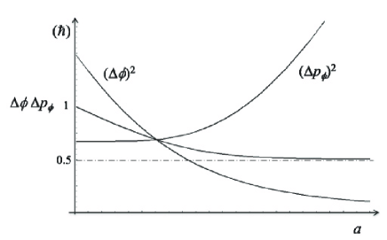
Figure 1: $(\Delta\phi)^{2}$, $(\Delta p_{\phi})^{2}$ and $\Delta\phi\Delta p_{\phi}$, for a value $w=-1$ (vacuum dominated universes).

Now, coherent states for the quantum multiverse can be easily found in the usual way. For the system described by the Hamiltonian (29), the coherent states, $|\alpha,a\rangle$ read Pedrosa87

$$|\alpha,a\rangle=e^{-\frac{|\alpha|^{2}}{2}}\sum_{N=0}^{\infty}\frac{\alpha^{N}}{\sqrt{N!}}e^{i\alpha_{N}(a)}|N,a\rangle,$$ (50)

where, $|N,a\rangle$ and $\alpha_{N}(a)$ are given by Eqs. (36) and (38), respectively. They are the eigenstates of the annihilation operator, $b(a)$, i.e.,

$$b(a)|\alpha,a\rangle=\alpha(a)|\alpha,a\rangle,$$ (51)

where, $\alpha(a)=e^{2i\alpha_{0}(a)}$. The scale-factor dependent annihilation and creation operators are then given by,

$$b(a) = \mu(a)b_{0}+\nu(a)b_{0}^{\dagger},$$ (52)

$$b^{\dagger}(a) = \mu^{*}(a)b_{0}^{\dagger}+\nu^{*}(a)b_{0},$$ (53)

where $b_{0}$ and $b_{0}^{\dagger}$ are the annihilation and creation operators of constant mass and frequency ( say, $m=\omega_{0}=1$), and Pedrosa87

$$\mu(a) = \frac{1}{2}\left(\frac{1}{\rho(a)}+\rho(a)-i\dot{\rho}(a)\right),$$ (54)

$$\nu(a) = \frac{1}{2}\left(\frac{1}{\rho(a)}-\rho(a)-i\dot{\rho}(a)\right),$$ (55)

with, $|\mu|^{2}-|\nu|^{2}=1$. It follows that coherent states in the multiverse turn out to actually be describable as squeezed states Walls83 . The uncertainty in the wavefunction of a single universe and its conjugated momentum are in fact given by,

$$(\Delta\phi)^{2} = \frac{\hbar}{2\omega_{0}}|\mu-\nu|^{2},$$ (56)

$$(\Delta p_{\phi})^{2} = \frac{\hbar\omega_{0}}{2}|\mu+\nu|^{2}.$$ (57)

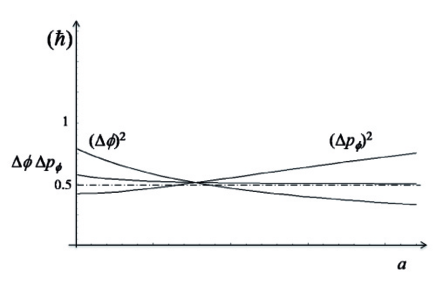
Figure 2: $(\Delta\phi)^{2}$, $(\Delta p_{\phi})^{2}$ and $\Delta\phi\Delta p_{\phi}$, for a value $w=0$ (matter dominated universes).

The evolution of such uncertainties are depicted in Figs. 1 - 3 for different values of the parameter $w$. The squeezing effect becomes larger as the value of $w$ goes away from $\frac{1}{3}$ (i.e., from a radiation dominated universe), at which point the squeezing effect disappears, i.e., $(\Delta\phi)^{2}=(\Delta p_{\phi})^{2}=\Delta\phi\Delta p_{\phi}=\frac{1}{2}$. Therefore, the squeezing effect becomes quite more apparent as one is entering in the accelerated regime of the universe.

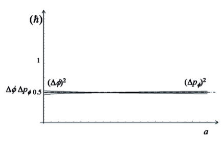
Figure 3: $(\Delta\phi)^{2}$, $(\Delta p_{\phi})^{2}$ and $\Delta\phi\Delta p_{\phi}$, for a value $w=0.3$ (radiation dominated universes; for a value, $w=\frac{1}{3}$, then, $(\Delta\phi)^{2}=(\Delta p_{\phi})^{2}=\Delta\phi\Delta p_{\phi}=\frac{1}{2}$, and no squeezing effect is present).

IV Conclusions and further comments

We have obtained a set of Klauder coherent states for a dark energy dominated universe. They satisfy the boundary conditions and can lead to valid semiclassical approximations. Coherent states represent then a continuous set of states ascribable to the more classical of probable quantum universes, which are in this way interpretable as a multiverse. The different universes residing in such a multiverse differ from one another in a smooth way by the value taken on by the parameter $z$.

Furthermore, in a quantum multiverse scenario in which topological changes are allowed to occur, a third-quantization program has been applied. The state of the multiverse is then obtained in terms of the eigenstates of an harmonic oscillator with mass and frequency which depend on the scale factor. The state of the multiverse is invariant under the energy-matter content of the universes which form up the whole set, and it is also invariant under time reparametrizations, as it should be expected.

In the third-quantized description of the multiverse, coherent states turn out to be converted into squeezed states, the squeezing effect being larger for accelerated universes. Squeezed states entail deeper quantum features which have no classical analogs in the sense that Reid86 they are described by non-classical distributions and can violate the Bell’s inequalities, being related therefore with the highly non-local features of the quantum theory. However, in the context of the quantum multiverse in which the concept of locality and non-locality can no longer be applied, these quantum features would rather be related with the whole universal (independence or non-independence(?)) mutual interrelation of the quantum states of single universes. Therefore, it might well be that accelerated universes, which are described in the third quantization formalism by squeezed states, could not be considered as isolated systems but as really mutually correlated ones within the whole context of the multiverse, whether or not their quantum states had valid classical approximations in the semiclassical regime where $\hbar\rightarrow 0$.

- (1) R. J. Glauber, Phys. Rev. 130, (1963) 2529; R. J. Glauber, Phys. Rev. 131, (1963) 2766.
- (2) J. R. Klauder, J. Math. Phys. 4 (1963) 1058; C. Quesne, J. Phys. A 35 (2002) 9213.
- (3) J. B. Hartle & S. W. Hawking, Phys. Rev. D 28 (1983) 2960.
- (4) D. N. Page, Phys. Rev. D 34 (1986) 2267.
- (5) S. W. Hawking, Phys. Lett. B 195 (1987) 337; S. W. Hawking, Phys. Rev. D 37 (1988) 904; G. V. Lavrelashvili, V. A. Rubakov and P. G. Tinyakov, JETP Lett. 46 (1987) 167; G. V. Lavrelashvili, V. A. Rubakov and P. G. Tinyakov, Nucl. Phys. B 299 (1988) 757.
- (6) A. Strominger, Baby universes, in Quantum Cosmology and Baby Universes, Vol. 7, ed. by S. Coleman, J. B. Hartle, T. Piran and S. Weinberg, World Scientific, London (1990).
- (7) P. F. González-Díaz and S. Robles-Pérez, Int. J. Mod. Phys. D 17 (2008) 1213.
- (8) S. Robles-Pérez, Y. Hassouni and P. F. González-Díaz, Coherent states in quantum cosmology, in Proceedings of the 1st National Meeting on Theoretical Physics, Fes (Morocco), 2007 [arXiv:0709.3302].
- (9) J. B. Hartle, The quantum mechanics of cosmology, in Quantum Cosmology and Baby Universes, Vol. 7, ed. by S. Coleman, J. B. Hartle, T. Piran and S. Weinberg, World Scientific, London (1990).
- (10) Y. Hassouni, E. M. F. Curado and M. A. Rego-Monteiro, Phys. Rev. A 71 (2005) 022104.
- (11) E. M. F. Curado and M. A. Rego-Monteiro, J. Phys. A 34 (2001) 3253.
- (12) A. Vilenkin, Phys. Rev. D 33 (1986) 3560.
- (13) H.R. Lewis and Jr. and W.B. Riesenfeld, J. Math. Phys. 10, 1458 (1969); C. M. A. Dantas, I. A. Pedrosa, and B. Baseia, Phys. Rev. A 45 (1992) 1320; D. Sheng et al., Int. J. Theor. Phys. 34 (1995) 355; D. Song, Phys. Rev. A 62 (2000) 014103.
- (14) I. A. Pedrosa, Phys. Rev. D 36 (1987) 1279; A. D. Jannussis and B. S. Bartzis, Phys. Lett. A 129 (1988) 264.
- (15) D. Walls, Nature 306 (1983) 141.
- (16) M. D. Reid and D. Walls, Phys. Rev. A 34 (1986) 1260.