Technical Report # KU-EC-09-6:
Spatial Clustering Tests Based on Domination Number of a New Random Digraph Family

Abstract

We use the domination number of a parametrized random digraph family called proportional-edge proximity catch digraphs (PCDs) for testing multivariate spatial point patterns. This digraph family is based on relative positions of data points from various classes. We extend the results on the distribution of the domination number of proportional-edge PCDs, and use the domination number as a statistic for testing segregation and association against complete spatial randomness. We demonstrate that the domination number of the PCD has binomial distribution when size of one class is fixed while the size of the other (whose points constitute the vertices of the digraph) tends to infinity and asymptotic normality when sizes of both classes tend to infinity. We evaluate the finite sample performance of the test by Monte Carlo simulations, prove the consistency of the test under the alternatives, and suggest corrections for the support restriction on the class of points of interest and for small samples. We find the optimal parameters for testing each of the segregation and association alternatives. Furthermore, the methodology discussed in this article is valid for data in higher dimensions also.

Keywords: association; complete spatial randomness; consistency; Delaunay triangulation; proximity catch digraph; proximity map; segregation

1 Introduction

In statistical literature, the problem of clustering received considerable attention. The spatial interaction between two or more classes has important implications especially for plant species. See, e.g., Pielou, (1961), Dixon, (1994); Dixon, 2002a , Stoyan and Penttinen, (2000), and Perry et al., (2006). Recently, a new clustering test based on the relative allocation of points from two or more classes has been developed. The method is based on a graph-theoretic approach and is used to test the spatial pattern of complete spatial randomness (CSR) against segregation or association. Rather than the pattern of points from one-class with respect to the ground, the patterns of points from one class with respect to points from other classes are investigated. CSR is roughly defined as the lack of spatial interaction between the points in a given study area. Segregation is the pattern in which points of one class tend to cluster together, i.e., form one-class clumps. On the other hand, association is the pattern in which the points of one class tend to occur more frequently around points from the other class. For convenience and generality, we call the different types of points as “classes”, but the class can be replaced by any characteristic of an observation at a particular location. For example, the pattern of spatial segregation has been investigated for species (Diggle, (2003)), age classes of plants (Hamill and Wright, (1986)) and sexes of dioecious plants (Nanami et al., (1999)).

Many methods to analyze spatial clustering have been proposed in the literature (Kulldorff, (2006)). These include Ripley’s $K$ or $L$-functions (Ripley, (2004)), comparison of NN distances (Diggle, (2003), Cuzick and Edwards, (1990)), and analysis of nearest neighbor contingency tables (NNCTs) which are constructed using the NN frequencies of classes (Pielou, (1961) and Dixon, (1994); Dixon, 2002a ). The tests (i.e., inference) based on Ripley’s $K$ or $L$-functions are only appropriate when the null pattern can be assumed to be the CSR independence pattern, but not if the null pattern is the RL of points from an inhomogeneous Poisson pattern (Kulldorff, (2006)). But, there are also variants of $K(t)$ that explicitly correct for inhomogeneity (see Baddeley et al., (2000)). Cuzick and Edward’s $k$-NN tests are designed for testing bivariate spatial interaction and mostly used for spatial clustering of cases or controls in epidemiology. Diggle’s $D$-function is a modified version of Ripley’s $K$-function (Diggle, (2003)) and is appropriate for the case in which the null pattern is the RL of points where the points are a realization from any arbitrary point pattern. Ripley’s and Diggle’s functions are designed to analyze univariate or bivariate spatial interaction at various scales (i.e., inter-point distances).

In recent years, the use of mathematical graphs has also gained popularity in spatial analysis (Roberts et al., (2000)) providing a way to move beyond Euclidean metrics for spatial analysis. Although only recently introduced to landscape ecology, graph theory is well suited to ecological applications concerned with connectivity or movement (Minor and Urban, (2007)). Conventional graphs do not explicitly maintain geographic reference, reducing utility of other geo-spatial information. Fall et al., (2007) introduce spatial graphs that integrate a geometric reference system that ties patches and paths to specific spatial locations and spatial dimensions thereby preserving the relevant spatial information. However, after a graph is constructed using spatial data, usually the scale is lost (see for instance, Su et al., (2007)). Many concepts in spatial ecology depend on the idea of spatial adjacency which requires information on the close vicinity of an object. Graph theory conveniently can be used to express and communicate adjacency information allowing one to compute meaningful quantities related to spatial point pattern. Adding vertex and edge properties to graphs extends the problem domain to network modeling (Keitt, (2007)). Wu and Murray, (2008) propose a new measure based on graph theory and spatial interaction, which reflects intra-patch and inter-patch relationships by quantifying contiguity within patches and potential contiguity among patches. Friedman and Rafsky, (1983) also propose a graph-theoretic method to measure multivariate association, but their method is not designed to analyze spatial interaction between two or more classes; instead it is an extension of generalized correlation coefficient (such as Spearman’s $\rho$ or Kendall’s $\tau$) to measure multivariate (possibly nonlinear) correlation.

The graph-theoretic method we use to test spatial randomness is based on proximity catch digraphs (PCDs) which are a special type of proximity graphs introduced by Toussaint, (1980). A digraph is a directed graph with vertices $V$ and arcs (directed edges) each of which is from one vertex to another based on a binary relation. Then the pair $(p,q)\in V\times V$ is an ordered pair which stands for an arc from vertex $p$ to vertex $q$ in $V$. For example, nearest neighbor (di)graph which is defined by placing an arc between each vertex and its nearest neighbor is a proximity digraph (Paterson and Yao, (1992)). The nearest neighbor digraph has the vertex set $V$ and $(p,q)$ as an arc iff $q$ is a nearest neighbor of $p$. The domination number of PCDs is first investigated for data in one Delaunay triangle (in $\mathbb{R}^{2}$) and the analysis is generalized to data in multiple Delaunay triangles. Some trivial proofs are omitted and shorter proofs are given in the main body of the article. Data-random digraphs are directed graphs in which each vertex corresponds to a data point, and arcs are defined in terms of some bivariate function on the data. Priebe et al., (2001) introduced a data random digraph called class cover catch digraph (CCCD) in $\mathbb{R}$ and extended it to multiple dimensions. In this model, the vertices correspond to data points from a single class $\mathcal{X}$ and the definition of the arcs utilizes the other class $\mathcal{Y}$. For each $x_{i}\in\mathcal{X}$ a radius is defined as $r_{i}=\min_{\mathsf{y}\in\mathcal{Y}}d(x_{i},\mathsf{y})$. There is an arc from $x_{i}$ to $x_{j}$ if $d(x_{i},x_{j})<r_{i}$; that is, the (open) sphere of radius $r_{i}$ “catches” $x_{j}$. DeVinney et al., (2002), Marchette and Priebe, (2003), Priebe et al., 2003a , and Priebe et al., 2003b demonstrated relatively good performance of CCCDs in classification. Their methods involve data reduction (condensing) by using approximate minimum dominating sets as prototype sets (since finding the exact minimum dominating set is an NP-hard problem in general — e.g., for CCCD in multiple dimensions — (see DeVinney and Priebe, (2006)). For the domination number of CCCDs for one-dimensional data, a SLLN result is proved in (DeVinney and Wierman, (2003)), and this result is extended by Wierman and Xiang, (2008); furthermore, a CLT is also proved by Xiang and Wierman, (2009). The asymptotic distribution of the domination number of CCCDs for non-uniform data in $\mathbb{R}$ is also calculated in a rather general setting (Ceyhan, (2008)). Although intuitively appealing and easy to extend to higher dimensions, finding the minimum dominating set of CCCD is an NP-hard problem and the distribution of the domination number of CCCDs is not analytically tractable for $d>1$. This drawback has motivated us to define new types of proximity maps. As alternatives to CCCD, Ceyhan and Priebe, (2003) introduced an (unparametrized) type of PCDs called central similarity PCDs; Ceyhan and Priebe, (2005) also introduced another parametrized family of PCDs called proportional-edge PCDs and used the domination number of this PCD with a fixed parameter for testing spatial patterns. The domination number approach is appropriate when at least one of the classes is sufficiently large. The relative (arc) density of these PCDs are also used for testing the spatial patterns in (Ceyhan et al., (2006)) and (Ceyhan et al., (2007)). These new PCDs are designed to have better distributional and mathematical properties. These new families are both applicable to pattern classification also. Ceyhan and Priebe, (2003) introduced the central similarity proximity maps and the associated PCDs, and Ceyhan et al., (2007) computed the asymptotic distribution of the relative (arc) density of the parametrized version of the central similarity PCDs and applied the method to testing spatial patterns. Ceyhan and Priebe, (2005) introduced proportional-edge PCD with expansion parameter $r$, where the distribution of the domination number of proportional-edge PCD with $r=3/2$ is used in testing spatial patterns of segregation or association. Ceyhan et al., (2006) computed the asymptotic distribution of the relative density of the proportional-edge PCD and used it for the same purpose. Ceyhan and Priebe, (2007) derived the asymptotic distribution of the domination number of proportional-edge PCDs for uniform data. An extensive treatment of the PCDs based on Delaunay tessellations is available in Ceyhan, (2005).

In this article, we investigate the use of the domination number of proportional-edge PCDs, whose asymptotic distribution was computed in (Ceyhan and Priebe, (2007)) for testing spatial patterns of segregation and association. Furthermore, we extend this result for the whole range of the expansion parameter in a more general setting. By construction, in our PCDs, the further an $\mathcal{X}$ point is from $\mathcal{Y}$ points, it will be more likely to have more arcs to other $\mathcal{X}$ points, hence the domination number will be more likely to be smaller. This probabilistic behavior lends the domination number as a statistic for testing spatial segregation or association. In addition to the mathematical tractability and applicability to testing spatial patterns and classification, this new family of PCDs is more flexible as it allows choosing an optimal parameter for testing against various types of spatial point patterns.

We define proximity maps and the associated PCDs in Section 2, present the asymptotic distribution of the domination number for uniform data in one triangle and in multiple triangles in Section 3, describe the alternative patterns of segregation and association in Section 4, present the Monte Carlo simulation analysis to assess the empirical size and power performance in Section 5, suggest an adjustment for data points from the class of interest which are outside the convex hull of data from the other class in Section 6, suggest a correction method for small sample sizes of the class of interest in Section 7, provide an example data set in Section LABEL:sec:example, and describe the extension of proportional-edge PCDs to higher dimensions in Section 8. We also provide the guidelines in using this test in Section 9.

2 Proximity Maps and the Associated PCDs

Our PCDs are based on the proximity maps which are defined in a fairly general setting. Let $(\Omega,\mathcal{M})$ be a measurable space. The proximity map $N(\cdot)$ is defined as $N:\Omega\rightarrow 2^{\Omega}$, where $2^{\Omega}$ is the power set of $\Omega$. The proximity region associated with $x\in\Omega$, denoted $N(x)$, is the image of $x\in\Omega$ under $N(\cdot)$. The points in $N(x)$ are thought of as being “closer” to $x\in\Omega$ than are the points in $\Omega\setminus N(x)$. Hence the term “proximity” in the name proximity catch digraph. The $\Gamma_{1}$-region $\Gamma_{1}(\cdot)=\Gamma_{1}(\cdot,\mathcal{Y}):\Omega\rightarrow 2^{\Omega}$ associates the region $\Gamma_{1}(x):=\{z\in\Omega:x\in N_{\mathcal{Y}}(z)\}$ with each point $x\in\Omega$. Proximity maps are the building blocks of the proximity graphs of Toussaint, (1980); an extensive survey on proximity maps and graphs is available in (Jaromczyk and Toussaint, (1992)).

The proximity catch digraph $D$ has the vertex set $\mathcal{V}=\bigl{\{}p_{1},\ldots,p_{n}\bigr{\}}$; and the arc set $\mathcal{A}$ is defined by $(p_{i},p_{j})\in\mathcal{A}$ iff $p_{j}\in N(p_{i})$ for $i\not=j$. Notice that the proximity catch digraph $D$ depends on the proximity map $N(\cdot)$ and if $p_{j}\in N(p_{i})$, then we call the region $N(p_{i})$ (and the point $p_{i}$) catches point $p_{j}$. Hence the term “catch” in the name proximity catch digraph. If arcs of the form $(p_{i},p_{i})$ (i.e., loops) were allowed, $D$ would have been called a pseudodigraph according to some authors (see, e.g., Chartrand and Lesniak, (1996)).

In a digraph $D=(\mathcal{V},\mathcal{A})$, a vertex $v\in\mathcal{V}$ dominates itself and all vertices of the form $\{u:(v,u)\in\mathcal{A}\}$. A dominating set $S_{D}$ for the digraph $D$ is a subset of $\mathcal{V}$ such that each vertex $v\in\mathcal{V}$ is dominated by a vertex in $S_{D}$. A minimum dominating set $S^{*}_{D}$ is a dominating set of minimum cardinality and the domination number $\gamma(D)$ is defined as $\gamma(D):=|S^{*}_{D}|$ (see, e.g., Lee, (1998)) where $|\cdot|$ denotes the set cardinality functional. See Chartrand and Lesniak, (1996) and West, (2001) for more on graphs and digraphs. If a minimum dominating set is of size one, we call it a dominating point. Note that for $|\mathcal{V}|=n>0$, $1\leq\gamma(D)\leq n$, since $\mathcal{V}$ itself is always a dominating set.

We construct the proximity regions using two data sets $\mathcal{X}_{n}$ and $\mathcal{Y}_{m}$ of sizes $n$ and $m$ from classes $\mathcal{X}$ and $\mathcal{Y}$, respectively. Given $\mathcal{Y}_{m}\subseteq\Omega$, the proximity map $N_{\mathcal{Y}}(\cdot):\Omega\rightarrow 2^{\Omega}$ associates a proximity region $N_{\mathcal{Y}}(x)\subseteq\Omega$ with each point $x\in\Omega$. The region $N_{\mathcal{Y}}(x)$ is defined in terms of the distance between $x$ and $\mathcal{Y}_{m}$. More specifically, our proportional-edge proximity maps will be based on the relative position of points from $\mathcal{X}_{n}$ with respect to the Delaunay tessellation of $\mathcal{Y}_{m}$. In this article, a triangle refers to the closed region bounded by its edges. See Figure 1 for an example with $n=200$ $\mathcal{X}$ points iid $\mathcal{U}\bigl{(}(0,1)\times(0,1)\bigr{)}$, the uniform distribution on the unit square and the Delaunay triangulation (which yields 13 triangles) is based on $m=10$ $\mathcal{Y}$ points which are also iid $\mathcal{U}\bigl{(}(0,1)\times(0,1)\bigr{)}$ and 77 of these $\mathcal{X}$ points are inside the convex hull of $\mathcal{Y}$ points.

Figure 1: In left, plotted is a realization of $200$ $\mathcal{X}$ points (pluses, $+$) and the Delaunay triangulation based on 10 $\mathcal{Y}$ points (circles, $\circ$). In right, plotted is the 77 $\mathcal{X}$ points which are in the convex hull of $\mathcal{Y}$ points. Both $\mathcal{X}_{n}$ and $\mathcal{Y}_{m}$ are random samples from $\mathcal{U}\bigl{(}(0,1)\times(0,1)\bigr{)}$, the uniform distribution on the unit square.

If $\mathcal{X}_{n}=\bigl{\{}X_{1},\ldots,X_{n}\bigr{\}}$ is a set of $\Omega$-valued random variables then $N_{\mathcal{Y}}(X_{i})$ and $\Gamma_{1}(X_{i})$ are random sets. If $X_{i}$ are iid then so are the random sets $N_{\mathcal{Y}}(X_{i})$. The same holds for $\Gamma_{1}(X_{i})$. We define the data-random proximity catch digraph $D$ — associated with $N_{\mathcal{Y}}(\cdot)$ — with vertex set $\mathcal{X}_{n}=\{X_{1},\cdots,X_{n}\}$ and arc set $\mathcal{A}$ by

$$(X_{i},X_{j})\in\mathcal{A}\iff X_{j}\in N_{\mathcal{Y}}(X_{i}).$$

Since this relationship is not symmetric, a digraph is used rather than a graph. The random digraph $D$ depends on the (joint) distribution of $X_{i}$ and on the map $N_{\mathcal{Y}}(\cdot)$. For $\mathcal{X}_{n}=\bigl{\{}X_{1},\cdots,X_{n}\bigr{\}}$, a set of iid random variables from $F$, the domination number of the associated data-random PCD based on the proximity map $N(\cdot)$, denoted $\gamma(\mathcal{X}_{n},N)$, is the minimum number of point(s) that dominate all points in $\mathcal{X}_{n}$. The random variable $\gamma(\mathcal{X}_{n},N)$ depends explicitly on $\mathcal{X}_{n}$ and $N(\cdot)$ and implicitly on $F$. Furthermore, in general, the distribution, hence the expectation $\mathbf{E}\,[\gamma(\mathcal{X}_{n},N)]$, depends on $n$, $F$, and $N$; $1\leq\mathbf{E}\,[\gamma(\mathcal{X}_{n},N)]\leq n.$ In general, the variance of $\gamma(\mathcal{X}_{n},N)$ satisfies, $1\leq\mathbf{Var}\,[\gamma(\mathcal{X}_{n},N)]\leq n^{2}/4$. For example, the CCCD of Priebe et al., (2001) can be viewed as an example of PCDs and is briefly discussed in the next section. We use some of the properties of CCCD in $\mathbb{R}$ as guidelines in defining PCDs in higher dimensions.

2.1 Spherical Proximity Maps

Priebe et al., (2001) introduced the class cover catch digraphs (CCCDs) and gave the exact and the asymptotic distribution of the domination number of the CCCD based on two sets, $\mathcal{X}_{n}$ and $\mathcal{Y}_{m}$, which are of sizes $n$ and $m$, from classes, $\mathcal{X}$ and $\mathcal{Y}$, respectively, and are sets of iid random variables from uniform distribution on a compact interval in $\mathbb{R}$.

Let $\mathcal{Y}_{m}=\left\{\mathsf{y}_{1},\ldots,\mathsf{y}_{m}\right\}\subset\mathbb{R}$. Then the proximity map associated with CCCD is defined as the open ball $N_{S}(x):=B(x,r(x))$ for all $x\in\mathbb{R}$, where $r(x):=\min_{\mathsf{y}\in\mathcal{Y}_{m}}d(x,\mathsf{y})$ with $d(x,y)$ being the Euclidean distance between $x$ and $y$ (Priebe et al., (2001)). That is, there is an arc from $X_{i}$ to $X_{j}$ iff there exists an open ball centered at $X_{i}$ which is “pure” (or contains no elements) of $\mathcal{Y}_{m}$ in its interior, and simultaneously contains (or “catches”) point $X_{j}$. We consider the closed ball, $\overline{B}(x,r(x))$ for $N_{S}(x)$ in this article. Then for $x\in\mathcal{Y}_{m}$, we have $N_{S}(x)=\{x\}$. Notice that a ball is a sphere in higher dimensions, hence the notation $N_{S}$. Furthermore, dependence on $\mathcal{Y}_{m}$ is through $r(x)$.

A natural extension of the proximity region $N_{S}(x)$ to $\mathbb{R}^{d}$ with $d>1$ is obtained as $N_{S}(x):=B(x,r(x))$ where $r(x):=\min_{\mathsf{y}\in\mathcal{Y}_{m}}d(x,\mathsf{y})$ which is called the spherical proximity map. The spherical proximity map $N_{S}(x)$ is well-defined for all $x\in\mathbb{R}^{d}$ provided that $\mathcal{Y}_{m}\not=\emptyset$. Extensions to $\mathbb{R}^{2}$ and higher dimensions with the spherical proximity map — with applications in classification — are investigated by DeVinney et al., (2002), Marchette and Priebe, (2003), Priebe et al., 2003a ; Priebe et al., 2003b , and DeVinney and Priebe, (2006).

2.2 The Proportional-Edge Proximity Maps

First, we describe the construction of the $r$-factor proximity maps and regions, then state some of its basic properties and introduce some auxiliary tools. Note that in $\mathbb{R}$ the CCCDs are based on the intervals whose end points are from class $\mathcal{Y}$. $I_{i}=\left(\mathsf{y}_{(i-1):m},\mathsf{y}_{i:m}\right)$ for $i=0,\ldots,(m+1)$ with $\mathsf{y}_{0:m}=-\infty$ and $\mathsf{y}_{(m+1):m}=\infty$, where $\mathsf{y}_{i:m}$ is the $i^{th}$ order statistic in $\mathcal{Y}_{m}$. This interval partitioning can be viewed as the Delaunay tessellation of $\mathbb{R}$ based on $\mathcal{Y}_{m}$. So in higher dimensions, we use the Delaunay triangulation based on $\mathcal{Y}_{m}$ to partition the support.

Let $\mathcal{Y}_{m}=\left\{\mathsf{y}_{1},\ldots,\mathsf{y}_{m}\right\}$ be $m$ points in general position in $\mathbb{R}^{d}$ and $T_{i}$ be the $i^{th}$ Delaunay cell for $i=1,\ldots,J_{m}$, where $J_{m}$ is the number of Delaunay cells. Let $\mathcal{X}_{n}$ be a set of iid random variables from distribution $F$ in $\mathbb{R}^{d}$ with support $\mathcal{S}(F)\subseteq\mathcal{C}_{H}(\mathcal{Y}_{m})$ where $\mathcal{C}_{H}(\mathcal{Y}_{m})$ stands for the convex hull of $\mathcal{Y}_{m}$. In particular, for illustrative purposes, we focus on $\mathbb{R}^{2}$ where a Delaunay tessellation is a triangulation, provided that no more than three points in $\mathcal{Y}_{m}$ are cocircular (i.e., lie on the same circle). Furthermore, for simplicity, let $\mathcal{Y}_{3}=\{\mathsf{y}_{1},\mathsf{y}_{2},\mathsf{y}_{3}\}$ be three non-collinear points in $\mathbb{R}^{2}$ and $T(\mathcal{Y}_{3})=T(\mathsf{y}_{1},\mathsf{y}_{2},\mathsf{y}_{3})$ be the triangle with vertices $\mathcal{Y}_{3}$. Let $\mathcal{X}_{n}$ be a set of iid random variables from $F$ with support $\mathcal{S}(F)\subseteq T(\mathcal{Y}_{3})$. If $F=\mathcal{U}(T(\mathcal{Y}_{3}))$, a composition of translation, rotation, reflections, and scaling will take any given triangle $T(\mathcal{Y}_{3})$ to the basic triangle $T_{b}=T((0,0),(1,0),(c_{1},c_{2}))$ with $0<c_{1}\leq 1/2$, $c_{2}>0$, and $(1-c_{1})^{2}+c_{2}^{2}\leq 1$, preserving uniformity. That is, if $X\sim\mathcal{U}(T(\mathcal{Y}_{3}))$ is transformed in the same manner to, say $X^{\prime}$, then we have $X^{\prime}\sim\mathcal{U}(T_{b})$. In fact this will hold for any distribution $F$ up to scale.

For $r\in[1,\infty]$, define $N_{PE}^{r}(\cdot,M):=N(\cdot,M;r,\mathcal{Y}_{3})$ to be the (parametrized) proportional-edge proximity map with $M$-vertex regions as follows (see also Figure 2 with $M=M_{C}$ and $r=2$). For $x\in T(\mathcal{Y}_{3})\setminus\mathcal{Y}_{3}$, let $v(x)\in\mathcal{Y}_{3}$ be the vertex whose region contains $x$; i.e., $x\in R_{M}(v(x))$. In this article $M$-vertex regions are constructed by the lines joining any point $M\in\mathbb{R}^{2}\setminus\mathcal{Y}_{3}$ to a point on each of the edges of $T(\mathcal{Y}_{3})$. Preferably, $M$ is selected to be in the interior of the triangle $T(\mathcal{Y}_{3})^{o}$. For such an $M$, the corresponding vertex regions can be defined using the line segment joining $M$ to $e_{j}$, which lies on the line joining $\mathsf{y}_{j}$ to $M$; e.g., see Figure 3 (left) for vertex regions based on center of mass $M_{C}$, and Figure 3 (right) for vertex regions based on incenter $M_{I}$. With $M_{C}$, the lines joining $M$ and $\mathcal{Y}_{3}$ are the median lines, that cross edges at $M_{j}$ for $j=1,2,3$. $M$-vertex regions, among many possibilities, can also be defined by the orthogonal projections from $M$ to the edges. See Ceyhan, (2005) for a more general definition. The vertex regions in Figure 2 are center of mass vertex regions (i.e., $CM$-vertex regions). If $x$ falls on the boundary of two $M$-vertex regions, we assign $v(x)$ arbitrarily. Let $e(x)$ be the edge of $T(\mathcal{Y}_{3})$ opposite of $v(x)$. Let $\ell(v(x),x)$ be the line parallel to $e(x)$ and passes through $x$. Let $d(v(x),\ell(v(x),x))$ be the Euclidean (perpendicular) distance from $v(x)$ to $\ell(v(x),x)$. For $r\in[1,\infty)$, let $\ell_{r}(v(x),x)$ be the line parallel to $e(x)$ such that

$$d(v(x),\ell_{r}(v(x),x))=r\,d(v(x),\ell(v(x),x))\\ \text{ and }\\ d(\ell(v(x),x),\ell_{r}(v(x),x))<d(v(x),\ell_{r}(v(x),x)).$$

Let $T_{r}(x)$ be the triangle similar to and with the same orientation as $T(\mathcal{Y}_{3})$ having $v(x)$ as a vertex and $\ell_{r}(v(x),x)$ as the opposite edge. Then the proportional-edge proximity region $N_{PE}^{r}(x,M)$ is defined to be $T_{r}(x)\cap T(\mathcal{Y}_{3})$. Notice that $\ell(v(x),x)$ divides the edges of $T_{r}(x)$ (other than the one lies on $\ell_{r}(v(x),x)$) proportionally with the factor $r$. Hence the name proportional-edge proximity region.

Figure 2: Construction of proportional-edge proximity region, $N_{PE}^{r=2}(x,M_{C})$ (shaded region) for an $x$ in the CM-vertex region for $\mathsf{y}_{1}$, $R_{M_{C}}(\mathsf{y}_{1})$.

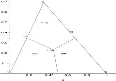
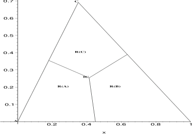
Figure 3: The vertex regions constructed with center of mass $M=M_{C}$ (left) and incenter $M=M_{I}$ (right) using the line segments on the line joining each vertex in $\mathcal{Y}_{3}$ to $M$.

Notice that $r\geq 1$ implies $x\in N_{PE}^{r}(x,M)$ for all $x\in T(\mathcal{Y}_{3})$. Furthermore, $\lim_{r\rightarrow\infty}N_{PE}^{r}(x,M)=T(\mathcal{Y}_{3})$ for all $x\in T(\mathcal{Y}_{3})\setminus\mathcal{Y}_{3}$, so we define $N_{PE}^{\infty}(x,M)=T(\mathcal{Y}_{3})$ for all such $x$. For $x\in\mathcal{Y}_{3}$, we define $N_{PE}^{r}(x,M)=\{x\}$ for all $r\in[1,\infty]$.

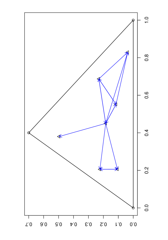
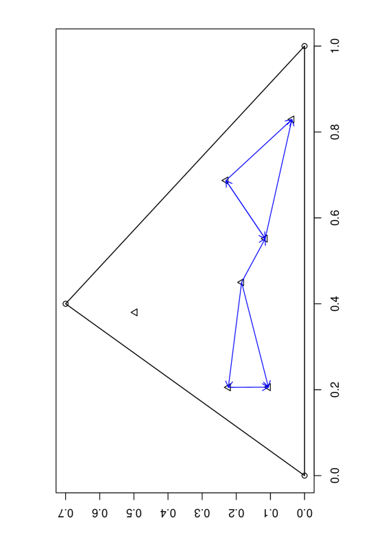
Figure 4: A realization of 7 $\mathcal{X}$ points generated iid $\mathcal{U}(T(\mathcal{Y}_{3}))$, the uniform distribution on $T(\mathcal{Y}_{3})$, (top left) and the corresponding arcs of proportional-edge PCD with $M=M_{C}$ for $r=3/2$ (top right) and $r=5/4$ (bottom).

The proportional-edge PCD has vertices $\mathcal{X}_{n}$ and arcs $(x_{i},x_{j})$ iff $x_{j}\in N_{PE}^{r}(x_{i},M)$. See Figure 4 for a realization of $\mathcal{X}_{n}$ with $n=7$ in one triangle (i.e., $m=3$). For $r=3/2$, the number of arcs is 12 and the domination number $\text{\boldsymbol{\Large$\gamma$}}\left(\mathcal{X}_{n},N_{PE}^{r=3/2}\right)=1$; and for $r=5/4$, the number of arcs is 9 and $\text{\boldsymbol{\Large$\gamma$}}\left(\mathcal{X}_{n},N_{PE}^{r=5/4}\right)=3$. By construction, note that as $x$ gets closer to $M$ (or equivalently further away from the vertices in vertex regions), $N_{PE}^{r}(x,M)$ increases in area, hence it is more likely for the outdegree of $x$ to increase. So if more $\mathcal{X}$ points are around the center $M$, then it is more likely for the domination number $\gamma(\mathcal{X}_{n},N_{PE}^{r})$ to decrease; on the other hand, if more $\mathcal{X}$ points are around the vertices $\mathcal{Y}_{3}$, then the regions get smaller, hence it is more likely for the outdegree for such points to be smaller, thereby implying $\gamma(\mathcal{X}_{n},N_{PE}^{r})$ to increase. We exploit this probabilistic behavior of $\gamma(\mathcal{X}_{n},N_{PE}^{r})$ in testing spatial patterns of segregation and association.

Note also that, $N_{PE}^{r}(x,M)$ can be viewed as a homothetic transformation (enlargement) with $r\geq 1$ applied on a translation of the region $N_{PE}^{r=1}(x,M)$. Furthermore, this transformation is also an affine similarity transformation.

2.3 Some Auxiliary Tools Associated with PCDs

First, notice that $N_{PE}^{r}(x,M)$ is similar to $T(\mathcal{Y}_{3})$ with the similarity ratio being equal to

$$\frac{\min\Bigl{(}d\bigl{(}v(x),\,e(x)\bigr{)},r\,d\bigl{(}v(x),\,\ell(v(x),x)\bigr{)}\Bigr{)}}{d(v(x),\,e(x))}.$$

To define the $\Gamma_{1}$-region, let $\xi_{i}(x)$ be the line such that $\xi_{i}(x)\cap T\left(\mathcal{Y}_{3}\right)\not=\emptyset$ and $r\,d(\mathsf{y}_{i},\xi_{i}(x))=d(\mathsf{y}_{i},\ell(\mathsf{y}_{i},x))$ for $i=1,2,3$. See also Figure 5. Then $\Gamma_{1}^{r}(x,M)=\bigcup_{i=1}^{3}\bigl{(}\Gamma_{1}^{r}(x,M)\cap R_{M}(\mathsf{y}_{i})\bigr{)}$ where $\Gamma_{1}^{r}(x,M)\cap R_{M}(\mathsf{y}_{i})=\{z\in R_{M}(\mathsf{y}_{i}):d(\mathsf{y}_{i},\ell(\mathsf{y}_{i},z))\geq d(\mathsf{y}_{i},\xi_{i}(x)\}$, for $i=1,2,3$. Notice that $r\geq 1$ implies $x\in\Gamma_{1}^{r}(x,M)$. Furthermore, $\lim_{r\rightarrow\infty}\Gamma_{1}^{r}(x,M)=T\left(\mathcal{Y}_{3}\right)$ for all $x\in T\left(\mathcal{Y}_{3}\right)\setminus\mathcal{Y}$, and so we define $\Gamma_{1}^{\infty}(x,M)=T\left(\mathcal{Y}_{3}\right)$ for all such $x$.

For $X_{i}\stackrel{{\scriptstyle iid}}{{\sim}}F$, with the additional assumption that the non-degenerate two-dimensional probability density function $f$ exists with $\operatorname{support}(f)\subseteq T\left(\mathcal{Y}_{3}\right)$, implies that the special case in the construction of $N_{PE}^{r}$ —$X$ falls on the boundary of two vertex regions — occurs with probability zero. Note that for such an $F$, $N_{PE}^{r}(x,M)$ is a triangle a.s. and $\Gamma^{r}_{1}(x,M)$ is a star-shaped (not necessarily convex) polygon.

Figure 5: Construction of the $\Gamma_{1}$-region, $\Gamma_{1}^{2}(x,M_{C})$ (shaded region).

Let $X_{e}:=\operatorname{argmin}_{X\in\mathcal{X}_{n}}d(X,e)$ be the (closest) edge extremum for edge $e$ (i.e., closest point among $\mathcal{X}_{n}$ to edge $e$). Then it is easily seen that $\Gamma^{r}_{1}(\mathcal{X}_{n},M)=\bigcap_{i=1}^{3}\Gamma^{r}_{1}(X_{e_{i}},M)$, where $e_{i}$ is the edge opposite vertex $\mathsf{y}_{i}$, for $i=1,2,3$. So $\Gamma^{r}_{1}(\mathcal{X}_{n},M)\cap R_{M}(\mathsf{y}_{i})=\{z\in R_{M}(\mathsf{y}_{i}):\;d(\mathsf{y}_{i},\ell(\mathsf{y}_{i},z)\geq d(\mathsf{y}_{i},\xi_{i}(X_{e_{i}}))\}$, for $i=1,2,3$.

Let the domination number be $\gamma_{n}(r,F,M):=\gamma_{n}(\mathcal{X}_{n};F,N_{PE}^{r})$ and $X_{[i,1]}:=\operatorname{argmin}_{X\in\mathcal{X}_{n}\cap R_{M}(\mathsf{y}_{i})}d(X,e_{i})$. Then $\gamma_{n}(r,M)\leq 3$ with probability 1, since $\mathcal{X}_{n}\cap R_{M}(\mathsf{y}_{i})\subset N_{PE}^{r}\left(X_{[i,1]},M\right)$ for each of $i=1,2,3$. Thus

$$1\leq\mathbf{E}\,[\gamma_{n}(r,F,M)]\leq 3~{}~{}\text{ and }~{}~{}0\leq\mathbf{Var}\,[\gamma_{n}(r,F,M)]\leq 9/4.$$

In $T(\mathcal{Y}_{3})$, drawing the lines $q_{i}(r,x)$ such that $d(\mathsf{y}_{i},e_{i})=r\,d(\mathsf{y}_{i},q_{i}(r,x))$ for $i\in\{1,2,3\}$ yields another triangle, denoted as $\mathscr{T}_{r}$, for $r<3/2$. See Figure 6 for $\mathscr{T}_{r}$ with $r=\sqrt{2}$.

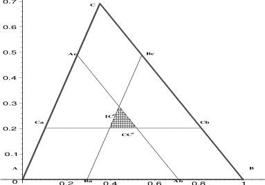
Figure 6: The triangle $\mathscr{T}_{r}$ with $r=\sqrt{2}$ (the hatched region).

The functional form of $\mathscr{T}_{r}$ in the basic triangle $T_{b}$ is given by

$$\mathscr{T}_{r}=T(t_{1}(r),t_{2}(r),t_{3}(r))=\left\{(x,y)\in T_{b}:y\geq\frac{c_{2}\,(r-1)}{r};\;y\leq\frac{c_{2}\,(1-r\,x)}{r\,(1-c_{1})};\;y\leq\frac{c_{2}\,(r\,(x-1)+1)}{r\,c_{1}}\right\}$$ (1)

$$=T\Biggl{(}\left(\frac{(r-1)\,(1+c_{1})}{r},\frac{c_{2}\,(r-1)}{r}\right),\left(\frac{2-r+c_{1}\,(r-1)}{r},\frac{c_{2}\,(r-1)}{r}\right),\left(\frac{c_{1}\,(2-r)+r-1}{r},\frac{c_{2}\,(2-r)}{r}\right)\Biggr{)}.$$

In the standard equilateral triangle, this functional form becomes:

$$\mathscr{T}_{r}=T\Biggl{(}\left(\frac{3\,(r-1)}{2\,r},\frac{\sqrt{3}(r-1)}{2\,r}\right),\left(\frac{3-r}{2\,r},\frac{\sqrt{3}(r-1)}{2\,r}\right),\left(\frac{1}{2},\frac{\sqrt{3}(2-r)}{r}\right)\Biggr{)}.$$

There is a crucial difference between the triangles $\mathscr{T}_{r}$ and $T(M_{1},M_{2},M_{3})$. More specifically $T(M_{1},M_{2},M_{3})\subseteq\mathscr{R}_{S}(r,M)$ for all $M$ and $r\geq 2$, but $(\mathscr{T}_{r})^{o}$ and $\mathscr{R}_{S}(r,M)$ are disjoint for all $M$ and $r$. So if $M\in(\mathscr{T}_{r})^{o}$, then $\mathscr{R}_{S}(r,M)=\emptyset$; if $M\in\partial(\mathscr{T}_{r})$, then $\mathscr{R}_{S}(r,M)=\{M\}$; and if $M\not\in\mathscr{T}_{r}$, then $\mathscr{R}_{S}(r,M)$ has positive area. See Figure 7 for two examples of superset regions with $M$ that corresponds to circumcenter $M_{CC}$ in this triangle and the vertex regions are constructed using orthogonal projections. For $r=2$, note that $\mathscr{T}_{r}=\emptyset$ and the superset region is $T(M_{1},M_{2},M_{3})$ (see Figure 7 (left)), while for $r=\sqrt{2}$, $\mathscr{T}_{r}^{o}$ and $\mathscr{R}_{S}(r=\sqrt{2},M)^{o}$ are disjoint (see Figure 7 (right))

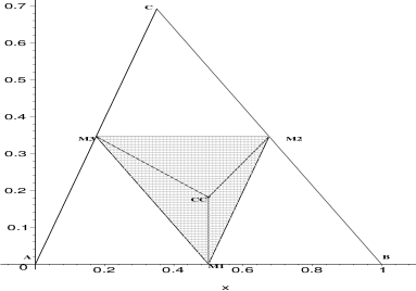
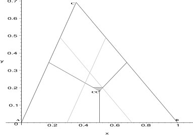
Figure 7: The superset regions (the shaded regions) constructed with circumcenter $M_{CC}$ with $r=\sqrt{2}$ (left) and $r=2$ (right) with vertex regions constructed with orthogonal projections to the edges.

The triangle $\mathscr{T}_{r}$ given in Equation (1) plays an important role in the distribution of the domination number of the proportional-edge PCDs.

3 The Asymptotic Distribution of Domination Number for Uniform Data

3.1 The One-Triangle Case

For simplicity, we consider $\mathcal{X}$ points iid uniform in one triangle only. The null hypothesis we consider is a type of complete spatial randomness; that is,

$$H_{o}:X_{i}\stackrel{{\scriptstyle iid}}{{\sim}}\mathcal{U}(T\left(\mathcal{Y}_{3}\right))\text{ for }i=1,2,\ldots,n,$$

where $\mathcal{U}(T\left(\mathcal{Y}_{3}\right))$ is the uniform distribution on $T\left(\mathcal{Y}_{3}\right)$. If it is desired to have the sample size be a random variable, we may consider a spatial Poisson point process on $T\left(\mathcal{Y}_{3}\right)$ as our null hypothesis. Let $\gamma_{n}(r,M):=\gamma\left(\mathcal{X}_{n},\mathcal{U}(T(\mathcal{Y}_{3})),N_{PE}^{r},M\right)$ be the domination number of the PCD based on $N_{PE}^{r}$ with $\mathcal{X}_{n}$, a set of iid random variables from $\mathcal{U}(T(\mathcal{Y}_{3}))$, with $M$-vertex regions.

We present a “geometry invariance” result for $N_{PE}^{r}(\cdot,M)$ where $M$-vertex regions are constructed using the line segment joining $M$ to edge $e_{i}$ on the line joining $\mathsf{y}_{i}$ to $M$, rather than the orthogonal projections from $M$ to the edges. This invariance property will simplify the notation in our subsequent analysis by allowing us to consider the special case of the (standard) equilateral triangle.

Theorem 3.1.

(Geometry Invariance Property) Suppose $\mathcal{X}_{n}$ is a set of iid random variables from $\mathcal{U}(T(\mathcal{Y}_{3}))$. Then for any $r\in[1,\infty]$ the distribution of $\gamma_{n}(r,M)$ is independent of $\mathcal{Y}_{3}$ and hence the geometry of $T(\mathcal{Y}_{3})$.

Proof: See Ceyhan and Priebe, (2007) for the proof. $\blacksquare$

Note that geometry invariance of $\gamma_{n}(r=\infty,M)$ follows trivially for all $\mathcal{X}_{n}$ from any $F$ with support in $T(\mathcal{Y}_{3})\setminus\mathcal{Y}_{3}$, since for $r=\infty$, we have $\gamma_{n}(r=\infty,M)=1$ a.s. Based on Theorem 3.1 we may assume that $T(\mathcal{Y}_{3})$ is a standard equilateral triangle with $\mathcal{Y}_{3}=\{(0,0),(1,0),\left(1/2,\sqrt{3}/2\right)\}$ for $N_{PE}^{r}(\cdot,M)$ with $M$-vertex regions.

Remark 3.2.

Notice that, we proved the geometry invariance property for $N_{PE}^{r}(\cdot)$ where $M$-vertex regions are defined with the lines joining $\mathcal{Y}_{3}$ to $M$. On the other hand, if we use the orthogonal projections from $M$ to the edges, the vertex regions (hence $N_{PE}^{r}$) will depend on the geometry of the triangle. That is, the orthogonal projections from $M$ to the edges will not be mapped to the orthogonal projections in the standard equilateral triangle. Hence with the orthogonal projections, the exact and asymptotic distribution of $\gamma_{n}(r,M)$ will depend on $c_{1},c_{2}$ of $T_{b}$, so one needs to do the calculations for each possible combination of $c_{1},c_{2}$. $\square$

The domination number $\gamma_{n}(r,M)$ of the PCD has the following asymptotic distribution (Ceyhan and Priebe, (2007)). As $n\rightarrow\infty$,

$$\gamma_{n}(r,M)\stackrel{{\scriptstyle\mathcal{L}}}{{\longrightarrow}}\left\{\begin{array}[]{ll}2+\operatorname{BER}(1-p_{r})&\text{for $r\in[1,3/2)$ and $M\in\{t_{1}(r),t_{2}(r),t_{3}(r)\}$,}\\ 1&\text{for $r>3/2$ and $M\in T(\mathcal{Y}_{3})^{o}$,}\\ 3&\text{for $r\in[1,3/2)$ and $M\in\mathscr{T}_{r}\setminus\{t_{1}(r),t_{2}(r),t_{3}(r)\}$,}\\ \end{array}\right.$$ (2)

where $\stackrel{{\scriptstyle\mathcal{L}}}{{\longrightarrow}}$ stands for “convergence in law” and $\operatorname{BER}(p)$ stands for Bernoulli distribution with probability of success $p$, $\mathscr{T}_{r}$ and $t_{i}(r)$ are defined in Equation (1), and for $r\in[1,3/2)$ and $M\in\{t_{1}(r),t_{2}(r),t_{3}(r)\}$,

$$p_{r}=\int_{0}^{\infty}\int_{0}^{\infty}\frac{64\,r^{2}}{9\,(r-1)^{2}}\,w_{1}\,w_{3}\,\exp\left(\frac{4\,r}{3\,(r-1)}\,(w_{1}^{2}+w_{3}^{2}+2\,r\,(r-1)\,w_{1}\,w_{3})\right)\,dw_{3}w_{1},$$ (3)

and for $r=3/2$ and $M=M_{C}=\left\{(1/2,\sqrt{3}/6)\right\}$, $p_{r}\approx 0.7413$, which is not computed as in Equation (3); for its computation, see Ceyhan and Priebe, (2005). For example, for $r=5/4$ and $M\in\left\{t_{1}(r)=\left(3/10,\sqrt{3}/10\right),t_{2}(r)=\\ \left(7/10,\sqrt{3}/10\right),t_{3}(r)=\left(1/2,3\sqrt{3}/5\right)\right\}$, $p_{r}\approx 0.6514$. See Figure 8 for the plot of the numerically computed values (i.e., the values computed by numerical integration) of $p_{r}$ as a function of $r$ according to Equation (3). Notice that in the nondegenerate case in (2), $\mathbf{E}\,[\gamma_{n}(r,M)]=3-p_{r}$ and $\mathbf{Var}\,[\gamma_{n}(r,M)]=p_{r}(1-p_{r})$.

In Equation (2), the first line is referred as the non-degenerate case, the second and third lines are referred as degenerate cases with a.s. limits 1 and 3, respectively.

Figure 8: Plotted is the probability $p_{r}=\lim_{n\rightarrow\infty}P\left(\gamma_{n}(r,M)=2\right)$ given in Equation (3) as a function of $r$ for $r\in[1,3/2)$ and $M\in\{t_{1}(r),t_{2}(r),t_{3}(r)\}$.

$r=2$ and $M=M_{C}$ $k\diagdown n$ 10 20 30 50 100 1 961 1000 1000 1000 1000 2 34 0 0 0 0 3 5 0 0 0 0

$r=5/4$ and $M=M_{C}$ $k\diagdown n$ 10 20 30 50 100 1 9 0 0 0 0 2 293 110 30 8 0 3 698 890 970 992 1000

Table 1: The number of $\gamma_{n}(r,M)=k$ out of $N=1000$ Monte Carlo replicates with $M=M_{C}$ and $r=2$ (left) and $r=5/4$ (right). Here, “$r=2$ and $M=M_{C}$” is an example of the case “$r>3/2$ and $M\in T(\mathcal{Y}_{3})^{o}$”, and “$r=5/4$ and $M=M_{C}$” is an example of the case “$r\in[1,3/2)$ and $M\in\mathscr{T}_{r}\setminus\{t_{1}(r),t_{2}(r),t_{3}(r)\}$”.

$r=5/4$ and $M=\left(3/5,\sqrt{3}/10\right)$
$k\diagdown n$	10	20	30	50	100	500	1000	2000
1	118	60	51	39	15	1	2	1
2	462	409	361	299	258	100	57	29
3	420	531	588	662	727	899	941	970

$r=5/4$ and $M=\left(7/10,\sqrt{3}/10\right)$
$k\diagdown n$	10	20	30	50	100	500	1000	2000
1	174	118	82	61	22	5	1	1
2	532	526	548	561	611	617	633	649
3	294	356	370	378	367	378	366	350

Table 2: The number of $\gamma_{n}(r,M)=k$ out of $N=1000$ Monte Carlo replicates with $r=5/4$ and $M=\left(3/5,\sqrt{3}/10\right)$ (top) and $M=\left(7/10,\sqrt{3}/10\right)$ (bottom). Here “$r=5/4$ and $M=(3/5,\sqrt{3}/10)$” is an example of the case “$r\in[1,3/2)$ and $M\in\mathscr{T}_{r}\setminus\{t_{1}(r),t_{2}(r),t_{3}(r)\}$” with $M$ being on the line segment joining $t_{1}(r)$ and $t_{2}(r)$, and “$r=5/4$ and $M=(7/10,\sqrt{3}/10)$” is an example of the case “$r\in[1,3/2)$ and $M\in\mathscr{T}_{r}\setminus\{t_{1}(r),t_{2}(r),t_{3}(r)\}$” with $M=t_{2}(r)$.

We also estimate the distribution of $\gamma_{n}(r,M)$ for various values of $n$, $r$, and $M$ using Monte Carlo simulations. At each Monte Carlo replication, we generate $n$ points iid $\mathcal{U}(T(\mathcal{Y}_{3}))$ and compute the value of $\gamma_{n}(r,M)$. The frequencies of $\gamma_{n}(r,M)=k$ out of $N=1000$ Monte Carlo replicates are presented in Tables 1, 2, and 3. Notice that in Table 1 (left) “$r=2$ and $M=M_{C}$” is an example of the case “$r>3/2$ and $M\in T(\mathcal{Y}_{3})^{o}$”, in Table 1 (right) “$r=5/4$ and $M=M_{C}$” is an example of the case “$r\in[1,3/2)$ and $M\in\mathscr{T}_{r}\setminus\{t_{1}(r),t_{2}(r),t_{3}(r)\}$”; in Table 2 (top) “$r=5/4$ and $M=(3/5,\sqrt{3}/10)$” is an example of the case “$r\in[1,3/2)$ and $M\in\mathscr{T}_{r}\setminus\{t_{1}(r),t_{2}(r),t_{3}(r)\}$” with $M$ being on the line segment joining $t_{1}(r)$ and $t_{2}(r)$, in Table 2 (bottom) “$r=5/4$ and $M=(7/10,\sqrt{3}/10)$” is an example of the case “$r\in[1,3/2)$ and $M\in\mathscr{T}_{r}\setminus\{t_{1}(r),t_{2}(r),t_{3}(r)\}$” with $M=t_{2}(r)$; and in Table 3, “$r=3/2$ and $M=M_{C}$” is an example of the case discussed in (Ceyhan and Priebe, (2005)). Notice that as the sample size $n$ increases, the values on these tables get closer and closer to the expected values under their asymptotic distribution.

$r=3/2$ and $M=M_{C}$
$k\diagdown n$	10	20	30	50	100	500	1000	2000
1	151	82	61	50	27	2	3	1
2	602	636	688	693	718	753	729	749
3	247	282	251	257	255	245	268	250

Table 3: The number of $\gamma_{n}(3/2,M_{C})=k$ out of $N=1000$ Monte Carlo replicates. Here “$r=3/2$ and $M=M_{C}$” is an example of the case discussed in (Ceyhan and Priebe, (2005)).

Theorem 3.3.

Let $\gamma_{n}(r,M)=\gamma(\mathcal{X}_{n};\mathcal{U}(T\left(\mathcal{Y}_{3}\right)),N_{PE}^{r},M)$. Then $r_{1}<r_{2}$ implies $\gamma_{n}(r_{2},M)<^{ST}\gamma_{n}(r_{1},M)$ where $<^{ST}$ stands for “stochastically smaller than”.

Proof: Suppose $r_{1}<r_{2}$. Then $P(\gamma_{n}(r_{2},M)=1)>P(\gamma_{n}(r_{1},M)=1)$ and $P(\gamma_{n}(r_{2},M)=2)>P(\gamma_{n}(r_{1},M)=2)$ and $P(\gamma_{n}(r_{2},M)=3)<P(\gamma_{n}(r_{1},M)=3)$. Hence the desired result follows. $\blacksquare$

3.2 The Multi-Triangle Case

In this section, we present the asymptotic distribution of the domination number of proportional-edge PCDs in multiple Delaunay triangles. Suppose $\mathcal{Y}_{m}=\{\mathsf{y}_{1},\mathsf{y}_{2},\ldots,\mathsf{y}_{m}\}\subset\mathbb{R}^{2}$ be a set of $m$ points in general position with $m>3$ and no more than 3 points are cocircular. Then there are $J_{m}>1$ Delaunay triangles each of which is denoted as $T_{j}$ (Okabe et al., (2000)). We wish to investigate

$$H_{o}:X_{i}\stackrel{{\scriptstyle iid}}{{\sim}}\mathcal{U}(C_{H}(\mathcal{Y}_{m}))\text{ for }i=1,2,\ldots,n$$ (4)

against segregation and association alternatives (see Section 4). Figure 13 (middle) presents a realization of 1000 observations independent and identically distributed according to $\mathcal{U}(C_{H}(\mathcal{Y}_{m}))$ for $m=10$ and $J_{m}=13$.

Let $M^{j}$ be the point in $T_{j}$ that corresponds to $M$ in $T_{e}$, $\mathscr{T}_{r}^{j}$ be the triangle that corresponds to $\mathscr{T}_{r}$ in $T_{e}$, and $t_{i}^{j}(r)$ be the vertices of $\mathscr{T}_{r}^{j}$ that correspond to $t_{i}(r)$ in $T_{e}$ for $i\in\{1,2,3\}$. Moreover, let $n_{j}:=|\mathcal{X}_{n}\cap T_{j}|$, the number of $\mathcal{X}$ points in Delaunay triangle $T_{j}$. The digraph $D$ is constructed using $N_{PE}^{r}(\cdot,M^{j})$ as described above, where the three points in $\mathcal{Y}_{m}$ defining the Delaunay triangle $T_{j}$ are used as $\mathcal{Y}_{m(j)}$. Then we have $\geq J_{m}$ disconnected sub-digraphs. For $\mathcal{X}_{n}\subset\mathcal{C}_{H}(\mathcal{Y}_{m})$, let $\gamma_{n_{j}}(r,M^{j})$ be the domination number of the digraph induced by vertices of $T_{j}$ and $\mathcal{X}_{n}\cap T_{j}$. Then the domination number of the proportional-edge PCD in $J_{m}$ triangles is

$$\gamma_{n,m}(r,M)=\sum_{j=1}^{J_{m}}\gamma_{n_{j}}\left(r,M^{j}\right).$$

See Figure 9 for two examples of the proportional edge PCDs based on the 77 $\mathcal{X}$ points that are in $\mathcal{C}_{H}(\mathcal{Y}_{m})$ out of the 200 $\mathcal{X}$ points plotted in Figure 1. The arcs are constructed for $M=M_{C}$ with $r=3/2$ (left) and $r=5/4$ (right) and the corresponding domination number values are $\gamma_{n,10}(3/2,M_{C})=22$ and $\gamma_{n,10}(5/4,M_{C})=26$. Suppose $\mathcal{X}_{n}$ is a set of iid random variables from $\mathcal{U}(\mathcal{C}_{H}(\mathcal{Y}_{m}))$, the uniform distribution on convex hull of $\mathcal{Y}_{m}$ and we construct the proportional-edge PCDs using the points $M^{j}$ that correspond to $M$ in $T_{e}$. Then For fixed $m$ (or fixed $J_{m}$), as $n\rightarrow\infty$, so does each $n_{j}$. Furthermore, as $n\rightarrow\infty$, each component $\gamma_{n_{j}}(r,M^{j})$ become independent. Therefore using Equation (2), we can obtain the asymptotic distribution of $\gamma_{n,m}(r,M)$. For fixed $J_{m}$, as $n\rightarrow\infty$,

$$\gamma_{n,m}(r,M)\stackrel{{\scriptstyle\mathcal{L}}}{{\longrightarrow}}\left\{\begin{array}[]{ll}2\,J_{m}+\operatorname{BIN}(J_{m},1-p_{r})&\text{for $M^{j}\in\left\{t^{j}_{1}(r),t^{j}_{2}(r),t^{j}_{3}(r)\right\}$ and $r\in[1,3/2]$,}\\ J_{m}&\text{for $r>3/2$ and for all $M^{j}\not=\mathcal{Y}_{3}$,}\\ 3\,J_{m}&\text{for $M\in\mathscr{T}_{r}^{j}\setminus\left\{t^{j}_{1}(r),t^{j}_{2}(r),t^{j}_{3}(r)\right\}$ and $r\in[1,3/2)$,}\\ \end{array}\right.$$ (5)

where $\operatorname{BIN}(n,p)$ stands for binomial distribution with $n$ trials and probability of success $p$, for $r\in[1,3/2)$ and $M\in\{t_{1}(r),t_{2}(r),t_{3}(r)\}$, $p_{r}$ is given in Equation (3) and $j=1,2,\ldots,J_{m}$. Observe that in the nondegenerate case in Equation (5), we have $\mathbf{E}\,[\gamma_{n,m}(r,M)]=J_{m}(3-p_{r})$ and $\mathbf{Var}\,[\gamma_{n,m}(r,M)]=J_{m}\,p_{r}\,(1-p_{r})$.

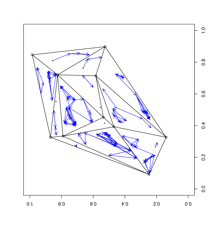
Figure 9: The arcs for the 77 $\mathcal{X}$ points (dots, $\centerdot$) in the convex hull of $\mathcal{Y}$ points (circles, $\circ$) given in Figure 1 for the proportional-edge PCD with $M=M_{C}$ for $r=3/2$ (left) and $r=5/4$ (right).

Theorem 3.4.

(Asymptotic Normality) Suppose $n_{j}$ and $J_{m}$ are sufficiently large with $n_{j}\gg J_{M}$. Then the asymptotic null distribution of the mean domination number (per triangle) $\displaystyle\overline{G}(r,M):=\frac{1}{J_{m}}\,\sum_{j=1}^{J_{m}}\gamma_{n_{j}}(r,M)=\frac{\gamma_{n,m}(r,M)}{J_{m}}$ is approximately normal; i.e., for large $n_{j}\gg J_{M}$

$$\overline{G}(r,M)\stackrel{{\scriptstyle\text{approx}}}{{\Large\sim}}\mathcal{N}(\mu,\sigma^{2}/J_{m})$$

where $\mu=3-p_{r}$ and $\sigma^{2}=p_{r}(1-p_{r})/J_{m}$.

Proof: For fixed $J_{m}$ sufficiently large and each $n_{j}$ sufficiently large with $n=\sum_{j=1}^{J_{m}}n_{j}\gg J_{m}$, $\gamma_{n_{j}}(r,M)$ are approximately independent identically distributed as in Equation (2). Then the desired result follows. $\blacksquare$

In Figure 10 (top), we plot the histograms and the approximating normal curves for $\overline{G}(r,M)$ with $r=3/2$ and $M=M_{C}$ for $n=100,1000$, and 5000 $\mathcal{X}$ points generated iid $\mathcal{U}(C_{H}(\mathcal{Y}_{m}))$ where $\mathcal{Y}_{m}$ (which yields $J_{m}=13$ triangles) is given in Figure 1. Notice that, even though the distribution looks symmetric with $n=100$, the normal approximation is not appropriate, since not all $n_{j}$ are sufficiently large to make the binomial distribution hold as in Equation (5), but as $n$ increases (see $n=1000$ and $n=5000$ cases) the histograms and the corresponding normal curves become more similar indicating that the asymptotic normal approximation gets better, since all $n_{j}$ are sufficiently large. However, larger $J_{m}$ values require larger sample sizes in order to obtain approximate normality. With $J_{20}=30$ triangles based on the Delaunay triangulation of $20$ $\mathcal{Y}$ points iid uniform on the unit square (not presented), we plot the histograms and the approximating normal curves for $r=3/2$ and $M=M_{C}$ in Figure 10 (bottom). Observe that with more triangles (i.e., as $J_{m}$ increases), the normal approximation gets better. We also present the histograms of the mean domination number and the approximating normal curves for $r=5/4$ and $M=(7/10,\sqrt{3}/10)$ in Figure 11, where the trend is similar to the one in Figure 10 (top).

\psfrag{Density}{ \Huge{\bf{Density}}}\includegraphics{normgamma1.ps}

\psfrag{Density}{ \Huge{\bf{Density}}}\includegraphics{normgamma1n1000.ps}

\psfrag{Density}{ \Huge{\bf{Density}}}\includegraphics{normgamma1n5000.ps}

\psfrag{Density}{ \Huge{\bf{Density}}}\includegraphics{normgamma1J30.ps}

\psfrag{Density}{ \Huge{\bf{Density}}}\includegraphics{normgamma1J30n3000.ps}

\psfrag{Density}{ \Huge{\bf{Density}}}\includegraphics{normgamma1J30n5000.ps}

Figure 10: Depicted in the top row are $\overline{G}(r=3/2,M=M_{C})\stackrel{{\scriptstyle\text{approx}}}{{\sim}}\mathcal{N}(\mu\approx 2.2587,\sigma^{2}/J_{10}\approx.1918/J_{10})$ for $J_{10}=13$ and $n=100$ (left), $n=1000$ (middle), and $n=5000$ (right). In the bottom row, depicted are $\overline{G}(r=3/2,M=M_{C})\stackrel{{\scriptstyle\text{approx}}}{{\sim}}\mathcal{N}(\mu\approx 2.2587,\sigma^{2}/J_{20}\approx.1918/J_{20})$ for $J_{20}=30$ and $n=100$ (left), $n=1000$ (middle), and $n=5000$ (right). Histograms are based on $1000$ Monte Carlo replicates and the curves are the associated approximating normal curves.

\psfrag{Density}{ \Huge{\bf{Density}}}\includegraphics{normgamma1J13r54n100.ps}

\psfrag{Density}{ \Huge{\bf{Density}}}\includegraphics{normgamma1J13r54n1000.ps}

\psfrag{Density}{ \Huge{\bf{Density}}}\includegraphics{normgamma1J13r54n5000.ps}

Figure 11: Depicted are $\overline{G}(r=5/4,M=\left(7/10,\sqrt{3}/10\right)\stackrel{{\scriptstyle\text{approx}}}{{\sim}}\mathcal{N}(\mu\approx 2.3486,\sigma^{2}/J_{10}\approx.2271/J_{10})$ for $J_{10}=13$ and $n=100$ (left), $n=1000$ (middle), and $n=5000$ (right). Histograms are based on $1000$ Monte Carlo replicates and the curves are the associated approximating normal curves.

For finite $n$, let $\overline{G}(r,M)$ be the mean domination number (per triangle) associated with the digraph based on $N_{PE}^{r}$. Then as a corollary to Theorem 3.3, it follows that for $r_{1}<r_{2}$, we have $\overline{G}(r_{2},M)<^{ST}\overline{G}(r_{1},M)$.

4 Alternative Patterns: Segregation and Association

In a two class setting, the phenomenon known as segregation occurs when members of one class have a tendency to repel members of the other class. For instance, it may be the case that one type of plant does not grow well in the vicinity of another type of plant, and vice versa. This implies, in our notation, that $X_{i}$ are unlikely to be located near any elements of $\mathcal{Y}$. Alternatively, association occurs when members of one class have a tendency to attract members of the other class, as in symbiotic species, so that the $X_{i}$ will tend to cluster around the elements of $\mathcal{Y}$, for example. See, for instance, Dixon, (1994) and Coomes et al., (1999).

These alternatives can be parametrized as follows: In the one triangle case, without loss of generality let $\mathcal{Y}_{3}=\left\{(0,0),(1,0),(c_{1},c_{2})\right\}$ and $T_{b}=T(\mathcal{Y}_{3})$ with $\mathsf{y}_{1}=(0,0),\mathsf{y}_{2}=(1,0)$, and $\mathsf{y}_{3}=(c_{1},c_{2})$. For the basic triangle $T_{b}$, let $Q_{\theta}:=\{x\in T_{b}:d(x,\mathcal{Y}_{3})\leq\theta\}$ for $\theta\in(0,(c_{1}^{2}+c_{2}^{2})/2]$ and $S(F)$ be the support of $F$. Then consider

$$\mathscr{H}_{S}:=\{F:S(F)\subseteq T_{b}\text{ and }P_{F}(X\in Q_{\theta})<P_{U}(X\in Q_{\theta})\}$$

and

$$\mathscr{H}_{A}:=\{F:S(F)\subseteq T_{b}\text{ and }P_{F}(X\in Q_{\theta})>P_{U}(X\in Q_{\theta})\}$$

where $P_{F}$ and $P_{U}$ are probabilities with respect to distribution function $F$ and the uniform distribution on $T_{b}$, respectively. So if $X_{i}\stackrel{{\scriptstyle iid}}{{\sim}}F\in\mathscr{H}_{S}$, the pattern between $\mathcal{X}$ and $\mathcal{Y}$ points is segregation, but if $X_{i}\stackrel{{\scriptstyle iid}}{{\sim}}F\in\mathscr{H}_{A}$, the pattern between $\mathcal{X}$ and $\mathcal{Y}$ points is association. For example the distribution family

$$\mathscr{F}_{S}:=\{F:S(F)\subset T_{b}\text{ and the associated pdf $f$ increases as $d(x,\mathcal{Y}_{3})$ increases}\}$$

is a subset of $\mathscr{H}_{S}$ and yields samples from the segregation alternatives. Likewise, the distribution family

$$\mathscr{F}_{A}:=\{F:S(F)\subset T_{b}\text{ and the associated pdf $f$ increases as $d(x,\mathcal{Y}_{3})$ decreases}\}$$

is a subset of $\mathscr{H}_{A}$ and yields samples from the association alternatives.

In the basic triangle, $T_{b}$, we define the $H^{S}_{\varepsilon}$ and $H^{A}_{\varepsilon}$ with $\varepsilon\in\left(0,\sqrt{3}/3\right)$, for segregation and association alternatives, respectively. Under $H^{S}_{\varepsilon}$, $4\varepsilon^{2}/3\times 100$ % of the area of $T_{b}$ is chopped off around each vertex so that the $\mathcal{X}$ points are restricted to lie in the remaining region. That is, for $\mathsf{y}_{j}\in\mathcal{Y}_{3}$, let $e_{j}$ denote the edge of $T_{b}$ opposite vertex $\mathsf{y}_{j}$ for $j=1,2,3$, and for $x\in T_{b}$ let $\ell_{j}(x)$ denote the line parallel to $e_{j}$ through $x$. Then define $T_{j}(\varepsilon)=\{x\in T_{b}:d(\mathsf{y}_{j},\ell_{j}(x))\leq\varepsilon_{j}\}$ where $\displaystyle\varepsilon_{1}=\frac{2c_{2}\varepsilon}{3\sqrt{c_{2}^{2}+(1-c_{1})^{2}}}$, $\displaystyle\varepsilon_{2}=\frac{2c_{2}\varepsilon}{3\sqrt{c_{1}^{2}+c_{2}^{2}}}$, and $\displaystyle\varepsilon_{3}=\frac{2c_{2}\varepsilon}{3}$. Let $\mathcal{T}_{\varepsilon}:=\bigcup_{j=1}^{3}T_{j}(\varepsilon)$. Then under $H^{S}_{\varepsilon}$ we have $X_{i}\stackrel{{\scriptstyle iid}}{{\sim}}\mathcal{U}\left(T_{b}\setminus\mathcal{T}_{\varepsilon}\right)$. Similarly under $H^{A}_{\varepsilon}$ we have $X_{i}\stackrel{{\scriptstyle iid}}{{\sim}}\mathcal{U}\left(\mathcal{T}_{\sqrt{3}/3-\varepsilon}\right)$. Thus the segregation model excludes the possibility of any $X_{i}$ occurring around a $\mathsf{y}_{j}$, and the association model requires that all $X_{i}$ occur around $\mathsf{y}_{j}$’s. The $\sqrt{3}/3-\varepsilon$ is used in the definition of the association alternative so that $\varepsilon=0$ yields $H_{o}$ under both classes of alternatives. Thus, we have the below distribution families under this parametrization.

$$\mathscr{U}_{\varepsilon}^{S}:=\{F:F=\mathcal{U}(T_{b}\setminus\mathcal{T}_{\varepsilon})\}\text{ ~{}and~{} }\mathscr{U}_{\varepsilon}^{A}:=\{F:F=\mathcal{U}(\mathcal{T}_{\sqrt{3}/3-\varepsilon})\}.$$ (6)

Clearly $\mathscr{U}_{\varepsilon}^{S}\subsetneq\mathscr{H}_{S}$ and $\mathscr{U}_{\sqrt{3}/3-\varepsilon}^{A}\subsetneq\mathscr{H}_{A}$, but $\mathscr{U}_{\varepsilon}^{S}\nsubseteq\mathscr{F}_{S}$ and $\mathscr{U}_{\sqrt{3}/3-\varepsilon}^{A}\nsubseteq\mathscr{F}_{A}$.

These alternatives $H^{S}_{\varepsilon}$ and $H^{A}_{\varepsilon}$ with $\varepsilon\in\left(0,\sqrt{3}/3\right)$, can be transformed into the equilateral triangle as in (Ceyhan et al., (2006) and Ceyhan et al., (2007)).

For the standard equilateral triangle, in $T_{j}(\varepsilon)=\{x\in T_{e}:d(\mathsf{y},\ell_{j}(x))\leq\varepsilon_{j}\}$ we have $\varepsilon_{1}=\varepsilon_{2}=\varepsilon_{3}=\varepsilon$. Thus $H^{S}_{\varepsilon}$ implies $X_{i}\stackrel{{\scriptstyle iid}}{{\sim}}\mathcal{U}\left(T_{e}\setminus\mathcal{T}_{\varepsilon}\right)$ and $H^{A}_{\varepsilon}$ be the model under which $X_{i}\stackrel{{\scriptstyle iid}}{{\sim}}\mathcal{U}\left(\mathcal{T}_{\sqrt{3}/3-\varepsilon}\right)$. See Figure 12 for a depiction of the above segregation and the association alternatives in $T_{e}$.

Figure 12: An example for the segregation alternative for a particular $\varepsilon$ (shaded region), and its complement is for the association alternative (unshaded region) on the standard equilateral triangle.

Remark 4.1.

These definitions of the alternatives $H^{S}_{\varepsilon}$ and $H^{A}_{\varepsilon}$ are given for the standard equilateral triangle. The geometry invariance result of Theorem 3.1 still holds under the alternatives $H^{S}_{\varepsilon}$ and $H^{A}_{\varepsilon}$. In particular, the segregation alternative with $\varepsilon\in\left(0,\sqrt{3}/4\right)$ in the standard equilateral triangle corresponds to the case that in an arbitrary triangle, $\delta\cdot 100\%$ of the area is carved away as forbidden from the vertices using line segments parallel to the opposite edge where $\delta=4\varepsilon^{2}$ (which implies $\delta\in(0,3/4)$). But the segregation alternative with $\varepsilon\in\left(\sqrt{3}/4,\sqrt{3}/3\right)$ in the standard equilateral triangle corresponds to the case that in an arbitrary triangle, $\delta\cdot 100\%$ of the area is carved away as forbidden from each vertex using line segments parallel to the opposite edge where $\delta=1-4\left(1-\sqrt{3}\varepsilon\right)^{2}$ (which implies $\delta\in(3/4,1)$). This argument is for the segregation alternative; a similar construction is available for the association alternative. $\square$

4.1 Asymptotic Distribution under the Alternatives

Let $\gamma^{S}_{n}(F,r,M)$, $F\in\mathscr{H}_{\theta}^{S}$ be the domination number under segregation. Under this alternative with $M=M_{C}$, the domination number will have a discrete distribution as $p^{F}_{j}:=P(\gamma_{n}=j)$ for $j=1,2,3$ and $p^{F}_{1}+p^{F}_{2}+p^{F}_{3}=1$. Clearly $p^{F}_{j}$ values depend on the distribution $F$ and their explicit forms for finite $n$ or in the asymptotics are not always analytically tractable. The same holds for the domination number under association $\gamma^{A}_{n}(F,r,M)$, $F\in\mathscr{H}_{\theta}^{A}$.

However, under the alternatives $H^{S}_{\varepsilon}$ and $H^{A}_{\varepsilon}$, the asymptotic distribution of the domination number is much easier to find. Let $\gamma^{S}_{n}(\varepsilon,r,M)$ and $\gamma^{A}_{n}(\varepsilon,r,M)$ be the domination numbers under segregation and association alternatives, respectively. Under $H^{S}_{\varepsilon}$ with $M=M_{C}$, the distribution of the domination number is nondegenerate when $r=3/2-\varepsilon\sqrt{3}/2$ which implies $r\in(9/8,3/2)$ for $\varepsilon\in\left(0,\sqrt{3}/4\right)$, and $r\in(1,9/8)$ for $\varepsilon\in\left(\sqrt{3}/4,\sqrt{3}/3\right)$. In particular, the asymptotic distribution of the domination number for uniform data in one triangle is as follows. As $n\rightarrow\infty$, under $H^{S}_{\varepsilon}$ with $M=M_{C}$ and $\varepsilon\in\left(0,\sqrt{3}/4\right)$,

$$\gamma^{S}_{n}(\varepsilon,r,M_{C})\stackrel{{\scriptstyle\mathcal{L}}}{{\longrightarrow}}\left\{\begin{array}[]{ll}2+\operatorname{BER}\left(1-p^{S}_{r,\varepsilon}\right)&\text{for $r=3/2-\varepsilon\sqrt{3}/2$,}\\ 1&\text{for $r>3/2$,}\\ 2&\text{for $3/2-\varepsilon\sqrt{3}/2<r<3/2$,}\\ 3&\text{for $9/8<r<3/2-\varepsilon\sqrt{3}/2$,}\\ \end{array}\right.$$ (7)

where $p^{S}_{r,\varepsilon}$ can be calculated similarly as in (3) for fixed numeric $\varepsilon$.

Furthermore, as $n\rightarrow\infty$, under $H^{S}_{\varepsilon}$ with $M=M_{C}$ and $\varepsilon\in\left(\sqrt{3}/4,\sqrt{3}/3\right)$),

$$\gamma^{S}_{n}(\varepsilon,r,M_{C})\stackrel{{\scriptstyle\mathcal{L}}}{{\longrightarrow}}\left\{\begin{array}[]{ll}2+\operatorname{BER}\left(1-p^{S}_{r,\varepsilon}\right)&\text{for $r=3/2-\varepsilon\sqrt{3}/2$,}\\ 1&\text{for $r>2-\sqrt{3}\varepsilon$,}\\ 2&\text{for $3/2-\varepsilon\sqrt{3}/2<r<2-\sqrt{3}\varepsilon$,}\\ 3&\text{for $1<r<3/2-\varepsilon\sqrt{3}/2$.}\\ \end{array}\right.$$ (8)

Under $H^{A}_{\varepsilon}$ with $M=M_{C}$, the domination number $\gamma_{n}$ is nondegenerate when $r=\sqrt{3}/(2\,\varepsilon)$ which implies $r>2$ for $\varepsilon\in\left(0,\sqrt{3}/4\right)$, and $\varepsilon\in(3/2,2)$ for $\varepsilon\in\left(\sqrt{3}/4,\sqrt{3}/3\right)$. In particular, the asymptotic distribution of the domination number for uniform data in one triangle is as follows. As $n\rightarrow\infty$, under $H^{A}_{\varepsilon}$ with $M=M_{C}$ and $\varepsilon\in\left(0,\sqrt{3}/3\right)$,

$$\gamma^{A}_{n}(\varepsilon,r,M_{C})\stackrel{{\scriptstyle\mathcal{L}}}{{\longrightarrow}}\left\{\begin{array}[]{ll}2+\operatorname{BER}\left(1-p^{A}_{r,\varepsilon}\right)&\text{for $r=\sqrt{3}/(2\,\varepsilon)$,}\\ 1&\text{for $r>\sqrt{3}/(2\,\varepsilon)$,}\\ 3&\text{for $r<\sqrt{3}/(2\,\varepsilon)$,}\\ \end{array}\right.$$ (9)

where $p^{A}_{r,\varepsilon}$ can be calculated similarly as in (3) for fixed numeric $\varepsilon$. However, for finite $n$, $\gamma^{A}_{n}(\varepsilon,r,M_{C})$ is also nondegenerate for $\sqrt{3}/(2\,\varepsilon)-1<r<\sqrt{3}/(2\,\varepsilon)$.

Under segregation with general $M$, suppose $M\in T_{e}\setminus\bigcup_{\mathsf{y}\in\mathcal{Y}_{e}}T(\mathsf{y},\varepsilon)$ (i.e., $M$ is in the support of $\mathcal{X}$ points under $H^{S}_{\varepsilon}$). Then for fixed $r=r_{o}$ for which $\gamma_{n}$ is nondegenerate under CSR (i.e., $r_{o}$ is a value such that $M\in\{t_{1}(r_{o}),t_{2}(r_{o}),t_{3}(r_{o})\}$), then $\gamma_{n}$ is nondegenerate under $H^{S}_{\varepsilon}$ if $r=r_{o}\left(2-4/\left(\sqrt{3}\varepsilon\right)\right)$. For $r_{o}\in(4/3,3/2)$, if $M\not\in T_{e}\setminus\bigcup_{\mathsf{y}\in\mathcal{Y}_{e}}T(\mathsf{y},\varepsilon)$ and $\displaystyle\varepsilon>\frac{3}{2}\left(1-\frac{1}{2r}\right)$, then $\gamma_{n}\rightarrow 1$ in probability as $n\rightarrow\infty$; and the same also holds if $\displaystyle\sqrt{3}\left(1-\frac{1}{r}\right)<\varepsilon<\frac{3}{2}\left(1-\frac{1}{2r}\right)$. $\gamma_{n}$ is nondegenerate when $r=r_{o}\left(2-4\,\varepsilon/\sqrt{3}\right)$. For general $M$, if $\varepsilon\in\left(0,\sqrt{3}/4\right)$, then $\gamma_{n}$ is nondegenerate when $r=r_{o}\left(1-\varepsilon/\sqrt{3}\right)$.

Under association with general $M$, when $M\not\in\bigcup_{\mathsf{y}\in\mathcal{Y}_{e}}T(\mathsf{y},\varepsilon)$ then $\gamma_{n}$ is nondegenerate when $r=r_{o}$ (i.e., $M$ is not in the support of $\mathcal{X}$ points under $H^{A}_{\varepsilon}$). If $M\in\bigcup_{\mathsf{y}\in\mathcal{Y}_{e}}T(\mathsf{y},\varepsilon)$ then $\gamma_{n}$ is nondegenerate when $\displaystyle r=\frac{\sqrt{3}(r_{o}-2)}{2\varepsilon(r_{o}-1)+\sqrt{3}(2r_{o}-3)}$.

Theorem 4.2.

(Stochastic Ordering) Let $\gamma^{S}_{n}(\varepsilon,r,M)$ be the domination number under the segregation alternative with $\varepsilon>0$. Then with $\varepsilon_{j}\in\left(0,\sqrt{3}/3\right)$, $j=1,2$, $\varepsilon_{1}>\varepsilon_{2}$ implies that $\gamma^{S}_{n}(\varepsilon_{1},r,M)<^{ST}\gamma^{S}_{n}(\varepsilon_{2},r,M)$.

Proof: Note that for $\varepsilon_{1}>\varepsilon_{2}$ and finite $n$, $P(\gamma^{S}_{n}(\varepsilon_{1},r,M)=1)>P(\gamma^{S}_{n}(\varepsilon_{2},r,M)=1)$ and $P(\gamma^{S}_{n}(\varepsilon_{1},r,M)=2)>P(\gamma^{S}_{n}(\varepsilon_{2},r,M)=2)$, hence the desired result follows. $\blacksquare$

Note that for Theorem 4.2 to hold in the limiting case when $r\in[1,3/2]$ and $M\in\{t_{1}(r),t_{2}(r),t_{3}(r)\}$, $\varepsilon_{1}\in I_{i}(r)$ and $\varepsilon_{2}\in I_{j}(r)$ should hold for $i<j$ where $I_{1}(r)=\left((2-r)/\sqrt{3},\sqrt{3}/3\right)$, $I_{2}(r)=\left((3-2r)/\sqrt{3},(2-r)/\sqrt{3}\right)$, and $I_{3}(r)=\left(0,(3-2r)/\sqrt{3}\right)$. For $\varepsilon\in\big{(}0,\sqrt{3}/4\big{]}$, $\gamma^{S}_{n}(\varepsilon,r,M)\rightarrow 2$ in probability as $n\rightarrow\infty$, and for $\varepsilon\in\left(\sqrt{3}/4,\sqrt{3}/3\right)$, $\gamma^{S}_{n}(\varepsilon,r,M)\rightarrow 1$ in probability as $n\rightarrow\infty$.

Similarly, the stochastic ordering result of Theorem 4.2 holds for association for all $\varepsilon$ and $n<\infty$, with the inequalities being reversed.

Notice that under segregation with $\varepsilon\in\left(0,\sqrt{3}/4\right)$, $\gamma_{n,\varepsilon}(r,M_{C})$ is degenerate in the limit except for $\displaystyle r=(3-\sqrt{3}\,\varepsilon)/2$. With $\varepsilon\in\left(\sqrt{3}/4,\sqrt{3}/3\right)$, $\gamma_{n,\varepsilon}(r,M_{C})$ is degenerate in the limit except for $r=3-\varepsilon/\sqrt{3}$. Under association with $\varepsilon\in\left(0,\sqrt{3}/4\right)$, $\gamma_{n,\varepsilon}(r,M_{C})$ is degenerate in the limit except for $r=\sqrt{3}/(2\,\varepsilon)$.

Remark 4.3.

The Alternatives with Multiple Triangles: In the multiple triangle case, the segregation and association alternatives, $H^{S}_{\varepsilon}$ and $H^{A}_{\varepsilon}$ with $\varepsilon\in\left(0,\sqrt{3}/3\right)$, are defined as in the one-triangle case, in the sense that, when each triangle (together with the data in it) is transformed to the standard equilateral triangle as in Theorem 3.1, we obtain the same alternative pattern described above.

Let $\gamma^{S}_{n,m}(\varepsilon,r,M)$ and $\gamma^{A}_{n,m}(\varepsilon,r,M)$ be the domination numbers under segregation and association alternatives in the multiple triangle case with $m$ triangles, respectively. The extensions of their distributions from Equations (7), (8), and (9) are similar to the extension of the distribution of the domination number from one-triangle to multiple-triangle case under the null hypothesis in Section 3.2. Furthermore, the stochastic ordering result of Theorem 4.2 extends in a straightforward manner. $\square$

4.2 The Test Statistics and Their Distributions

A translated form of the domination number of the PCD is a test statistic for the segregation/association alternative:

$$B_{n,m}:=\left\{\begin{array}[]{ll}\gamma_{n}(r,M)-2J_{m}=\sum_{j=1}^{J_{m}}\gamma_{n_{j}}(r,M)-2J_{m}&\text{if $\gamma_{n}(r,M)>2J_{m}$,}\\ 0&\text{otherwise.}\\ \end{array}\right.$$ (10)

Rejecting for extreme values of $B_{n,m}$ is appropriate, since under segregation we expect $B_{n,m}$ to be small, while under association we expect $B_{n,m}$ to be large. Using this test statistic the critical value for finite $J_{m}$ and large $n$ for the one-sided level $\alpha$ test against segregation is given by $b_{\alpha}$, the $(\alpha)100$th percentile of $BIN(J_{m},1-p_{r})$ (i.e., the test rejects for $B_{n,m}\leq b_{\alpha}$), and against association, the test rejects for $B_{n,m}\geq b_{1-\alpha}$.

Similarly, the mean domination number (per triangle) of the PCD, $\displaystyle\overline{G}(r,M):=\frac{1}{J_{m}}\,\sum_{j=1}^{J_{m}}\gamma_{n_{j}}(r,M)$, can also be used as a test statistic for the segregation/association alternative when $n\gg J_{m}$ and both $n$ and $J_{m}$ are sufficiently large. Rejecting for extreme values of $\overline{G}(r,M)$ is appropriate, since under segregation we expect $\overline{G}(r,M)$ to be small, while under association we expect $\overline{G}(r,M)$ to be large. Using the standardized test statistic

$$S_{n,m}=\sqrt{J_{m}}(\overline{G}(r,M)-\mu)/\sigma,$$ (11)

where $\mu=3-p_{r}$ and $\sigma^{2}=p_{r}(1-p_{r})/J_{m}$, the asymptotic critical value for the one-sided level $\alpha$ test against segregation is given by $z_{\alpha}=\Phi^{-1}(\alpha)$ where $\Phi(\cdot)$ is the standard normal distribution function. The test rejects for $S_{n,m}<z_{\alpha}$. Against association, the test rejects for $S_{n,m}>z_{1-\alpha}$.

Depicted in Figure 13 are the segregation with $\delta=3/16$, CSR, and association with $\delta=1/4$ realizations for $m=10$ and $J_{m}=13$, and $n=1000$. The associated mean domination numbers with $r=3/2$ are $2.000,\;2.1538$, and $3.000$, for the segregation alternative, null realization, and the association alternatives, respectively, yielding $p$-values $\approx 0.000$, $0.6139$, and $\approx 0.000$ based on binomial approximation, and $p$-values $0.0166$, $0.3880$, and $<0.0001$ based on normal approximation. We also present a Monte Carlo power investigation in Section 5 for these cases.

Figure 13: A realization of segregation (left), CSR (middle), and association (right) for $|\mathcal{Y}|=10$, $J_{10}=13$, and $n=1000$.

Theorem 4.4.

(Consistency-I) Let $\gamma^{S}_{n,m}(F,r,M)$ and $\gamma^{A}_{n,m}(F,r,M)$ be the domination numbers under segregation and association alternatives in the multiple triangle case with $m$ triangles, respectively. The test against segregation with $F\in\mathscr{H}_{S}$ which rejects for $S_{n,m}<z_{\alpha}$ and the test against association with $F\in\mathscr{H}_{A}$ which rejects for $S_{n,m}>z_{1-\alpha}$ are consistent.

Proof: Given $F\in\mathscr{H}_{S}$. Let $\gamma_{n,m}(\mathcal{U},r,M)$ be the domination number for $\mathcal{X}_{n}$ being a random sample from $\mathcal{U}(T(\mathcal{Y}_{3}))$. Then $P(\gamma^{S}_{n,m}(F,r,M)=1)\geq P(\gamma_{n,m}(\mathcal{U},r,M)=1)$; $P(\gamma^{S}_{n,m}(F,r,M)\leq 2)\geq P(\gamma^{S}_{n,m}(\mathcal{U},r,M)\leq 2)$; and $P(\gamma^{S}_{n,m}(F,r,M)=3)\leq P(\gamma^{S}_{n,m}(\mathcal{U},r,M)=3)$. Hence $S_{n,m}<0$ with probability 1, as $n\gg m\rightarrow\infty$. Hence consistency follows from the consistency of tests which have asymptotic normality. The consistency against the association alternative can be proved similarly. $\blacksquare$

Below we provide a result which is stronger, in the sense that it will hold for finite $m$ and $n\rightarrow\infty$.

Theorem 4.5.

(Consistency-II) Let $\gamma^{S}_{n,m}(\varepsilon,r,M)$ and $\gamma^{A}_{n,m}(\varepsilon,r,M)$ be the domination numbers under segregation and association alternatives $H^{S}_{\varepsilon}$ and $H^{A}_{\varepsilon}$ in the multiple triangle case with $m$ triangles, respectively. Let $J^{*}(\alpha,\varepsilon):=\left\lceil\Bigl{(}\frac{\sigma\cdot z_{\alpha}}{\overline{G}(r,M)-\mu}\Bigr{)}^{2}\right\rceil$ where $\lceil\cdot\rceil$ is the ceiling function and $\varepsilon$-dependence is through $\overline{G}(r,M)$ under a given alternative. Then the test against $H^{S}_{\varepsilon}$ which rejects for $S_{n,m}<z_{\alpha}$ is consistent for all $\varepsilon\in\left(0,\sqrt{3}/3\right)$ and $J_{m}\geq J^{*}(\alpha,\varepsilon)$, and the test against $H^{A}_{\varepsilon}$ which rejects for $S_{n,m}>z_{1-\alpha}$ is consistent for all $\varepsilon\in\left(0,\sqrt{3}/3\right)$ and $J_{m}\geq J^{*}(1-\alpha,\varepsilon)$.

Proof: Let $\varepsilon>0$. Under $H^{S}_{\varepsilon}$, $\gamma^{S}_{n}(\varepsilon,r,M)$ is degenerate in the limit as $n\rightarrow\infty$, which implies $\overline{G}(r,M)$ is a constant a.s. In particular, for $\varepsilon\in(0,\sqrt{3}/4]$, $\overline{G}(r,M)=2$ and for $\varepsilon\in\left(\sqrt{3}/4,\sqrt{3}/3\right)$, $\overline{G}(r,M)\leq 2$ a.s. as $n\rightarrow\infty$. Then the test statistic $S_{n,m}=\sqrt{J_{m}}(\overline{G}(r,M)-\mu)/\sigma$ is a constant a.s. and $J_{m}\geq J^{*}(\alpha,\varepsilon)$ implies that $S_{n,m}<z_{\alpha}$ a.s. Hence consistency follows for segregation.

Under $H^{A}_{\varepsilon}$, as $n\rightarrow\infty$, $\overline{G}(r,M)=3$ for all $\varepsilon\in\left(0,\sqrt{3}/3\right)$, a.s. Then $J_{m}\geq J^{*}(1-\alpha,\varepsilon)$ implies that $S_{n,m}>z_{1-\alpha}$ a.s., hence consistency follows for association. $\blacksquare$

Consistency in the sense of Theorems 4.4 and 4.5 follows for $B_{n,m}$ similarly.

Remark 4.6.

(Asymptotic Efficiency) Pitman asymptotic efficiency (PAE) provides for an investigation of “local (around $H_{o}$) asymptotic power”. This involves the limit as $n\rightarrow\infty$ as well as the limit as $\varepsilon\rightarrow 0$. A detailed discussion of PAE is available in Kendall and Stuart, (1979) and Eeden, (1963). For segregation or association alternatives $H^{S}_{\varepsilon}$ and $H^{A}_{\varepsilon}$ the PAE is not applicable because the Pitman conditions (Eeden, (1963)) are not satisfied by the test statistic, $\overline{G}(r,M)$.

Hodges-Lehmann asymptotic efficiency analysis (Hodges and Lehmann, (1956)) and asymptotic power function analysis (Kendall and Stuart, (1979)) are not applicable here either. However, when $M=M_{C}$ (which also implies $r=3/2$), for $\varepsilon$ small and $n$ large enough, this test is very sensitive for both alternatives because $\gamma^{S}_{n}(\varepsilon,3/2,M_{C})\rightarrow 2$ in probability as $n\rightarrow\infty$ for segregation and $\gamma^{A}_{n}(\varepsilon,3/2,M_{C})\rightarrow 3$ in probability as $n\rightarrow\infty$ for association. That is, the test statistic becomes degenerate in the limit for all $\varepsilon>0$ but in the right direction for both alternatives. On the other hand, when $M\not=M_{C}$ (i.e., $r\not=3/2$) this test is very sensitive for the segregation alternative since $\gamma^{S}_{n}(\varepsilon,r,M)\rightarrow 2$ in probability as $n\rightarrow\infty$; the same holds for the association alternative, but the test is not as sensitive as in the segregation case, since we only have $\gamma^{A}_{n}(\varepsilon,r,M)<^{ST}\gamma_{n}(r,M)$. $\square$

However, the variance of $\gamma_{n}(r,M)$ is minimized when $p_{r}=1/2$, which happens when $r\approx 1.395$ (obtained numerically). Hence, we expect the test to have higher power under the alternatives for $r$ around 1.40.

Remark 4.7.

The choice of the null pattern in Section 3.2 and the conditions in Theorem 3.4 seem to be somewhat stringent; i.e., $\mathcal{X}$ points are assumed to be uniformly distributed in the convex hull of $\mathcal{Y}$ points, which might not be realistic in practice. However, if the supports of distributions of $\mathcal{X}$ and $\mathcal{Y}$ points do not intersect, or mildly intersect, then it is clear that the null hypothesis is violated (i.e., two classes are segregated) which is easily detected by the test statistics $B_{n,m}$ or $S_{n,m}$ (see Equations (10) and (11)) as they tend to be smaller under segregation than expected under CSR. When their supports have non-empty intersection, then either the $\mathcal{X}$ points are segregated from the $\mathcal{Y}$ points, or follow CSR, or are associated with the $\mathcal{Y}$ points in this intersection. Then we only consider the $\mathcal{Y}$ points in this support intersection, then our inference will be local (i.e., restricted to this intersection). If one takes all of the $\mathcal{Y}$ points, then our inference will be a global one (i.e., for the entire support of $\mathcal{Y}$ points). $\square$

5 Monte Carlo Simulation Analysis

5.1 Empirical Size Analysis under CSR

For the null pattern of CSR, we generate $n$ $\mathcal{X}$ points iid $\mathcal{U}(C_{H}(\mathcal{Y}_{10}))$ where $\mathcal{Y}_{10}$ is the set of the 10 $\mathcal{Y}$ points in Figure 13. We calculate and record the domination number $\gamma_{n}(r,M)$ and the mean domination number (per triangle), $\overline{G}(r,M)$ for $r=1.00,1.01,1.02,\ldots,1.49$ at each Monte Carlo replicate. We repeat the Monte Carlo procedure $N_{mc}=1000$ times for each of $n=500,1000,2000$. Using the critical values based on the binomial distribution for the domination number and the normal approximation for $\overline{G}(r,M)$, we calculate the empirical size estimates for both right- and left-sided tests. The empirical sizes significantly smaller (larger) than .05 are deemed conservative (liberal). The asymptotic normal approximation to proportions is used in determining the significance of the deviations of the empirical sizes from .05. For these proportion tests, we also use $\alpha=.05$ as the significance level. With $N_{mc}=1000$, empirical sizes less than .039 are deemed conservative, greater than .061 are deemed liberal at $\alpha=.05$ level. The empirical sizes together with upper and lower limits of liberalness and conservativeness are plotted in Figure 14. Observe that right-sided tests are liberal with being less liberal when sample size $n$ increases, and it has about the nominal level for most $r$ values between 1.1 and 1.4. The left-sided test tends to be liberal for small $r$, and conservative for large $r$, but has about the desired nominal level for $r$ around 1.2 and 1.3.

Since $p_{r}$ has a different form when $r=1.50$, we estimate the empirical sizes for $r=1.50$ separately. The size estimates for $n=500,1000,$ and $2000$ relative to segregation and association alternatives are presented in Table 4. Based on the Monte Carlo simulations under CSR, the use of domination number for $r\in(1.45,1.50)$ is not recommended, as the test is extremely liberal for the segregation (i.e., left-sided) alternative, while it is extremely conservative for the association (i.e., right-sided) alternative. This deviation from the nominal level for the test is due to the fact that for $r\in(1.45,1.50)$ much larger sample sizes are required for the binomial and the normal approximations to hold. Instead of $r\in(1.45,1.50)$, we recommend the use of $r=3/2$ with the asymptotic distribution provided in Ceyhan and Priebe, (2005).

Figure 14: The empirical size estimates for the left-sided alternative (i.e., relative to segregation) and the right-sided alternative (i.e., relative to association) with $n=500$ (left), $n=1000$ (middle), and $n=2000$ (right) under the CSR pattern. The empirical sizes based on the binomial distribution are plotted in circles ($circ$) and joined with solid lines, and those based on the normal approximation are plotted in triangles ($\triangle$) and joined with dashed lines. The horizontal lines are located at .039 (upper threshold for conservativeness), .050 (nominal level), and .061 (lower threshold for liberalness).

5.2 Empirical Power Analysis under the Alternatives

To compare the distribution of the test statistic under CSR, and the segregation and association alternatives, we generate $n$ points iid $\mathcal{U}(C_{H}(\mathcal{Y}_{m}))$ under CSR, iid uniformly on the support that corresponds to $H^{S}_{\sqrt{3}/8}$ for each triangle based on the same $\mathcal{Y}_{m}$ points, and iid uniformly on the support that corresponds to $H^{A}_{\sqrt{3}/21}$ for each triangle based on the same $\mathcal{Y}_{m}$ points. Under each case, we generate $n=1000$ points with $J_{10}=13$ and $n=5000$ points with $J_{20}=30$ for 500 Monte Carlo replicates. The kernel density estimates of $\overline{G}(r=3/2,M=M_{C})$ are presented in Figures 15 and 16. In Figure 15, we observe empirically that even under mild segregation we obtain considerable separation between the kernel density estimates under null and segregation cases for moderate $J_{m}$ and $n$ values suggesting high power at $\alpha=.05$. A similar result is observed for association. With $J_{10}=13$ and $n=1000$, under $H_{o}$, the estimated significance level is $\widehat{\alpha}=.09$ relative to segregation, and $\widehat{\alpha}=.07$ relative to association. Under $H^{S}_{\sqrt{3}/8}$, the empirical power (using the asymptotic critical value) is $\widehat{\beta}=.97$, and under $H^{A}_{\sqrt{3}/21}$, $\widehat{\beta}=1.00$. With $J_{20}=30$ and $n=5000$, under $H_{o}$, the estimated significance level is $\widehat{\alpha}=.06$ relative to segregation, and $\widehat{\alpha}=.04$ relative to association. The empirical power is $\widehat{\beta}=1.00$ for both alternatives.

We also estimate the empirical power by using the empirical critical values. With $J_{10}=13$ and $n=1000$, under $H^{S}_{\sqrt{3}/8}$, the empirical power is $\widehat{\beta}_{mc}=.72$ at empirical level $\widehat{\alpha}_{mc}=.033$ and under $H^{A}_{\sqrt{3}/21}$ the empirical power is $\widehat{\beta}_{mc}=1.00$ at empirical level $\widehat{\alpha}_{mc}=.03$. With $J_{20}=30$ and $n=5000$, under $H^{S}_{\sqrt{3}/8}$, the empirical power is $\widehat{\beta}_{mc}=1.00$ at empirical level $\widehat{\alpha}_{mc}=.034$ and under $H^{A}_{\sqrt{3}/21}$ the empirical power is $\widehat{\beta}_{mc}=1.00$ at empirical level $\widehat{\alpha}_{mc}=.04$.

\psfrag{kernel density estimate}{ \Huge{\bf{kernel density estimate}}}\psfrag{relative density}{ \Huge{\bf{relative density}}}\includegraphics{GammaSegn1000.ps}

\psfrag{kernel density estimate}{ \Huge{\bf{kernel density estimate}}}\psfrag{relative density}{ \Huge{\bf{relative density}}}\includegraphics{GammaSegn5000.ps}

Figure 15: Two Monte Carlo experiments against the segregation alternatives $H^{S}_{\sqrt{3}/8}$ with $\delta=1/16$. Depicted are kernel density estimates of $\overline{G}(r=3/2,M=M_{C})$ for $J=13$ and $n=1000$ with $1000$ replicates (left) and $J_{20}=30$ and $n=5000$ with $1000$ replicates (right) under the null (solid) and segregation alternative (dashed).

In Figure 16, we observe that even in mild association we obtain considerable separation for moderate $J_{m}$ and $n$ values suggesting high power (with $J_{10}=13$ and $n=1000$, the empirical critical value is $2.46$, $\widehat{\alpha}=.034$ and empirical power is $\widehat{\beta}=1.0$ and with $J_{20}=30,\;\;n=5000$, the empirical critical value is $2.36$, $\widehat{\alpha}=.04$ and empirical power is $\widehat{\beta}=1.0$).

\psfrag{kernel density estimate}{ \Huge{\bf{kernel density estimate}}}\psfrag{relative density}{ \Huge{\bf{relative density}}}\includegraphics{GammaAggn1000.ps}

\psfrag{kernel density estimate}{ \Huge{\bf{kernel density estimate}}}\psfrag{relative density}{ \Huge{\bf{relative density}}}\includegraphics{GammaAggn5000.ps}

Figure 16: Two Monte Carlo experiments against the association alternatives $H^{A}_{\sqrt{3}/21}$, i.e. $\delta=16/49$. Depicted are kernel density estimates of $\overline{G}(r=3/2,M=M_{C})$ for $J=13$ and $n=1000$ with $500$ replicates (left) and $J_{20}=30$ and $n=5000$ with $100$ replicates under the null (solid) and association alternative (dashed).

For the segregation alternatives, we consider the following three cases: $\varepsilon=\sqrt{3}/8,\varepsilon=\sqrt{3}/4,\varepsilon=2\sqrt{3}/7$ in the 13 Delaunay triangles obtained by the 10 $\mathcal{Y}$ points in Figure 1. We generate $n=500,1000,2000,5000$ in the convex hull of $\mathcal{Y}_{10}$ at each Monte Carlo replication. We estimate the empirical power of the tests for $r=1.00,1.01,1.02,\ldots,1.49$ values using $N_{mc}=1000$ replicates. The power estimates based on the binomial distribution and normal approximation under $H^{S}_{\sqrt{3}/8}$ for $n=1000,2000,5000$ are plotted in Figure 17. Observe that the power estimates are about 1.0 for $r\gtrsim 1.15$. Considering the empirical size and power estimates together, we recommend $r$ values around 1.22 or 1.30 for the segregation alternatives.

Figure 17: The empirical power estimates under segregation with $\varepsilon=\sqrt{3}/8,\varepsilon=\sqrt{3}/4$ and $n=1000$ (left), $n=2000$ (middle), and $n=5000$ (right). The power estimates based on the binomial distribution are plotted in circles ($\circ$) and joined with solid lines, and those based on the normal approximation are plotted in triangles ($\triangle$) and joined with dashed lines.

For the association alternatives, we consider the following three cases: $\varepsilon=5\sqrt{3}/24,\varepsilon=\sqrt{3}/12,\varepsilon=\sqrt{3}/21$ in the 13 Delaunay triangles obtained by the 10 $\mathcal{Y}$ points in Figure 1. We generate $n=500,1000,2000,5000$ in the convex hull of $\mathcal{Y}_{10}$ at each Monte Carlo replication. We estimate the empirical power of the tests for $r=1.00,1.01,1.02,\ldots,1.49$ values using $N_{mc}=1000$ replicates. The power estimates based on the binomial distribution and normal approximation under $H^{A}_{5\sqrt{3}/24}$ for $n=1000,2000,5000$ are plotted in Figure 18. Observe that the power estimates are about 1.0 for $r\gtrsim 1.33$, but the power performance is poor for $r$ between 1.1 and 1.33. Considering the empirical size and power estimates together, we recommend $r$ values around 1.35 for the association alternatives.

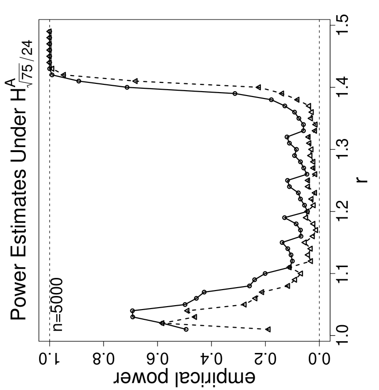
Figure 18: The empirical power estimates under association with $\varepsilon=5\sqrt{3}/24,\varepsilon=\sqrt{3}/12$ and $n=1000$ (left), $n=2000$ (middle), and $n=5000$ (right). The power estimates based on the binomial distribution are plotted in circles ($\circ$) and joined with solid lines, and those based on the normal approximation are plotted in triangles ($\triangle$) and joined with dashed lines.

The empirical power estimates for $r=3/2$ and $M=M_{C}$ are presented in Table 4.

Empirical Size and Power Estimates for $r=3/2$ and $M=M_{C}$
$n$	$\widehat{\alpha}^{S}$	$\widehat{\alpha}^{A}$	$\widehat{\beta}^{S}_{1}$	$\widehat{\beta}^{S}_{2}$	$\widehat{\beta}^{S}_{3}$	$\widehat{\beta}^{A}_{1}$	$\widehat{\beta}^{A}_{2}$	$\widehat{\beta}^{A}_{3}$
500	0.161	0.062	0.961	1.000	1.000	1.000	1.000	0.997
1000	0.071	0.082	0.975	1.000	1.000	1.000	1.000	1.000
2000	0.049	0.081	0.995	1.000	1.000	1.000	1.000	1.000

Table 4: The empirical size and power estimates for $r=3/2$ and $M=M_{C}$ under the null and alternatives. $n$ stands for size of $\mathcal{X}$ points, $\widehat{\alpha}^{S}$ for empirical size relative segregation, $\widehat{\alpha}^{A}$ for empirical size relative to association, $\widehat{\beta}^{S}_{1}$, $\widehat{\beta}^{S}_{2}$, and $\widehat{\beta}^{S}_{3}$ for empirical power estimates under $H^{S}_{\varepsilon}$ with $\varepsilon=\sqrt{3}/8,\varepsilon=\sqrt{3}/4,$ and $\varepsilon=2\sqrt{3}/7$, respectively, $\widehat{\beta}^{A}_{1}$, $\widehat{\beta}^{A}_{2}$, and $\widehat{\beta}^{A}_{3}$ for empirical power estimates under $H^{A}_{\varepsilon}$ with $\varepsilon=5\sqrt{3}/24,\varepsilon=\sqrt{3}/12,$ and $\varepsilon=\sqrt{3}/21$, respectively.

6 Correction for $\mathcal{X}$ Points Outside the Convex Hull of $\mathcal{Y}_{m}$

Our null hypothesis in (4) is rather restrictive, in the sense that, it might not be that realistic to assume the support of $\mathcal{X}$ being $C_{H}(\mathcal{Y}_{m})$ in practice. Up to now, our inference is restricted to the $C_{H}(\mathcal{Y}_{m})$. However, crucial information from the data (hence power) might be lost since a substantial proportion of $\mathcal{X}$ points, denoted $\pi_{out}$, might fall outside the $C_{H}(\mathcal{Y}_{m})$. We investigate the effect of $\pi_{out}$ (or restriction to the $C_{H}(\mathcal{Y}_{m})$) on our tests and propose an empirical correction to mitigate this based on an extensive Monte Carlo simulation study.

We consider the following 6 cases to investigate how the removal of points outside $C_{H}(\mathcal{Y}_{m})$ affects the empirical size and power performance of the tests. We only consider $r=1.35$ and $r=1.5$ which have better size and power performances compared to others. In each case, at each Monte Carlo replication, we generate $\mathcal{X}_{n}$ and $\mathcal{Y}_{m}$ independently as random samples from $\mathcal{U}(\mathcal{S}_{X})$ and $\mathcal{U}(\mathcal{S}_{Y})$, respectively, for various values of $n$ and $m$ where $\mathcal{S}_{X}$ and $\mathcal{S}_{Y}$ are the support sets of $\mathcal{X}$ and $\mathcal{Y}$ points, respectively. We take $\mathcal{S}_{Y}=(0,1)\times(0,1)$ and manipulate $\mathcal{S}_{X}$ in each case to simulate CSR and various forms of deviations from CSR. We repeat the generation procedure $N_{mc}$ times for each combination of $m$ and $n$. At each Monte Carlo replication, we record the number of $\mathcal{X}$ points outside $C_{H}(\mathcal{Y}_{m})$ and the domination number, $\gamma_{m,n}(r)$.

• In this case, we also set $\mathcal{S}_{X}=(0,1)\times(0,1)$,

• $\mathcal{S}_{X}=(-\delta,1+\delta)\times(-\delta,1+\delta)$ for $\delta\in\{.1,.25,.5\}$,

• $\mathcal{S}_{X}=(0,1)\times(0,1+\delta)$ for $\delta\in\{.1,.25,.5\}$,

• $\mathcal{S}_{X}=(0,1)\times(\delta,1+\delta)$ for $\delta\in\{.1,.25,.5\}$.

• Given a realization of $\mathcal{Y}$ points, $\mathcal{Y}_{m}=\{\mathsf{y}_{1},\mathsf{y}_{2},\ldots,\mathsf{y}_{m}\}$, from $\mathcal{U}(\mathcal{S}_{Y}=(0,1)\times(0,1))$, $\mathcal{S}_{X}=[(-\delta,1+\delta)\times(-\delta,1+\delta)]\setminus\bigcup_{i=1}^{m}B(\mathsf{y}_{i},\varepsilon)$ with $\delta=\frac{1}{2\,\sqrt{\lambda}}=\frac{1}{2\,\sqrt{m}}$ which the expected interpoint distance in a homogeneous Poisson process with intensity (expected number of points per unit area) $\lambda$ (Dixon, 2002b ) and $\varepsilon=\delta/k$ for $k=1.5,2.0$,

• Given a realization of $\mathcal{Y}$ points, $\mathcal{Y}_{m}=\{\mathsf{y}_{1},\mathsf{y}_{2},\ldots,\mathsf{y}_{m}\}$, from $\mathcal{U}(\mathcal{S}_{Y})$, $\mathcal{S}_{X}=\bigcup_{i=1}^{m}B(\mathsf{y}_{i},\varepsilon)$ with $\varepsilon=\delta/k$, $\delta=\frac{1}{2\,\sqrt{m}}$, and $k=1.0,1.5$.

Notice that in Case 1 both $\mathcal{X}_{n}$ and $\mathcal{Y}_{m}$ have the same support. By construction the two classes follow CSR independence with very different relative abundances (i.e., number of $\mathcal{X}$ points being larger than number of $\mathcal{Y}$ points). In Cases 2 and 3 the support of $\mathcal{X}_{n}$ contains (but larger than) the support of $\mathcal{Y}_{m}$, which suggests segregation of $\mathcal{X}$ points from $\mathcal{Y}$ points, at least when we move away from the support of $\mathcal{Y}$ points (which is the unit square). However, when we restrict our attention to $C_{H}(\mathcal{Y}_{m})$ or the unit square, we have CSR or CSR independence, respectively. Furthermore, the larger the $\delta$ value, the larger the level of segregation of $\mathcal{X}$ from $\mathcal{Y}$. In Case 4 the support of $\mathcal{X}_{n}$ and $\mathcal{Y}_{m}$ overlap, but neither is a subset of the other, which suggests segregation between $\mathcal{X}$ and $\mathcal{Y}$ points. When we restrict our attention to $C_{H}(\mathcal{Y}_{m})$, there is still segregation between $\mathcal{X}$ and $\mathcal{Y}$ points. Furthermore, the larger the $\delta$ value, the larger the level of segregation between $\mathcal{X}$ and $\mathcal{Y}$ points. In Case 5, $\mathcal{X}$ points are segregated from $\mathcal{Y}$ points both in and outside $C_{H}(\mathcal{Y}_{m})$. Furthermore, the larger the $\delta$ value, the larger the level of segregation of $\mathcal{X}$ points from $\mathcal{Y}$ points. Finally, in Case 6 $\mathcal{X}$ points are associated with $\mathcal{Y}$ points. Furthermore, the smaller the $\delta$ value, the larger the level of association of $\mathcal{X}$ points with $\mathcal{Y}$ points.

In Case 1 (i.e., the benchmark case), we consider $n=100,200,\ldots,900,1000,2000,\ldots,9000,10000$ for each of $m=10,20,\ldots,50$. We generate $N_{mc}=1000$ replication for each $n,m$ combination. In the other cases, we consider $n=100,500,1000$ for $m=10$ and $n=500,1000$ for $m=20$; and we generate $N_{mc}=10000$ replication for each $n,m$ combination.

In Cases 1-6, we estimate the proportion of $\mathcal{X}$ points outside the $C_{H}(\mathcal{Y}_{m})$. For each $m,n$ combination we average (over $n$) this proportion which is denoted as $\widehat{\pi}_{out}$. We present the estimated (mean) proportions $\widehat{\pi}_{out}$ for Case 1 in Table 5 and for Cases 2-6 in Table 6. Observe that in Cases 2-5, $\widehat{\pi}_{out}$ values are larger than that in Case 1, while in Case 6, $\widehat{\pi}_{out}$ values are smaller than that in Case 1.

$m$	10	20	30	40	50
$\widehat{\pi}_{out}$	0.56	0.37	0.29	0.23	0.20
$\widehat{\pi}_{fit}$	0.57	0.36	0.28	0.24	0.21

Table 5: The (mean) proportion of $\mathcal{X}$ points outside the $C_{H}(\mathcal{Y}_{m})$ which is denoted as $\widehat{\pi}_{out}$ and the fitted values $\widehat{\pi}_{fit}$ for various $m$ values in Case 1.

$\widehat{\pi}_{out}$ values for Case 2
$\delta$	0.1	0.25	0.50
$m=10$	0.697	0.806	0.891
$m=20$	0.566	0.722	0.843

$\widehat{\pi}_{out}$ values for Case 3
$\delta$	0.1	0.25	0.50
$m=10$	0.604	0.652	0.740
$m=20$	0.431	0.499	0.582

$\widehat{\pi}_{out}$ values for Case 4
$\delta$	0.1	0.25	0.50
$m=10$	0.573	0.629	0.782
$m=20$	0.395	0.488	0.687

$\widehat{\pi}_{out}$ values for Case 5
$k$	1.5	2.0
$m=10$	0.806	0.783
$m=20$	0.652	0.611

$\widehat{\pi}_{out}$ values for Case 6
$k$	1.0	1.5
$m=10$	0.535	0.479
$m=20$	0.358	0.310

Table 6: The (mean) proportion of $\mathcal{X}$ points outside the $C_{H}(\mathcal{Y}_{m})$ for various $\delta$ and $m$ values in Cases 2-4 and various $k$ and $m$ values in Cases 5-6.

For Case 1, we model the relationship between $\widehat{\pi}_{out}$ and $m$. Our simulation results suggest that $\widehat{\pi}_{out}\approx 1.7932/m+1.2229/\sqrt{m}$. We present the actual fitted values denoted $\widehat{\pi}_{fit}$ based on this model in Table 5. See also Figure 19 for the plot of estimated $\widehat{\pi}_{out}$ values versus fitted values based on our model. Notice that as $m\rightarrow\infty$, $\widehat{\pi}_{out}\rightarrow 0$.

Figure 19: The proportion of $X$ points outside $C_{H}(\mathcal{Y}_{m})$ as a function of $m$. The solid line is the fitted line based on $\pi_{out}\approx 1.7932/m+1.2229/\sqrt{m}$.

Based on our Monte Carlo simulation results we propose a coefficient to adjust for the proportion of $\mathcal{X}$ points outside $C_{H}(\mathcal{Y}_{m})$, namely,

$$C_{ch}:=1-(p_{out}-\mathbf{E}\,[\widehat{\pi}_{out}])$$ (12)

where $p_{out}$ is the observed and $\mathbf{E}\,[\widehat{\pi}_{out}]\approx 1.7932/m+1.2229/\sqrt{m}$ is the expected (under the conditions stated in Case 1) proportion of $\mathcal{X}$ points outside $C_{H}(\mathcal{Y}_{m})$. For the binomial test statistic in Equation (10), we suggest

$$B^{ch}_{n,m}:=\left\{\begin{array}[]{ll}(\gamma_{n}(r,M)-2J_{m})\cdot C_{ch}=(\sum_{j=1}^{J_{m}}\gamma_{{}_{[j]}}(r)-2J_{m})\cdot C_{ch}&\text{if $\gamma_{n}(r,M)\cdot C_{ch}>2J_{m}$,}\\ 0&\text{otherwise.}\\ \end{array}\right.$$ (13)

For the mean domination number (per triangle) of the PCD, we suggest

$$S^{ch}_{n,m}=S_{n,m}\cdot C_{ch}.$$ (14)

This (convex hull) adjustment slightly affects the empirical size estimates in Case 1, since $p_{out}$ and $\mathbf{E}\,[\widehat{\pi}_{out}]$ values are very similar. In Cases 2-5, there is segregation when all data points are considered, and $p_{out}$ values tend to be larger than $\mathbf{E}\,[\widehat{\pi}_{out}]$ values, and in Case 6 (which is the simulation of the association case), $p_{out}$ values tend to be smaller than $\mathbf{E}\,[\widehat{\pi}_{out}]$ values. Hence in Cases 2-6, the adjustment seems to correct the power estimates in the desired direction, thereby increasing the power estimates.

7 Correction for Small Samples

The distributional results in Equations (2) and (5) might require large $n$ for the convergence to hold. In particular, it might be necessary for the number of $\mathcal{X}$ points per Delaunay triangle to be larger than 100 as a practical guide which implies very large samples from $\mathcal{X}$ are needed for a large number of $\mathcal{Y}$ points. Hence it might be necessary to propose a correction in the test statistics for small $n$ also. Based on our extensive Monte Carlo simulations (of Case 1 above) we suggest that the test statistic $S_{n,m}$ in Equation (11) can be adjusted as $S^{adj}_{n,m}:=\frac{S_{n,m}-a_{n,m}}{b_{n,m}}$. We provide the explicit forms of $a_{n,m}$ and $b_{n,m}$ for $m=10,20,\ldots,50$ in Table 7. For example for $m=10$, $S_{n,m}$ in Equation (11) can be adjusted as $S^{adj}_{n,m}:=\frac{S_{n,m}-a_{n,m}}{b_{n,m}}$ where $a_{n,m}=-8.80/(n/J_{m})-30.94/\sqrt{n/J_{m}}+9.09/\sqrt[3]{n/J_{m}}$ and $b_{n}=1-18.81/(n/J_{m})+16.26/\sqrt{n/J_{m}}-4.42/\sqrt[3]{n/J_{m}}$. Observe that as expected $S^{adj}_{n,m}$ converges to $S_{n,m}$ as $n\rightarrow\infty$ for each $m$ value considered provided $n/J_{m}\rightarrow\infty$ which is a requirement in our testing framework.

$r=1.5$
$m$	$a_{n,m}$	$b_{n,m}$
10	$-8.80/(n/J_{m})-30.94/\sqrt{n/J_{m}}+9.09/\sqrt[3]{n/J_{m}}$	$1-18.81/(n/J_{m})+16.26/\sqrt{n/J_{m}}-4.42/\sqrt[3]{n/J_{m}}$
20	$10.19/(n/J_{m})-58.15/\sqrt{n/J_{m}}+20.27/\sqrt[3]{n/J_{m}}$	$1-11.16/(n/J_{m})+11.71/\sqrt{n/J_{m}}-3.24/\sqrt[3]{n/J_{m}}$
30	$18.72/(n/J_{m})-77.36/\sqrt{n/J_{m}}+28.46/\sqrt[3]{n/J_{m}}$	$1-6.85/(n/J_{m})+7.56/\sqrt{n/J_{m}}-1.62/\sqrt[3]{n/J_{m}}$
40	$28.11/(n/J_{m})-99.66/\sqrt{n/J_{m}}+38.73/\sqrt[3]{n/J_{m}}$	$1-5.23/(n/J_{m})+5.81/\sqrt{n/J_{m}}-0.92/\sqrt[3]{n/J_{m}}$
50	$33.37/(n/J_{m})-115.58/\sqrt{n/J_{m}}+46.03/\sqrt[3]{n/J_{m}}$	$1-3.93/(n/J_{m})+3.88/\sqrt{n/J_{m}}+0.03/\sqrt[3]{n/J_{m}}$
$r=1.35$
$m$	$a_{n,m}$	$b_{n,m}$
10	$-0.13/(n/J_{m})-34.35/\sqrt{n/J_{m}}+8.79/\sqrt[3]{n/J_{m}}$	$1-16.29/(n/J_{m})+13.43/\sqrt{n/J_{m}}-3.43/\sqrt[3]{n/J_{m}}$
20	$16.05/(n/J_{m})-58.95/\sqrt{n/J_{m}}+18.01/\sqrt[3]{n/J_{m}}$	$1-10.49/(n/J_{m})+10.70/\sqrt{n/J_{m}}-3.04/\sqrt[3]{n/J_{m}}$
30	$24.22/(n/J_{m})-77.98/\sqrt{n/J_{m}}+25.78/\sqrt[3]{n/J_{m}}$	$1-5.59/(n/J_{m})+5.52/\sqrt{n/J_{m}}-0.82/\sqrt[3]{n/J_{m}}$
40	$30.66/(n/J_{m})-95.07/\sqrt{n/J_{m}}+32.91/\sqrt[3]{n/J_{m}}$	$1-4.02/(n/J_{m})+3.57/\sqrt{n/J_{m}}-0.06/\sqrt[3]{n/J_{m}}$
50	$34.49/(n/J_{m})-107.87/\sqrt{n/J_{m}}+38.18/\sqrt[3]{n/J_{m}}$	$1-3.07/(n/J_{m})+2.55/\sqrt{n/J_{m}}+0.42/\sqrt[3]{n/J_{m}}$

Table 7: The finite sample adjustment for $S_{n,m}$ in Equation (11) as $S^{adj}_{n,m}:=\frac{S-a_{n,m}}{b_{n,m}}$ with $m=10,20,\ldots,50$ and $n=100,200,\ldots,1000,2000,\ldots,10000$ for $r=1.5$ (top) and $r=1.35$ (bottom).

8 Extension of $N_{PE}^{r}$ to Higher Dimensions:

The extension to $\mathbb{R}^{d}$ for $d>2$ with $M=M_{C}$ is provided in (Ceyhan and Priebe, (2005)), the extension for general $M$ is similar: Let $\mathcal{Y}=\{\mathsf{y}_{1},\mathsf{y}_{2},\cdots,\mathsf{y}_{d+1}\}$ be $d+1$ non-coplanar points. Denote the simplex formed by these $d+1$ points as $\mathcal{S}(\mathcal{Y})$. For $r\in[1,\infty]$, define the $r$-factor proximity map as follows. Given a point $x$ in $\mathcal{S}(\mathcal{Y})$, let $Q_{\mathsf{y}}(M,x)$ be the polytope with vertices being the $d\,(d+1)/2$ points on the edges, the vertex $\mathsf{y}$ and $x$ so that the faces of $Q_{\mathsf{y}}(M,x)$ are formed by $d-1$ line segments each of which joining one of $\mathcal{Y}$ points, say $\mathsf{y}_{i}$, to $M$ and that are between $M$ and the face opposite $\mathsf{y}_{i}$. That is, the vertex region for vertex $v$ is the polytope with vertices given by $v$ and such points on the edges. Let $v(x)$ be the vertex in whose region $x$ falls. If $x$ falls on the boundary of two vertex regions, we assign $v(x)$ arbitrarily. Let $\varphi(x)$ be the face opposite to vertex $v(x)$, and $\eta(v(x),x)$ be the hyperplane parallel to $\varphi(x)$ which contains $x$. Let $d(v(x),\eta(v(x),x))$ be the (perpendicular) Euclidean distance from $v(x)$ to $\eta(v(x),x)$. For $r\in[1,\infty)$, let $\eta_{r}(v(x),x)$ be the hyperplane parallel to $\varphi(x)$ such that $d(v(x),\eta_{r}(v(x),x))=r\,d(v(x),\eta(v(x),x))$ and $d(\eta(v(x),x),\eta_{r}(v(x),x))<d(v(x),\eta_{r}(v(x),x))$. Let $\mathcal{S}_{r}(x)$ be the polytope similar to and with the same orientation as $\mathcal{S}(\mathcal{Y})$ having $v(x)$ as a vertex and $\eta_{r}(v(x),x)$ as the opposite face. Then the $r$-factor proximity region $N_{\mathcal{Y}}^{r}(x):=\mathcal{S}_{r}(x)\cap\mathcal{S}(\mathcal{Y})$. Also, let $\zeta_{j}(x)$ be the hyperplane such that $\zeta_{j}(x)\cap\mathcal{S}(\mathcal{Y})\not=\emptyset$ and $r\,d(\mathsf{y}_{j},\zeta_{j}(x))=d(\mathsf{y}_{j},\eta(\mathsf{y}_{j},x))$ for $j=1,2,\ldots,d+1$. Then the $\Gamma_{1}$-region is $\Gamma^{r}_{1}(x)=\bigcup_{j=1}^{d+1}(\Gamma^{r}_{1}(x)\cap R_{M}(\mathsf{y}_{j}))$ where $\Gamma^{r}_{1}(x)\cap R_{M}(\mathsf{y}_{j})=\{z\in R_{M}(\mathsf{y}_{j}):d(\mathsf{y}_{j},\eta(\mathsf{y}_{j},z))\geq d(\mathsf{y}_{j},\zeta_{j}(x)\}$, for $j=1,2,\ldots,d+1$.

Let $X_{\varphi}:=\operatorname{argmin}_{X\in\mathcal{X}_{n}}d(X,\varphi)$ be the closest point among $\mathcal{X}_{n}$ to face $\varphi$. Then it is easily seen that $\Gamma^{r}_{1}(\mathcal{X}_{n},M)=\bigcap_{i=1}^{d+1}\Gamma^{r}_{1}(X_{\varphi_{i}},M)$, where $\varphi_{i}$ is the face opposite vertex $\mathsf{y}_{i}$, for $i=1,2,\ldots,d$. So $\Gamma^{r}_{1}(\mathcal{X}_{n},M)\cap R_{M}(\mathsf{y}_{i})=\{z\in R_{M}(\mathsf{y}_{i}):\;d(\mathsf{y}_{i},\eta(\mathsf{y}_{i},z)\geq d(\mathsf{y}_{i},\Xi_{i}(X_{\varphi_{i}}))\}$, for $i=1,2,\ldots,d$.

Let the domination number be $\gamma_{n}(r,F,M,d):=\gamma_{n}(\mathcal{X}_{n};F,N_{PE}^{r},d)$ and $X_{[i,1]}:=\operatorname{argmin}_{X\in\mathcal{X}_{n}\cap R_{M}(\mathsf{y}_{i})}d(X,\varphi_{i})$. Then $\gamma_{n}(r,M)\leq d+1$ with probability 1, since $\mathcal{X}_{n}\cap R_{M}(\mathsf{y}_{i})\subset N_{PE}^{r}\left(X_{[i,1]},M\right)$ for each of $i=1,2,\ldots,d$.

In $\mathcal{S}(\mathcal{Y})$, drawing the hyper-surfaces $Q_{i}(r,x)$ such that $d(\mathsf{y}_{i},\varphi_{i})=r\,d(\mathsf{y}_{i},Q_{i}(r,x))$ for $i\in\{1,2,\ldots,d\}$ yields another polytope, denoted as $\mathscr{P}_{r}$, for $r<(d+1)/d$. Let $\gamma_{n}(r,M,d):=\gamma(\mathcal{X}_{n},N_{PE}^{r},M,d)$ be the domination number of the PCD based on the extension of $N_{PE}^{r}(\cdot,M)$ to $\mathbb{R}^{d}$. Then we conjecture the following:

Conjecture 8.1.

Suppose $\mathcal{X}_{n}$ is set of iid random variables from the uniform distribution on a simplex in $\mathbb{R}^{d}$. Then as $n\rightarrow\infty$, the domination number $\gamma_{n}(r,M,d)$ in the simplex satisfies

$$\gamma_{n}(r,M,d)\stackrel{{\scriptstyle\mathcal{L}}}{{\longrightarrow}}\left\{\begin{array}[]{ll}d+\operatorname{BER}(1-p_{r,d})&\text{for $r\in[1,(d+1)/d)$ and $M\in\{t_{1}(r),t_{2}(r),\ldots,t_{d+1}(r)\}$,}\\ \leq(d-1)&\text{for $r>(d+1)/d$ and $M\in\mathcal{S}(\mathcal{Y})^{o}$,}\\ d+1&\text{for $r\in[1,(d+1)/d)$ and $M\in\mathscr{P}_{r}\setminus\{t_{1}(r),t_{2}(r),\ldots,t_{d+1}(r)\}$,}\\ \end{array}\right.$$ (15)

where $p_{r,d}$ can be calculated by intensive numerical integration as in the calculation of Equation (3) and for $r=(d+1)/d$ and $M=M_{C}$, $p_{r,d}$ will be different from the continuous extension of Equation (15).

9 Discussion and Conclusions

In this article, we consider the asymptotic distribution of the domination number of proportional-edge proximity catch digraphs (PCDs), for testing bivariate spatial point patterns of segregation and association. To our knowledge the PCD-based methods are the only graph theoretic methods for testing spatial patterns in literature (Ceyhan and Priebe, (2005), Ceyhan et al., (2006), and Ceyhan et al., (2007)). The new PCDs when compared to class cover catch digraphs (CCCDs), have some advantages. In particular, the asymptotic distribution of the domination number $\gamma_{n}(r,M)$ of the proportional-edge PCDs, unlike that of CCCDs, is mathematically tractable (although computable by numerical integration). A minimum dominating set can be found in polynomial time for proportional-edge PCDs in $\mathbb{R}^{d}$ for all $d\geq 1$, but finding a minimum dominating set is an NP-hard problem for CCCDs (except for $\mathbb{R}$). These nice properties of proportional-edge PCDs are due to the geometry invariance of distribution of $\gamma_{n}(r,M)$ for uniform data in triangles.

On the other hand, CCCDs are easily extendable to higher dimensions and are defined for all $\mathcal{X}_{n}\subset\mathbb{R}^{d}$, while proportional-edge PCDs are only defined for $\mathcal{X}_{n}\subset\mathcal{C}_{H}(\mathcal{Y}_{m})$. Furthermore, the CCCDs based on balls use proximity regions that are defined by the obvious metric, while the PCDs in general do not suggest a metric. In particular, our proportional-edge PCDs are based on some sort of dissimilarity measure, but not a metric.

The finite sample distribution of $\gamma_{n}(r,M)$, although computationally tedious, can be found by numerical methods, while that of CCCDs can only be empirically estimated by Monte Carlo simulations. Moreover, we had to introduce many auxiliary tools to compute the distribution of $\gamma_{n}(r,M)$ in $\mathbb{R}^{2}$. Same tools will work in higher dimensions, perhaps with more complicated geometry. The proportional-edge PCDs lend themselves for such a purpose, because of the geometry invariance property for uniform data on Delaunay triangles. Let the two samples of sizes $n$ and $m$ be from classes $\mathcal{X}$ and $\mathcal{Y}$, respectively, with $\mathcal{X}$ points being used as the vertices of the PCDs and $\mathcal{Y}$ points being used in the construction of Delaunay triangulation. For the domination number approach to be appropriate, $n$ should be much larger compared to $m$. This implies that $n$ tends to infinity while $m$ is assumed to be fixed. That is, the imbalance in the relative abundance of the two classes should be large for this method. Such an imbalance usually confounds the results of other spatial interaction tests. Furthermore, we can also use the normal approximation to binomial distribution for the domination number, provided $n$ is much larger than $m$, but both sizes tending to infinity. Therefore, as long as $n\gg m\rightarrow\infty$, we can remove the conditioning on $m$.

The null hypothesis is assumed to be CSR of $\mathcal{X}$ points, i.e., the uniformness of $\mathcal{X}$ points in the convex hull of $\mathcal{Y}$ points. Although we have two classes here, the null pattern is not the CSR independence, since for finite $m$, we condition on $m$ and the locations of the $\mathcal{Y}$ points are irrelevant as long as they are not co-circular. That is, the $\mathcal{Y}$ points can result from any pattern that results in a unique Delaunay triangulation. When $m\rightarrow\infty$, conditioning on $m$ does not persist.

There are many types of parametrizations for the alternatives. The particular parametrization of the alternatives in Equation (6) is chosen so that the distribution of the domination number under the alternatives would be geometry invariant (i.e., independent of the geometry of the support triangles). The more natural alternatives (i.e., the alternatives that are more likely to be found in practice) can be similar to or might be approximated by our parametrization. Because in any segregation alternative, the $\mathcal{X}$ points will tend to be further away from $\mathcal{Y}$ points and in any association alternative $\mathcal{X}$ points will tend to cluster around the $\mathcal{Y}$ points. And such patterns can be detected by the test statistics based on the domination number, since under segregation (whether it is parametrized as in Section 4 or not) we expect them to be smaller, and under association (regardless of the parametrization) they tend to be larger.

By construction our method uses only the $\mathcal{X}$ points in $C_{H}(\mathcal{Y}_{m})$ (the convex hull of $\mathcal{Y}$ points) which might cause substantial data (hence information) loss. To mitigate this, we propose a correction for the proportion of $\mathcal{X}$ points outside $C_{H}(\mathcal{Y}_{m})$, because the pattern inside $C_{H}(\mathcal{Y}_{m})$ might not be the same as the pattern outside $C_{H}(\mathcal{Y}_{m})$. We suggest analysis with our domination number approach in two steps: (i) analysis restricted to $C_{H}(\mathcal{Y}_{m})$, which provides inference only for $\mathcal{X}$ points in $C_{H}(\mathcal{Y}_{m})$, (ii) overall analysis with convex hull correction (i.e., for all $\mathcal{X}$ points with respect to $\mathcal{Y}_{m}$). When the number of Delaunay triangles based on $\mathcal{Y}$ points, denoted $J_{m}$, is less than 30, we recommend the use of binomial distribution as $n\rightarrow\infty$ (i.e., for large $n$); when $J_{m}$ is larger than 30, we recommend the use of normal approximation as $n\rightarrow\infty$. For small samples, one might use Monte Carlo simulation or randomization with our approach or apply a finite sample correction as in Section 7. In the case of small samples with some $\mathcal{X}$ points existing outside $C_{H}(\mathcal{Y}_{m})$, convex hull correction can be implemented first, and then the small sample correction. Furthermore, when testing against segregation we recommend the parameter $r\approx 1.3$, while for testing against association we recommend the parameter $r\approx 1.35$ as they exhibit the best performance in terms of size and power. The proportional-edge PCDs have applications in classification. This can be performed building discriminant regions in a manner analogous to the procedure proposed in Priebe et al., 2003a .

References

- Baddeley et al., (2000) Baddeley, A., Møller, J., and Waagepetersen, R. (2000). Non- and semi-parametric estimation of interaction in inhomogeneous point patterns. Statistica Neerlandica, 54(3):329–350.
- Ceyhan, (2005) Ceyhan, E. (2005). An Investigation of Proximity Catch Digraphs in Delaunay Tessellations, also available as technical monograph titled “Proximity Catch Digraphs: Auxiliary Tools, Properties, and Applications” by VDM Verlag, ISBN: 978-3-639-19063-2. PhD thesis, The Johns Hopkins University, Baltimore, MD, 21218.
- Ceyhan, (2008) Ceyhan, E. (2008). The distribution of the domination number of class cover catch digraphs for non-uniform one-dimensional data. Discrete Mathematics, 308:5376–5393.
- Ceyhan and Priebe, (2003) Ceyhan, E. and Priebe, C. (2003). Central similarity proximity maps in Delaunay tessellations. In Proceedings of the Joint Statistical Meeting, Statistical Computing Section, American Statistical Association.
- Ceyhan and Priebe, (2005) Ceyhan, E. and Priebe, C. E. (2005). The use of domination number of a random proximity catch digraph for testing spatial patterns of segregation and association. Statistics & Probability Letters, 73:37–50.
- Ceyhan and Priebe, (2007) Ceyhan, E. and Priebe, C. E. (2007). On the distribution of the domination number of a new family of parametrized random digraphs. Model Assisted Statistics and Applications, 1(4):231–255.
- Ceyhan et al., (2007) Ceyhan, E., Priebe, C. E., and Marchette, D. J. (2007). A new family of random graphs for testing spatial segregation. Canadian Journal of Statistics, 35(1):27–50.
- Ceyhan et al., (2006) Ceyhan, E., Priebe, C. E., and Wierman, J. C. (2006). Relative density of the random -factor proximity catch digraphs for testing spatial patterns of segregation and association. Computational Statistics & Data Analysis, 50(8):1925–1964.
- Chartrand and Lesniak, (1996) Chartrand, G. and Lesniak, L. (1996). Graphs & Digraphs. Chapman & Hall/CRC Press LLC, Florida.
- Coomes et al., (1999) Coomes, D. A., Rees, M., and Turnbull, L. (1999). Identifying aggregation and association in fully mapped spatial data. Ecology, 80(2):554–565.
- Cuzick and Edwards, (1990) Cuzick, J. and Edwards, R. (1990). Spatial clustering for inhomogeneous populations (with discussion). Journal of the Royal Statistical Society, Series B, 52:73–104.
- DeVinney and Priebe, (2006) DeVinney, J. and Priebe, C. E. (2006). A new family of proximity graphs: Class cover catch digraphs. Discrete Applied Mathematics, 154(14):1975–1982.
- DeVinney et al., (2002) DeVinney, J., Priebe, C. E., Marchette, D. J., and Socolinsky, D. (2002). Random walks and catch digraphs in classification. http://www.galaxy.gmu.edu/interface/I02/I2002Proceedings/DeVinneyJason/%DeVinneyJason.paper.pdf. Proceedings of the Symposium on the Interface: Computing Science and Statistics, Vol. 34.
- DeVinney and Wierman, (2003) DeVinney, J. and Wierman, J. C. (2003). A SLLN for a one-dimensional class cover problem. Statistics & Probability Letters, 59(4):425–435.
- Diggle, (2003) Diggle, P. J. (2003). Statistical Analysis of Spatial Point Patterns. Hodder Arnold Publishers, London.
- Dixon, (1994) Dixon, P. M. (1994). Testing spatial segregation using a nearest-neighbor contingency table. Ecology, 75(7):1940–1948.
- (17) Dixon, P. M. (2002a). Nearest-neighbor contingency table analysis of spatial segregation for several species. Ecoscience, 9(2):142–151.
- (18) Dixon, P. M. (2002b). Nearest neighbor methods. Encyclopedia of Environmetrics, edited by Abdel H. El-Shaarawi and Walter W. Piegorsch, John Wiley & Sons Ltd., NY, 3:1370–1383.
- Eeden, (1963) Eeden, C. V. (1963). The relation between Pitman’s asymptotic relative efficiency of two tests and the correlation coefficient between their test statistics. The Annals of Mathematical Statistics, 34(4):1442–1451.
- Fall et al., (2007) Fall, A., Fortin, M. J., Manseau, M., and O’Brien, D. (2007). Ecosystems. International Journal of Geographical Information Science, 10(3):448–461.
- Friedman and Rafsky, (1983) Friedman, J. H. and Rafsky, L. C. (1983). Graph-theoretic measures of multivariate association and prediction. The Annals of Statistics, 11(2):377–391.
- Hamill and Wright, (1986) Hamill, D. M. and Wright, S. J. (1986). Testing the dispersion of juveniles relative to adults: A new analytical method. Ecology, 67(2):952–957.
- Hodges and Lehmann, (1956) Hodges, J. L. J. and Lehmann, E. L. (1956). The efficiency of some nonparametric competitors of the -test. The Annals of Mathematical Statistics, 27(2):324–335.
- Jaromczyk and Toussaint, (1992) Jaromczyk, J. W. and Toussaint, G. T. (1992). Relative neighborhood graphs and their relatives. Proceedings of IEEE, 80:1502–1517.
- Keitt, (2007) Keitt, T. (2007). Introduction to spatial modeling with networks. Presented at the Workshop on Networks in Ecology and Beyond Organized by the PRIMES (Program in Interdisciplinary Math, Ecology and Statistics) at Colorado State University, Fort Collins, Colorado.
- Kendall and Stuart, (1979) Kendall, M. and Stuart, A. (1979). The Advanced Theory of Statistics, Volume 2, 4th edition. Griffin, London.
- Kulldorff, (2006) Kulldorff, M. (2006). Tests for spatial randomness adjusted for an inhomogeneity: A general framework. Journal of the American Statistical Association, 101(475):1289–1305.
- Lee, (1998) Lee, C. (1998). Domination in digraphs. Journal of Korean Mathematical Society, 4:843–853.
- Marchette and Priebe, (2003) Marchette, D. J. and Priebe, C. E. (2003). Characterizing the scale dimension of a high dimensional classification problem. Pattern Recognition, 36(1):45–60.
- Minor and Urban, (2007) Minor, E. S. and Urban, D. L. (2007). Graph theory as a proxy for spatially explicit population models in conservation planning. Ecological Applications, 17(6):1771–1782.
- Nanami et al., (1999) Nanami, S. H., Kawaguchi, H., and Yamakura, T. (1999). Dioecy-induced spatial patterns of two codominant tree species, Podocarpus nagi and Neolitsea aciculata. Journal of Ecology, 87(4):678–687.
- Okabe et al., (2000) Okabe, A., Boots, B., Sugihara, K., and Chiu, S. N. (2000). Spatial Tessellations: Concepts and Applications of Voronoi Diagrams. Wiley.
- Paterson and Yao, (1992) Paterson, M. S. and Yao, F. F. (1992). On nearest neighbor graphs. In Proceedings of Int. Coll. Automata, Languages and Programming, Springer LNCS, volume 623, pages 416–426.
- Perry et al., (2006) Perry, G., Miller, B., and Enright, N. (2006). A comparison of methods for the statistical analysis of spatial point patterns in plant ecology. Plant Ecology, 187(1):59 –82.
- Pielou, (1961) Pielou, E. C. (1961). Segregation and symmetry in two-species populations as studied by nearest-neighbor relationships. Journal of Ecology, 49(2):255–269.
- Priebe et al., (2001) Priebe, C. E., DeVinney, J. G., and Marchette, D. J. (2001). On the distribution of the domination number of random class cover catch digraphs. Statistics & Probability Letters, 55:239–246.
- (37) Priebe, C. E., Marchette, D. J., DeVinney, J., and Socolinsky, D. (2003a). Classification using class cover catch digraphs. Journal of Classification, 20(1):3–23.
- (38) Priebe, C. E., Solka, J. L., Marchette, D. J., and Clark, B. T. (2003b). Class cover catch digraphs for latent class discovery in gene expression monitoring by DNA microarrays. Computational Statistics & Data Analysis on Visualization, 43-4:621–632.
- Ripley, (2004) Ripley, B. D. (2004). Spatial Statistics. Wiley-Interscience, New York.
- Roberts et al., (2000) Roberts, S. A., Hall, G. B., and Calamai, P. H. (2000). Analysing forest fragmentation using spatial autocorrelation, graphs and GIS. International Journal of Geographical Information Science, 14(2):185–204.
- Stoyan and Penttinen, (2000) Stoyan, D. and Penttinen, A. (2000). Recent applications of point process methods in forestry statistics. Statistical Science, 15(1):61–78.
- Su et al., (2007) Su, W. Z., Yang, G. S., Yao, S. M., and Yang, Y. B. (2007). Scale-free structure of town road network in southern Jiangsu Province of China. Chinese Geographical Science, 17(4):311–316.
- Toussaint, (1980) Toussaint, G. T. (1980). The relative neighborhood graph of a finite planar set. Pattern Recognition, 12(4):261–268.
- West, (2001) West, D. B. (2001). Introduction to Graph Theory, Edition. Prentice Hall, NJ.
- Wierman and Xiang, (2008) Wierman, J. C. and Xiang, P. (2008). A general SLLN for the one-dimensional class cover problem. Statistics & Probability Letters, 78(9):1110–1118.
- Wu and Murray, (2008) Wu, X. and Murray, A. T. (2008). A new approach to quantifying spatial contiguity using graph theory and spatial interaction. International Journal of Geographical Information Science, 22(4):387–407.
- Xiang and Wierman, (2009) Xiang, P. and Wierman, J. C. (2009). A CLT for a one-dimensional class cover problem. Statistics & Probability Letters, 79(2):223–233.