Measurement of dijet photoproduction for
events with a leading neutron
at HERA
Abstract
Differential cross sections for dijet photoproduction and this process in association with a leading neutron, , have been measured with the ZEUS detector at HERA using an integrated luminosity of 40 pb-1. The fraction of dijet events with a leading neutron was studied as a function of different jet and event variables. Single- and double-differential cross sections are presented as a function of the longitudinal fraction of the proton momentum carried by the leading neutron, , and of its transverse momentum squared, . The dijet data are compared to inclusive DIS and photoproduction results; they are all consistent with a simple pion-exchange model. The neutron yield as a function of was found to depend only on the fraction of the proton beam energy going into the forward region, independent of the hard process. No firm conclusion can be drawn on the presence of rescattering effects.
DESY–09–139
The ZEUS Collaboration
S. Chekanov,
M. Derrick,
S. Magill,
B. Musgrave,
D. Nicholass1,
J. Repond,
R. Yoshida
Argonne National Laboratory, Argonne, Illinois 60439-4815, USA n
M.C.K. Mattingly
Andrews University, Berrien Springs, Michigan 49104-0380, USA
P. Antonioli,
G. Bari,
L. Bellagamba,
D. Boscherini,
A. Bruni,
G. Bruni,
F. Cindolo,
M. Corradi,
G. Iacobucci,
A. Margotti,
R. Nania,
A. Polini
INFN Bologna, Bologna, Italy e
S. Antonelli,
M. Basile,
M. Bindi,
L. Cifarelli,
A. Contin,
S. De Pasquale2,
G. Sartorelli,
A. Zichichi
University and INFN Bologna, Bologna, Italy e
D. Bartsch,
I. Brock,
H. Hartmann,
E. Hilger,
H.-P. Jakob,
M. Jüngst,
A.E. Nuncio-Quiroz,
E. Paul,
U. Samson,
V. Schönberg,
R. Shehzadi,
M. Wlasenko
Physikalisches Institut der Universität Bonn,
Bonn, Germany b
J.D. Morris3
H.H. Wills Physics Laboratory, University of Bristol,
Bristol, United Kingdom m
M. Kaur,
P. Kaur4,
I. Singh4
Panjab University, Department of Physics, Chandigarh, India
M. Capua,
S. Fazio,
A. Mastroberardino,
M. Schioppa,
G. Susinno,
E. Tassi5
Calabria University,
Physics Department and INFN, Cosenza, Italy e
J.Y. Kim6
Chonnam National University, Kwangju, South Korea
Z.A. Ibrahim,
F. Mohamad Idris,
B. Kamaluddin,
W.A.T. Wan Abdullah
Jabatan Fizik, Universiti Malaya, 50603 Kuala Lumpur, Malaysia r
Y. Ning,
Z. Ren,
F. Sciulli
Nevis Laboratories, Columbia University, Irvington on Hudson,
New York 10027, USA o
J. Chwastowski,
A. Eskreys,
J. Figiel,
A. Galas,
K. Olkiewicz,
B. Pawlik,
P. Stopa,
L. Zawiejski
The Henryk Niewodniczanski Institute of Nuclear Physics, Polish Academy of Sciences, Cracow,
Poland i
L. Adamczyk,
T. Bołd,
I. Grabowska-Bołd,
D. Kisielewska,
J. Łukasik7,
M. Przybycień,
L. Suszycki
Faculty of Physics and Applied Computer Science,
AGH-University of Science and Technology, Cracow, Poland p
A. Kotański8,
W. Słomiński9
Department of Physics, Jagellonian University, Cracow, Poland
O. Bachynska,
O. Behnke,
J. Behr,
U. Behrens,
C. Blohm,
K. Borras,
D. Bot,
R. Ciesielski,
N. Coppola,
S. Fang,
A. Geiser,
P. Göttlicher10,
J. Grebenyuk,
I. Gregor,
T. Haas,
W. Hain,
A. Hüttmann,
F. Januschek,
B. Kahle,
I.I. Katkov11,
U. Klein12,
U. Kötz,
H. Kowalski,
V. Libov,
M. Lisovyi,
E. Lobodzinska,
B. Löhr,
R. Mankel13,
I.-A. Melzer-Pellmann,
S. Miglioranzi14,
A. Montanari,
T. Namsoo,
D. Notz,
A. Parenti,
P. Roloff,
I. Rubinsky,
U. Schneekloth,
A. Spiridonov15,
D. Szuba16,
J. Szuba17,
T. Theedt,
J. Tomaszewska18,
G. Wolf,
K. Wrona,
A.G. Yagües-Molina,
C. Youngman,
W. Zeuner13
Deutsches Elektronen-Synchrotron DESY, Hamburg, Germany
V. Drugakov,
W. Lohmann, S. Schlenstedt
Deutsches Elektronen-Synchrotron DESY, Zeuthen, Germany
G. Barbagli,
E. Gallo
INFN Florence, Florence, Italy e
P. G. Pelfer
University and INFN Florence, Florence, Italy e
A. Bamberger,
D. Dobur,
F. Karstens,
N.N. Vlasov19
Fakultät für Physik der Universität Freiburg i.Br.,
Freiburg i.Br., Germany b
P.J. Bussey,
A.T. Doyle,
M. Forrest,
D.H. Saxon,
I.O. Skillicorn
Department of Physics and Astronomy, University of Glasgow,
Glasgow, United Kingdom m
I. Gialas20,
K. Papageorgiu
Department of Engineering in Management and Finance, Univ. of
the Aegean, Chios, Greece
U. Holm,
R. Klanner,
E. Lohrmann,
H. Perrey,
P. Schleper,
T. Schörner-Sadenius,
J. Sztuk,
H. Stadie,
M. Turcato
Hamburg University, Institute of Exp. Physics, Hamburg,
Germany b
K.R. Long,
A.D. Tapper
Imperial College London, High Energy Nuclear Physics Group,
London, United Kingdom m
T. Matsumoto21,
K. Nagano,
K. Tokushuku22,
S. Yamada,
Y. Yamazaki23
Institute of Particle and Nuclear Studies, KEK,
Tsukuba, Japan f
A.N. Barakbaev,
E.G. Boos,
N.S. Pokrovskiy,
B.O. Zhautykov
Institute of Physics and Technology of Ministry of Education and
Science of Kazakhstan, Almaty, Kazakhstan
V. Aushev24,
M. Borodin,
I. Kadenko,
Ie. Korol,
O. Kuprash,
D. Lontkovskyi,
I. Makarenko,
Yu. Onishchuk,
A. Salii,
Iu. Sorokin,
A. Verbytskyi,
V. Viazlo,
O. Volynets,
O. Zenaiev,
M. Zolko
Institute for Nuclear Research, National Academy of Sciences, and
Kiev National University, Kiev, Ukraine
D. Son
Kyungpook National University, Center for High Energy Physics, Daegu,
South Korea g
J. de Favereau,
K. Piotrzkowski
Institut de Physique Nucléaire, Université Catholique de
Louvain, Louvain-la-Neuve, Belgium q
F. Barreiro,
C. Glasman,
M. Jimenez,
J. del Peso,
E. Ron,
M. Soares25,
J. Terrón,
C. Uribe-Estrada
Departamento de Física Teórica, Universidad Autónoma
de Madrid, Madrid, Spain l
F. Corriveau,
J. Schwartz,
C. Zhou
Department of Physics, McGill University,
Montréal, Québec, Canada H3A 2T8 a
T. Tsurugai
Meiji Gakuin University, Faculty of General Education,
Yokohama, Japan f
A. Antonov,
B.A. Dolgoshein,
D. Gladkov,
V. Sosnovtsev,
A. Stifutkin,
S. Suchkov
Moscow Engineering Physics Institute, Moscow, Russia j
R.K. Dementiev,
P.F. Ermolov †,
L.K. Gladilin,
Yu.A. Golubkov,
L.A. Khein,
I.A. Korzhavina,
V.A. Kuzmin,
B.B. Levchenko26,
O.Yu. Lukina,
A.S. Proskuryakov,
L.M. Shcheglova,
D.S. Zotkin
Moscow State University, Institute of Nuclear Physics,
Moscow, Russia k
I. Abt,
A. Caldwell,
D. Kollar,
B. Reisert,
W.B. Schmidke
Max-Planck-Institut für Physik, München, Germany
G. Grigorescu,
A. Keramidas,
E. Koffeman,
P. Kooijman,
A. Pellegrino,
H. Tiecke,
M. Vázquez14,
L. Wiggers
NIKHEF and University of Amsterdam, Amsterdam, Netherlands h
N. Brümmer,
B. Bylsma,
L.S. Durkin,
A. Lee,
T.Y. Ling
Physics Department, Ohio State University,
Columbus, Ohio 43210, USA n
A.M. Cooper-Sarkar,
R.C.E. Devenish,
J. Ferrando,
B. Foster,
C. Gwenlan27,
K. Horton28,
K. Oliver,
A. Robertson,
R. Walczak
Department of Physics, University of Oxford,
Oxford United Kingdom m
A. Bertolin, F. Dal Corso,
S. Dusini,
A. Longhin,
L. Stanco
INFN Padova, Padova, Italy e
R. Brugnera,
R. Carlin,
A. Garfagnini,
S. Limentani
Dipartimento di Fisica dell’ Università and INFN,
Padova, Italy e
B.Y. Oh,
A. Raval,
J.J. Whitmore29
Department of Physics, Pennsylvania State University,
University Park, Pennsylvania 16802, USA o
Y. Iga
Polytechnic University, Sagamihara, Japan f
G. D’Agostini,
G. Marini,
A. Nigro
Dipartimento di Fisica, Università ’La Sapienza’ and INFN,
Rome, Italy
J.C. Hart
Rutherford Appleton Laboratory, Chilton, Didcot, Oxon,
United Kingdom m
H. Abramowicz30,
R. Ingbir,
S. Kananov,
A. Levy,
A. Stern
Raymond and Beverly Sackler Faculty of Exact Sciences,
School of Physics, Tel Aviv University,
Tel Aviv, Israel d
M. Ishitsuka,
T. Kanno,
M. Kuze,
J. Maeda
Department of Physics, Tokyo Institute of Technology,
Tokyo, Japan f
R. Hori,
N. Okazaki,
S. Shimizu14
Department of Physics, University of Tokyo,
Tokyo, Japan f
R. Hamatsu,
S. Kitamura31,
O. Ota32,
Y.D. Ri33
Tokyo Metropolitan University, Department of Physics,
Tokyo, Japan f
M. Costa,
M.I. Ferrero,
V. Monaco,
R. Sacchi,
V. Sola,
A. Solano
Università di Torino and INFN, Torino, Italy e
M. Arneodo,
M. Ruspa
Università del Piemonte Orientale, Novara, and INFN, Torino,
Italy e
S. Fourletov34,
J.F. Martin,
T.P. Stewart
Department of Physics, University of Toronto, Toronto, Ontario,
Canada M5S 1A7 a
S.K. Boutle20,
J.M. Butterworth,
T.W. Jones,
J.H. Loizides,
M. Wing
Physics and Astronomy Department, University College London,
London, United Kingdom m
B. Brzozowska,
J. Ciborowski35,
G. Grzelak,
P. Kulinski,
P. Łużniak36,
J. Malka36,
R.J. Nowak,
J.M. Pawlak,
W. Perlanski36,
A.F. Żarnecki
Warsaw University, Institute of Experimental Physics,
Warsaw, Poland
M. Adamus,
P. Plucinski37,
T. Tymieniecka38
Institute for Nuclear Studies, Warsaw, Poland
Y. Eisenberg,
D. Hochman,
U. Karshon
Department of Particle Physics, Weizmann Institute, Rehovot,
Israel c
E. Brownson,
D.D. Reeder,
A.A. Savin,
W.H. Smith,
H. Wolfe
Department of Physics, University of Wisconsin, Madison,
Wisconsin 53706, USA n
S. Bhadra,
C.D. Catterall,
G. Hartner,
U. Noor,
J. Whyte
Department of Physics, York University, Ontario, Canada M3J
1P3 a
1 also affiliated with University College London,
United Kingdom
2 now at University of Salerno, Italy
3 now at Queen Mary University of London, United Kingdom
4 also working at Max Planck Institute, Munich, Germany
5 also Senior Alexander von Humboldt Research Fellow at Hamburg University,
Institute of Experimental Physics, Hamburg, Germany
6 supported by Chonnam National University, South Korea, in 2009
7 now at Institute of Aviation, Warsaw, Poland
8 supported by the research grant No. 1 P03B 04529 (2005-2008)
9 This work was supported in part by the Marie Curie Actions Transfer of Knowledge
project COCOS (contract MTKD-CT-2004-517186)
10 now at DESY group FEB, Hamburg, Germany
11 also at Moscow State University, Russia
12 now at University of Liverpool, United Kingdom
13 on leave of absence at CERN, Geneva, Switzerland
14 now at CERN, Geneva, Switzerland
15 also at Institute of Theoretical and Experimental
Physics, Moscow, Russia
16 also at INP, Cracow, Poland
17 also at FPACS, AGH-UST, Cracow, Poland
18 partially supported by Warsaw University, Poland
19 partially supported by Moscow State University, Russia
20 also affiliated with DESY, Germany
21 now at Japan Synchrotron Radiation Research Institute (JASRI), Hyogo, Japan
22 also at University of Tokyo, Japan
23 now at Kobe University, Japan
24 supported by DESY, Germany
25 now at LIP, Lisbon, Portugal
26 partially supported by Russian Foundation for Basic
Research grant No. 05-02-39028-NSFC-a
27 STFC Advanced Fellow
28 nee Korcsak-Gorzo
29 This material was based on work supported by the
National Science Foundation, while working at the Foundation.
30 also at Max Planck Institute, Munich, Germany, Alexander von Humboldt
Research Award
31 now at Nihon Institute of Medical Science, Japan
32 now at SunMelx Co. Ltd., Tokyo, Japan
33 now at Osaka University, Osaka, Japan
34 now at University of Bonn, Germany
35 also at Łódź University, Poland
36 member of Łódź University, Poland
37 now at Lund University, Lund, Sweden
38 also at University of Podlasie, Siedlce, Poland
† deceased
| a | supported by the Natural Sciences and Engineering Research Council of Canada (NSERC) |
|---|---|
| b | supported by the German Federal Ministry for Education and Research (BMBF), under contract Nos. 05 HZ6PDA, 05 HZ6GUA, 05 HZ6VFA and 05 HZ4KHA |
| c | supported in part by the MINERVA Gesellschaft für Forschung GmbH, the Israel Science Foundation (grant No. 293/02-11.2) and the US-Israel Binational Science Foundation |
| d | supported by the Israel Science Foundation |
| e | supported by the Italian National Institute for Nuclear Physics (INFN) |
| f | supported by the Japanese Ministry of Education, Culture, Sports, Science and Technology (MEXT) and its grants for Scientific Research |
| g | supported by the Korean Ministry of Education and Korea Science and Engineering Foundation |
| h | supported by the Netherlands Foundation for Research on Matter (FOM) |
| i | supported by the Polish State Committee for Scientific Research, project No. DESY/256/2006 - 154/DES/2006/03 |
| j | partially supported by the German Federal Ministry for Education and Research (BMBF) |
| k | supported by RF Presidential grant N 1456.2008.2 for the leading scientific schools and by the Russian Ministry of Education and Science through its grant for Scientific Research on High Energy Physics |
| l | supported by the Spanish Ministry of Education and Science through funds provided by CICYT |
| m | supported by the Science and Technology Facilities Council, UK |
| n | supported by the US Department of Energy |
| o | supported by the US National Science Foundation. Any opinion, findings and conclusions or recommendations expressed in this material are those of the authors and do not necessarily reflect the views of the National Science Foundation. |
| p | supported by the Polish Ministry of Science and Higher Education as a scientific project (2009-2010) |
| q | supported by FNRS and its associated funds (IISN and FRIA) and by an Inter-University Attraction Poles Programme subsidised by the Belgian Federal Science Policy Office |
| r | supported by an FRGS grant from the Malaysian government |
1 Introduction
The transition of an initial-state proton into a final-state neutron, , has been extensively studied in hadronic reactions [1, 2, 3, 4, 5, 6, 7]. A successful phenomenological description of these results uses Regge theory and interprets the interactions as an exchange of virtual isovector mesons, such as , , and [8, 9, 10, 11]. At small values of the squared momentum transfer, , between the proton and the neutron, the transition is expected to be dominated by the exchange of the lightest meson, the pion.
Leading baryon processes have been previously studied in collisions at HERA [12, 13, 14, 15, 16, 17, 18, 19, 20]. Some of these studies were performed involving a hard scale, such as the virtuality of the photon exchanged at the lepton vertex, , in deep inelastic scattering (DIS) [13, 12, 16, 20]; the jet transverse energy, , in photoproduction of dijets [14]; or the charm mass in heavy-flavor production [17].
Even though a hard scale is involved, the transitions are still expected to be dominated by pion exchange. The cross section for this type of process in collisions can be written as
| (1) |
This formula expresses the Regge factorization of the cross section into the pion flux factor , which describes the splitting of a proton into an - system, and the cross section for electroproduction on the pion, . Here, is the fraction of the incoming proton beam energy carried by the neutron, and and are the squared center-of-mass energies of the and of the systems, respectively.
Comparisons between neutron-tagged and untagged cross sections provide tests of the concept of vertex factorization [21, *pr:d50:590]. Under this hypothesis, the shape of the distribution of some photon variable would neither depend on the presence of a neutron nor explicitly on its kinematic variables and . Similarly, the and spectra of the neutrons would be independent of the photon variable . The cross section can then be written as
| (2) |
where and are functions of the neutron and photon variables respectively. The Regge factorization expressed in Eq. (1) violates this vertex factorization because has different dependences for different processes and depends on . This will be further explained in Section 7, and violations of vertex factorization are therefore to be expected.
Rescattering effects, where the baryon interacts with the exchanged photon [23, 24, 25, 26], are expected to increase with increasing size of the virtual photon, i.e. decreasing . This was observed in a measurement of leading neutrons in DIS and photoproduction [20].
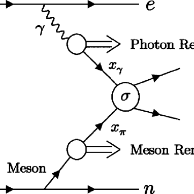
In high- jet photoproduction with , two types of processes contribute to the cross section, namely direct and resolved photon processes. In direct processes, the exchanged photon participates in the hard scattering as a point-like particle. In resolved processes, the photon acts as a source of partons, one of which interacts with a parton from the incoming hadron, see Fig. 1. The more complex structure of the resolved photon may increase the probability for the leading baryon to rescatter. This can cause the baryon to be scattered out of the detector acceptance, resulting in a depletion of detected baryons. Thus, fewer leading baryons (i.e. more rescatterings) are expected in resolved than in direct processes.
This effect was searched for, but not confirmed, in diffractive production of dijets in photoproduction [27, 28] and DIS [29, 27], where the leading proton has . However, a comparison of leading neutron rates in photoproduction and DIS showed a scale dependent suppression of neutrons [14, 17, 20]; the rates of neutrons were in good agreement with the expectations from rescattering models [23, 24].
This paper reports the observation of the photoproduction of dijets in association with a leading neutron:
| (3) |
where denotes the remainder of the final state. The number of events is almost an order of magnitude higher than used for previous results [14, 18]. Cross sections are presented as functions of the jet transverse energy, , jet pseudorapidity, , the fraction of the photon energy carried by the dijet system, , the photon-proton center-of-mass energy, , and the fraction of the proton four-momentum participating in the reaction, . In addition, the fraction of photoproduction events with a leading neutron as functions of these variables is shown as a test of vertex factorization. Finally, the and distributions of the leading neutrons are shown in dijet photoproduction and compared to similar results in DIS[20].
2 Experimental setup
The data sample used in this analysis was collected with the ZEUS detector at HERA and corresponds to an integrated luminosity of taken during the year 2000. During this period, HERA operated with protons of energy and positrons of energy , yielding a center-of-mass energy of .
A detailed description of the ZEUS detector can be found elsewhere [30]. A brief outline of the components most relevant for this analysis is given below. Charged particles were tracked in the central tracking detector (CTD) [31, *npps:b32:181, *nim:a338:254], which operated in a magnetic field of provided by a thin superconducting coil. The CTD consisted of 72 cylindrical drift chamber layers, organized in 9 superlayers covering the polar-angle111The ZEUS coordinate system is a right-handed Cartesian system, with the axis pointing in the proton beam direction, referred to as the “forward direction”, and the axis pointing towards the center of HERA. The coordinate origin is at the nominal interaction point. The pseudorapidity is defined as , where the polar angle, , is measured with respect to the proton beam direction. region . The transverse-momentum resolution for full-length tracks was , with in GeV.
The high-resolution uranium–scintillator calorimeter (CAL) [34, *nim:a309:101, *nim:a321:356, *nim:a336:23] consisted of three parts: the forward (FCAL), the barrel (BCAL) and the rear (RCAL) calorimeters. Each part was subdivided transversely into towers and longitudinally into one electromagnetic section (EMC) and either one (in RCAL) or two (in BCAL and FCAL) hadronic sections (HAC). The smallest subdivision of the calorimeter is called a cell. The CAL energy resolutions, as measured under test-beam conditions, are for electrons and for hadrons ( in GeV). The forward-plug calorimeter (FPC) [38] around the beam-pipe in the FCAL extended calorimetry to the region . It was a lead–scintillator calorimeter with a hadronic energy resolution of ( in GeV).
The forward neutron detectors are described in detail elsewhere [39, 20]; the main points are summarized briefly here. The forward neutron calorimeter (FNC) was installed in the HERA tunnel at and at m from the interaction point in the proton-beam direction. It was a lead–scintillator calorimeter, segmented vertically into towers to allow the separation of electromagnetic and hadronic showers by their energy sharing among towers. The energy resolution for neutrons, as measured in a beam test, was , with neutron energy in GeV. The energy scale of the FNC was determined with a systematic uncertainty of . The forward neutron tracker (FNT) was installed in the FNC at a depth of one interaction length. It was a hodoscope designed to measure the position of neutron showers, with two planes of scintillator fingers used to reconstruct the and positions of showers. The position resolution was . Veto counters were used to reject events in which particles had interacted with the inactive material in front of the FNC. Magnet apertures limited the FNC acceptance to neutrons with production angles less than mrad, which corresponds to transverse momenta .
3 Data selection and kinematic variables
A three-level trigger system was used to select events online [30, 42]. At the second level, cuts were made to reject beam-gas interactions and cosmic rays. At the third level, jets were reconstructed using the energies and positions of the CAL cells. Events with at least two jets with transverse energy in excess of GeV and below were accepted. No requirement on the FNC was made at any trigger level.
Offline, tracking and calorimeter information were combined to form energy-flow objects (EFOs) [43, 44]. The center-of-mass energy, , was reconstructed using the Jacquet-Blondel method [45] as , where is an estimator of the inelasticity variable , and ; is the energy of EFO with polar angle . The sum runs over all EFOs. The energy was corrected for energy losses using the Monte Carlo (MC) samples described in Section 4. After corrections, the sample was restricted to GeV. Events with a reconstructed positron candidate in the main detector were rejected. The selected photoproduction sample consisted of events from interactions with GeV2 and a mean GeV2.
The cluster algorithm [46] was used in the longitudinally invariant inclusive mode [47] to reconstruct jets in the measured hadronic final state from the energy deposits in the CAL cells (calorimetric jets). The axis of the jet was defined according to the Snowmass convention [48]. The jet search was performed in the plane of the laboratory frame. Corrections [49] to the jet transverse energy, , were applied as a function of the jet pseudorapidity, , and , and averaged over the jet azimuthal angle. Events with at least two jets of , where is the transverse energy of the highest (second highest) jet, and , were retained.
Leading neutron events were selected from the dijet sample by applying criteria described previously [20]. The main requirements are listed here. Events were required to have energy deposits in the FNC with energy ( and timing consistent with the triggered event. In addition the deposits had to be close to the zero-degree point in order to reject protons bent into the FNC top section. Electromagnetic showers from photons were rejected by requiring the energy sharing among the towers to be consistent with a hadronic shower. Showers which started in dead material upstream of the FNC were rejected by requiring that the veto counter had a signal of less than one mip. Additional information from the FNT was used to select a subsample of events where a good position and thus measurement was possible. The channel with the largest pulse-height in each of the hodoscope planes was required to be above a threshold to select neutrons which showered in front of the FNT plane, and transverse shower profiles were required to have only one peak to minimize the influence of shower fluctuations.
After the requirements described above, the final dijet sample contained 583168 events, of which a subsample of 9193 events had a neutron tag, and 4623 of these also had a well measured neutron position.
The fractions of the photon and proton four-momenta entering the hard scattering, and respectively, were reconstructed via
| (4) |
| (5) |
where and are the pseudorapidity and transverse energy, respectively, of the highest (second highest) jet. The observable was used to separate the underlying photon processes since it is small (large) for resolved (direct) processes. The fraction of the exchanged pion four-momentum entering the hard scattering, in Fig. 1, was reconstructed as .
4 Monte Carlo simulations
4.1 Detector corrections
Samples of MC events were generated to study the response of the central detector to jets of hadrons and the response of the forward neutron detectors. The acceptances of the central and forward detectors are independent and the overall acceptance factorizes as the product of the two; they were evaluated using two separate MC programs.
The programs Pythia 6.221 [50] and Herwig 6.1 [51, *jhep:0101:010] were used to generate photoproduction events for resolved and direct processes producing dijets in the central detector. Fragmentation into hadrons was performed using the Lund string model [52] as implemented in Jetset [53, *cpc:135:238, 55, *cpc:43:367] in the case of Pythia, and a cluster model [57] in the case of Herwig. The generated events were passed through the Geant 3.13-based [58] ZEUS detector- and trigger-simulation programs [30]. They were reconstructed and analyzed by the same program chain as the data.
The Pythia program was used to determine the central-detector acceptance corrections. Samples of resolved and direct processes were generated separately. The resolved sample was reweighted as a function of and the direct sample as a function of . The reweighting and relative contributions of the two samples were adjusted to give the best description of the measured and distributions. Different reweighting and mixing factors were applied for the inclusive and neutron-tagged jet samples.
The Herwig program was used to check the systematic effects of the detector corrections. Direct and resolved photon processes were generated with default parameters and multiple interactions turned on.
A detailed description of the efficiencies and correction factors for the leading neutron measurements is given elsewhere [20].
4.2 Model comparisons
Previous studies have shown that MC models generating leading neutrons from the fragmentation of the proton remnant do not describe the neutron and distributions in DIS nor in photoproduction [20]. Models incorporating pion exchange gave the best description of the leading neutrons; also models with soft color interactions (SCI) [59] were superior to the fragmentation models. Monte Carlo programs incorporating these non-perturbative processes were used for comparison to the present dijet photoproduction data.
The Rapgap model incorporates pion exchange to simulate leading baryon production. It also includes Pomeron exchange to simulate diffractive events. These processes are mixed with standard fragmentation according to their respective cross sections. The PDF parameterizations used were CTEQ5L [60] for the proton, the GRV-G LO [61] for the photon, the H1 fit 5 [62] for the Pomeron and GRV-P LO fit [63] for the pion. The light-cone exponential flux factor [64] was used to model pion exchange.
The SCI model assumes that soft color exchanges give variations in the topology of the confining color-string fields which then hadronize into a final state which can include a leading neutron. It was interfaced to the Pythia program [65]; this implementation of Pythia did not include multiple parton interactions.
5 Systematic uncertainties
Systematic uncertainties associated with the CTD and the CAL influence the jet measurement; those associated with the FNC influence the neutron measurement. They are considered separately.
For the jet measurements, the systematic effects are grouped into the following classes, their contributions to the uncertainties on the cross sections being given in parentheses:
-
•
knowledge of absolute jet energy scale to 3%: (1–6%);
-
•
model dependence: the acceptances were estimated using Herwig instead of Pythia tuned as described in the previous section (5–9%);
-
•
event selection: variation of and cuts by one standard deviation of the resolution (1–6% each for and ).
Together, these effects resulted in uncertainties of 7–15% on the jet cross sections. The overall normalization has an additional uncertainty of 2.25% due to the uncertainty in the luminosity measurement.
An extensive discussion of the systematic effects related to the neutron measurement is given elsewhere [20]; the effects are summarized here. The neutron acceptance is affected by uncertainties in the beam zero-degree point and the dead material map, and uncertainties in the distributions which enter into the computation of the neutron acceptance. The 2% uncertainty on the FNC energy scale also affects the and distributions. Systematic uncertainties from these effects were typically 5–10% of the measured quantities, for example the exponential slopes. The systematic variations largely affect the neutron acceptance and result in a correlated shift of neutron yields. Corrections for efficiency of the cuts and backgrounds in the leading neutron sample were applied to the normalization of the neutron yields. The corrections accounted for veto counter over- and under-efficiency and neutrons from proton beam-gas interactions. The overall systematic uncertainty on the normalization of the neutron cross sections from these corrections was . Combined with the other neutron systematics, the overall systematic uncertainty on the total neutron rate was .
6 Results
6.1 Jet cross sections and ratios
The inclusive dijet and neutron-tagged dijet photoproduction cross sections have been measured for jets with and , in the kinematic region and , with the additional restriction of and mrad for the neutron-tagged sample. The fraction of dijet events with a leading neutron, the yield , in the measured kinematic region is
| (6) |
In this ratio, most of the systematic effects of the dijet selection cancel, and the uncertainty is dominated by the systematic effects of the neutron selection.
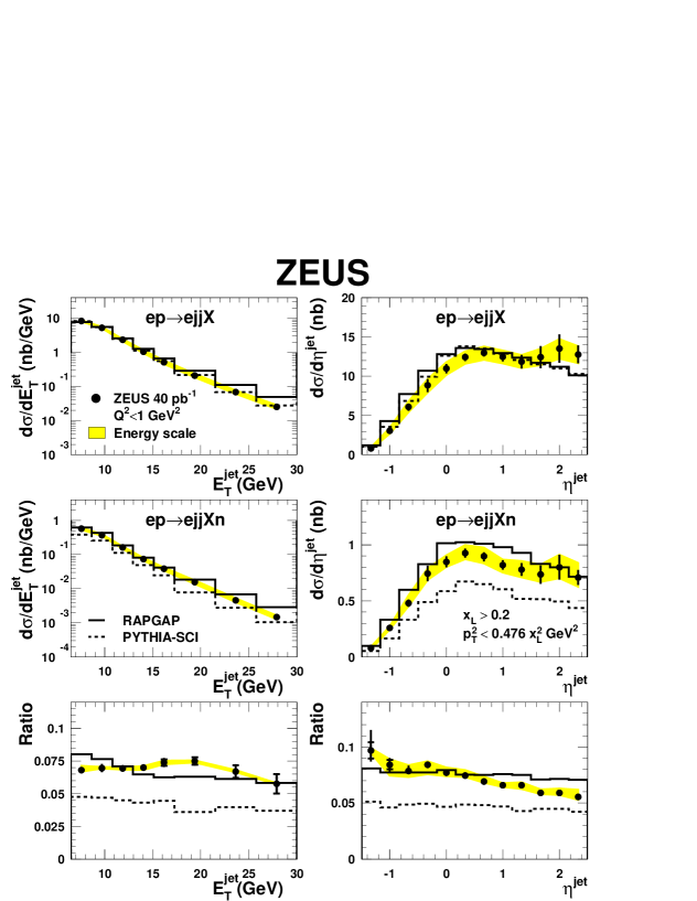
The differential cross sections for neutron-tagged and untagged events as functions of the jet variables and are presented in Fig. 2 and summarized in Table 1. They contain two entries per event, one for each jet. Also shown are the neutron yields as defined in Eq. (6) as a function of the relevant variable. The cross sections as functions of show a reduction of about three orders of magnitude within the measured range. The neutron yield is approximately constant as a function of . The cross sections as functions of rise over the range ; for higher values of they flatten. The neutron yield decreases with .
Figure 2 also shows the predictions of the Rapgap and SCI programs implemented as described in Section 4.2. Both are close in magnitude to the inclusive data. They both describe the steep drop with and the shape of the distributions. For neutron-tagged events Rapgap slightly overestimates and the SCI model clearly underestimates the cross section. They underestimate the decrease of the neutron yield with .
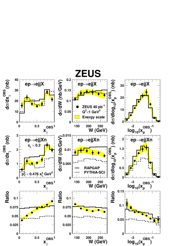
The differential cross sections as functions of the event variables , and are presented in Fig. 3 and summarized in Table 2. The cross sections as functions of show two peaks at and which can be attributed to the resolved- and direct-photon contributions, respectively. The neutron-tagged sample has a significantly smaller resolved contribution at low . This is seen clearly in the yield which rises by a factor of two from low to high . The cross sections are roughly flat as a function of ; the yield exhibits a mild decrease with increasing . The measured range of is 0.04 to 0.25 and the cross section peaks close to . The neutron yield decreases by a factor of two across the range measured.
Also shown in Fig. 3 are the predictions of the Rapgap and SCI models. Rapgap does not have a two-peaked structure as a function of , whereas the SCI model predicts the drop in cross section at central values of exhibited by the data. For the neutron-tagged sample, Rapgap overestimates the cross section in the resolved regime while SCI underestimates the cross section in the direct regime. Both models predict the relatively weak dependence of the cross section on and describe reasonably well the shape of the distribution. Neither model can reproduce the dependence of the neutron yield on and . The Rapgap model predicts a small decrease of the neutron yield with . However, the decrease is more pronounced in the data. The SCI model does not reproduce this feature at all.
The dependence of the neutron yield on , and as seen in Figs. 2 and 3 indicates a violation of vertex factorization. This might be explained by the Regge factorization as discussed in Section 1. The factorization violations seen in different variables are connected. A strong anticorrelation between the direct contribution and and is apparent in the data in Fig. 4. Events with low values of these variables contain up to 80% direct component, events with high values contain up to 90% resolved component. The observed drop of neutron yields at high and can thus be accounted for by a lower neutron yield in the resolved photon contribution. The smaller dependence of the neutron yield on and is consistent with this mechanism.
The H1 collaboration has also reported similar measurements [18]. They were made in a similar region of , and as the present analysis, but restricted to . The same pattern of vertex factorization violation was observed there. Also, after accounting for the different ranges, the cross sections are consistent.
6.2 Neutron distribution and pion structure
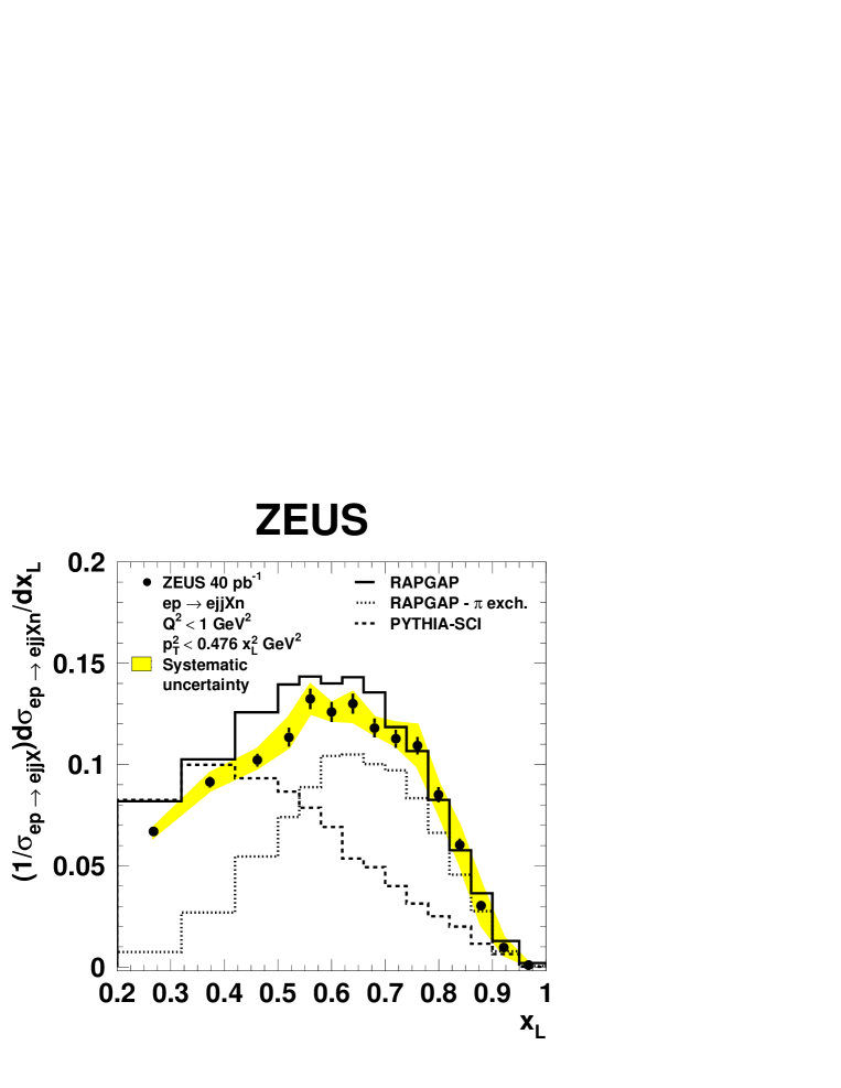
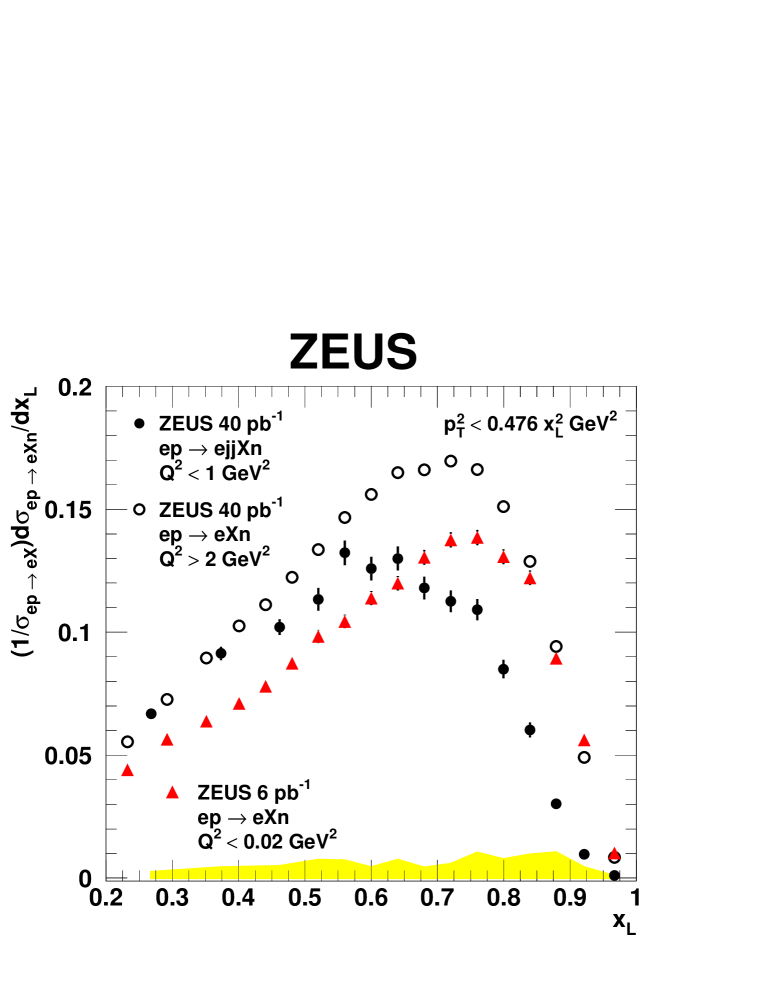
Figure 5 shows the normalized differential cross-section for neutrons with , which corresponds to . The distribution rises from the lowest values due to the increase in phase space. It reaches a maximum for , and falls to zero at the endpoint . Also shown are the predictions of the MC models. The Rapgap program gives a fair description of both the shape and normalization of the data, although its prediction is significantly above the data for . The SCI model does not describe the data, predicting too few events with neutrons and with a spectrum peaked at too low . Also shown in Fig. 5 is the pion-exchange contribution to the Rapgap prediction for the distribution. This contribution is essential for the Rapgap prediction to describe the measured distribution. It dominates for . Thus, in this region the dijet photoproduction data are sensitive to the pion structure.
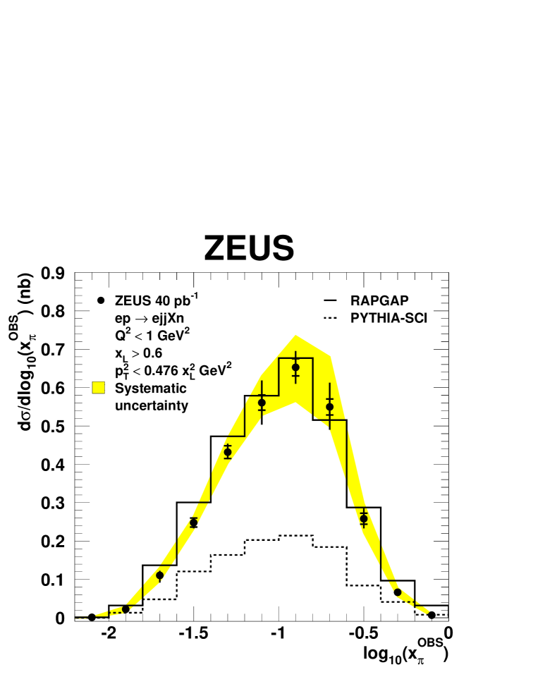
Figure 6 shows the neutron cross section as a function of for ; the values are listed in Table 3. The range in is from to ; the distribution peaks near . Also shown in Fig. 6 are the predictions of Rapgap and SCI. The former provides a good description of the data while the latter underestimates the cross section by about a factor of three. It should be noted that Rapgap, using the pion PDF parameterization GRV-P LO [63] based on fixed-target data with , is able to describe the cross section down to .
6.3 distributions
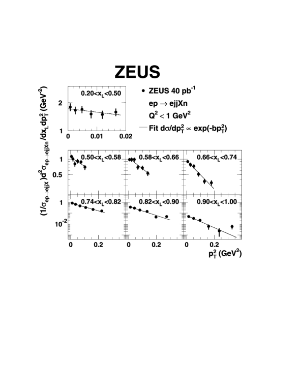
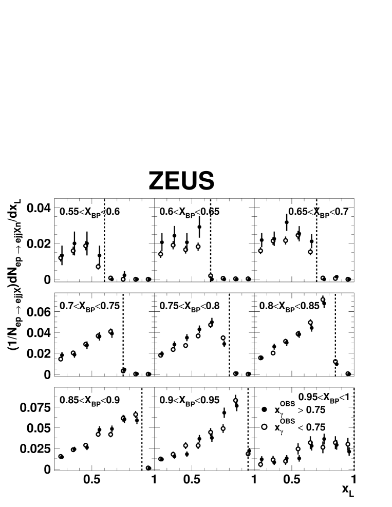
The distributions of the leading neutrons in different bins are shown in Fig. 7 and summarized in Table 4. They are presented as normalized doubly differential distributions, . The bins in are at least as large as the resolution, which is dominated by the spread of the proton beam. The varying ranges of the data are due to the aperture limitation. The line on each plot is a fit to the functional form . Each distribution is compatible with a single exponential within the statistical uncertainties. Thus, with the parameterization
| (7) |
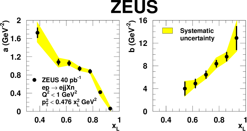
the neutron distribution is characterized by the slopes and intercepts . The results of exponential fits in bins of for the intercepts and the slopes are shown in Fig. 8 and summarized in Table 5. The systematic uncertainties were evaluated by making the variations discussed in Section 5 and repeating the fits. The intercepts fall rapidly from the lowest , drop mildly in the region , and fall to zero at the endpoint . In the lowest bin, the slope is consistent with zero and is not plotted; above the slope rises roughly linearly to a value of at .
6.4 Comparisons of different processes
6.4.1 Comparison to neutron production in DIS
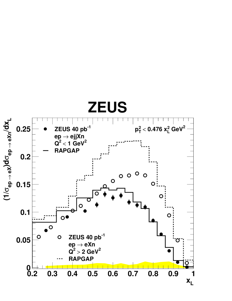
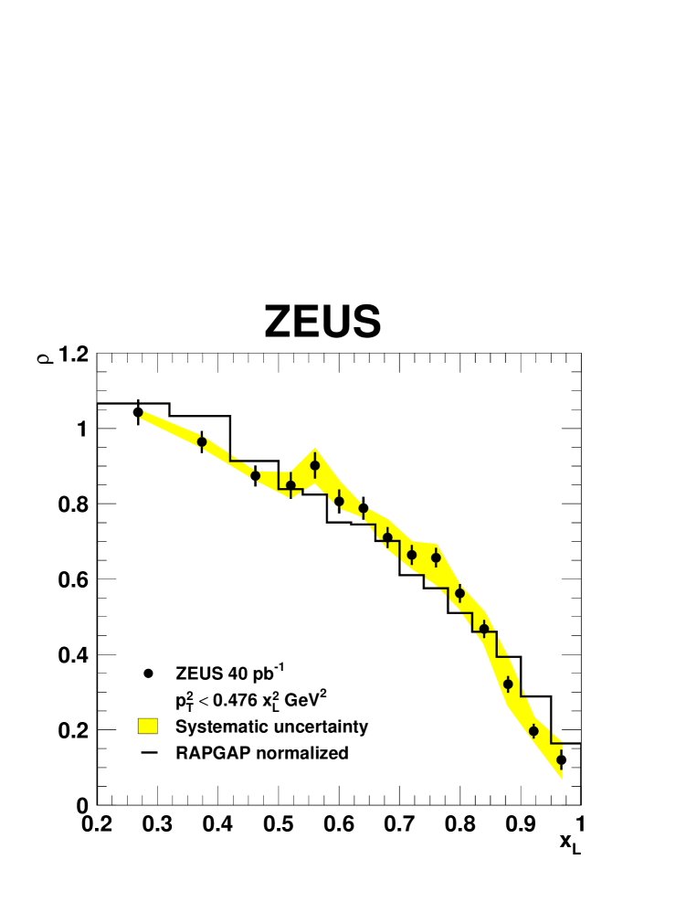
Figure 9 shows the normalized distribution of leading neutrons in dijet photoproduction and in inclusive DIS with [20]. The yield of neutrons from dijet photoproduction agrees with that in DIS at low , but is lower at higher . For the yield in dijet photoproduction is more than a factor of two lower than in inclusive DIS.
Figure 9 also shows the predictions of Rapgap for dijet photoproduction and DIS. The predicted shapes are in fair agreement with the measurements. However, the predicted neutron yield is too high for dijet photoproduction and too high for DIS. The shapes of the distributions for the two processes are compared using the ratio
| (8) |
The result is shown in Fig. 10. After normalizing each prediction to its respective data set, Rapgap provides a fair description of the drop of the neutron yield with in dijet photoproduction relative to that in DIS.
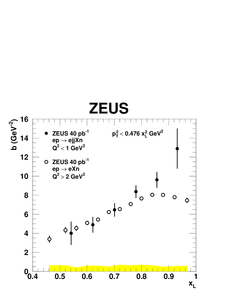
Figure 11 shows the exponential slopes for dijet photoproduction and inclusive DIS. They are similar in magnitude and both rise with . Although the slopes rise somewhat faster with in the dijet photoproduction data, there is no statistically significant difference between the two sets except for .
6.4.2 Comparison of dijet direct and resolved photon contributions
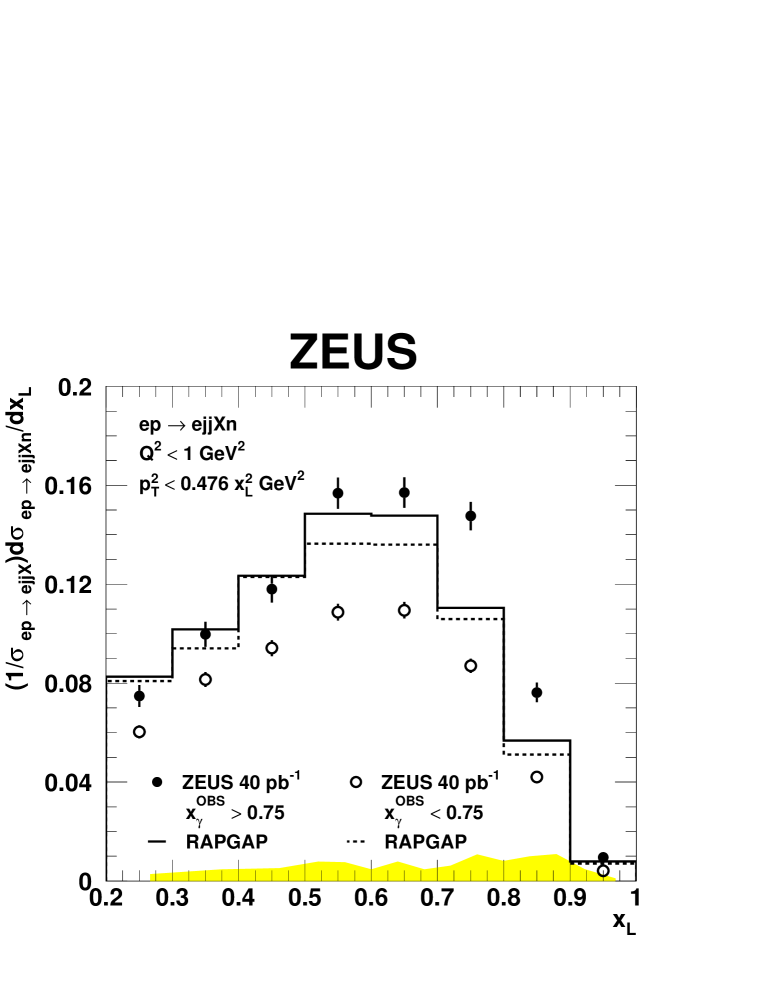
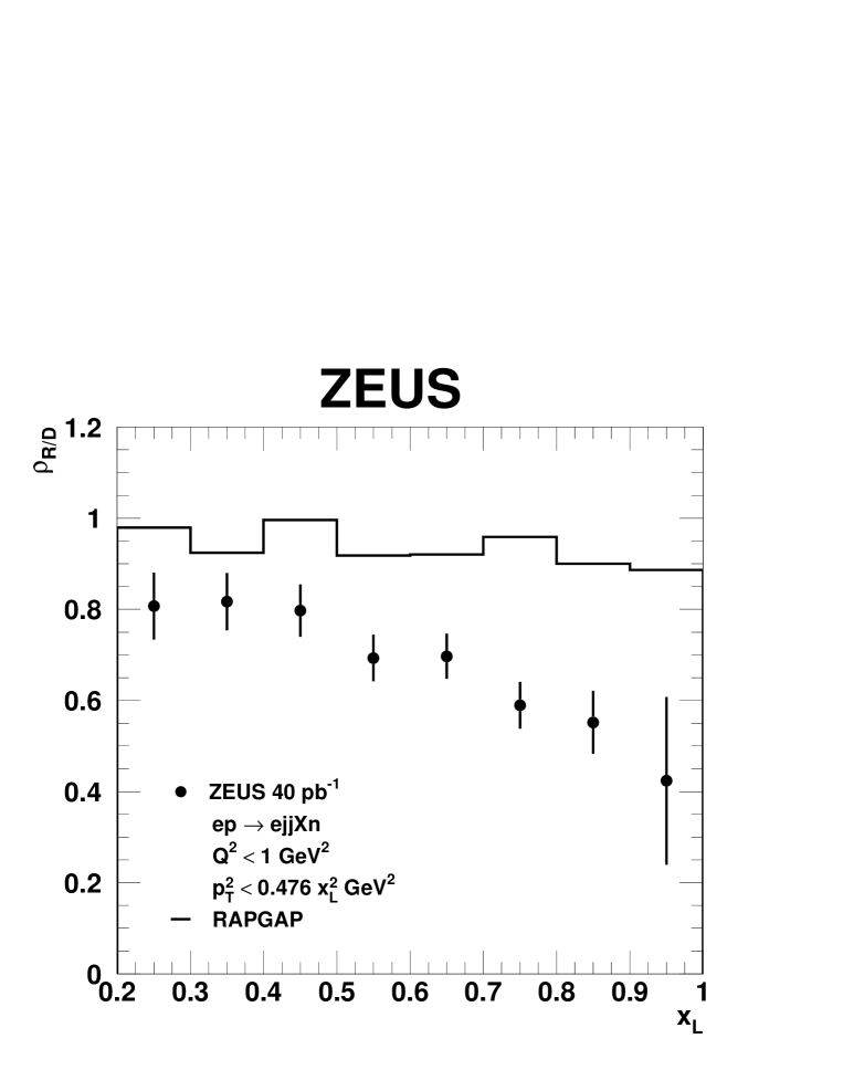
The neutron distributions in the dijet photoproduction data, enriched in direct and resolved processes, are shown in Fig. 12, normalized to their corresponding samples without a neutron requirement. In the resolved contribution, relatively fewer neutrons are observed. Figure 12 also shows the predictions of Rapgap for the distributions of the direct and resolved contributions. Figure 13 presents the ratio between the resolved and direct contributions to the cross section,
| (9) |
as a function of for data and the Rapgap prediction. The magnitude and shape are not described by Rapgap.
6.5 Role of kinematic constraints
The distributions for dijet photoproduction and for DIS are depicted in Fig. 9. It is interesting to investigate whether the difference between the two distributions is a characteristic of the transition or if it is a kinematic effect, due to different forward energy flows. To investigate such kinematic constraints, , the fraction of the proton beam energy going into the forward beampipe region, , was considered:
| (10) |
Here GeV is the proton beam energy and is the longitudinal energy-momentum, , with the sum running over all CAL and FPC cells with energy and polar angle . The energy of the leading neutron in an event is restricted to .
The distributions for dijet photoproduction and DIS, both without a leading neutron requirement, are shown in Fig. 14. The dijet photoproduction data are peaked at significantly lower and have a much larger tail at very low than the DIS data. Figure 15 shows the neutron distributions222 These distributions are not corrected for acceptance. The acceptance correction at a given depends only on the exponential slope . As shown in Fig. 11, the slopes for dijet photoproduction and DIS have very similar values. Differences in the acceptance correction are small and may be ignored for the comparisons made here. of the dijet photoproduction and DIS data in bins of , normalized by the number of events without a neutron requirement in the bin. They reflect the constraint . For any given value of , the two samples have nearly identical distributions, both in shape and normalization. This indicates that a given value of longitudinal energy-momentum measured in the central detector is associated with the same neutron yield and spectrum, regardless of whether the process is dijet photoproduction or DIS.
The effect of kinematic constraints from energy distributions in the central detector can also be investigated in the distributions of direct and resolved photoproduction as shown in Fig. 12. Figure 16 shows the distributions for the contributions from direct and resolved photons without a neutron tag being required. The resolved contribution peaks at lower and has a much larger tail at very low than the direct contribution. Figure 17 shows the neutron yield as a function of (not corrected for acceptance) in different bins of for the two contributions. As in the comparison to DIS, they verify the constraint , and for any given value of , the two samples have nearly identical distributions, both in shape and normalization. Thus the neutron spectra in dijet photoproduction as well as in DIS seem to depend only on the energy available in the proton-remnant region.
7 Discussion of rescattering
The good statistical accuracy of the data allows an investigation into effects of rescattering. The comparison of photoproduction to DIS offers one way to investigate rescattering effects, which are predicted to result in a lower neutron yield in photoproduction. Figure 18 shows the neutron yield as a function of for dijet photoproduction, inclusive DIS with , and inclusive photoproduction [20]. The inclusive photoproduction sample was obtained by tagging the scattered positron, with a resulting range of . The neutron yield for the positron-tagged inclusive sample agrees with the yield observed for inclusive DIS at high values of . At low , the neutron yield in inclusive photoproduction is smaller than in inclusive DIS. This was shown to be consistent with models of rescattering [23, 24, 25, 26]. The neutron yield is also smaller in dijet photoproduction, but the dependence of the suppression is reversed. The neutron yields are similar at low values of , whereas the neutron yield in dijet photoproduction is lower at high values. This was shown in Fig. 10.
The behavior of the neutron yield for dijet photoproduction is inconsistent with the rescattering models that described the yield for the positron-tagged photoproduction sample. Information concerning rescattering might be difficult to obtain from a direct comparison of dijet photoproduction and inclusive DIS data because of the different hadronic final states. A Regge factorization model without rescattering effects (Rapgap) can reproduce reasonably the differences in neutron yields between dijet photoproduction and inclusive DIS. A qualitative explanation can be deduced from Eq. (1): The cross section is proportional to , and this cross section rises steeply with for dijet production [49], whereas the cross section for the inclusive DIS reaction depends only weakly on [66, 67]. Therefore one expects a drop of the ratio of the dijet to DIS neutron yields as goes to 0. This is seen in Fig. 10.
Another way to look for such effects is to compare the direct and resolved contributions to dijet photoproduction. For the direct photon contribution, the photon is assumed to be pointlike; for the resolved photon interactions, the photon is assumed to have size and structure. This structure may be expected to increase the probability of rescattering. Indeed, the lower neutron yield in the resolved contribution to the cross section, as shown in the distribution in Fig. 3, seems to indicate such a loss mechanism. However, this seems in contradiction with the dependence of the effect, as shown in Figs. 12 and 13. These figures show that the neutron yield in the resolved contribution decreases relative to the yield in the direct contribution for increasing values of . This contradicts the predictions from the rescattering models which described the behavior of the inclusive photoproduction sample [20], where the effect goes in the opposite direction. Again, a comparison is complicated by the different hadronic final states in the direct and resolved contributions.
In summary, no clear conclusion on the presence of rescattering effects in dijet photoproduction can be drawn from the data alone. Only a comparison to a specific model could clarify this issue.
8 Summary
Differential cross sections for neutron-tagged and untagged dijet photoproduction, , have been measured. The measurements required jets with GeV, GeV and , in the kinematic region GeV2 and GeV, with the additional restriction of and mrad on the neutron-tagged sample. The cross sections were measured as functions of , , , and .
The ratios of the neutron-tagged to untagged differential cross sections show a reduction of the neutron yield at low , large , and large . These regions are dominated by resolved photon events.
The normalized leading-neutron distribution was measured. It is in reasonable agreement with the Rapgap MC model including pion exchange, which is essential to obtain a reasonable description of the data. In addition, the leading-neutron cross section as a function of , the fraction of the exchanged pion four-momentum entering the hard scattering, was measured in the restricted kinematic range , where pion exchange is the dominant production process, and good agreement with the model was found.
The leading-neutron cross sections as a function of in different regions of were measured in dijet photoproduction. The distributions are well described by exponentials, and the two-dimensional distribution is fully characterized by the slopes and intercepts from exponential fits in each bin.
The relation between the neutron yield and the fraction of the proton beam energy going into the forward beam pipe region, , was studied. The relative neutron rate as a function of seems to depend only on . This effect accounts for the observed differences between the distributions of the photoproduction dijet and the DIS data samples, and between those of the direct and resolved dijet samples.
No clear conclusion on the presence of rescattering effects can be drawn. While the reduction of the neutron yield in the region enriched in resolved photons is suggestive of the presence of a rescattering effect, the fact that this yield reduction is mainly at large seems to contradict the basic expectations of rescattering models.
Acknowledgments
We appreciate the contributions to the construction and maintenance of the ZEUS detector of many people who are not listed as authors. The HERA machine group and the DESY computing staff are especially acknowledged for their success in providing excellent operation of the collider and the data-analysis environment. We thank the DESY directorate for their strong support and encouragement, and are especially grateful for their financial support which made possible the construction and installation of the FNC. We are also happy to acknowledge the DESY accelerator group for allowing the installation of the FNC in close proximity to the HERA machine components.
10
References
- [1] J. Engler et al., Nucl. Phys. B 84, 70 (1975)
- [2] B. Robinson et al., Phys. Rev. Lett. 34, 1475 (1975)
- [3] W. Flauger and F. Mönnig, Nucl. Phys. B 109, 347 (1976)
- [4] J. Hanlon et al., Phys. Rev. Lett. 37, 967 (1976)
- [5] Y. Eisenberg et al., Nucl. Phys. B 135, 189 (1978)
- [6] V. Blobel et al., Nucl. Phys. B 135, 379 (1978)
- [7] H. Abramowicz et al., Nucl. Phys. B 166, 62 (1980)
- [8] J. D. Sullivan, Phys. Rev. D 5, 1732 (1972)
- [9] M. Bishari, Phys. Lett. B 38, 510 (1972)
- [10] S.N. Ganguli and D.P. Roy, Phys. Rep. 67, 201 (1980)
- [11] V. R. Zoller, Z. Phys. C 53, 443 (1992)
- [12] ZEUS Coll., M. Derrick et al., Phys. Lett. B 384, 388 (1996)
- [13] H1 Coll., C. Adloff et al., Eur. Phys. J. C 6, 587 (1999)
- [14] ZEUS Coll., J. Breitweg et al., Nucl. Phys. B 596, 3 (2001)
- [15] ZEUS Coll., S. Chekanov et al., Nucl. Phys. B 637, 3 (2002)
- [16] ZEUS Coll., S. Chekanov et al., Nucl. Phys. B 658, 3 (2003)
- [17] ZEUS Coll., S. Chekanov et al., Phys. Lett. B 590, 143 (2004)
- [18] H1 Coll., A. Aktas et al., Eur. Phys. J. C 41, 273 (2005)
- [19] ZEUS Coll., S. Chekanov et al., Phys. Lett. B 610, 199 (2005)
- [20] ZEUS Coll., S. Chekanov et al., Nucl. Phys. B 776, 1 (2007)
- [21] J. Benecke et al., Phys. Rev. 188, 2159 (1969)
- [22] T.T. Chou and C.N. Yang, Phys. Rev. D 50, 590 (1994)
- [23] N.N. Nikolaev, J. Speth and B.G. Zakharov, hep-ph/9708290 (1997)
- [24] U. D’Alesio and H.J. Pirner, Eur. Phys. J. A 7, 109 (2000)
- [25] A.B. Kaidalov et al., Eur. Phys. J. C 47, 385 (2006)
- [26] V.A. Khoze, A.D. Martin and M.G. Ryskin, Eur. Phys. J. C 48, 797 (2006)
- [27] H1 Coll., A. Aktas et al., Eur. Phys. J. C 51, 549 (2007)
- [28] ZEUS Coll., S. Chekanov et al., Eur. Phys. J. C 55, 177 (2008)
- [29] ZEUS Coll., S. Chekanov et al., Eur. Phys. J. C 52, 813 (2007)
- [30] ZEUS Coll., U. Holm (ed.), The ZEUS Detector. Status Report (unpublished), DESY (1993), available on http://www-zeus.desy.de/bluebook/bluebook.html
- [31] N. Harnew et al., Nucl. Inst. Meth. A 279, 290 (1989)
- [32] B. Foster et al., Nucl. Phys. Proc. Suppl. B 32, 181 (1993)
- [33] B. Foster et al., Nucl. Inst. Meth. A 338, 254 (1994)
- [34] M. Derrick et al., Nucl. Inst. Meth. A 309, 77 (1991)
- [35] A. Andresen et al., Nucl. Inst. Meth. A 309, 101 (1991)
- [36] A. Caldwell et al., Nucl. Inst. Meth. A 321, 356 (1992)
- [37] A. Bernstein et al., Nucl. Inst. Meth. A 336, 23 (1993)
- [38] A. Bamberger et al., Nucl. Inst. Meth. A 450, 235 (2000)
- [39] S. Bhadra et al., Nucl. Inst. Meth. A 394, 121 (1997)
- [40] J. Andruszków et al., Preprint DESY-92-066, DESY, 1992
- [41] J. Andruszków et al., Acta Phys. Pol. B 32, 2025 (2001)
- [42] W.H. Smith, K. Tokushuku and L.W. Wiggers, Proc. Computing in High-Energy Physics (CHEP), Annecy, France, Sept. 1992, C. Verkerk and W. Wojcik (eds.), p. 222. CERN, Geneva, Switzerland (1992). Also in preprint DESY 92-150B
- [43] ZEUS Coll., J. Breitweg et al., Eur. Phys. J. C 1, 81 (1998)
- [44] G.M. Briskin. Ph.D. Thesis, Tel Aviv University, Report DESY-THESIS 1998-036, 1998
- [45] F. Jacquet and A. Blondel, Proceedings of the Study for an Facility for Europe, U. Amaldi (ed.), p. 391. Hamburg, Germany (1979). Also in preprint DESY 79/48
- [46] S.Catani et al., Nucl. Phys. B 406, 187 (1993)
- [47] S.D. Ellis and D.E. Soper, Phys. Rev. D 48, 3160 (1993)
- [48] J.E. Huth et al., Research Directions for the Decade. Proceedings of Summer Study on High Energy Physics, 1990, E.L. Berger (ed.), p. 134. World Scientific (1992). Also in preprint FERMILAB-CONF-90-249-E
- [49] ZEUS Coll., S. Chekanov et al., Phys. Lett. B 560, 7 (2003)
- [50] T. Sjöstrand et al., Comp. Phys. Comm. 135, 238 (2001)
- [51] G. Marchesini et al., Comp. Phys. Comm. 67, 465 (1992)
- [52] B. Andersson et al., Phys. Rep. 97, 31 (1983)
- [53] T. Sjöstrand, Comp. Phys. Comm. 82, 74 (1994)
- [54] T. Sjöstrand et al., Comp. Phys. Comm. 135, 238 (2001)
- [55] T. Sjöstrand, Comp. Phys. Comm. 39, 347 (1986)
- [56] T. Sjöstrand and M. Bengtsson, Comp. Phys. Comm. 43, 367 (1987)
- [57] B.R. Webber, Nucl. Phys. B 238, 492 (1984)
- [58] R. Brun et al., geant3, Technical Report CERN-DD/EE/84-1, CERN, 1987
- [59] A. Edin, G. Ingelman and J. Rathsman, Phys. Lett. B 366, 371 (1996)
- [60] CTEQ Coll., H.L. Lai et al., Eur. Phys. J. C 12, 375 (2000)
- [61] M. Glück, E. Reya, and A. Vogt, Phys. Rev. D 45, 3986 (1992)
- [62] H1 Coll., C. Adloff et al., Z. Phys. C 76, 613 (1997)
- [63] M. Glück, E. Reya, and A. Vogt, Z. Phys. C 53, 651 (1992)
- [64] H. Holtmann et al., Phys. Lett. B 338, 363 (1994)
- [65] R. Enberg, G. Ingelman and N. Timneanu, Eur. Phys. J. C 33, 542 (2004)
- [66] ZEUS Coll., J. Breitweg et al., Eur. Phys. J. C 7, 609 (1999)
- [67] ZEUS Coll., S. Chekanov et al., Nucl. Phys. B 713, 3 (2005)
| (GeV) | (nb/GeV) | (nb/GeV) | (%) |
|---|---|---|---|
| 11.9 | |||
| 14.0 | |||
| 16.2 | |||
| 19.4 | |||
| 23.6 | |||
| 27.9 |
| (nb) | (nb) | (%) | |
|---|---|---|---|
| (nb) | (nb) | (%) | |
|---|---|---|---|
| 0.07 | |||
| 0.21 | |||
| 0.36 | |||
| 0.50 | |||
| 0.64 | |||
| 0.79 | |||
| 0.93 |
| (GeV) | (nb/GeV) | (nb/GeV) | (%) |
|---|---|---|---|
| 142 | |||
| 167 | |||
| 192 | |||
| 217 | |||
| 242 | |||
| 267 |
| (nb) | (nb) | (%) | |
|---|---|---|---|
| range | |||
|---|---|---|---|
| 0.20-0.50 | 0.38 | 7.74 | 1.797 0.169 |
| 2.52 | 1.659 0.156 | ||
| 4.86 | 1.699 0.155 | ||
| 7.97 | 1.511 0.151 | ||
| 1.18 | 1.492 0.149 | ||
| 1.65 | 1.585 0.149 | ||
| 0.50-0.58 | 0.54 | 4.84 | 1.135 0.092 |
| 1.58 | 1.008 0.107 | ||
| 3.03 | 0.808 0.095 | ||
| 4.97 | 0.915 0.093 | ||
| 7.40 | 0.884 0.086 | ||
| 1.03 | 0.694 0.078 | ||
| 0.58-0.66 | 0.62 | 6.50 | 0.982 0.073 |
| 2.12 | 0.985 0.091 | ||
| 4.08 | 0.984 0.089 | ||
| 6.68 | 0.694 0.070 | ||
| 9.94 | 0.678 0.064 | ||
| 1.39 | 0.526 0.058 | ||
| 0.66-0.74 | 0.70 | 8.39 | 0.896 0.061 |
| 2.74 | 0.781 0.071 | ||
| 5.27 | 0.726 0.067 | ||
| 8.64 | 0.507 0.051 | ||
| 1.29 | 0.366 0.041 | ||
| 1.79 | 0.343 0.041 | ||
| 0.74-0.82 | 0.78 | 1.05 | 0.840 0.053 |
| 3.43 | 0.664 0.058 | ||
| 6.60 | 0.462 0.047 | ||
| 1.08 | 0.330 0.036 | ||
| 1.61 | 0.223 0.028 | ||
| 2.24 | 0.162 0.024 | ||
| 0.82-0.90 | 0.86 | 1.28 | 0.364 0.032 |
| 4.20 | 0.289 0.035 | ||
| 8.08 | 0.194 0.027 | ||
| 1.33 | 0.145 0.021 | ||
| 1.97 | 0.044 0.011 | ||
| 2.75 | 0.048 0.011 | ||
| 0.90-1.00 | 0.93 | 1.52 | 0.049 0.009 |
| 5.03 | 0.033 0.009 | ||
| 9.68 | 0.022 0.007 | ||
| 1.59 | 0.006 0.003 | ||
| 2.36 | 0.002 0.002 | ||
| 3.29 | 0.006 0.003 |
| range | |||
|---|---|---|---|
| 0.20–0.50 | 0.38 | ||
| 0.50–0.58 | 0.54 | ||
| 0.58–0.66 | 0.62 | ||
| 0.66–0.74 | 0.70 | ||
| 0.74–0.82 | 0.78 | ||
| 0.82–0.90 | 0.86 | ||
| 0.90–1.00 | 0.93 |