Note on galaxy catalogues in UHECR flux modelling

Abstract

We consider the dependence of ultra-high energy cosmic ray (UHECR) flux predictions on the choice of galaxy catalogue. We demonstrate that model predictions by Koers & Tinyakov (2009b), based on the so-called KKKST catalogue, are in good agreement with predictions based on the XSCz catalogue, a recently compiled catalogue that contains spectroscopic redshifts for a large fraction of galaxies. This agreement refutes the claim by Kashti (2009) that the KKKST catalogue is not suited for studies of UHECR anisotropy due to its dependence on photometric redshift estimates. In order to quantify the effect of galaxy catalogues on flux predictions, we develop a measure of anisotropies associated with model flux maps. This measure offers a general criterion to study the effect of model parameters and assumptions on the predicted strength of UHECR anisotropies.

1 Introduction

Galaxy catalogues are an indispensable tool to model the structure of the local Universe, as required for studies of ultra-high energy cosmic ray (UHECR) anisotropy. Many such studies (e.g. Cuoco et al. 2006; Kashti & Waxman 2008; Takami et al. 2009; Kashti 2009) have used the PSCz catalogue (Saunders et al., 2000) for this purpose. This catalogue, however, has its drawbacks: it suffers from incomplete sky coverage, it may underestimate galaxy counts in high-density regions (Huchra et al., 2007), and it has limited statistics. The 2MASS galaxy catalogue (Jarrett et al., 2000; Jarrett, 2004; Skrutskie, M. F. et al., 2006), offering complete sky coverage (except for the galactic plane) and excellent statistics, improves on these issues. However, this catalogue does not contain spectroscopic redshifts so that redshifts have to be estimated by photometry, i.e. from the observed brightness under the assumption of a standard intrinsic brightness in a specific band. Efforts to obtain spectroscopic redshifts for 2MASS galaxies are ongoing. The resulting catalogue, termed XSCz, is presently being compiled.

Motivated by the imperfection of existing galaxy catalogues, Kalashev et al. (2008) have compiled a hybrid catalogue that contains galaxies with spectroscopic redshifts from the (HYPER)LEDA database (Paturel et al., 2003) within 30 Mpc and galaxies from the 2MASS Extended Source catalogue (Jarrett et al., 2000) at larger distances, for which photometric redshift estimates are used (the two contributions are of course normalized appropriately). This catalogue, which we have termed the KKKST catalogue, is used in Koers & Tinyakov (2009b; hereafter paper I)

The adequacy of the KKKST catalogue for UHECR flux modelling is questioned by Kashti (2009) because of its dependence on photometric redshift estimates. The errors in these estimates give rise to errors in flux estimates, which may distort model flux maps and may lead to inaccurate model predictions. The uncertainty in photometric redshift estimates is indeed fairly large: Jarrett (2004) quotes an error of $10\%-20\%$ for most normal galaxies in the 2MASS survey (Kashti (2009) claims a $\sim$$30\%$ systematic uncertainty). In paper I, we deemed these uncertainties acceptable for two reasons. First, large-scale anisotropies in flux maps arise as a collective effect of many sources. Adding flux contributions of many individual galaxies reduces the relative strength of fluctuations (for the KKKST catalogue with a smearing angle of $\theta_{\rm s}=6^{\circ}$, as adopted in paper I, a model flux is composed of individual contributions of $\sim$$600$ galaxies). Second, the remaining uncertainties only affect the model flux beyond 30 Mpc, while the imprint of local structure is strongest at close distances.

In this paper we compare model fluxes based on the KKKST catalogue to model fluxes based on a preliminary version of the XSCz catalogue. This allows us to determine to which extent the flux predictions in paper I are contaminated by the inaccuracies in the catalogue used. The XSCz catalogue is very well suited to model the matter distribution in the Universe because of its completeness, large statistics, and spectroscopic redshift measurements. We therefore consider the resulting model fluxes as a benchmark against which UHECR flux predictions derived with the KKKST catalogue (as well as with the PSCz catalogue) can be cross checked. As we will demonstrate, flux predictions based on the KKKST catalogue (as well as on the PSCz) are in good agreement with the XSCz prediction. This provides an a posteriori verification of the accuracy of our models in paper I.

We also investigate, in a general setup, the relationship between galaxy catalogues and the predicted strength of UHECR anisotropies. For this purpose we develop a measure that quantifies the relation between model flux maps, which represent the model predictions for a given galaxy catalogue, and the test statistic $D$ (introduced in paper I), which is a measure of the strength of UHECR anisotropies. This measure can be used to assess the predicted strength of anisotropies from the “contrast” that is exhibited in model flux maps and is independent of event number. Because of its generality, this measure may also be useful to study the effect of other model parameters and assumptions (e.g., threshold energy, deflection angle, or injection spectrum) on the predicted strength of UHECR anisotropies.

This paper is organized as follows. In section 2 we compare model predictions from the KKKST and PSCz catalogues to predictions based on the XSCz catalogue. Section 3 concerns the relationship between galaxy catalogues and the predicted strength of UHECR anisotropies. We summarize our findings in section 4.

2 Accuracy of model flux maps

Figure 1: Distribution of the relative difference $\delta z/z$ between photometric and spectroscopic redshift estimates for individual galaxies in the XSCz catalogue. Inset: cumulative distribution of $|\delta z/z|$. In producing this figure we only used galaxies with $D>5$ Mpc.

We begin our analysis by considering the accuracy of photometric redshift determinations in the 2MASS catalogue. We compute the relative difference $\delta z/z:=(z_{\rm photo}-z_{\rm spec})/z_{\rm spec}$, where $z_{\rm photo}$ denotes a photometric redshift estimate and $z_{\rm spec}$ denotes a spectroscopic redshift, for all galaxies in the XSCz catalogue that have spectroscopic redshifts. Here, and throughout the paper, we only consider galaxies with $K_{s}$-magnitude below 12.50 in the XSCz catalogue. Spectroscopic redshifts are available for $\sim$70% of these relatively bright galaxies. The distribution of $\delta z/z$ is shown in Fig. 1. The inaccuracy in photometric redshift estimates is indeed fairly large: we find that the average value of $|\delta z/z|$, the absolute relative difference in redshift determinations, is 0.36.

Figure 2: Distribution of $\Delta f$ for individual galaxies in the XSCz catalogue. In producing this plot, we approximated fluxes as $\phi\propto D^{-2}$ and we only considered galaxies with $D>5$ Mpc.

The UHECR luminosity at the source being unknown, model flux predictions are conveniently formulated in terms of the normalized flux

$$f=\frac{\phi}{\langle\phi\rangle}\,,$$ (1)

where $\phi$ denotes a single-source flux and $\langle\phi\rangle$ is the average flux of all galaxies. (Note that the overall flux normalization is determined by observations). To get a rough estimate of the inaccuracies in flux predictions at the level of individual sources, we approximate the flux associated with every galaxy as $\phi\propto D^{-2}$, $D$ being the source distance (we take $D\propto z$ here). Here, and throughout this paper, we assume all sources have the same intrinsic luminosity. We then compute the quantity $\Delta f=f_{\rm photo}-f_{\rm spec}$, where $f_{\rm photo}$ is the normalized flux estimate based on the photometric redshift estimate and $f_{\rm spec}$ is the normalized flux derived from the spectroscopic redshift. The distribution of $\Delta f$ is shown in Fig. 2.

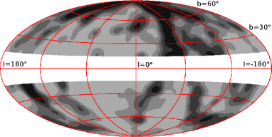
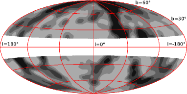
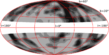
Figure 3: UHECR model flux maps for $E_{0}=60$ EeV, $\theta_{\rm s}=6^{\circ}$, and uniform exposure. The three panels show model predictions based on different galaxy catalogues: the KKKST catalogue (top panel), the XSCz catalogue (middle) and the PSCz catalogue (bottom). The gray bands are chosen such that each contains 1/5 of the model flux, with darker gray indicating larger flux.

We now consider model UHECR flux maps, which are generated using the methods described in paper I. Throughout this work we assume a proton composition and a power-law injection spectrum with spectral index $p=2.2$ extending to very high energies. We adopt a $\Lambda$CDM concordance model with Hubble constant $72$ km s^-1 Mpc^-1, and cosmological density parameters $\Omega_{m}=0.27$ and $\Omega_{\Lambda}=0.73$. Following the setup in paper I, we adopt a smearing angle $\theta_{\rm s}=6^{\circ}$. Using the method described in Koers & Tinyakov (2009a), we have verified that all catalogues contain sufficient galaxies to provide a good statistical description on this angular scale. We remove the region $|b|<15^{\circ}$ from our analysis because of incompleteness near the galactic plane. (We choose the same region for every catalogue for comparison; for the XSCz skymap this choice is overly conservative). Fig. 3 shows the flux maps for a threshold energy $E_{0}=60$ EeV. In Fig. 4 we show the distribution of flux differences $\Delta f=f_{\rm alt}-f_{\rm XSCz}$, where $f=\phi/\langle\phi\rangle$ denotes the normalized flux and the subscript refers to the catalogue that was used in the modelling (“alt” standing for either KKKST or PSCz). Here $\phi$ represents the integral UHECR flux in a given direction (as represented in Fig. 3) and $\langle\phi\rangle$ is the average flux on the sphere.

Figures 3 and 4 demonstrate that model predictions based on both the KKKST and PSCz catalogues are in good agreement with those from the XSCz catalogue. The average value of $|\Delta f|$ is 0.17 for the KKKST catalogue and 0.19 for the PSCz. At lower threshold energies the differences become smaller, while at higher energies they are somewhat larger. At $E_{0}=100$ EeV, for example, the average $|\Delta f|$ is 0.39 for the KKKST catalogue and 0.32 for the PSCz.

Sampling a flux map uniformly over the sky, one obtains a flux distribution associated with the map. This distribution encodes the relevant intrinsic properties of the flux map, i.e. properties relating to the strength of over- and underdense regions but not to their position on the sky. Postponing a more thorough discussion of the flux distribution to the next section, we point out here that the flux distribution corresponding to the KKKST flux map is broader than the flux distribution obtained with the PSCz catalogue (the XSCz is in between). This is reflected in the fact that the band of highest flux (darkest gray) in Fig. 3 occupies the smallest area on the sphere: 7.5% compared to 8.2% for the XSCz flux map and 10.4% for the PSCz flux map. For an isotropic flux map this number would be $1/5=20$%. We see that the KKKST map deviates most strongly from an isotropic flux map. As a consequence, model predictions based on this catalogue will exhibit the strongest departures from isotropy. We will use the term “contrast” to refer to the width of the flux distribution, strong contrast corresponding to a wide flux distribution and a strong deviation from isotropy.

How does the choice of galaxy catalogue affect the statistical tests proposed in paper I? We consider here the $D$-test, to which we will refer as the “flux sampling method”. The test defines a test statistic $D$ as the Kolmogorov-Smirnov (KS) distance $D_{\rm KS}$ between the cumulative distribution of flux values sampled by a set of UHECR events and a reference distribution that corresponds to the model that is tested (see paper I for details and discussion). Here and in the following we consider two models: the “Isotropy” model (denoted $\mathbf{I}$), which states that UHECR events are distributed isotropically (we do not consider experimental exposure here), and the “Structure” model (denoted $\mathbf{S}$), which states that UHECR sources trace the distribution of matter in the Universe. As a case study, we show in Fig. 5 the distribution of the test statistic $D$ for 20 UHECR events with energies in excess of 60 EeV. Here the reference distribution corresponds to an isotropic flux, so that the curve labeled “Isotropy” follows the universal KS self-correlation distribution (it is thus the same for all catalogues). The “Structure” distribution obtained from the PSCz catalogue is clearly closer to the “Isotropy” distribution than the “Structure” distribution obtained from the KKKST catalogue (the distribution from the XSCz being intermediary). This is reflected in the statistical power estimates: For a significance $\alpha=0.05$, we find $P=0.54$ for the KKKST catalogue, $P=0.46$ for the XSCz catalogue, and $P=0.37$ for the PSCz catalogue, where $P$ denotes the power to reject $\mathbf{I}$ when $\mathbf{S}$ is true. The difference in statistical powers can be related to the contrast in the model flux maps discussed in the previous paragraph. This relation will be explored in the next section.

We have recomputed power estimates and $p$-values for the $D$-test reported in paper I with the XSCz catalogue instead of the KKKST catalogue. At energies below 60 EeV we find that the power estimates change by only a few percent. At 100 EeV the XSCz catalogue leads to power estimates smaller by $\sim$20%, which is still acceptable in the light of other uncertainties. For the data obtained by the Pierre Auger Observatory and the AGASA experiment, we find no significant difference in $p$-values for the different catalogues.

Figure 4: Distribution of $\Delta f$ for the model fluxes shown in Fig. 3.

Figure 5: Distribution of test statistic $D$ for an isotropic reference distribution and test UHECR event sets following the distribution of matter as modelled from different catalogues. This figure applies to 20 events with threshold energy 60 EeV, and the distributions are obtained by sampling over $10^{4}$ independent Monte Carlo realizations.

3 Galaxy catalogues and predicted strength of anisotropies

In this section we investigate how the choice of catalogue affects the predicted strength of large-scale UHECR anisotropies. In order to quantify this strength we use the flux sampling test to measure deviations from isotropy. Although other tests will measure anisotropies in a different manner, a galaxy catalogue that yields a value for the $D$ test statistic close to the isotropic prediction will in general also yield outcomes close to the isotropic prediction in other tests (and similarly for predictions far away from the isotropic one).

The outcome of the flux sampling test depends on the number of events as well as on the distribution of model fluxes over the sky, i.e. the flux map. The first parameter is obviously independent of the choice of galaxy catalogue. All intrinsic properties of a galaxy catalogue that may affect the strength of anisotropies are contained in the flux map. Here and in the following, the expression “flux map” is used to refer to the flux map derived under $\mathbf{S}$ (i.e., assuming UHECR sources trace the distribution of matter in the Universe). The flux map also depends on threshold energy, UHECR injection spectrum, and average deflection angle.

Figure 6: The cumulative distribution $\mathcal{C}_{\rm iso}(f)$ for the KKKST, PSCz, and XSCz catalogues. This figure applies to threshold energy $E_{0}=60$ EeV and smearing angle $\theta_{\rm s}=6^{\circ}$.

The connection between flux maps and the strength of UHECR anisotropies can be illustrated by two limiting cases. First, consider the case that $\mathbf{S}$ would predict a uniform flux, so that the flux distribution would be a delta-function (minimal contrast). In that case UHECR events sample the sky uniformly under both $\mathbf{S}$ and $\mathbf{I}$ and model predictions become identical. In the opposite case of a very wide flux distribution (strong contrast), events will have a strong tendency to cluster in high-flux regions under $\mathbf{S}$, exhibiting strong anisotropy. The connection between flux distributions and the strength of anisotropies can be made explicit using the $D$-test. As shown in appendix A, under $\mathbf{S}$ the test statistic $D$ approaches the following limiting value as the number of events goes to infinity (recall that it approaches 0 in the same limit under $\mathbf{I}$):

$$D\to\int_{0}^{1}df\,\mathcal{C}_{\rm iso}(f)\,,$$ (2)

where $\mathcal{C}_{\rm iso}(f)$ denotes the normalized cumulative flux distribution under $\mathbf{S}$ and we recall that $f=\phi/\langle\phi\rangle$, $\phi$ being the integral UHECR flux and $\langle\phi\rangle$ the average value on the sphere. Equation (2) identifies the intrinsic property of a flux map that is important in determining the strength of UHECR anisotropies. It gives a precise meaning to the concept of “contrast” that was introduced in the previous section. It is related to the width of the flux distribution: A narrow flux distribution corresponds to a steeply rising cumulative distribution and, via equation (2), a value of $D$ close to 0.

Figure 7: Asymptotic value of $D$ for $N_{\rm ev}\to\infty$ for the KKKST, XSCz, and PSCz catalogues as a function of $E_{0}$.

The distribution $\mathcal{C}_{\rm iso}$ is shown in Fig. 6 for the three flux maps presented in Fig. 3. Comparing the surfaces under the curves for $0<f<1$, it is clear that the PSCz catalogue yields the smallest asymptotic value of $D$, and the KKKST catalogue the largest. The larger contrast in the KKKST catalogue implies stronger signatures of anisotropy. This explains the ordering of statistical powers that was found in the previous section.

In Fig. 7 we show the asymptotic value of $D$ from eq. (2) for different catalogues and threshold energies. We observe that the KKKST catalogue systematically predicts somewhat stronger anisotropies compared to the PSCz catalogue, in keeping with the results presented above and with the discussion in paper I. The XSCz prediction lies in between. For threshold energies $E_{0}\lesssim 60$ EeV, the XSCz curve is virtually identical to the KKKST one, while it approaches the PSCz curve at higher energies. The differences between the three curves are however small. In particular, they are smaller than the uncertainty induced by systematic errors in energy determination. (One may check that the curves corresponding to the KKKST and PSCz catalogues are within a 20% shift in energy applied to the XSCz prediction).

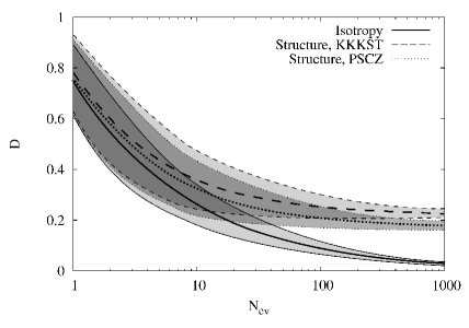
Figure 8: Average value of $D$ (thick lines) and 1-sigma contours (thin) as a function of event number $N_{\rm ev}$ for the KKKST and PSCz catalogues and for $E_{0}$ = 60 EeV. The full distribution for $N_{\rm ev}=20$ is shown in Fig. 5.

In reality the number of UHECR events is of course finite, and often not very large. The discriminatory power then depends not only on the flux map but also on event number. In this case, equation (2) provides a figure-of-merit that governs the asymptotic value of $D$. This is illustrated in Fig. 8, where we show the average value of $D$ and the 1-$\sigma$ bands as a function of event number. When $N_{\rm ev}$ becomes very large, $D$ approaches the asymptotic value computed with eq. (2): $0.22$ for the KKKST catalogue and $0.17$ for the PSCz catalogue.

4 Summary

In this paper we have investigated how the choice of galaxy catalogue affects UHECR model fluxes in a scenario where UHECR sources trace the distribution of matter in the Universe. The differences between the three catalogues considered here, the KKKST catalogue (Kalashev et al., 2008), the XSCz catalogue, and the PSCz catalogue (Saunders et al., 2000) are reasonably small. This is reassuring because all catalogues are supposed to be sampling the same underlying density field (barring biases induced by selection effects).

In section 2 we have shown that there is good agreement between model flux maps constructed with the KKKST and XSCz catalogues. The former was used by us earlier in paper I (Koers & Tinyakov, 2009b) The agreement is especially good at energies below 60 EeV, the regime where we have confronted models with experimental data in paper I. This comparison refutes the recent statement by Kashti (2009) that the KKKST catalogue is not suited for studies of UHECR anisotropy because of its dependence on photometric redshift estimates.

We have investigated the relation between the predicted strength of large-scale UHECR anisotropies and model flux maps from a general point of view in section 3. The intrinsic properties of an UHECR flux map, i.e. those properties relating to the strength of over- and underdense regions but not to their position on the sky, are contained in the flux distribution. Equation (2) demonstrates how this distribution can be used to determine the value of the $D$ test statistic in the limit of infinite events. This asymptotic value provides a measure of the expected anisotropy in UHECR arrival directions for sources tracing the distribution of matter in the Universe. We have compared these values for the KKKST, XSCz, and PSCz catalogues as a function of energy (see Fig. 7). The comparison shows that the KKKST catalogue typically yields stronger anisotropies than the PSCz catalogue, the XSCz catalogue being in between. The difference is however small in the light of the uncertainties induced by systematical errors in UHECR energy determination.

Appendix A Kolmogorov-Smirnov distance in the limit of infinite statistics

In this appendix we derive equation (2). We choose a general setup because the result is not limited to UHECR anisotropy tests, but is applicable to any experimental test that can be appropriately formulated.

Consider an experiment that records events which are characterized by a set of quantities $\vec{x}$ (these quantities may be observables or derived quantities). The space of all possible experimental results is denoted as $V$. Now consider two models, termed model $\mathbf{A}$ and model $\mathbf{B}$. Model $\mathbf{A}$ asserts that events sample $V$ uniformly, i.e. that the probability of registering quantities in the range $\vec{x}\ldots\vec{x}+d\vec{x}$ is independent of $\vec{x}$ (as long as $\vec{x}\in V$). Within model $\mathbf{B}$, on the other hand, the probability that an event has quantities in the range $\vec{x}\ldots\vec{x}+d\vec{x}$ is proportional to $f(\vec{x})d\vec{x}$, where $f$ is a non-trivial, known function. This function defines a map $\vec{x}\mapsto f$, which associates a real number $f$ to every event. Note that we leave the normalization of $f$ arbitrary.

Our aim is now to differentiate between models $\mathbf{A}$ and $\mathbf{B}$. We will do this by considering the distribution of $f$ over an observation, i.e. a series of registered events. We consider the limit of infinite statistics. The distribution of $f$ under model $\mathbf{A}$, denoted as $\mathcal{D}_{\mathbf{A}}(f)$, represents the distribution of $f$ over $V$. We assume this distribution is normalized, i.e.

$$\int_{0}^{\infty}df\mathcal{D}_{\mathbf{A}}(f)=1\,.$$ (3)

The distribution of $f$ under model $\mathbf{B}$ is denoted as $\mathcal{D}_{\mathbf{B}}(f)$. By construction,

$$\mathcal{D}_{\mathbf{B}}(f)=cf\mathcal{D}_{\mathbf{A}}(f)\,,$$ (4)

where

$$c=\left(\int_{0}^{\infty}dff\mathcal{D}_{\mathbf{A}}(f)\right)^{-1}$$ (5)

is a normalization constant to ensure that $\mathcal{D}_{\mathbf{B}}(f)$ is also normalized. Note that $1/c$ coincides with $\bar{f}_{\mathbf{A}}$, the average value of $f$ in model $\mathbf{A}$. We define cumulative distribution functions as

$$\mathcal{C}(f)=\int_{0}^{f}df^{\prime}\mathcal{D}(f^{\prime})\,.$$ (6)

The Kolmogorov-Smirnov distance $D_{\rm KS}$ is a measure of the difference between $\mathcal{C}_{\mathbf{A}}$ and $\mathcal{C}_{\mathbf{B}}$. As we will show, it can be expressed in terms of the cumulative distribution function $\mathcal{C}_{\mathbf{A}}(f)$ alone. First we recall that, by definition, $D_{\rm KS}=\max|D(f)|$, where $D(f)=\mathcal{C}_{\mathbf{A}}(f)-\mathcal{C}_{\mathbf{B}}(f)$ denotes the difference between the two cumulative distribution functions. This difference can be expressed as follows:

$$D(f)=\int_{0}^{f}df^{\prime}\mathcal{D}_{\mathbf{A}}(f^{\prime})\left(1-cf^{\prime}\right)\,.$$ (7)

Since $\mathcal{D}_{\mathbf{A}}$, $c$ and $f^{\prime}$ are strictly positive, the integral is maximal when $f=1/c=\bar{f}_{\mathbf{A}}$. Hence

$$D_{\rm KS}=D(\bar{f}_{\mathbf{A}})=\frac{1}{\bar{f}_{\mathbf{A}}}\int_{0}^{\bar{f}_{\mathbf{A}}}df^{\prime}\mathcal{C}_{\rm A}(f^{\prime})\,,$$ (8)

where the last equality has been obtained by integration by parts. Normalizing the function $f$ such that $\bar{f}_{\mathbf{A}}=1$, the r.h.s. of eq. (8) reduces to the integral of the cumulative distribution function $\mathcal{C}_{\mathbf{A}}$ up to $f=1$.

Two remarks are in order. First, equation (8) is a general result that is applicable to any statistical test for a model that can be formulated in terms of a probability function $f(\vec{x})$, where $\vec{x}$ is distributed uniformly in $V$ under the alternative model. The result applies to the UHECR anisotropy tests considered in this work by associating $\vec{x}=(l,\sin b)$, where $l$ and $b$ denote galactic coordinates, and $f=\phi/\langle\phi\rangle$, where $\phi$ denotes the model flux when UHECR sources trace the distribution of matter, and $\langle\phi\rangle$ is the average value on the sphere. Note that, by definition, $\bar{f}_{\mathbf{A}}=1$ in this case. Second, equation (8) determines $D_{\rm KS}$ in the limit of an infinite number of events. For finite event numbers, it is still a useful figure of merit because it determines the asymptotic behaviour (cf. Fig. 8).

References

- Cuoco et al. (2006) Cuoco A., Abrusco R. D., Longo G., Miele G., Serpico P. D., 2006, JCAP, 0601, 009
- Huchra et al. (2007) Huchra J., et al., 2007, The 2MASS Redshift Survey: http://www.cfa.harvard.edu/~huchra/2mass/ (version of Feb. 2007)
- Jarrett (2004) Jarrett T., 2004, arXiv: astro-ph/0405069
- Jarrett (2004) Jarrett T. H., 2004, Publications of the Astronomical Society of Australia, 21, 396
- Jarrett et al. (2000) Jarrett T. H., et al., 2000, AJ, 119, 2498
- Kalashev et al. (2008) Kalashev O. E., Khrenov B. A., Klimov P., Sharakin S., Troitsky S. V., 2008, JCAP, 0803, 003
- Kashti (2009) Kashti T., 2009, Nucl. Phys., A827, 570c
- Kashti & Waxman (2008) Kashti T., Waxman E., 2008, JCAP, 0805, 006
- Koers & Tinyakov (2009a) Koers H. B. J., Tinyakov P., 2009a, arXiv: 0907.0121 (accepted for publication in MNRAS)
- Koers & Tinyakov (2009b) Koers H. B. J., Tinyakov P., 2009b, JCAP, 0904, 003 (paper I)
- Paturel et al. (2003) Paturel G., Petit C., Prugniel P., Theureau G., Rousseau J., Brouty M., Dubois P., Cambrésy L., 2003, A&A, 412, 45
- Saunders et al. (2000) Saunders W., et al., 2000, MNRAS, 317, 55
- Skrutskie, M. F. et al. (2006) Skrutskie, M. F. et al., 2006, AJ, 131, 1163
- Takami et al. (2009) Takami H., Nishimichi T., Yahata K., Sato K., 2009, JCAP, 0906, 031