Constructing the self-force

Abstract

I present an overview of the methods involved in the computation of the scalar, electromagnetic, and gravitational self-forces acting on a point particle moving in a curved spacetime. For simplicity, the focus here will be on the scalar self-force. The lecture follows closely my review article on this subject [E. Poisson, Living Rev. Relativity 7, (2004), http://www.livingreviews.org/lrr-2004-6]. I begin with a review of geometrical elements (Synge’s world function, the parallel propagator). Next I introduce useful coordinate systems (Fermi normal coordinates and retarded light-cone coordinates) in a neighborhood of the particle’s world line. I then present the wave equation for a scalar field in curved spacetime and the equations of motion for a particle endowed with a scalar charge. The wave equation is solved by means of a Green’s function, and the self-force is constructed from the field gradient. Because the retarded field is singular on the world line, the self-force must involve a regularized version of the field gradient, and I describe how the regular piece of the self-field can be identified. In the penultimate section of the lecture I put the construction of the self-force on a sophisticated axiomatic basis, and in the concluding section I explain how one can do better by abandoning the dangerous fiction of a point particle.

1 Introduction

We consider a point particle moving on a world line $\gamma$ in a curved spacetime with metric $g_{\alpha\beta}$. The particle is either endowed with a scalar charge $q$ or an electric charge $e$, and we wish to calculate the effect of these charges on the motion of the particle. This motion is not geodesic, because the (scalar or electromagnetic) field created by the particle interacts with the particle and causes it to accelerate. In flat spacetime this effect is produced by a local distortion of the field lines associated with the particle’s acceleration. In curved spacetime there is no such local distortion when the particle moves freely; what happens instead is that the field interacts with the spacetime curvature and back-scatters toward the particle. As far as the particle is concerned, then, it interacts with an incoming wave, and the motion is not geodesic.

There is a gravitational analogue to these (scalar and electromagnetic) situations: Even in the absence of charges $q$ and $e$, we may wish to go beyond the test-mass description and consider the effect of the particle’s mass $m$ on its motion. There are two ways of describing this effect. We might say that the particle moves on a geodesic in a perturbed spacetime with metric $g_{\alpha\beta}+h_{\alpha\beta}$. Or we might say that the particle moves on an accelerated world line in the original spacetime with metric $g_{\alpha\beta}$. It is useful to keep both points of view active, and most researchers working in this field go freely back and forth between these modes of description. In the second view, the particle’s acceleration is associated with the perturbation $h_{\alpha\beta}$, which produces a gravitational self-force acting on the particle.

The scalar, electromagnetic, and gravitational self-force problems share many physical and mathematical features. In each case a moving charge is accompanied by a field: $q$ produces a scalar field $\Phi$, $e$ produces an electromagnetic field $A_{\alpha}$, and $m$ produces a gravitational perturbation $h_{\alpha\beta}$. In each case the field satisfies a linear wave equation in the background spacetime: $\Phi$ satisfies a scalar wave equation, $A_{\alpha}$ a vectorial equation derived from Maxwell’s equations, and $h_{\alpha\beta}$ a tensorial equation derived from the linearized Einstein equations. And in each case the self-force is equal to the gradient of the field evaluated on the particle’s world line.

This last observation reveals the problematic nature of this investigation. It is straightforward enough to calculate the scalar field $\Phi$, the vector potential $A_{\alpha}$, and the gravitational perturbation $h_{\alpha\beta}$ at a distance from the particle. But because the particle is pointlike, these quantities diverge on the world line, and derivatives of these quantities are even more singular. How is one supposed to deal with these singular expressions and extract from them the finite pieces that produce a well-defined effect, namely the self-force acting on the particle?

The purpose of this lecture is to offer some elements of answer to this question. My focus will be on the technical aspects of the problem, which I will try to describe without going overboard with derivations and mathematical precision. The preceding lecture by Bob Wald offers more on the conceptual aspects of the self-force, and other contributions describe ways of computing the self-force and its consequences. This lecture can be considered to be a light introduction to my massive review article published in Living Reviews in Relativity poisson:04b , to which I will frequently refer (as LRR); there the reader will find all the gory details of all the derivations omitted in the lecture.

For simplicity I will focus on the simplest exemplar of a self-force: the scalar self-force produced by a scalar field $\Phi$ on a scalar charge $q$. Understanding the details of this construction is a first step toward understanding the nature of the electromagnetic and gravitational self-forces; the computations involved are simpler, but the conceptual basis is essentially the same.

The self-force has a long history in theoretical physics, which is nicely summarized in a book by Herbert Spohn spohn:08 . The standard reference for the electromagnetic self-force in flat spacetime is Dirac’s famous 1938 paper dirac:38 . Dirac’s construction was generalized to curved spacetime in 1960 by DeWitt and Brehme dewitt-brehme:60 ; a technical error in their work was corrected by Hobbs hobbs:68 . The gravitational self-force was first computed in 1997 by Mino, Sasaki, and Tanaka mino-etal:97 ; a more direct derivation (based on an axiomatic approach) was later provided by Quinn and Wald quinn-wald:97 . Finally, the scalar self-force — the main topic of this lecture — was first constructed in 2000 by Ted Quinn quinn:00 .

2 Geometric elements

The construction of the self-force would be impossible without the introduction of geometric tools that were first fashioned by Synge synge:60 and independently by DeWitt and Brehme dewitt-brehme:60 . In this section I introduce the world function $\sigma(x,x^{\prime})$ and the parallel propagator $g^{\alpha}_{\ \alpha^{\prime}}(x,x^{\prime})$.

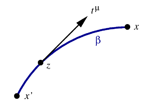
Figure 1: Geodesic segment $\beta$ between the spacetime points $x^{\prime}$ and $x$. The vector $t^{\mu}$ is tangent to this geodesic.

Let $x$ and $x^{\prime}$ be two points in spacetime, and let us assume that they are sufficiently close that there is a unique geodesic segment $\beta$ linking them. The segment is described by the parametric relations $z^{\mu}(\lambda)$, in which $\lambda$ is an affine parameter that runs from $0$ to $1$; we have that $z(0)=x^{\prime}$ and $z(1)=x$. The vector $t^{\mu}:=dz^{\mu}/d\lambda$ is tangent to $\beta$.

The world function is defined by

$$\sigma(x,x^{\prime}):=\frac{1}{2}\int_{0}^{1}g_{\mu\nu}(z)t^{\mu}t^{\nu}\,d\lambda.$$ (1)

It is numerically equal to half the squared geodesic distance between $x$ and $x^{\prime}$. When $\sigma<0$ the separation between $x$ and $x^{\prime}$ is timelike, and when $\sigma>0$ it is spacelike. The equation $\sigma(x,x^{\prime})=0$ describes the light cones of each point; if $x^{\prime}$ is kept fixed then $\sigma(x)=0$ describes the past and future light cones of $x^{\prime}$; if instead $x$ is kept fixed then $\sigma(x^{\prime})=0$ describes the past and future light cones of $x$.

The world function can be differentiated with respect to each argument. It can be shown (LRR Sec. 2.1.2) that

$$-\sigma^{\alpha^{\prime}}:=-\nabla^{\alpha^{\prime}}\sigma(x,x^{\prime})$$ (2)

is a vector at $x^{\prime}$ that is proportional to $t^{\mu}$ evaluated at that point. I use the convention that primed indices refer to the point $x^{\prime}$, while unprimed indices refer to $x$. It can also be shown that its length is given by

$$g_{\alpha^{\prime}\beta^{\prime}}\sigma^{\alpha^{\prime}}\sigma^{\beta^{\prime}}=2\sigma;$$ (3)

the length of $\sigma^{\alpha^{\prime}}$ therefore measures the geodesic distance between the two points. Because the vector points from $x^{\prime}$ to $x$, we have a covariant notion of a displacement vector between the two points.

The parallel propagator takes a vector $A^{\alpha^{\prime}}$ at $x^{\prime}$ and moves it to $x$ by parallel transport on the geodesic segment $\beta$. We express this operation as

$$A^{\alpha}(x)=g^{\alpha}_{\ \alpha^{\prime}}(x,x^{\prime})A^{\alpha^{\prime}}(x^{\prime}),$$ (4)

in which $A^{\alpha}$ is the resulting vector at $x$. The operation is easily generalized to dual vectors and other types of tensors (LRR Sec. 2.3).

The world function and the parallel propagator can be employed in the construction of a Taylor expansion of a tensor about a reference point $x^{\prime}$. Suppose that we have a tensor field $A^{\alpha\beta}(x)$ and that we wish to express it as an expansion in powers of the displacement away from $x^{\prime}$. The role of the deviation vector is played by $-\sigma^{\alpha^{\prime}}$, and the expansion coefficients will be ordinary tensors at $x^{\prime}$. We might write something like

$$A^{\alpha^{\prime}\beta^{\prime}}+A^{\alpha^{\prime}\beta^{\prime}}_{\ \ \ \ \gamma^{\prime}}(-\sigma^{\gamma^{\prime}})+\frac{1}{2}A^{\alpha^{\prime}\beta^{\prime}}_{\ \ \ \ \gamma^{\prime}\delta^{\prime}}(-\sigma^{\gamma^{\prime}})(-\sigma^{\delta^{\prime}})+\cdots,$$

but this defines a tensor at $x^{\prime}$, not $x$. To get a proper expression for $A^{\alpha\beta}(x)$ we must also involve the parallel propagator, and we write

$$A^{\alpha\beta}=g^{\alpha}_{\ \alpha^{\prime}}g^{\beta}_{\ \beta^{\prime}}\biggl{[}A^{\alpha^{\prime}\beta^{\prime}}-A^{\alpha^{\prime}\beta^{\prime}}_{\ \ \ \ \gamma^{\prime}}\sigma^{\gamma^{\prime}}+\frac{1}{2}A^{\alpha^{\prime}\beta^{\prime}}_{\ \ \ \ \gamma^{\prime}\delta^{\prime}}\sigma^{\gamma^{\prime}}\sigma^{\delta^{\prime}}+\cdots\biggr{]}.$$ (5)

Having postulated this form for the expansion, the expansion coefficients $A^{\alpha^{\prime}\beta^{\prime}}$, $A^{\alpha^{\prime}\beta^{\prime}}_{\ \ \ \ \gamma^{\prime}}$, and so on can be computed by repeatedly differentiating the tensor field and evaluating the results in the limit $x\to x^{\prime}$ (see LRR Sec. 2.4). For example, $A^{\alpha^{\prime}\beta^{\prime}}=\lim\,A^{\alpha\beta}$, as we might expect.

3 Coordinate systems

Self-force computations are best carried out using covariant methods. It is convenient, however, to display the results in a coordinate system that is well suited to the description of a neighbourhood of the world line $\gamma$. In this transcription it is advantageous to keep the coordinates in a close correspondence with the geometric objects (such as $\sigma^{\alpha^{\prime}}$) that appear in the covariant expressions. I find that two coordinate systems are particularly useful in this context: the Fermi normal coordinates $(t,x^{a}=s\omega^{a})$, and the retarded null-cone coordinates $(u,x^{a}=r\Omega^{a})$.

A third coordinate system, known as the Thorne-Hartle-Zhang coordinates thorne-hartle:85 ; zhang:86 , has also appeared in the self-force literature — they are the favoured choice of the Florida group led by Steve Detweiler and Bernard Whiting (see, for example, Ref. detweiler:05 ). The THZ coordinates are a variant of the Fermi coordinates, and they have some nice properties. But I find them less convenient to deal with than the Fermi or retarded coordinates, because they do not seem to possess a simple covariant definition. (The THZ coordinates may enjoy the mild Florida winters, but they are not robust enough to endure the tougher Canadian winters.) I shall not discuss the THZ coordinates here.

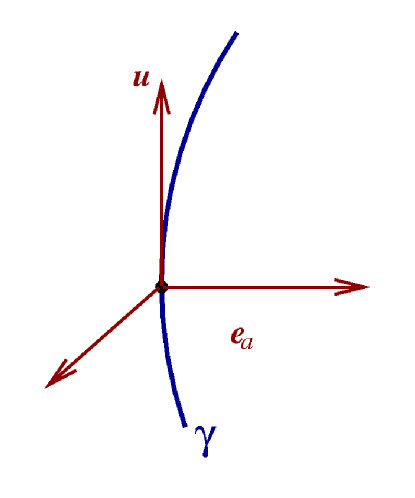
Figure 2: A tetrad of basis vectors on the world line $\gamma$. The unit timelike vector $u^{\mu}$ is tangent to the world line. The unit spatial vectors $e^{\mu}_{a}$ are mutually orthogonal and also orthogonal to $u^{\mu}$.

The Fermi and retarded coordinates share a basic geometrical construction on the world line. At each point on $\gamma$ we erect a basis $(u^{\mu},e^{\mu}_{a})$ of orthonormal vectors. The timelike vector $u^{\mu}$ is the particle’s velocity vector, and it is tangent to the world line. The spatial unit vectors $e^{\mu}_{a}$ are labeled with the index $a=1,2,3$, and they are all orthogonal to $u^{\mu}$; they are also mutually orthogonal. The vectors are transported on $\gamma$ so as to preserve their orthonormality properties. If the world line is a geodesic, then we might take the vectors $e^{\mu}_{a}$ to be parallel transported on $\gamma$. If instead the world line is accelerated, then we might take the spatial vectors to be Fermi-Walker transported on the world line (LRR Sec. 3.2.1). The tetrad of basis vectors satisfies the completeness relation

$$g^{\mu\nu}=-u^{\mu}u^{\nu}+\delta^{ab}e^{\mu}_{a}e^{\nu}_{b},$$ (6)

which holds at any point on the world line.

Any tensor that is evaluated on $\gamma$ can be decomposed in the basis $(u^{\mu},e^{\mu}_{a})$. For example, we might introduce the frame components of the Riemann tensor,

$$R_{0a0b}(\tau) :=R_{\mu\alpha\nu\beta}\Bigr{|}_{\gamma}u^{\mu}e^{\alpha}_{a}u^{\nu}e^{\beta}_{b},$$ (7a)

$$R_{0abc}(\tau) :=R_{\mu\alpha\beta\gamma}\Bigr{|}_{\gamma}u^{\mu}e^{\alpha}_{a}e^{\beta}_{b}e^{\gamma}_{c},$$ (7b)

$$R_{abcd}(\tau) :=R_{\alpha\beta\gamma\delta}\Bigr{|}_{\gamma}e^{\alpha}_{a}e^{\beta}_{b}e^{\gamma}_{c}e^{\delta}_{d}.$$ (7c)

They are functions of proper time $\tau$ on the world line.

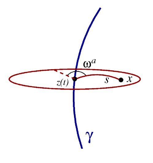
Figure 3: Fermi coordinates.

The Fermi coordinates $(t,x^{a}=s\omega^{a})$ are constructed as follows (LRR Sec. 3.2). We select a point $x$ in a neighbourhood of the world line, and we locate the unique geodesic segment $\beta$ that originates at $x$ and intersects $\gamma$ orthogonally. The intersection point is labeled $\bar{x}$, and $t$ is the value of the proper-time parameter at this point: $\bar{x}=z(\tau=t)$. This defines the time coordinate $t$ of the point $x$. The spatial coordinates $x^{a}$ are defined by

$$x^{a}:=-e^{a}_{\bar{\alpha}}(\bar{x})\sigma^{\bar{\alpha}}(x,\bar{x});$$ (8)

they are the projections in the basis $e^{\bar{\alpha}}_{a}$ of the deviation vector $-\sigma^{\bar{\alpha}}(x,\bar{x})$ between the points $x$ and $\bar{x}$. The Fermi coordinates come with the condition $\sigma_{\bar{\alpha}}(x,\bar{x})u^{\bar{\alpha}}(\bar{x})=0$, which states that the deviation vector is orthogonal to the world line’s tangent vector; it is this condition that identifies the intersection point $\bar{x}=z(t)$.

It is useful to introduce $s$ as the proper distance between $x$ and the world line. This is formally defined by $s^{2}:=2\sigma(x,\bar{x})$, and it is easy to involve the completeness relation and show that $s^{2}=\delta_{ab}x^{a}x^{b}$ (LRR Sec. 3.2.3); the Fermi distance $s$ is therefore the usual Euclidean distance associated with the quasi-Cartesian coordinates $x^{a}$. It is also useful to introduce the direction cosines $\omega^{a}:=x^{a}/s$; these quantities satisfy $\delta_{ab}\omega^{a}\omega^{b}=1$, and they can be thought of as a radial unit vector that points away from the world line.

Each hypersurface $t=\mbox{constant}$ is orthogonal to the world line (in the sense described above), and each spacetime point $x$ within the surface can be said to be simultaneous with $\bar{x}=z(t)$. The Fermi coordinates therefore provide a convenient notion of rest frame for the particle.

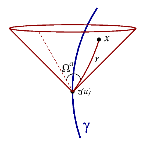
Figure 4: Retarded coordinates.

The retarded coordinates $(u,x^{a}=r\Omega^{a})$ are constructed as follows (LRR Sec. 3.3). Once more we select a point $x$ in a neighbourhood of the world line, but this time we locate the unique null geodesic segment $\beta$ that originates at $x$ and travels backward in time toward $\gamma$. The new intersection point is labeled $x^{\prime}$, and $u$ is the value of the proper-time parameter at this point: $x^{\prime}=z(\tau=u)$. This defines the time coordinate $u$ of the point $x$. The spatial coordinates $x^{a}$ are defined exactly as before, by

$$x^{a}:=-e^{a}_{\alpha^{\prime}}(x^{\prime})\sigma^{\alpha^{\prime}}(x,x^{\prime}).$$ (9)

The retarded coordinates come with the condition $\sigma(x,x^{\prime})=0$, which states that the points $x$ and $x^{\prime}=z(u)$ are linked by a null geodesic (which travels forward in time from $x^{\prime}$ to $x$).

It is useful to introduce $r$ as a measure of light-cone distance between $x$ and the world line. This is formally defined by $r:=\sigma_{\alpha^{\prime}}(x,x^{\prime})u^{\alpha^{\prime}}(x^{\prime})$, and can be shown to be an affine parameter on the null geodesic that links $x$ to $x^{\prime}$ (LRR Sec. 3.3.3). In addition, we have that $r^{2}=\delta_{ab}x^{a}x^{b}$, and $r$ is the usual Euclidean distance associated with the spatial coordinates $x^{a}$. It is also useful to introduce the direction cosines $\Omega^{a}:=x^{a}/r$, which again play the role of a unit radial vector that points away from the world line.

Each hypersurface $u=\mbox{constant}$ is the future light cone of the point $z(u)$ on the world line. Any point $x$ on this light cone is in direct causal contact with $z(u)$. For this reason the retarded coordinates give the simplest description of the scalar field $\Phi$ produced by a point charge $q$ moving on the world line. The field satisfies a wave equation, and the radiation produced by the field essentially realizes the light cones that are so prominently featured in the construction of the coordinates.

4 Field equation and particle motion

Let me recapitulate the problem that we wish to solve. We have a point particle of mass $m$ and scalar charge $q$ moving on a world line $\gamma$ described by the parametric relations $z^{\mu}(\tau)$. The particle creates a scalar field $\Phi(x)$ and this field acts back on the particle and produces a force $F_{\rm self}^{\alpha}$. We wish to determine this self-force.

The scalar field obeys the linear wave equation

$$\Box\Phi=-4\pi\mu,$$ (10)

where $\Box:=g^{\alpha\beta}\nabla_{\alpha}\nabla_{\beta}$ is the wave operator, and

$$\mu(x)=q\int_{\gamma}\delta_{4}\bigl{(}x,z(\tau)\bigr{)}\,d\tau$$ (11)

is the scalar-charge density, expressed as an integral over the world line. The four-dimensional delta function $\delta_{4}(x,z)$ is defined as a scalar quantity; it is normalized by $\int\delta_{4}(x,x^{\prime})\,\sqrt{-g}d^{4}x=1$.

The particle moves according to

$$m(\tau)a^{\mu}=q\bigl{(}g^{\mu\nu}+u^{\mu}u^{\nu}\bigr{)}\Phi_{\nu},$$ (12)

where $a^{\mu}=Du^{\mu}/d\tau$ is the covariant acceleration and $\Phi_{\nu}:=\nabla_{\nu}\Phi$ is the field gradient. The presence of the projector $g^{\mu\nu}+u^{\mu}u^{\nu}$ on the right-hand side ensures that the acceleration is orthogonal to the velocity. The field gradient, however, also has a component in the direction of the world line, and this produces a change in the particle’s rest mass (LRR Sec. 5.1.1): $dm/d\tau=-qu^{\mu}\Phi_{\mu}$. We shall not be concerned with this effect here. Suffice it to say that the mass is not conserved because the scalar field can radiate monopole waves, which is impossible for electromagnetic and gravitational radiation.

The wave equation for $\Phi$ can be integrated, as we shall do in the following section, and the solution can be examined near the world line. Not surprisingly, the field is singular on the world line. This property makes the equation of motion meaningless as it stands, and we shall have to make sense of it in the course of our analysis.

5 Retarded Green’s function

The wave equation for $\Phi$ is solved by means of a Green’s function $G(x,x^{\prime})$ that satisfies

$$\Box G(x,x^{\prime})=-4\pi\delta_{4}(x,x^{\prime}).$$ (13)

The solution is simply

$$\Phi(x)=\int G(x,x^{\prime})\mu(x^{\prime})\,\sqrt{-g^{\prime}}d^{4}x^{\prime}=q\int_{\gamma}G(x,z)\,d\tau,$$ (14)

and the difficulty of solving the wave equation has been transferred to the difficulty of computing the Green’s function. We wish to construct the retarded solution to the wave equation, and this is accomplished by selecting the retarded Green’s function $G_{\rm ret}(x,x^{\prime})$ among all the solutions to Green’s equation. (Other choices will be considered below.) The retarded Green’s function possesses the important property that it vanishes when the source point $x^{\prime}$ is in the future of the field point $x$. This ensures that $\Phi(x)$ depends on the past behaviour of the source $\mu$, but not on its future behaviour.

The retarded Green’s function is known to exist globally as a distribution if the spacetime is globally hyperbolic. But knowledge of the Green’s function is required only in the immediate vicinity of the world line, so as to identify the behaviour of $\Phi$ there; we shall not be concerned with the behaviour of the Green’s function when $x$ and $z(\tau)$ are widely separated.

In this context the Green’s function can be shown (LRR Sec. 4.3) to admit a Hadamard decomposition of the form

$$G_{\rm ret}(x,x^{\prime})=U(x,x^{\prime})\delta_{\rm future}(\sigma)+V(x,x^{\prime})\Theta_{\rm future}(-\sigma),$$ (15)

where $\sigma(x,x^{\prime})$ is the world function introduced previously, and the two-point functions $U(x,x^{\prime})$ and $V(x,x^{\prime})$ are smooth when $x\to x^{\prime}$. The retarded Green’s function is not smooth in this limit, however, as we can see from the presence of the delta and theta functions. The first term involves $\delta_{\rm future}(\sigma)$, the restriction of $\delta(\sigma)$ on the future light cone of the source point $x^{\prime}$. The delta function is active when $\sigma(x,x^{\prime})=0$, and this describes (for fixed $x^{\prime}$) the future and past light cones of $x^{\prime}$. We then eliminate the past branch of the light cone — for example, by multiplying $\delta(\sigma)$ by the step function $\Theta(t-t^{\prime})$ — and this produces $\delta_{\rm future}(\sigma)$. The second term involves $\Theta_{\rm future}(-\sigma)$, a step function that is active when $\sigma<0$, that is, when $x$ and $x^{\prime}$ are timelike related; we also restrict the interior of the light cone to the future branch, so that $x$ is necessarily in the future of $x^{\prime}$.

The delta term in $G_{\rm ret}(x,x^{\prime})$ is sometimes called the direct term, and it corresponds to propagation from $x^{\prime}$ to $x$ that takes place directly on the light cone. If the Green’s function contained a direct term only (as it does in flat spacetime), the field at $x$ would depend only on the conditions of the source $\mu$ at the corresponding retarded events $x^{\prime}$, the intersection between the support of the source and $x$’s past light cone. In the case of a point particle this reduces to a single point $x^{\prime}\equiv z(u)$. The theta term in $G_{\rm ret}(x,x^{\prime})$, which is sometimes called the tail term, corresponds to propagation within the light cone; this extra term (which is generically present in curved spacetime) brings a dependence from events $x^{\prime}$ that lie in the past of the retarded events. In the case of a point particle, the field at $x$ depends on the particle’s entire past history, from $\tau=-\infty$ to $\tau=u$.

There exists an algorithm to calculate $U(x,x^{\prime})$ and $V(x,x^{\prime})$ in the form of Taylor expansions in powers of $-\sigma^{\alpha^{\prime}}$ (LRR Sec. 4.3.2). It returns

$$U(x,x^{\prime})=1+\frac{1}{12}R_{\alpha^{\prime}\beta^{\prime}}\sigma^{\alpha^{\prime}}\sigma^{\beta^{\prime}}+\cdots$$ (16)

and

$$V(x,x^{\prime})=\frac{1}{12}R(x^{\prime})+\cdots,$$ (17)

where $R_{\alpha^{\prime}\beta^{\prime}}$ is the Ricci tensor at $x^{\prime}$, and $R(x^{\prime})$ the Ricci scalar at $x^{\prime}$. In Ricci-flat spacetimes the expansions of $U-1$ and $V$ both begin at the fourth order in $\sigma^{\alpha^{\prime}}$.

6 Alternate Green’s function

The advanced Green’s function is given by (LRR Sec. 4.3)

$$G_{\rm adv}(x,x^{\prime})=U(x,x^{\prime})\delta_{\rm past}(\sigma)+V(x,x^{\prime})\Theta_{\rm past}(-\sigma),$$ (18)

in terms of the same two-point functions $U(x,x^{\prime})$ and $V(x,x^{\prime})$ that appear within the retarded Green’s function. The difference is that the light cones are now restricted to the past branch, so that $G_{\rm adv}(x,x^{\prime})$ vanishes when $x^{\prime}$ is in the past of $x$. A solution to the wave equation constructed with the advanced Green’s function would display anti-causal behaviour: it would depend on the future history of the source.

Another useful choice of Green’s function is the Detweiler-Whiting singular Green’s function defined by (LRR Sec. 4.3.5)

$$G_{\rm S}(x,x^{\prime})=\frac{1}{2}U(x,x^{\prime})\delta(\sigma)-\frac{1}{2}V(x,x^{\prime})\Theta(\sigma).$$ (19)

Here the delta and theta functions are no longer restricted: both future and past branches contribute to the Green’s function. In fact, the argument of the step function is now $+\sigma$, and this indicates that the second term is active when $x$ and $x^{\prime}$ are spacelike related. For fixed $x^{\prime}$, the singular Green’s function is nonzero when $x$ is either on, or outside, the (past and future) light cone of $x^{\prime}$. Unlike the retarded and advanced Green’s functions, $G_{\rm S}(x,x^{\prime})$ is not known to exist globally as a distribution (even for globally hyperbolic spacetimes); its local existence is not in doubt, however, and this suffices for our purposes.

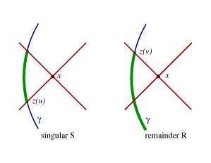
Figure 5: Solutions to the wave equation. The retarded field is sourced by the past history of the point particle, up to the retarded position $z(u)$. The advanced field is sourced by the future history, starting from the advanced position $z(v)$. The singular field is sourced by the world-line segment that lies on and outside the light cone of the field-point $x$, starting from the retarded position $z(u)$ and ending at the advanced position $z(v)$. Finally, the regular field is sourced by the history of the particle up to the advanced position $z(v)$.

All three Green’s functions satisfy the same wave equation, $\Box G=-4\pi\delta_{4}$, and all three give rise to fields $\Phi(x)$ that diverge on the particle’s world line. A useful combination of Green’s functions is the Detweiler-Whiting regular two-point function

$$G_{\rm R}(x,x^{\prime})=G_{\rm ret}(x,x^{\prime})-G_{\rm S}(x,x^{\prime}),$$ (20)

which satisfies the homogeneous wave equation $\Box G_{\rm R}(x,x^{\prime})=0$. This two-point function gives rise to a field

$$\Phi_{\rm R}=\Phi_{\rm ret}-\Phi_{\rm S}$$ (21)

that also satisfies the homogeneous wave equation, $\Box\Phi_{\rm R}=0$. This field is the difference between two singular fields, and since $\Phi_{\rm ret}$ and $\Phi_{\rm S}$ are equally singular near the world line, we find that the regular remainder field $\Phi_{\rm R}$ stays bounded when $x\to z(\tau)$. And what’s more, the regular field is smooth, in the sense that it and any number of its derivatives possess a well-defined limit when $x\to z(\tau)$.

7 Fields near the world line

Using the ingredients presented in the preceding sections it is possible to show (LRR Secs. 5.1.3, 5.1.4, and 5.1.5) that close to the world line, the retarded, singular, and regular fields are given by

$$\Phi_{\rm ret} =\frac{q}{r}+q\int_{-\infty}^{u}V(x,z)\,d\tau+O(r^{2}),$$ (22a)

$$\Phi_{\rm S} =\frac{q}{r}-\frac{1}{3}q\dot{a}_{a}x^{a}+O(r^{2}),$$ (22b)

$$\Phi_{\rm R} =\frac{1}{3}q\dot{a}_{a}x^{a}+q\int_{-\infty}^{u}V(x,z)\,d\tau+O(r^{2}),$$ (22c)

in the retarded coordinates $(u,x^{a}=r\Omega^{a})$. These expressions involve the retarded distance $r$ from $x$ to $z(u)$ and the frame component $\dot{a}_{a}(u):=\dot{a}_{\mu}e^{\mu}_{a}$ of $\dot{a}^{\mu}:=Da^{\mu}/d\tau$, the proper-time derivative of the acceleration vector. They involve also an integration over the past history of the particle. These expressions are valid for Ricci-flat spacetimes. We observe that the retarded and singular fields both diverge as $q/r$ as we approach the world line, but that the regular remainder $\Phi_{\rm R}$ is free of singularities.

In the Fermi coordinates $(t,x^{a}=s\omega^{a})$ we have the more complicated expressions

$$\Phi_{\rm ret} =\frac{q}{s}-\frac{1}{2}qa_{a}\omega^{a}+qs\biggl{(}\frac{1}{8}\dot{a}_{0}+\frac{1}{3}\dot{a}_{a}\omega^{a}-\frac{1}{6}R_{0a0b}\omega^{a}\omega^{b}\biggr{)}$$

$$\qquad\mbox{}+q\int_{-\infty}^{t}V(x,z)\,d\tau+O(s^{2}),$$ (23a)

$$\Phi_{\rm S} =\frac{q}{s}-\frac{1}{2}qa_{a}\omega^{a}+qs\biggl{(}\frac{1}{8}\dot{a}_{0}-\frac{1}{6}R_{0a0b}\omega^{a}\omega^{b}\biggr{)}+O(s^{2}),$$ (23b)

$$\Phi_{\rm R} =\frac{1}{3}q\dot{a}_{a}x^{a}+q\int_{-\infty}^{t}V(x,z)\,d\tau+O(s^{2}).$$ (23c)

They involve the spatial distance $s$ between $x$ and $z(t)$, the frame components of the acceleration vector and its proper-time derivative, the frame components of the Riemann tensor, and the integration over the past history of the particle. Once more we see that the retarded and singular fields diverge in the limit $s\to 0$, but that the regular field is free of singularities. (The singular nature of $\Phi_{\rm S}$ is also observed in a term such as $\frac{1}{2}qa_{a}\omega^{a}$ that stays bounded when $s\to 0$, but is directionally ambiguous on the world line.)

From these equations we may calculate the spatial derivatives of the singular and regular fields. We obtain

$$\nabla_{a}\Phi_{\rm S} =-\frac{q}{s^{2}}\omega_{a}-\frac{q}{2s}\bigl{(}\delta^{b}_{a}-\omega^{b}\omega_{a}\bigr{)}a_{b}+\frac{q}{8}\dot{a}_{0}\,\omega_{a}$$

$$\qquad\mbox{}+\frac{q}{6}R_{0b0c}\,\omega_{a}\omega^{b}\omega^{c}-\frac{q}{3}R_{0a0b}\,\omega^{b}+O(s),$$ (24a)

$$\nabla_{a}\Phi_{\rm R} =\frac{1}{3}q\dot{a}_{a}+q\int_{-\infty}^{t}\nabla_{a}V(x,z)\,d\tau+O(s).$$ (24b)

As expected, the gradient of the singular field diverges as $q/s^{2}$, but the gradient of the regular field is free of singularities. The gradient of the retarded field is $\nabla_{a}\Phi_{\rm ret}=\nabla_{a}\Phi_{\rm S}+\nabla_{a}\Phi_{\rm R}$.

We notice that many terms in $\nabla_{a}\Phi_{\rm S}$ are proportional to an odd number of radial vectors $\omega^{a}$; all such terms vanish when we average the field gradient over a spherical surface of constant $s$. This averaging leaves behind

$$\bigl{\langle}\nabla_{a}\Phi_{\rm S}\bigr{\rangle}=-\biggl{(}\frac{q}{3s}\biggr{)}a_{a}+O(s),$$ (25)

which is still singular. To obtain this result we made use of the identity $\langle\omega^{b}\omega_{a}\rangle=\frac{1}{3}\delta^{b}_{a}$. Notice that because $\nabla_{a}\Phi_{\rm R}$ is smooth at $s=0$, an averaging simply returns the same expression: $\langle\nabla_{a}\Phi_{\rm R}\rangle=\nabla_{a}\Phi_{\rm R}$.

8 Self-force

Let us now reflect on the results of the preceding section and try to make sense of Eq. (12) as an equation of motion for the particle. Our first attempt will be entirely heuristic; we shall add refinement to our treatment in the following section.

Given that Eq. (12) does not make sense as it stands when we insert $\Phi=\Phi_{\rm ret}$ on its right-hand side, let us take the view that the equation is meant to apply to an extended body instead of a point particle, and let us average $\Phi_{\mu}:=\nabla_{\mu}\Phi$ over the body’s volume. This operation should be carried out in the body’s rest frame, and for this purpose it is natural to adopt the Fermi coordinates. We aim, therefore, to average the spatial components $\Phi^{\rm ret}_{a}$ of the field gradient. The simplest form of averaging was carried out already in the preceding section, and we obtained

$$\langle\Phi^{\rm ret}_{a}\rangle=\langle\Phi^{\rm S}_{a}\rangle+\langle\Phi^{\rm R}_{a}\rangle=-\biggl{(}\frac{q}{3s}\biggr{)}a_{a}+\Phi^{\rm R}_{a}+O(s),$$ (26)

in which $\Phi^{\rm R}_{a}$ is evaluated (without obstacle) at $s=0$. This expression corresponds to pretending that the body is a thin spherical shell of radius $s$.

Substitution into Eq. (12) and evaluation in the Fermi coordinates produces

$$(m+\delta m)a^{a}=q\Phi_{\rm R}^{a},$$ (27)

with $\delta m:=q^{2}/(3s)$ denoting the contribution to the total body mass that comes from the field’s energy. Absorbing this into a redefinition of the inertial mass $m$, the final tensorial expression for the equation of motion is

$$ma^{\alpha}=q\bigl{(}g^{\alpha\beta}+u^{\alpha}u^{\beta}\bigr{)}\nabla_{\beta}\Phi_{\rm R},$$ (28)

with

$$\nabla_{\beta}\Phi_{\rm R}=\frac{1}{3}q\dot{a}_{\beta}+q\int_{-\infty}^{\tau}\nabla_{\beta}V(x,z)\,d\tau^{\prime}.$$ (29)

This is Quinn’s equation of motion quinn:00 for a scalar charge $q$ moving in a curved spacetime with metric $g_{\alpha\beta}$. The self-force involves an instantaneous term proportional to $\dot{a}^{\alpha}=Da^{\alpha}/d\tau$, as well as an integral over the particle’s past history.

Equation (28) informs us that of the complete retarded field $\Phi_{\rm ret}=\Phi_{\rm S}+\Phi_{\rm R}$, only the Detweiler-Whiting regular field $\Phi_{\rm R}$ contributes to the self-force. The role of the singular field is merely to contribute to the particle’s inertia, through a shift $\delta m$ in its inertial mass. This contribution diverges in the limit $s\to 0$, but it would be finite for any extended body.

I must confess that this computation returns the wrong expression for the particle’s self-energy. We obtained $\delta m=q^{2}/(3s)$, while the correct expression is $\delta m=q^{2}/(2s)$; we are wrong by a factor of $2/3$. I believe that this discrepancy originates in an inconsistency between our assumed shape for the extended body — a spherical shell of radius $s$ — and the field it produces, which we took to be equal to the field produced by a point particle. I would conjecture that calculating the field actually produced by a spherical shell would give rise to the correct expression for $\delta m$, but leave unchanged the final result of Eq. (28) for the equation of motion.

9 Axiomatic approach

The procedure outlined above is admittedly heuristic. It can, however, be formalized and put on an axiomatic basis that supplies Eq. (28) with a much improved pedigree. This is the approach that was first pursued by Ted Quinn and Bob Wald quinn-wald:97 ; quinn:00 . They formulate two axioms that the scalar self-force $F^{\alpha}$ should satisfy:

Quinn-Wald Axiom 1.

Two scalar particles move on world lines $\gamma$ and $\tilde{\gamma}$ in two different spacetimes. At points $z$ and $\tilde{z}$ their acceleration vectors have equal lengths. The neighbourhoods of $z$ and $\tilde{z}$, as well as the acceleration vectors, are identified in Fermi coordinates. Then the difference in the self-forces is given by

$$F^{\alpha}-\tilde{F}^{\alpha}=q\bigl{(}g^{\alpha\beta}+u^{\alpha}u^{\beta}\bigr{)}\lim_{s\to 0}\Bigl{\langle}\Phi_{\beta}-\tilde{\Phi}_{\beta}\Bigr{\rangle}.$$ (30)

Here $\Phi$ and $\tilde{\Phi}$ are the retarded fields in each spacetime, and $\Phi_{\beta}:=\nabla_{\beta}\Phi$ while $\tilde{\Phi}_{\beta}:=\tilde{\nabla}_{\beta}\tilde{\Phi}$. The limit is well defined after the difference of field gradients is averaged over a sphere of radius $s$.

Quinn-Wald Axiom 2.

$\tilde{F}^{\alpha}=0$ in flat spacetime, for a particle with uniform acceleration.

The first axiom is essentially a statement that when two particles momentarily share the same acceleration, their fields are equally singular, and the difference (after averaging) possesses a well-defined limit when $s\to 0$. The second axion is a scalar-charge analogue to a well-known result from flat-spacetime electrodynamics: a charged particle moving with a uniform acceleration does not undergo radiation reaction.

According to Eqs. (24), the curved-spacetime expression for the gradient of the retarded field is

$$\Phi_{a} = -\frac{q}{s^{2}}\omega_{a}-\frac{q}{2s}\bigl{(}\delta^{b}_{a}-\omega^{b}\omega_{a}\bigr{)}a_{b}+\frac{q}{8}\dot{a}_{0}\,\omega_{a}$$ (31)

$$\mbox{}+\frac{q}{6}R_{0b0c}\,\omega_{a}\omega^{b}\omega^{c}-\frac{q}{3}R_{0a0b}\,\omega^{b}+\nabla_{a}\Phi_{\rm R}+O(s);$$

this holds at time $t$ in Fermi coordinates. The flat-spacetime expression is

$$\tilde{\Phi}_{a}=-\frac{q}{s^{2}}\omega_{a}-\frac{q}{2s}\bigl{(}\delta^{b}_{a}-\omega^{b}\omega_{a}\bigr{)}a_{b}+O(s),$$ (32)

and this also holds at time $t$ in the same system of Fermi coordinates. Under the conditions of the Quinn-Wald axioms, the acceleration $a_{a}$ that appears in $\Phi_{a}$ and $\tilde{\Phi}_{a}$ is one and the same. In the flat-spacetime expression we set $\dot{a}_{0}$ and $\dot{a}_{a}$ to zero because the acceleration is chosen to be uniform. In addition we eliminate the Riemann-tensor terms, as well as the integral over the particle’s past history — $V$ necessarily vanishes in flat spacetime.

Subtraction yields

$$\Phi_{a}-\tilde{\Phi}_{a}=\frac{q}{8}\dot{a}_{0}\,\omega_{a}+\frac{q}{6}R_{0b0c}\,\omega_{a}\omega^{b}\omega^{c}-\frac{q}{3}R_{0a0b}\,\omega^{b}+\nabla_{a}\Phi_{\rm R}+O(s),$$ (33)

and we get

$$\bigl{\langle}\Phi_{a}-\tilde{\Phi}_{a}\bigr{\rangle}=\nabla_{a}\Phi_{\rm R}+O(s)$$ (34)

after averaging over a sphere of constant $s$. The difference in the self-forces is therefore $F_{a}-\tilde{F}_{a}=q\nabla_{a}\Phi_{\rm R}$. The second axiom finally returns $F_{a}=q\nabla_{a}\Phi_{\rm R}$, which is equivalent to Eq. (28); we have reproduced Quinn’s expression for the scalar self-force. Notice that the second axiom eliminates the need to carry out an explicit renormalization of the mass.

Another axiomatic approach provides an even more immediate derivation of Quinn’s equation. This is the approach suggested by Steve Detweiler and Bernard Whiting detweiler-whiting:03 , which is based on an observation and an alternate axiom:

Detweiler-Whiting Observation.

The retarded field $\Phi_{\rm ret}$ can be decomposed uniquely into a singular piece $\Phi_{\rm S}$ and a regular remainder $\Phi_{\rm R}$.

Detweiler-Whiting Axiom.

The singular field produces no force on the particle.

The immediate consequence of the axiom is that only the regular field participates in the self-force, and we once more arrive at Quinn’s equation.

The Detweiler-Whiting approach is very clean and provides a quick route to the final answer. The observation is not at all controversial, because the singular field is indeed uniquely defined by the prescription outlined in Sec. 6. The axiom, on the other hand, seems too good to be true. How can it just be asserted that the singular field produces no force?

A fairly compelling line of argument rests on the fact that according to its definition, the singular field is strongly time-symmetric, in the sense that the field at $x$ does not depend on the future nor the past of the spacetime point; it instead depends on source points $x^{\prime}$ that are in a spacelike or lightlike relation with $x$. Since we would expect the self-force to be sensitive to the direction of time — an advanced field should produce a different force from a retarded field — it seems plausible that the singular field would not know whether to push or pull, and would therefore choose to do neither.

The argument is not water-tight. For example, an alternate singular field, defined by Dirac’s prescription $\frac{1}{2}\Phi_{\rm ret}+\frac{1}{2}\Phi_{\rm adv}$, would also be time-symmetric (though not strongly time-symmetric), and could also be asserted to produce no force. The resulting self-force, however, would be produced by $\frac{1}{2}\Phi_{\rm ret}-\frac{1}{2}\Phi_{\rm adv}$, and would depend on the entire history of the particle, both past and future. We would of course reject this candidate self-force on grounds of causality violation, but the argument nevertheless shows that there is more to the Detweiler-Whiting singular field than a time-symmetry property. Another hole in the argument lies in the link between the time-symmetry of the singular field and the statement that it must exert no force: While the time-symmetry property clearly implies that the singular field cannot produce dissipative effects on the particle, there is no reason to rule out an eventual conservative contribution to the self-force.

The conclusion is that additional axioms are necessarily required to make sense of the equations of motion formulated for a point particle. The axioms may seem plausible and perhaps even self-evident, but they cannot be derived from first principles in the context of a classical field theory coupled to a point particle. Such a theory is inherently singular and ambiguous, and it necessarily requires external input in the form of additional axioms.

10 Conclusion

Can one do better than this? The answer is ‘no’ if we insist in treating the point particle as a fundamental classical object. The answer, however, is ‘yes’ if we properly understand that a point particle is merely a convenient substitute for what is fundamentally an extended body. In this view, the length scale of the moving body is $\ell$, not zero. The body possesses a finite density of scalar charge, the scalar field is finite everywhere, and its motion traces a world tube in spacetime instead of a single world line. To determine this motion is a well-posed problem, but the description now involves a lot of additional details. Under usual circumstances, however, $\ell$ is much smaller than all other length scales present in the problem, such as the radius of curvature ${\cal R}$ of the body’s trajectory. Under these circumstances the description of the motion can be simplified so as to involve a much smaller number of variables; in the limit $\ell/{\cal R}\to 0$ only the position of the center-of-mass matters, and all couplings between the body’s multipole moments and the external field become irrelevant. In this limit we recover a point-particle description, with the essential understanding that it is merely an approximate description that should not be considered to be fundamental.

To go through the details of this program is difficult, and it appears that very few authors have attempted it since the old days of Lorentz and Abraham. For a recent discussion, and a review of this literature, see the work by Harte harte:06 . Another important exception concerns the gravitational self-force acting on a small black hole (LRR Sec. 5.4), which is decidedly not treated as a point mass.

It is well known that in general relativity, the motion of gravitating bodies is determined, along with the spacetime metric, by the Einstein field equations; the equations of motion are not separately imposed. This observation provides a means of deriving the gravitational self-force without having to rely on the fiction of a point mass. In the powerful method of matched asymptotic expansions, the metric of the small black hole, perturbed by the tidal gravitational field of the external spacetime, is matched to the metric of the external spacetime, perturbed by the black hole. The equations of motion are then recovered by demanding that the metric be a valid solution to the vacuum field equations. In my opinion, this method (which was first applied to the gravitational self-force problem by Mino, Sasaki, and Tanaka mino-etal:97 ) gives what is by far the most compelling derivation of the gravitational self-force. Indeed, the method is entirely free of conceptual and technical pitfalls — there are no singularities (except deep inside the black hole) and only retarded fields are employed.

In this assessment I respectfully disagree with my colleague Bob Wald, who finds that the method incorporates a number of unjustified assumptions. I would concede that expositions of the method — including my own in LRR — might not have sufficiently clarified some of its subtle aspects. But I see this as faulty exposition, not as an intrinsic difficulty with the method of matched asymptotic expansions. I refer the reader to the recent work by Sam Gralla and Bob Wald gralla-wald:08 for their views on this issue, and their own approach to the motion of an extended body in general relativity.

The introduction of a point particle in a classical field theory appears at first sight to be severely misguided. This is all the more true in a nonlinear theory such as general relativity. The lesson learned here is that surprisingly often, one can get away with it. The derivation of the gravitational self-force based on the method of matched asymptotic expansions does indeed show that the result obtained on the basis of a point-particle description can be reliable, in spite of all its questionable aspects. This is a remarkable observation, and one that carries a lot of convenience: It is indeed much easier to implement the point-mass description than to perform the matching of two metrics in two coordinate systems. The lesson, of course, carries over to the scalar and electromagnetic cases.

- (1) E. Poisson, Living Rev. Relativity 7 (2004). 6. [Online article]: cited on , http://www.livingreviews.org/lrr-2004-6
- (2) H. Spohn, Dynamics of charged particles and their radiation field (Cambridge University Press, Cambridge, 2008)
- (3) P.A.M. Dirac, Proc. Roy. Soc. London A167, 148 (1938)
- (4) B.S. DeWitt, R.W. Brehme, Ann. Phys. (N.Y.) 9, 220 (1960)
- (5) J.M. Hobbs, Ann. Phys. (N.Y.) 47, 141 (1968)
- (6) Y. Mino, M. Sasaki, T. Tanaka, Phys. Rev. D 55, 3457 (1997). ArXiv:gr-qc/9606018
- (7) T.C. Quinn, R.M. Wald, Phys. Rev. D 56, 3381 (1997). ArXiv:gr-qc/9610053
- (8) T.C. Quinn, Phys. Rev. D 62, 064029 (2000). ArXiv:gr-qc/0005030
- (9) J.L. Synge, Relativity: The General Theory (North-Holland, Amsterdam, 1960)
- (10) K.S. Thorne, J.B. Hartle, Phys. Rev. D 31, 1815 (1985)
- (11) X.H. Zhang, Phys. Rev. D 34, 991 (1986)
- (12) S. Detweiler, Class. Quantum Grav. 22, S681 (2005). ArXiv:gr-qc/0501004
- (13) S. Detweiler, B.F. Whiting, Phys. Rev. D 67, 024025 (2003). ArXiv:gr-qc/0202086
- (14) A.I. Harte, Phys. Rev. D 73, 065006 (2006). ArXiv:gr-qc/0508123
- (15) S.E. Gralla, R.M. Wald, Class. Quantum Grav. 25, 205009 (2008). ArXiv:0806.3293