Transient Dynamics of Confined Charges in Quantum Dots in the Sequential Tunnelling Regime

Abstract

We investigate the time-dependent, coherent, and dissipative dynamics of bound particles in single multilevel quantum dots in the presence of sequential tunnelling transport. We focus on the nonequilibrium regime where several channels are available for transport. Through a fully microscopic and non-Markovian density matrix formalism we investigate transport-induced decoherence and relaxation of the system. We validate our methodology by also investigating the Markov limit on our model. We confirm that not only does this limit neglect the coherent oscillations between system states as expected, but also the rate at which the steady state is reached under this limit significantly differs from the non-Markovian results. By a systematic analysis of the decay constants and frequencies of coherent oscillations for the off-diagonal elements of the reduced density matrix under various realistic tunneling rate anisotropies and energy configurations, we outline a criteria for extended decoherence times.

I Introduction

It is a fundamental feature of quantum theory that the dynamics of an isolated system will follow a unitary evolution, and thus be fully reversible. In practice, most quantum systems are influenced by uncontrolled and inevitable interactions with an often incoherent environment, and this influence will typically destroy this deterministic evolution and result in the rapid vanishing of any quantum coherence within the open system. Breuer and Petruccione (2002)

A large body of theoretical work has been carried out throughout the last half century which has pushed forward the investigation of the dynamics of open quantum systems (OQS). The seminal work by Nakajima Nakajima (1958) and Zwanzig Zwanzig (1960) on projection operator methods, as well as the works by Kraus, Kraus (1971) Lindblad, Lindblad (1976) and Gorini, Kossakowki, and Sudarshan Gorini et al. (1976) on quantum dynamical semigroups, and by Davies Davies (1974) on Markovian master equations, have rigorously established the conditions for positivity of physical probabilities in open quantum systems. Since then, Markovian approaches have been successfully used Suárez et al. (1992) to study steady state phenomena on open systems where the past memory of the system is neglected, or on closed unitary systems, where the dynamics are deterministic and thus reversible.

The advent of technological applications for quantum coherence, such as in quantum information processing and cryptography, as well as the use of ultrafast laser pulse excitations, are requiring resolutions of the quantum dynamics of a system down to a femtosecond timescale. Shah (1999) This transient regime, which carries the coherence and relaxation dynamics, cannot in general be described by a coarse-grained Markovian limit, mar and a non-Markovian approach is usually necessary. On this point there has been significant progress in recent years; the application of non-Markovian theories to formal physical models in the area of low-dimensional dynamical quantum systems has been extraordinarily fruitful. For example, electron transport by means of full counting statistics, Braggio et al. (2006); Bagrets et al. (2006) current and shot noise analysis by diagrammatic techniques, Thielmann et al. (2005) qubit dynamics in the presence of 1/f noise, Burkard (2009) decoherence of qubit systems by means of effective Hamiltonians for the reservoir, Lee et al. (2004) electron spin dynamics in quantum dots, Coish and Loss (2004) and decoherence in ballistic nanostructures by projector operator techniques, Knezevic (2008) and transient currents through quantum dots by means of the reduced density operator formalism. Moldoveanu et al. (2009)

Formalisms based on non-equilibrium Green’s functions (NEGF) have also been successful in the analysis of much phenomena in mesoscopic systems. Kadanoff and Baym (1962); Haug and Koch (1990); Haug and Jauho (1996) Notably, work in both elastic and inelastic transport in quantum dots has been carried out by means of NEGF or derivatives of this formalism. Wacker and Jauho (1998); Wacker et al. (1999) However, NEGF is inherently a closed-system formalism where the system has Hamiltonian dynamics, Datta (1995) and thus does not account for irreversibility arising from interactions with an unseen, unknown, or otherwise intractable environment. Promising advances have been made to extend NEGF to OQS, for example, by treating the environment as a correction to the system’s self-energy, Datta (2000) or by calculating two-time correlation functions, Knezevic and Ferry (2003) effectively separating the time scales into transient and steady-state regimes. These and other approaches constitute significant progress toward a full non-Markovian open system analysis within the NEGF formalism. 

Even so, when the evolution of the many-body system states themselves are sought, one must calculate the Green’s functions and then extract the density matrix, which in the non-equilibrium case may not be unique. Knezevic and Ferry (2003) An alternative formulation, one we adopt in the present paper, is to work with the reduced density matrix (RDM) directly. This arguably provides a more intuitive description of the dynamics of non-Markovian OQS, and it readily yields the actual states of the system and quantum coherence between them.

Although the works cited above have covered a tremendous amount of ground, to our knowledge there has not been a systematic analysis of the effects of diverse energy and coupling regimes on the quantum coherence in an OQS under the presence of transport-induced relaxation. Thus, the aim of this paper is to investigate the effects of varying energy and coupling parameters on the non-Markovian dynamics of a single few-electron open quantum dot under the RDM formalism. We focus on the sequential transport regime where two or more channels are available for transport, and solve the RDM for the system for the occupation probabilities and quantum coherence to determine energy and coupling regimes leading to larger decoherence times.

This paper is outlined as follows: In section II we derive the evolution equations for the density matrix of the OQS in the Born approximation, and a brief description of the Markov limit is given for completeness. Section III develops the non-Markovian transport theory for a single quantum dot nanostructure coupled to semiinfinite leads. The tunnelling Hamiltonian for the transport model and the assumptions made for the system and reservoirs are described in Sec. III.1. Section III.2 presents in detail the derivation of the analytical expressions for the transition matrix (the memory kernel) containing the dynamics for this model. In Sec. IV we illustrate the non-Markovian approach by considering the case of a multilevel dot in a regime where two channels are available for transport. The analytical expressions for the elements of the RDM are shown in Sec. IV.1, and results are compared with the Markov limit under a variation coupling anisotropy to different orbitals in the quantum dot. The off-diagonal elements representing the coherence in the system are presented in Sec. IV.2, as well as a thorough analysis of the effects of varying the dominant energy and coupling parameters for this model. A summary of the results of the variations of the energy and coupling parameters is given in Sec. IV.3. Finally, conclusions are presented in Sec. V.

II Dynamics of the Open Quantum System

We concentrate on the dynamics of an OQS which does not in general follow a unitary evolution, and where an inherent irreversibility may arise due to coupling with an essentially Markovian (memoryless) environment. When information is continually exchanged between an OQS and an environment whose degrees of freedom are either unknown, intractable, or uninteresting, the (possibly mixed) states of the system alone are described not by state vectors, but rather by the RDM of the system Blum (1996). The RDM can be obtained by taking a partial trace over the degrees of freedom of the environment on the total density matrix for the OQS plus environment, such that

$$\rho(t)=Tr_{\text{env}}[\sigma(t)]=\sum_{n}W_{n}(t)|\psi_{n}(t)\rangle\langle\psi_{n}(t)|$$ (1)

is the RDM of the system, $\sigma(t)$ is the total density matrix, and $W_{n}(t)$ is the probability that the system state $|\psi_{n}(t)\rangle$ is occupied at time $t$.

For Eq. (1) to represent a physical system, where the diagonal elements describe the occupation probabilities and the off-diagonal elements describe the coherence between the OQS states, we require $\rho_{ii}(t)>0$, as well as $|\rho_{i,j}(t)|\leq 1$ for all $i$ and $j$.rho

The partial trace over the degrees of freedom of the environment has the benefit of accounting for the influence of the environment on the OQS, but it also has the drawback of only allowing for limited or average environment descriptions. Although partial-trace-free approaches have been developed Knezevic and Ferry (2002), to our knowledge they have only addressed the steady state regime where memory effects have been neglected.

Considering an environment with a much greater number of degrees of freedom relative to those of the system, and for weak OQS-environment coupling in a sequential tunneling regime (Born approximation), we can assume that the system has negligible effect (no back-action) on the environment, that the system is not correlated with the environment, and that the environment is essentially in equilibrium at all times. Blum (1996) In this case, the total density matrix for the OQS plus environment can be written as

$$\sigma(t)\approx\rho(t)\otimes\varrho(0).$$ (2)

where $\varrho(0)$ is the environment’s equilibrium density matrix.

The dynamics of the RDM in the Born approximation can be obtained by an iterative integration of the Liouville-von Neumann equation to obtain the time dependence for higher order processes, Breuer and Petruccione (2002)

$$\dot{\rho}(t)= -\mathcal{L}(t)\rho(0)+\int_{0}^{t}\!dt^{\prime}\mathcal{L}(t)\mathcal{L}(t^{\prime})\rho(t^{\prime}),$$

where $\mathcal{L}(t)\mathcal{O}=i\hbar^{-1}[H(t),\mathcal{O}]$ is a Liouville superoperator for any operator $\mathcal{O}$ and Hamiltonian $H(t)$.

The matrix elements of the above generalized master equation for the RDM in the interaction picture can be written in the form Blum (1996)

$$\dot{\rho}_{ab}(t)=\sum_{c,d}\int_{0}^{t}\!dt^{\prime}\rho_{cd}(t^{\prime})R_{abcd}(t-t^{\prime})e^{i\gamma_{abcd}t^{\prime}},$$ (4)

where, $R_{abcd}(t-t^{\prime})$ is the memory kernel characterizing the system, the environment, and their coupling, and where $\gamma_{abcd}=\omega_{ab}-\omega_{cd}$, with $\omega_{ab}=(E_{a}-E_{b})/\hbar$ denoting energy differences between OQS states.

The system of coupled integrodifferential convolution equations, Eq. (4), is solved by transforming it into an algebraic system of equations in Laplace space,

$$\sum_{cd}\mathcal{W}_{abcd}(s)~{}\tilde{\rho}_{ab}(s)=\tilde{\rho}_{cd}(0).$$ (5)

where,

$$\mathcal{W}_{abcd}(s)=\left[\delta_{ca}\delta_{bd}\left(s+i\omega_{ab}\right)-\tilde{R}_{abcd}(s)\right]$$

$$\tilde{\rho}_{ab} (t)\equiv\rho_{ab}(t)e^{-i\omega_{ab}t},\ \ \tilde{R}_{abcd}(t)\equiv R_{abcd}(t)e^{-i\omega_{ba}t}.$$

For a given set of basis states, an inverse Laplace transform of Eqn. (5) yields the time dependent solutions in the Heisenberg picture.

Analytic solutions in Laplace-space can be obtained for only a few OQS states ($\sim 2-4$), since the computational effort rapidly increases with the number of available transport channels. For larger numbers of channels, we adopt a numerical approach to solve the linear system in Eq. (5).

In the regime of sequential tunnelling transport through a quantum dot containing uncorrelated electrons, the important transport channels are those single-particle system states $|\alpha\rangle$, whose energy lies within the bias window. These single-particle states define the possible dynamical many-body states of the system as those involved when the single particle states are empty or occupied. Thus, for $k$ channels, a minimum of $2^{k}$ many-body system states are required (for empty or occupied). Furthermore, $(2^{k})^{2}$ density-matrix elements are required to describe the population probabilities as well as the coherence between the states. The temporal evolution of the density-matrix elements themselves are governed by $(2^{k})^{4}$ transition tensor elements. In practice, symmetry considerations can reduce this number only by a constant amount (for details see Ref. [Blum, 1996] pg. 292).

For the results in the following sections we perform the inverse Laplace transform in the form of a Bromwich integral Abramowitz and Stegun (1964) over a contour chosen such that all singularities are to the left of the contour line. The integration is numerically performed int at each time step using a combination of a 25-point Clenshaw-Curtis and a 15-point Gauss-Kronrod integration method.

Markov Limit

We validate the use of a non-Markovian approach by a brief comparison with the long-time Markov limit. Blum (1996) This approximation assumes that the environment correlation functions vanish at such a fast rate that the reversibility, and thus memory of the OQS is essentially destroyed. Breuer and Petruccione (2002) In such a case, $\dot{\rho}(t)$ becomes local in time.

$$\dot{\rho}_{ab}(t)\longrightarrow\sum_{c,d}\rho_{cd}(t)\int_{0}^{t}\!dt^{\prime}R_{abcd}(t-t^{\prime})e^{i\gamma_{abcd}t^{\prime}}.$$ (6)

For time intervals $t-t^{\prime}$ much greater than the environment’s correlation time $\tau$, the correlation functions for environment operators rapidly become uncorrelated and decay to zero, $\langle F_{k}^{\dagger}(t-t^{\prime})F_{k^{\prime}}\rangle\approx\langle F_{k}^{\dagger}(t-t^{\prime})\rangle\langle F_{k^{\prime}}\rangle\approx 0$. Since the environment is uncorrelated beyond this $t-t^{\prime}\gg\tau$ time, there are no contributions to the dynamics, and the upper integration limit in (6) may be extended to infinity with negligible error in the calculations. The lower integration limit of Eq. (6) can be taken to negative infinity, and the memory kernel becomes a delta function of the channel energies. This leads to a Fermi’s Golden rule for transitions with strict energy conservation. Thus, the coupled set of integro-differential evolution equations become a coupled set of first order ordinary differential equations,

$$\dot{\rho}_{ab}(t)=\sum_{c,d}W_{abcd}~{}\rho_{cd}(t),$$ (7)

where $W_{abcd}$ is a time-local transition rate.

The Markov approximation is typically valid only in the long-time limit and leads to a zero-average of the off-diagonal elements of the OQS, thus the transition rates $W_{abcd}$ can be written as $W_{aabb}\equiv W_{ab}$, since only transitions between diagonal elements become relevant.

In the following sections we verify the validity of the Markov limit only once the system has established a steady state Suárez et al. (1992), and that both the approach and relaxation times to the steady state in this limit are unreliable.

III Dynamics in a Single Quantum Dot

III.1 Transport Model

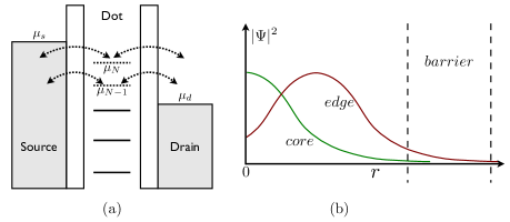
Figure 1: (color online) (a) Schematic representation of the single QD model coupled to source and drain reservoirs. Two transport channels are present within the bias window. (b) Representation of a orbital asymmetry where edge ($p$-type) orbitals are more strongly coupled to the reservoir compared to core ($s$-type) orbitals.

We consider a sequential transport model for a single quantum dot coupled to semiinfinite leads as depicted in Fig. 1a. The total Hamiltonian describing this coupled system plus environment is given by,

$$H=H_{S}+H_{QD}+H_{D}+\mathcal{H}_{T},$$ (8a)

where $$H_{S} H_{D} V_{B}$$ and are the Hamiltonians describing the source and drain leads, respectively. These are taken to be non-interacting Fermion systems shifted by the bias voltage :

$$H_{S(D)}=\sum_{s(d)}(\epsilon_{s(d)}\pm\frac{1}{2}eV_{B})d^{\dagger}_{s(d)}d_{s(d)},$$ (8b)

with $$d^{\dagger}_{s(d)} d_{s(d)}$$ a creation operator for the source (drain), and an annihilation operator.

The Hamiltonian for the quantum dot in Eq.(8a) is given by,

$$H_{QD}=\sum_{i}(\hbar\omega_{i}+eV_{g})c^{\dagger}_{i}c_{i}+V_{\mathrm{int}},$$ (8c)

where $c^{\dagger}_{i}$ and $c_{i}$ are system creation and annihilation operators, the single-particle energies $\hbar\omega_{i}$ are all shifted by the applied gate voltage, $V_{g}$, and $V_{\mathrm{int}}$ is the interaction among the confined particles. In the present work we set $V_{\mathrm{int}}=0$. Although we expect our qualitative results to remain unchanged, the implications of a full coulomb interaction in this transport theory may have significant consequences and will be the subject of future work.

The tunneling Hamiltonian describing the coupling between the reservoirs and the dot is given by, Mahan (1981)

$$\mathcal{H}_{T}=\sum_{k,r=(s,d)}\left(T^{r}_{k}d^{\dagger}_{r}c_{k}+h.c\right),$$ (8d)

where $T^{s(d)}_{k}$ is a tunneling coefficient for a particle tunneling from the single-particle state $|k\rangle$ in the dot to the source (drain) reservoir. For the present model, we assume a small level broadening $\Gamma$, and low temperature such that $\Gamma\ll k_{B}T\ll\Delta E$. In this case the reservoirs are in their respective non-degenerate ground states.

III.2 Memory Kernel

In order to obtain the system dynamics for this transport model, we derive the memory kernel $R_{abcd}(t)$ appearing in Eq. (4). By evaluating the Liouville superoperator appearing in Eq. (II) in the interaction picture, and within the weak interaction limit to second order in Eq. (8d), the time evolution of the RDM becomes,

$$\dot{\rho}(t)=- \frac{i}{\hbar}Tr_{\mathcal{B}}[\mathcal{H}_{T}(t),\rho(0)\varrho(0)]$$

$$- \frac{1}{\hbar^{2}}\int_{0}^{t}dt^{\prime}Tr_{\mathcal{B}}[\mathcal{H}_{T}(t),[\mathcal{H}_{T}(t^{\prime}),\rho(t^{\prime})\varrho(0)]].$$ (9)

The tunneling Hamiltonian (8d) can be rewritten in the form,

$$\mathcal{H}_{T}(t)=\sum_{k}\left(F_{k}(t)Q^{\dagger}_{k}(t)+F^{\dagger}_{k}(t)Q_{k}(t)\right),$$ (10)

where $Q_{i}(t)=e^{iH_{QD}t}c_{i}e^{-iH_{QD}t}$, and where

$$F_{k}(t)=\sum_{s}T^{S}_{k,s}L_{s}(t)+\sum_{d}T^{D}_{k,d}L_{d}(t)$$ (11)

is a generalized reservoir operator that takes into account both source and drain reservoir states, where $L_{s(d)}(t)=e^{iH_{S(D)}t}d_{s(d)}e^{-iH_{S(D)}t}$.

Noting that the interaction Hamiltonian has zero expectation with respect to the equilibrium ensemble of the environment, we have that

$$Tr_{R}[F_{k}(t)\varrho(0)]=\langle F_{k}(t)\rangle=0,$$ (12)

$$\langle F_{k}(t)F_{k^{\prime}}(t^{\prime})\rangle=\langle F^{\dagger}_{k}(t)F^{\dagger}_{k^{\prime}}(t^{\prime})\rangle=0.$$

Thus, the odd moments of $\mathcal{H}_{T}$ as defined in Eq. (11) with respect to the density matrix for the equilibrium reservoir will all vanish.

With Eq. (12), the evolution equation (Eq. (III.2)) becomes

$$\dot{\rho}( t)=-\frac{1}{\hbar^{2}}\sum_{i,j}\int_{0}^{t}dt^{\prime}$$

$$\left\{\left(Q_{i}(t)Q^{{\dagger}}_{j}(t^{\prime})\rho(t^{\prime})-Q^{{\dagger}}_{j}(t^{\prime})\rho(t^{\prime})Q_{i}(t)\right)\langle F^{{\dagger}}_{i}(t)F_{j}(t^{\prime})\rangle\right.$$

$$+ \left(\rho(t^{\prime})Q_{i}(t)Q^{{\dagger}}_{j}(t^{\prime})-Q_{i}(t)\rho(t^{\prime})Q^{{\dagger}}_{j}(t^{\prime})\right)\langle F_{i}(t)F^{{\dagger}}_{j}(t^{\prime})\rangle$$

$$+ \left(\rho(t^{\prime})Q_{j}(t^{\prime})Q^{{\dagger}}_{i}(t)-Q^{{\dagger}}_{i}(t)\rho(t^{\prime})Q_{j}(t^{\prime})\right)\langle F^{{\dagger}}_{j}(t^{\prime})F_{i}(t)\rangle$$

$$+ \left.\left(Q^{{\dagger}}_{i}(t)Q_{j}(t^{\prime})\rho(t^{\prime})-Q_{j}(t^{\prime})\rho(t^{\prime})Q^{{\dagger}}_{i}(t)\right)\langle F_{i}(t)F^{{\dagger}}_{j}(t^{\prime})\rangle\right\},$$ (13)

A matrix element of the first term on the right of (III.2) (where there are 8 terms in total) can be rewritten in the following way,

$$\langle m^{\prime} |Q_{i}(t)Q^{{\dagger}}_{j}(t^{\prime})\rho(t^{\prime})|m\rangle=$$

$$=\sum_{n,n^{\prime},k}\delta_{mn^{\prime}}\langle m^{\prime}|Q_{j}|k\rangle\langle k|Q^{{\dagger}}_{i}(\tau)|n\rangle\langle n|\rho(t^{\prime})|n^{\prime}\rangle e^{i\Omega^{m^{\prime}n}_{mn^{\prime}}t},$$ (14)

where $\Omega^{m^{\prime}n}_{mn^{\prime}}=(E_{m^{\prime}}-E_{n}+E_{n^{\prime}}-E_{m})$, $\tau=t-t^{\prime}$, and where the RDM elements have been rewritten as,

$$\rho_{n^{\prime},m}(t)=\sum_{n}\delta_{n,m}\rho_{n^{\prime},n}(t)e^{i\omega_{n,m}t}.$$ (15)

Terms 3,5,7 in the right side of (III.2) can be written in a similar way.

The elements of the second term in (III.2) can be rewritten as,

$$\langle m^{\prime}|Q_{i}(t)\rho(t^{\prime})Q^{{\dagger}}_{j}(t^{\prime})|m\rangle=$$

$$\sum_{n,n^{\prime},k}\delta_{m,n^{\prime}}\langle m^{\prime}|Q_{j}|k\rangle\langle k|Q^{{\dagger}}_{i}(\tau)|n\rangle\langle n|\rho(t^{\prime})|n^{\prime}\rangle e^{i\Omega^{m^{\prime},n}_{m,n^{\prime}}t},$$ (16)

and similarly for terms 2,6,8 in (III.2).

The reservoir operator $F_{i}$ has no explicit time dependence; we can therefore write, $\langle F^{\dagger}_{\alpha}(t)F_{\beta}(t^{\prime})\rangle=\langle F^{\dagger}_{\alpha}F_{\beta}(\tau)\rangle$, and $\langle F^{\dagger}_{\beta}(t^{\prime})F_{\alpha}(t)\rangle=\langle F^{\dagger}_{\beta}(\tau)F_{\alpha}\rangle$.

Finally, for a given quantum dot state, we allow coupling with all available reservoir states, while treating the reservoir energy as a continuum. That is,

$$\sum_{r}e_{r}\ \Rightarrow\ N_{R}\left(\int^{\mu^{R}}_{\phi_{B}}de_{r}+\int_{\mu^{R}}^{\phi_{T}}de_{r}\right),$$ (17)

where $e_{r}$ denotes the reservoir energies, $N_{r}$ and $\mu^{R}$ are the 2D density of states and chemical potential, respectively, for reservoir $R$, and $\phi_{T}$ and $\phi_{B}$ are the top and bottom energies of the band respectively. With the redefinitions (III.2)-(17), we rewrite Eq. (III.2) as,

$$\dot{\rho}_{m^{\prime}m}(t)=\frac{1}{\hbar^{2}}\sum_{i,j}\int_{0}^{t}dt^{\prime}\ \rho_{nn^{\prime}}(t^{\prime}) \left\{\left[Q^{j{\dagger}}_{m^{\prime}n}Q^{i}_{n^{\prime}m}(\tau)\langle F^{{\dagger}}_{i}(\tau)F_{j}\rangle+Q^{j}_{m^{\prime}n}Q^{i{\dagger}}_{n^{\prime}m}(\tau)\langle F_{i}(\tau)F^{{\dagger}}_{j}\rangle\right]\right.$$

$$\ \ +\left[Q^{j{\dagger}}_{n^{\prime}m}Q^{i}_{m^{\prime}n}(\tau)\langle F_{j}F^{{\dagger}}_{i}(\tau)\rangle+Q^{j}_{n^{\prime}m}Q^{i{\dagger}}_{m^{\prime}n}(\tau)\langle F^{{\dagger}}_{j}F_{i}(\tau)\rangle\right]$$

$$- \sum_{k}\delta_{mn^{\prime}}\left[Q^{j{\dagger}}_{kn}Q^{i}_{m^{\prime}k}(\tau)\langle F^{{\dagger}}_{i}(\tau)F_{j}\rangle+Q^{j}_{kn}Q^{i{\dagger}}_{m^{\prime}k}(\tau)\langle F_{i}(\tau)F^{{\dagger}}_{j}\rangle\right]$$

$$\ \left.-\sum_{k}\delta_{m^{\prime}n}\left[Q^{j{\dagger}}_{n^{\prime}k}Q^{i}_{km}(\tau)\langle F_{j}F^{{\dagger}}_{i}(\tau)\rangle+Q^{j}_{n^{\prime}k}Q^{i{\dagger}}_{km}(\tau)\langle F^{{\dagger}}_{j}F_{i}(\tau)\rangle\right]\right\},$$

where, $Q^{i}_{n^{\prime}k}(\tau)\equiv\langle n^{\prime}|Q_{i}(t-t^{\prime})|k\rangle$.

Equation (III.2) is the generalized master equation for the system, and describes the time evolution of the RDM.

By making use of Eq. (11) and (17), we derive the reservoir correlation functions appearing in (III.2) to be

$$\begin{gathered}\langle F^{{\dagger}}_{\alpha}(t)F_{\beta}\rangle=K^{r}_{\alpha\beta}\Omega^{\alpha}_{\phi_{B}\mu^{r}}(t);\ \langle{F_{\beta}F_{\alpha}^{\dagger}(t)}\rangle=K^{r}_{\alpha\beta}\Omega^{\alpha}_{\phi_{T}\mu^{r}}(t)\ \\ \langle{F_{\beta}^{\dagger}F_{\alpha}(t)}\rangle=K^{r}_{\beta\alpha}\Omega^{\alpha\ *}_{\phi_{B}\mu^{r}}(t);\ \langle{F_{\alpha}(t)F_{\beta}^{\dagger}}\rangle=K^{r}_{\beta\alpha}\Omega^{\alpha\ *}_{\phi_{T}\mu^{r}}(t),\end{gathered}$$ (19)

where we have defined

$$\Omega^{\alpha}_{xy}(t)\equiv\frac{e^{i\omega_{x\alpha}t}-e^{i\omega_{y\alpha}t}}{t},\ \ \ \ K^{r}_{\alpha\beta}\equiv\frac{iN_{r}}{\hbar}\left(T^{*}_{\alpha}T_{\beta}\right)_{r}$$

representing the dynamics due to the interaction of the environment with the quantum dot, where $\omega_{x\alpha}=(E_{x}-E_{\alpha})/\hbar$ is a frequency, $\left(T_{\alpha}\right)_{r}$ is the tunneling coefficient appearing in Eq. (8d), $N_{r}$ is the density of states for the 2DEG environment arising from the continuum of reservoir states, and $t$ is time.

Comparing Eq. (III.2) with Eq. (4) and using Eq. (19) we finally arrive at the microscopically derived expression for the memory kernel for the present model

$$R_{abcd}(t)= \sum_{\alpha,\beta,r}K^{r}_{\alpha\beta}\left\{\Omega^{\alpha}_{\phi_{B},\mu^{r}}(t)\Delta^{\alpha\beta}_{badc}-\Omega^{\alpha}_{\phi_{T},\mu^{r}}(t)\Delta^{\alpha\beta}_{cdab}\right\}$$

$$+K^{r}_{\beta\alpha}\left\{\Omega^{\alpha\ *}_{\phi_{B},\mu^{r}}(t)\Delta^{\alpha\beta}_{abcd}-\Omega^{\alpha\ *}_{\phi_{T},\mu^{r}}(t)\Delta^{\alpha\beta}_{dcba}\right\},$$ (20)

where

$$\Delta^{\alpha,\beta}_{abcd}\equiv\langle a|c^{{\dagger}}_{\alpha}|c\rangle\langle d|c_{\beta}|b\rangle-\delta_{ac}\langle b|c_{\alpha}c^{{\dagger}}_{\beta}|d\rangle$$

represents the allowed system transitions for the present model, with the indices $a,\ b,\ c,\ \text{and }d$ denoting many-body states; $\alpha,\text{ and }\beta$ denote single-particle states, and $r\in\{source,\ drain\}$. For the present analysis we assume a large band limit where the top ($\phi_{T}$) and bottom ($\phi_{B}$) of the band are taken to be effectively positive and negative infinity respectively.

The dynamics of the density matrix can be calculated for a given set of basis states, where Eq. (III.2) allows for independent tuning and analysis of tunnelling rate anisotropies due to asymmetries in the source and drain barrier widths, and due also to asymmetries in the coupling between orbitals with differing angular momentum.

In the following sections we treat the case where two transport channels are available, and analyze the evolution of the system states when the energy and interaction parameters are varied.

IV The 2-Channel System

We present results for both the diagonal and off-diagonal elements of the RDM, under the sequential transport model and formalism outlined in the preceding sections. For definiteness, we consider a quantum dot with $N$ confined particles, and with two tunnelling transport channels available within the bias window. Each channel involves a fluctuation in the particle-number between $N$ and $N\pm 1$, and we choose them to involve either the ground or first excited state of the $N$-particle system. This is an experimentally relevant regime. (See, for example refs. [Kouwenhoven et al., 2001; Chen et al., 2009])

In general, the availability of $k$ transport channels involves a minimum of $2^{k}$ states. We denote by $|0\rangle$ the $(N-1)$-particle ground state of the system, $|1\rangle$ and $|2\rangle$ denote ground-states of the $N$ and $(N+1)$-particle system respectively, and $|3\rangle$ denotes the first excited state of the $N$-particle system. The four basis states of the system are thus defined as,

$$|0\rangle=|(N-1)_{g.s.}\rangle,\ \ \ |1\rangle=|(N)_{g.s.}\rangle,$$

$$|2\rangle=|(N+1)_{g.s.}\rangle,\ \ \ |3\rangle=|(N)_{e.s.}\rangle.$$ (21)

A schematic representation of the system is shown in Fig. 2.

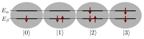
Figure 2: (color online) Schematic representation of the system under consideration. Four system states are considered depending on the relative occupation of the single-particle orbitals $|\alpha\rangle$ and $|\beta\rangle$, with energies $E_{\alpha}$ and $E_{\beta}$ respectively. Each orbital can in principle have different tunnel couplings to the leads.

IV.1 Population Probabilities

The occupation probabilities for the system to be in a given basis state are obtained from the diagonal elements of the RDM. We thus derive the algebraic system Eq. (5) for the $2$-channel system with states defined by Eq. (IV). The diagonal elements in Laplace space are given by,

$$\tilde{\rho}_{nn}(s)=\sum_{i,j,k,l}\left[\frac{G^{n}_{n}\left(1-\frac{1}{2}G^{i}_{j}G^{j}_{i}-\frac{1}{3}G^{i}_{i}G^{j}_{k}G^{k}_{i}\right)+G^{n}_{i}\left(G^{i}_{j}G^{j}_{j}+G^{i}_{j}G^{j}_{k}G^{k}_{k}-G^{k}_{j}G^{j}_{k}G^{i}_{i}\right)}{1-\frac{1}{2}G^{i}_{j}G^{j}_{i}-\frac{1}{3}\left(G^{i}_{j}G^{j}_{k}G^{k}_{i}+G^{i}_{j}G^{j}_{k}G^{k}_{l}G^{l}_{i}\right)+\frac{1}{8}G^{i}_{j}G^{j}_{i}G^{k}_{l}G^{l}_{k}}\right]\Xi_{ijkl}$$ (22)

where $\Xi_{ijkl}$ is the symmetric permutation tensor given by,

$$\Xi_{ijkl}=\begin{cases}1,&\text{$ijkl$ permutation of $0123$}\\ 0,&\text{otherwise}\end{cases},$$ (23)

and all indices run over the many-body system states defined in Eq. (IV).

In Eq. (22) the terms $G^{i}_{i}$ and $G^{i}_{j}$ are defined as

$$G^{i}_{i}=D^{-1}\left[~{}\tilde{\rho}_{i,i}(0)+\frac{\tilde{\rho}^{0}_{1,3}\tilde{R}_{i,i,1,3}(s)}{s+i\omega_{1,3}-\tilde{R}_{1,3,1,3}(s+i\omega_{1,3})}+\frac{\tilde{\rho}^{0}_{3,1}\tilde{R}_{i,i,3,1}(s)}{s+i\omega_{3,1}-\tilde{R}_{3,1,3,1}(s+i\omega_{3,1})}\right],$$ (24)

$$G^{i}_{j}=D^{-1}\left[~{}\tilde{R}_{i,i,j,j}(s)+\frac{\tilde{R}_{1,3,j,j}(s+i\omega_{1,3})\tilde{R}_{i,i,1,3}(s)}{s+i\omega_{1,3}-\tilde{R}_{1,3,1,3}(s+i\omega_{1,3})}+\frac{\tilde{R}_{3,1,j,j}(s+i\omega_{3,1})\tilde{R}_{i,i,3,1}(s)}{s+i\omega_{3,1}-\tilde{R}_{3,1,3,1}(s+i\omega_{3,1})}\right],$$

with,

$$D=s-\tilde{R}_{i,i,i,i}(s)-\frac{\tilde{R}_{1,3,i,i}(s+i\omega_{1,3})\tilde{R}_{i,i,1,3}(s)}{s+i\omega_{1,3}-\tilde{R}_{1,3,1,3}(s+i\omega_{1,3})}+\frac{\tilde{R}_{3,1,i,i}(s+i\omega_{3,1})\tilde{R}_{i,i,3,1}(s)}{s+i\omega_{3,1}-\tilde{R}_{3,1,3,1}(s+i\omega_{3,1})}.$$

In the Markov limit (Eq. (7)) the system of equations for the two-channel case is analytically solved in the time domain to obtain,

$$\rho(t)_{nn}=\frac{\sum_{nijk}P_{nijk}+\sum_{ijkq}P_{ijkq}\rho_{qq}(0)e^{-\sum_{pq}W_{pq}t}}{\sum_{ijkl}P_{ijkl}}$$ (25)

where, $P_{ijkl}=W_{ij}W_{jk}W_{kl}\Xi_{ijkl}$, with $\Xi_{ijkl}$ given by Eq. (23), and the transition rate $W_{ij}$ given by,

$$W_{ij} =\frac{2\pi}{\hbar^{2}}\sum_{r}\int_{-\infty}^{\infty}de_{\zeta}N_{r}|(T_{\zeta})_{r}|^{2}$$

$$\times\left[\delta\left(e_{\zeta}-\omega_{ij}\right)\Theta\left(\mu^{r}-e_{\zeta}\right)+\delta\left(\omega_{ij}-e_{\zeta}\right)\Theta\left(e_{\zeta}-\mu^{r}\right)\right].$$

where $r=\text{source},\text{drain}$, $\delta$ is the Dirac-delta function, and $\Theta$ is the Heaviside function.

As a case study to validate the non-Markovian approach, we analyze the effects of an orbital anisotropy on the dynamics of the system; we define edge and core system orbitals by the strength of their coupling to the reservoirs owing to the detailed shape of the wave function. Ciorga et al. (2002) In 2-dimensional parabolic confinement, for example, the particle’s wave function is composed of associated Laguerre polynomials where the core orbitals are weakly coupled to the leads owing to a poor ($s$-type) overlap with the reservoir states, whereas edge orbitals ($p$-type) are more strongly coupled to the reservoirs since these wavefunctions penetrate more deeply into the confining electrostatic barriers (see illustration Fig. 1b).

In relation to Fig. 2, we denote orbital $|\alpha\rangle$ an edge orbital and $|\beta\rangle$ a core orbital. Further denoting the orbital transmission by $T_{\alpha}$ and $T_{\beta}$, we can define an orbital anisotropy parameter as $\varepsilon=1-T_{\beta}/T_{\alpha}$, with $0<\varepsilon\leq 1$.

The following energy parameters are used in the subsequent analysis: applied bias $V_{\text{bias}}=6$ meV symmetric about the Fermi energy $\epsilon_{\text{Fermi}}=30$ meV, with two channels within the bias window, $E_{\alpha}=\epsilon_{\text{Fermi}}+1$ meV and $E_{\beta}=\epsilon_{\text{Fermi}}-1$ meV.

The non-Markovian system of Eq. (22), is evaluated numerically by performing an inverse Laplace transform as described in Sec. II, thus obtaining results for the diagonal elements of the RDM in the time domain.

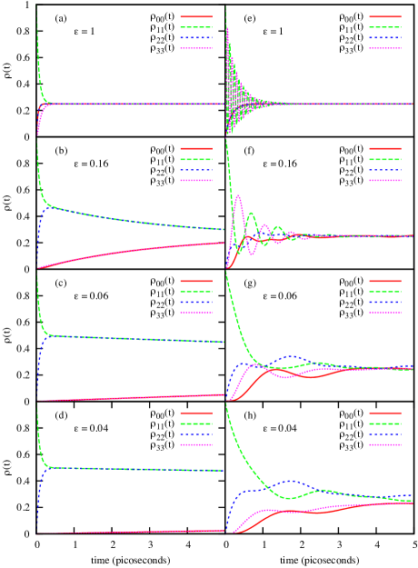
Figure 3: (color online) Markovian and non-Markovian time evolution of population probabilities in a quantum dot with 2 transport channels and four states. (See Fig. (2).) The plots are for symmetric source and drain tunnel barriers, and varying orbital asymmetry. We assume a $6$ meV bias symmetric about a $30$ meV Fermi energy, and two transport channels at energies $\epsilon_{\text{Fermi}}\pm 1$ meV. Plots (a) through (d) are results for the Markov limit (Eq. (7)), whereas plots (e) through (h) present results for the Non-Markovian theory.

The time evolution of the diagonal elements of the RDM in the large bandwidth limit are shown for increasing orbital anisotropy in Fig. 3. The set of figures on the left (Fig. 3.(a)-(d)) are the results obtained from the Markov limit by solving Eq. (7), while the figures on the right (Fig. 3.(e)-(h)) present the non-Markovian results based on Eq. (4). Four features in particular are evident in the non-Markovian results which we now discuss.

First, in the non-Markovian results, we observe high-frequency oscillations representing the coherent evolution of the occupancy between states with the same particle number, $|1\rangle$ and $|3\rangle$ (represented by RDM elements $\rho_{11}(t)$ and $\rho_{33}(t)$ see Eq. (IV)). As expected these oscillations are not present in the Markov limit.

Second, for small couplings to the core orbitals ($T_{\beta}\ll T_{\alpha}$) the four probabilities couple into two distinct pairs, states $|1\rangle$ and $|2\rangle$—the $N$ and $(N+1)$-particle ground states—are strongly coupled, as are states $|0\rangle$ and $|3\rangle$—the $(N-1)$-particle ground state and the $N$-particle first-excited state. We can understand why this occurs with recourse to Fig. 2. The transition between states $|1\rangle$ and $|2\rangle$ is through an edge orbital (with energy $E_{\alpha}$) and this coupling is stronger than the transition between $|1\rangle$ and $|0\rangle$ which involves a core orbital (with energy $E_{\beta}$). Similar arguments apply for the coupling between states $|3\rangle$ and $|0\rangle$ (strong coupling) and between $|3\rangle$ and $|2\rangle$ (weak coupling). This pairing of probability curves is also observed in the Markov limit, but again without oscillatory behaviour.

Third, in the steady state ($t\rightarrow\infty$), all occupation probabilities tend to the same value of 1/4. This is seen regardless of the tunnelling strengths of core and edge states as long as these rates are non-zero. The equal probability of 1/4 for each level can be understood as being due to the symmetric barriers between the dot and the source on the one hand, and between the dot and the drain on the other. Since these barriers are symmetric, any level will have an equal probability of being either occupied or unoccupied. Therefore in the steady state and under symmetric barriers the levels will be, on average, occupied and empty for the same amount of time. This result shows agreement with the Markov limit, where as expected all dynamical states would share equal probability in the steady state under symmetric barriers.

Fourth, although we observe that all four states are equally occupied in the steady state, the time to actually reach the steady states does depend on the relative couplings to the core and edge orbitals. As expected, we observe a disagreement with the Markov limit, where the Markovian results show that although the core or edge states probabilities couple at a much shorter time, the overall steady state is actually reached much later that in the non-Markovian results.

The fact that the time taken to reach the steady state increases as the tunnelling to the core state decreases can be understood as the effect of decreasing the available tunnelling pathways. Fewer pathways available means that the system takes longer to reach the steady state. This behaviour is exaggerated in the Markov approximation. In the limit of zero tunnelling to the core orbital, for example, states $|3\rangle$ and $|0\rangle$ will never become occupied, and the remaining two levels will each reach an occupation probability of $1/2$ rather than $1/4$, as expected by preservation of the trace. In this case the Markov limit agrees with the non-Markovian results.

Although much of the recent work in the area of non-equilibrium quantum dot systems has made use of Markovian-type approximations, Apalkov (2007); Imura et al. (2007); Pedersen et al. (2007); Egorova et al. (2003); Legel et al. (2007); Vaz and Kyriakidis (2008) it is fundamental to acknowledge the strict long-time limit requirement of these types of approximations in general, and thus their unreliability on the transient behavior of the system, mar especially when considering coherence properties of the system at short time scales. The disregard for the memory of the system in effect neglects most of the details of the coherent transient dynamics, and their use should only be invoked for coarse grained phenomena. Nonetheless, as expected, the Markov limit does yield reasonable results at sufficiently long times, Blum (1996); Suárez et al. (1992) when the system has reached a steady state, or when considering intermediate time scales of averaged behavior, such as the average total current through a system.

Figure 4: (color online) (a) Variation in the rate $\gamma$, of the decay of the oscillation of $\rho_{1,1}$. (b) Variation in the oscillation frequency of $\rho_{1,1}(t)$ as the orbital asymmetry is increased ($\varepsilon=1$ is maximum asymmetry).

Focusing now on the transient results shown in Fig. 3(e–h), we have extracted the positions and magnitudes of the peaks and fit fit these to a decaying exponential of the form $Ae^{-\gamma t}$. Results for the decay constant $\gamma$ for each value of $\varepsilon=1-T_{\text{core}}/T_{\text{edge}}$ are shown in Fig. 4(a). We observe a slower decay rate as the orbital asymmetry $(\varepsilon)$ is increased. We interpret this result by considering the change in relative occupation probability of the core channels relative to the edge channel as tunnelling to and from them is increasingly suppressed. In such a case the relative occupation of core states also decreases and any contribution from these states to the coherent evolution of the system will delay the overall decay to steady state, thus increasing the decoherence time.

In a similar manner we have extracted the frequency of oscillation as $\varepsilon$ is increased, where the results are shown in Fig. 4. The linear decrease of the frequency with an increase in $\varepsilon$ can be explained by again consider a decrease in the core channel’s occupation probability as $\varepsilon$ is increased. Therefore, a coherent superposition between states dependent on both core and edge channels will also exhibit the relative decrease in probability from the core-orbital state.

In the following section, we look at the coherence elements of the RDM under variations of the orbital anisotropy as well as of other relevant coupling and energetic parameters.

IV.2 Coherence

The evolution of the quantum coherence between system states with the same particle number, foc the Hilbert coherence, is coupled to the evolution of the occupation probabilities through the off-diagonal elements of the RDM. For the present 2-channel case, these coherence elements are derived in Laplace space to be,

$$\tilde{\rho}_{13}(s+i\omega_{13})=\frac{\tilde{\rho}^{0}_{13}+\sum_{n=0}^{3}\tilde{\rho}_{nn}(s)\tilde{R}_{13nn}(s+i\omega_{13})}{s+i\omega_{13}-\tilde{R}_{1313}(s+i\omega_{13})}$$ (26)

where the diagonal elements $\tilde{\rho}_{nn}(s)$ are given by Eq. (22), and $\omega_{13}$ is the energy difference between the $N$-particle states $|1\rangle$ and $|3\rangle$.

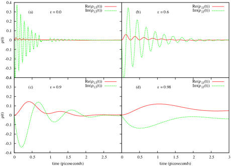
Figure 5: (color online) Time evolution of the real and imaginary parts of the off-diagonal elements of the RDM, $\rho_{13}(t)$, representing the Hilbert coherence of the system. The plots are for symmetric source and drain tunnel barriers, and varying orbital asymmetry. We assume a 6 meV bias symmetric about the Fermi energy, and two transport channels at energies $\epsilon_{\text{Fermi}}\pm 2$ meV. The coupling strength for the edge channel is set at $\hbar T_{\alpha(\text{edge})}=0.5meV$, while the coupling to the core channel is varied.

We numerically evaluate the Bromwich integral of Eq. (26) to obtain the real and imaginary parts of the off diagonal element $\tilde{\rho}_{13}(t)=\langle 1|\tilde{\rho}(t)|3\rangle$ in time-space. We are interested in the effects of the barriers and energy configuration of the system on the evolution of the coherence between dot states. In this regard, the important parameters considered are: 1) the orbital anisotropy, 2) the source/drain barrier asymmetry, 3) the thickness of the barriers (given inversely by the strength of the coupling $(T_{\alpha})_{r}$ between reservoir $r$ and dot orbital $\alpha$), 4) the energy level spacing $\Delta E$ between the transport channels present within the bias, 5) the applied bias voltage $V_{\text{bias}}$, and 6) the shift of energy levels within the bias window. The variations of these parameters are discussed below.

IV.2.1 Orbital Anisotropy

In Figure 5, we present results for the same energetics and variation in the orbital anisotropy as shown for the diagonal elements (Fig. 3). The Rabi-type coherent oscillations observed in Sec. IV.1 between the diagonal elements $\rho_{11}(t)$ and $\rho_{33}(t)$ are also clearly seen in the evolution of $\rho_{13}(t)$ as expected.

Investigating the effects of this orbital anisotropy on the evolution of the system, we focus on the decay constant and frequency of oscillation of the off-diagonal elements of the RDM as $(\varepsilon=1-T_{\text{core}}/T_{\text{edge}})$ is increased. In Fig. 6(a) the decay of the probability to a steady state is fitted fit by an exponential function with rate $\gamma$. We observe a slower decay rate as the orbital asymmetry factor $(\varepsilon)$ is increased. As in Sec. IV.1, we interpret this result by considering the change in relative occupation probability of states dependent on the core channel relative to states dependent on the edge channel, as tunnelling to and from the core channel is increasingly suppressed. In such a case the relative occupation of core states also decreases and any contribution from these states to the coherent evolution of the system will delay the overall decay to steady state, thus increasing the decoherence time.

The effect of a variation of the orbital anisotropy on the frequency of oscillation is shown in Fig. 6(b). We again observe a linear decrease of the frequency with an increase in $\varepsilon$. By the same argument as discussed in Sec. IV.1, we consider a decrease in the occupation probability of the core channel as $\epsilon$ is increased. A coherent superposition between states dependent on both the core and edge channels will also exhibit the relative decrease in probability from the core-dependent state. Thus as expected, the coherent evolution between states with the same particle number is described by the off-diagonal element $\rho_{13}(t)$.

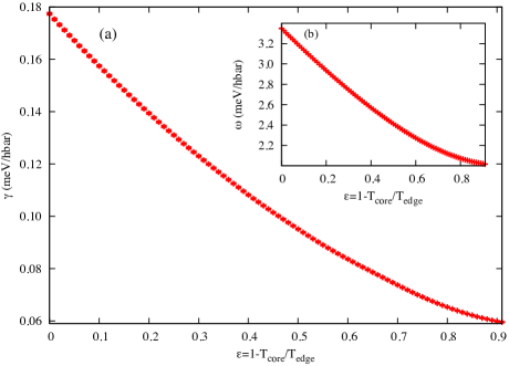
Figure 6: (color online) (a) Variation in the decay constant, $\gamma$, of the oscillation of $\rho_{13}(t)$, as the orbital asymmetry is increased ($\varepsilon=1$ is maximum asymmetry). (b) Inset, variation in the oscillating frequency of $\rho_{13}(t)$.

IV.2.2 Source/Drain Barrier Asymmetry

Keeping now the orbital anisotropy fixed and varying the asymmetry between the source and drain barriers, we observe that as the thickness of one barrier relative to the other is arbitrarily changed, there is a always an increase in the decay rate $\gamma$ (see Fig. 7a). This can be understood by considering the contribution to the decoherence rate due to various asymmetries: In the case where the drain barrier is thicker than the source barrier, tunnelling through the drain is suppressed relative to that through the source barrier. Therefore decoherence due to rapid tunnelling out of the dot is also suppressed. In the opposite case where the source barrier is thicker, tunnelling into the dot is suppressed relative to tunnelling out and thus, decoherence due to fast injection into the dot is also suppressed. Clearly, the decoherence will be greatest in the completely symmetric case since the contributions from both electron injection and extraction will be greatest.

Similarly, we find that the frequency of oscillation of the coherence term ($\rho_{13}(t)$) is also maximal in the completely symmetric case, and decreases otherwise (see Fig. 7b). This is expected since we can consider the frequency of oscillation to be proportional to the energy splitting due to the coupling with the reservoirs. Note that the shape of the curve in both the decay constant and frequency plots is quadratic with the relative thickness of the barrier. This is a consequence of the fact that, to leading order, dissipative effects are quadratic in the system-bath couplings. In the limit of infinitely thick barriers, there is no oscillation since tunnelling though the barrier has been completely suppressed.

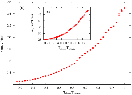
Figure 7: (color online) (a) Variation in the decay constant, $\gamma$, of the oscillation of the coherence element $\rho_{13}(t)$, as the asymmetry between the source and drain barriers is increased ($T_{\text{drain}}/T_{\text{source}}\neq 1$). (b) Inset, variation in the oscillating frequency of $\rho_{13}(t)$.

IV.2.3 Coupling Strength

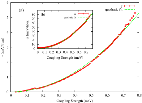
Figure 8: (color online) Variation of the decay $\gamma$ (a), and frequency of oscillation $\omega$ (b), as the overall coupling between orbitals and reservoirs is increased. The overall coupling is changed by varying the strength of the tunnelling rate $T_{\text{edge}}$ and by keeping a fixed orbital anisotropy of $\varepsilon=1-T_{\text{core}}/T_{\text{edge}}=0.3$

We now investigate the dependence of the coherence on the coupling strength between the reservoirs and the available orbitals in the dot while keeping the asymmetry between the barriers fixed. For simplicity, we also keep the ratio of the core-orbital tunneling rate to the edge orbital tunneling rate fixed such that the coupling strengths are varied at the same rate.

Figure 8 presents the change in the decay constant and the frequency of oscillation of the coherence element $\rho_{13}(t)$ as the coupling strength is varied. We observe that both the decay constant and frequency closely follow a quadratic fit on the coupling. As mentioned in the discussion of the results of barrier asymmetry, this is in agreement with the coupling effects being quadratic to leading order. We expect this to be a reasonable result in cases where sequential transport is the dominant process.

IV.2.4 Energy Level Spacing

Keeping now the barriers fixed, as well as the applied bias voltage, we look at a variation in the energy level spacing $\Delta E=E_{\alpha}-E_{\beta}$ between the $N$-particle states $|1\rangle$ and $|3\rangle$. (All previous results considered $\Delta E=2meV$.) Results for the decay constant and frequency are shown in figure 9(a) and (b), respectively. The level spacing is varied symmetrically about the Fermi energy. In this case we observe a decrease in the rate of decay as the level spacing is increased (Fig. 9a). This result can be understood in the following way: consider an electron in the source reservoir which tunnels into one of the available levels in the dot, and then tunnels out to the drain reservoir. Since the dot states are not eigenstates of the full Hamiltonian, the energy of the electron within the dot is not well defined and can have a value within the energy level spacing, $\Delta E$. As the electron tunnels from the source reservoir into the dot it can have at most an energy $E_{\text{max}}=\epsilon_{\text{Fermi}}+1/2eV_{\text{bias}}$. For the electron to then tunnel into a drain state, it must have an energy of at least $E_{\text{min}}=\epsilon_{\text{Fermi}}-1/2eV_{\text{bias}}+\Delta E$. Therefore, the available energy states of electrons that can tunnel into the dot from the source reservoir is given by $E_{\text{max}}-E_{\text{min}}=eV_{\text{bias}}-\Delta E$. Thus, the greater $\Delta E$ is, the fewer available energy states for transport into the dot, and the longer lived the dot states are. At approximately $1.5\ meV$ we observe a sudden drop in the decay constant leveling again after an increase in $\Delta E$ of  $0.5\ meV$. We investigate this feature by looking at its dependence on other parameters, and find that as the coupling strength between the reservoir and the dot is decreased, the feature decreases (see Fig. 9b). We also observe that the slope of the curve decreases after the drop, indicating a slower decrease of the decay constant.

The dependence of frequency of oscillation of the coherence on the energy level spacing is shown in Fig. 9b. The relevant energy differences giving rise to oscillations are the level spacing $\Delta E$ on the one hand, and the level energy and the edge of the bias window on the other. For small $\Delta E$, it is the latter which dominates and so $\omega$ shows weak dependence on $\Delta E$ as shown in Fig. 9b. For larger $\Delta E$, it is $\Delta E$ itself which dominates and so we see $\omega$ growing linearly with $\Delta E$.

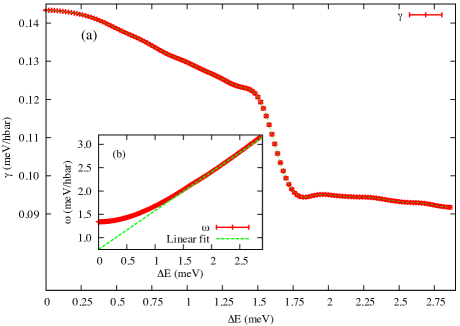
Figure 9: (color online) (a) Variation in the exponential decay constant $\gamma$, as the energy level spacing between the $|\alpha\rangle$ and $|\beta\rangle$ single particle levels is changed. Error bars indicate how well the decay is approximated as being exponential. (b) Variation in the frequency of coherent oscillation $\omega$ between many-body $N$-particle states $|1\rangle$ and $|3\rangle$.

IV.2.5 Applied Bias Voltage

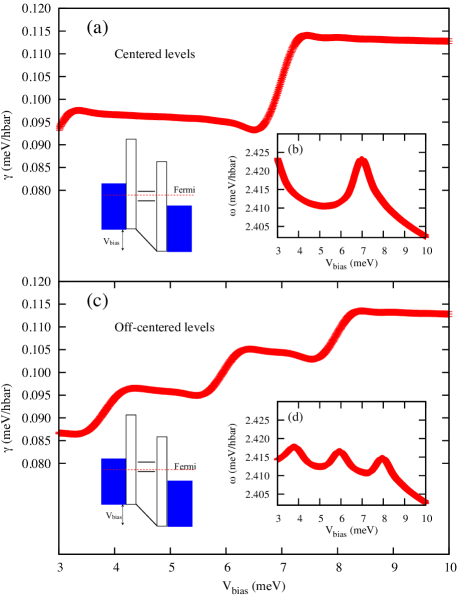
Figure 10: (color online) Variation of the decay constant $\gamma$ (a,c) and of the frequency of oscillation $\omega$ (b,d) as the applied bias voltage is increased symmetrically about the transport channels. In (a) and (b) the transport levels are kept symmetric about the center of the bias window, whereas in (c) and (d) the transport levels are shifted off-center within the bias window by $0.5meV$. In all cases, $\Delta E=2meV$.

A variation of the applied bias voltage has also been investigated, with the results presented in Fig. 10. Here $E_{\text{Fermi}}=30meV,E_{\alpha}=31meV,E_{\beta}=29meV$. For a symmetric variation of the bias voltage about the Fermi energy, we observe an overall increase of the decay constant as the bias voltage is increased (Fig. 10a). We explain this overall behaviour by considering that as the bias is increased, more energy states are available in the reservoirs for electrons to tunnel into or out of, electrons in the dot then have a larger number of tunneling pathways, thus increasing relaxations, and decoherence. This overall trend is also seen in the frequency of oscillation of the coherence (Fig. 10b) where, as the bias is increased, the frequency generally decreases. As discussed in Sec. IV.2.4, the frequency of oscillation follows the magnitude of the level spacing relative to the energy difference between the levels and the edge of the bias. Therefore, as the bias increases relative to the level spacing, the frequency of oscillation is expected to decrease.

Within this overall behaviour, we observe further structure in Fig. 10 in the form of pronounced plateaus occurring at specific intervals. This structure can be explained by noting that there are low frequency oscillatory envelopes (not shown) on the evolution of the RDM elements given by the interplay of all relevant energies in the system. The intervals from one plateau to the next are representative of the frequency of these slow envelope oscillations. The effect is also seen in the behaviour of the high frequency oscillations, where as the bias in increased, these form peaks with period given by the low frequency envelope (Fig. 10b).

We also find the number and position of these plateaus and peaks depends on the position of the levels within the bias window. Figures 10c and 10d show an increase in the number of plateaus as the levels inside the dot are shifted off-center by $0.1meV$ within the bias window ($E_{\alpha}=31.5meV,E_{\beta}=29.5meV$). Therefore the low frequency oscillations are strongly dependent on the relative energy difference between the level spacing and the spacing between the levels and the edge of the bias window.

Further analysis of these features will be the basis of future work by the authors.

IV.2.6 Energy Level Shift Within Bias Window

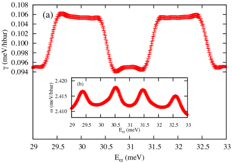
Figure 11: (color online) (a) Variation of the decay constant as the transport energy levels are shifted within the bias window. (b) Variation of the frequency of oscillation as the levels are shifted. Here $\Delta E=2meV$.

As mentioned in the discussion above, the position of the transport channels relative to the center of the bias window has consequences on the overall coherence between system states. As before, we keep the bias fixed at $6\ meV$ symmetric about a Fermi energy of $30\ meV$, giving a chemical potential for the source reservoir of $E_{\text{Fermi}}+\frac{1}{2}V_{\text{bias}}=33\ meV$. Similarly the chemical potential for the drain reservoir is then $E_{\text{Fermi}}-\frac{1}{2}V_{\text{bias}}=27\ meV$. By varying both levels simultaneously and keeping the level spacing at $\Delta E=2\ meV$, we can then move the edge level ($E_{\alpha}$) from $29\ meV$ to $33\ meV$ to sweep the levels over the entire window. Figure 11 presents the result of this shift of the position of $E_{\alpha}$. In a similar fashion to the variation of the applied bias, we observe structure in both the decay constant and frequency of oscillation of the coherence of the system. In Fig. 11a, the decay constant presents two plateaus nearly symmetrical about the Fermi energy with size in the order of $(0.5)\Delta E$. For the frequency of oscillation (Fig. 11b) we see that it presents peaks at about the same energies as the edges of the plateaus (similar to the results of variation of $V_{\text{bias}}$ in Fig. 10). We also observe an asymmetry of these peaks about the Fermi energy, where the overall height decreases as the levels increase past the center of the window. As discussed in Sec. IV.2.5, the plateaus appearing in the decay coefficient, and the peaks appearing in the frequency of oscillation are due to envelope oscillations of low frequency in the evolution of the RDM elements.

From these results, we can assert that the decoherence time is longest when the levels are either centered in the bias window, or with at least one level in resonance with the chemical potential of one of the reservoirs.

Similar to the results of Sec. IV.2.5, we cannot definitively ascribe a microscopic origin to these plateaus and peaks. Analysis of this structure will be the focus of future work.

IV.3 Summary

We now summarize the results of the variation of energy and coupling parameters on the decoherence and frequency of oscillations of the system. For the sequential transport model presented, the following conditions may independently increase the decoherence time in the system: An increase in the difference of tunnelling rates between available channels in the transport window, an increase in the barrier asymmetry between source and drain barriers, a decrease of the overall coupling strength between reservoirs and dot, an increase in the energy level spacing between available transport channels, a resonant case between available channels and reservoir Fermi energies or a relatively small bias voltage, a symmetrical positioning of transport levels within the bias window, or resonance between a transport level and a reservoir Fermi energy.

Similarly, the frequency of oscillation can be decreased by: An increase in the orbital anisotropy between available channels in the transport window, an increase in the barrier asymmetry between source and drain barriers, a decrease of the overall coupling strength between reservoirs and dot, a decrease in the energy level spacing between available transport channels, a resonant case between available channels and reservoir Fermi energies, a relatively high bias voltage, a symmetrical positioning of transport levels within the bias window. There is also the case that the frequency decreases in certain intervals as the bias voltage is increased or as positions of the energy levels are swept over the bias window. Table 1 presents a tabular summary of the above results.

Parameter	Decoherence-time	Frequency
Level Spacing	Increases	Increases
Bias voltage	Decreases	Decreases
Off-center shift	Decreases	Decreases
Coupling strength	Decreases	Increases
Barrier asymmetry	Increases	Decreases
Orbital anisotropy	Increases	Decreases

Table 1: Effects of increasing magnitude of parameters on coherence and frequency of oscillation.

We thus find that an optimal lifetime for the coherence between system states may be obtained by a suitable combination of the above energetic and interaction regimes. At the very least, by using the above criteria, it may be possible to confirm the barrier and energy parameters in experiment by studying decay rates and oscillatory behaviour.

V Concluding Remarks

We have developed a non-Markovian formalism for the transient evolution of the reduced density matrix of a quantum dot weakly coupled to source and drain reservoirs. Within a tunneling Hamiltonian approach, we have analytically derived an explicit memory kernel describing the sequential transport dynamics of the system for an arbitrary number of transport channels. The results of the analysis where compared with the Markov limit for a 2-channel (4-state) system, where we verified marked differences in the transient dynamics. Apart from the expected absence of coherent oscillatory behaviour in the Markovian results, it was also found that the rate at which the system approaches a steady state differs considerably between both theories in the regime of highly anisotropic tunneling into distinct system orbitals. It was found that the Markov approximation shows significantly longer time to reach a steady state when the tunnelling anisotropy is high, thus confirming its applicability only in the long-time limit. Through a comprehensive and systematic analysis, the decoherence time and frequency of oscillations observed in the non-Markovian results where found to depend on both the energy parameters of the system as well as the distinct coupling parameters to the reservoirs. Finally, distinct regimes have been outlined where both of these coherence characteristics could be increased.

VI Acknowledgements

This work is supported by Lockheed Martin Corporation and by the Natural Sciences and Engineering Research Council of Canada.

References

- Breuer and Petruccione (2002) H.-P. Breuer and F. Petruccione, The theory of open quantum systems (Oxford University Press, New York, 2002).
- Nakajima (1958) S. Nakajima, Prog. Theor. Phys 20, 948 (1958).
- Zwanzig (1960) R. Zwanzig, The Journal of Chemical Physics 33, 1338 (1960).
- Kraus (1971) K. Kraus, Ann. Phys. (N. Y.) 64, 311 (1971).
- Lindblad (1976) G. Lindblad, Commun. Math. Phys. 48, 119 (1976).
- Gorini et al. (1976) V. Gorini, A. Kossakowski, and E. Sudarshan, J. Math. Phys. 17, 821 (1976).
- Davies (1974) E. B. Davies, Commun. Math. Phys. 39, 91 (1974).
- Suárez et al. (1992) A. Suárez, R. Silbey, and I. Oppenheim, The Journal of Chemical Physics 97, 5101 (1992).
- Shah (1999) J. Shah, Ultrafast Spectroscopy of Semiconductors and Semiconductor Nanostructures (Springer, New York, 1999).
- (10) There are, however, some examples where an OQS does follow exact markovian dynamics, see for example Hepp and Liebb, Helv. Acta Phys. 46, 573 (1973) on the singular coupling limit, or Gurvitz and Prager, Phys. Rev. B 53, 15932 (1996) on quantum dots in the infinite bias regime.
- Braggio et al. (2006) A. Braggio, J. König, and R. Fazio, Physical Review Letters (2006).
- Bagrets et al. (2006) D. Bagrets, Y. Utsumi, D. Golubev, and G. Schön, Fortschritte der Physik (2006).
- Thielmann et al. (2005) A. Thielmann, M. Hettler, J. König, and G. Schön, Physical Review Letters (2005).
- Burkard (2009) G. Burkard, Physical Review B 79, 125317 (2009).
- Lee et al. (2004) J. Lee, I. Kim, D. Ahn, H. McAneney, and M. Kim, Physical Review A (2004).
- Coish and Loss (2004) W. A. Coish and D. Loss, Physical Review B 70 (2004).
- Knezevic (2008) I. Knezevic, Physical Review B 77, 18 (2008).
- Moldoveanu et al. (2009) V. Moldoveanu, A. Manolescu, and V. Gudmundsson, New Journal of Physics 11, 073019 (24pp) (2009).
- Kadanoff and Baym (1962) L. P. Kadanoff and G. Baym, Quantum Statistical Mechanics (W. A. Benjamin Inc, New York, 1962).
- Haug and Koch (1990) H. Haug and S. Koch, Quantum Theory of the Optical and Electronic Properties of Semiconductors (World Scientific, Singapore, 1990).
- Haug and Jauho (1996) H. Haug and A. P. Jauho, Quantum Kinetics in Transport and Optics of Semiconductors (Springer, Berlin, 1996).
- Wacker and Jauho (1998) A. Wacker and A. P. Jauho, Phys. Rev. Lett. 80, 369 (1998).
- Wacker et al. (1999) A. Wacker, A.-P. Jauho, S. Rott, A. Markus, P. Binder, and G. H. Döhler, Phys. Rev. Lett. 83, 836 (1999).
- Datta (1995) S. Datta, Electronic Transport in Mesoscopic Systems (Cambridge University Press, Cambridge, 1995).
- Datta (2000) S. Datta, Superlattices Microstruct. 28, 253 (2000).
- Knezevic and Ferry (2003) I. Knezevic and D. Ferry, Phys. Rev. E 67, 066122 (2003).
- Alicki and Lendi (2007) R. Alicki and K. Lendi, Lecture notes in Physics: Recent Developments (2007).
- Gardiner and Zoller (2004) C. W. Gardiner and P. Zoller, Quantum Noise: A Handbook of Markovian and Non-Markovian Quantum Stochastic Methods with Applications to Quantum Optics (Springer, Berlin, 2004).
- Blum (1996) K. Blum, Density Matrix Theory and Applications (Springer, New York, 1996).
- (30) This condition can be directly obtained from the normalization condition , and the mixed-state condition .
- Knezevic and Ferry (2002) I. Knezevic and D. K. Ferry, Physical Review E 66 (2002).
- Abramowitz and Stegun (1964) M. Abramowitz and I. A. Stegun, Handbook of Mathematical Functions with Formulas, Graphs, and Mathematical Tables (Dover, New York, 1964).
- (33) The Bromwich integral is evaluated using an adaptive Fourier integration routine using tables of Chebyshev moments. See, for example, the qawf algorithms in the GNU scientific library (http://www.gnu.org/software/gsl).
- Mahan (1981) G. D. Mahan, Many-particle Physics (Plenum, New York, 1981).
- Kouwenhoven et al. (2001) L. P. Kouwenhoven, D. G. Austing, and S. Tarucha, Reports on Progress in Physics 64, 701 (2001).
- Chen et al. (2009) J. C. Chen, M.-Y. Li, T. Ueda, and S. Komiyama, Applied Physics Letters 94, 232109 (2009).
- Ciorga et al. (2002) M. Ciorga, A. Wensauer, M. Pioro-Ladriere, M. Korkusinski, J. Kyriakidis, A. S. Sachrajda, and P. Hawrylak, Phys. Rev. Lett. 88, 256804 (2002).
- Apalkov (2007) V. M. Apalkov, Phys. Rev. B 75, 5 (2007).
- Imura et al. (2007) K. Imura, Y. Utsumi, and T. Martin, Physical Review B 75, 205341 (2007).
- Pedersen et al. (2007) J. N. Pedersen, B. Lassen, A. Wacker, and M. H. Hettler, Phys. Rev. B 75, 235314 (2007).
- Egorova et al. (2003) D. Egorova, M. Thoss, W. Domcke, and H. Wang, J. Chem. Phys. 119, 2761 (2003).
- Legel et al. (2007) S. Legel, J. König, G. Burkard, and G. Schön, Phys. Rev. B 76, 085335 (2007).
- Vaz and Kyriakidis (2008) E. Vaz and J. Kyriakidis, J. Chem. Phys. 129, 024703 (2008).
- (44) Our fit was performed using an implementation of the nonlinear least-squares Marquardt-Levenberg algorithm, where the error bars are calculated from the variance of the residuals.
- (45) An analysis of a Fock-space coherence among states with differing particle numbers in underway by the authors.