Ordered states of adatoms on graphene.

Abstract

We show that a dilute ensemble of epoxy-bonded adatoms on graphene has a tendency to form a spatially correlated state accompanied by a gap in graphene’s electron spectrum. This effect emerges from the electron-mediated interaction between adatoms with a peculiar $1/r^{3}$ distance dependence. The partial ordering transition is described by a random bond three state Potts model.

Graphene (monolayer of graphite) is a truly two-dimensional crystal, just one-atom-thick Geim1 . It is a gapless semiconductor with charge carriers mimicking relativistic dynamics of massless Dirac fermions Review , a peculiarity dictated by the bonding of carbon atoms into a highly symmetric honeycomb lattice. Graphene can host various adsorbents, in particular atoms, retaining its own structural integrity. Such chemisorbed atoms (adatoms) may strongly affect electronic properties of graphene Geim3 ; Fuhrer ; Lanzara ; Geim2 introducing symmetry-breaking perturbations into the lattice. The type of symmetry breaking depends on the position of the adatom in the hexagonal unit cell of the crystal. In particular, alkali atoms position themselves over the centres of the hexagons K . Oxygen, nitrogen, boron, or an additional carbon C-on-G prefer ’epoxy’ bonded positions (e-type) and reside above the middle of a carbon-carbon bond. Atomic hydrogen and halogens reside in the symmetric on-site position above the carbon (s-type) H-on-G . It has also been noticed that a pair of hydrogen atoms on the neighbouring sites of graphene lattice forms a stable H-H dimer which acts as an e-type adsorbent H2-on-G .

Here we predict that an ensemble of e-type adatoms (those perturbing C-C bonds) tend to order, mimicking a superlattice structure, even when graphene coverage by adsorbents is low. The underlying mechanism is a long-range electron-mediated interaction between adatoms similar to the RKKY exchange between localized spins in metals RKKY1954 . The effect is peculiar to graphene. Unlike metals, charge neutral graphene has a point-like Fermi surface positioned in the corners $\mathbf{K}$ and $\mathbf{K}^{\prime}=-\mathbf{K}$ of the hexagonal Brillouin zone – called valleys. The electron density of states vanishes at the Fermi level. As a result, the Friedel oscillations in charge neutral graphene are commensurate with its honeycomb lattice and decay as the inverse cube of the distance to the adatom Fertig . We show that such an interaction in a dilute ensemble of e-type adsorbents may result in their partial ordering associated with a superlattice structure with the unit cell three times larger than in graphene, as illustrated in Fig. 1. We present our results in the following order. Starting with a particular tight-binding model for an e-type adsorbent, we determine the form of a perturbation it creates for the electrons in graphene. Using group theory we classify such interactions beyond a specific microscopic model and determine the conditions under which RKKY interaction between adatoms leads to a partially ordered state with a gapful electronic spectrum. We conclude by discussing experimental signatures of the effect.

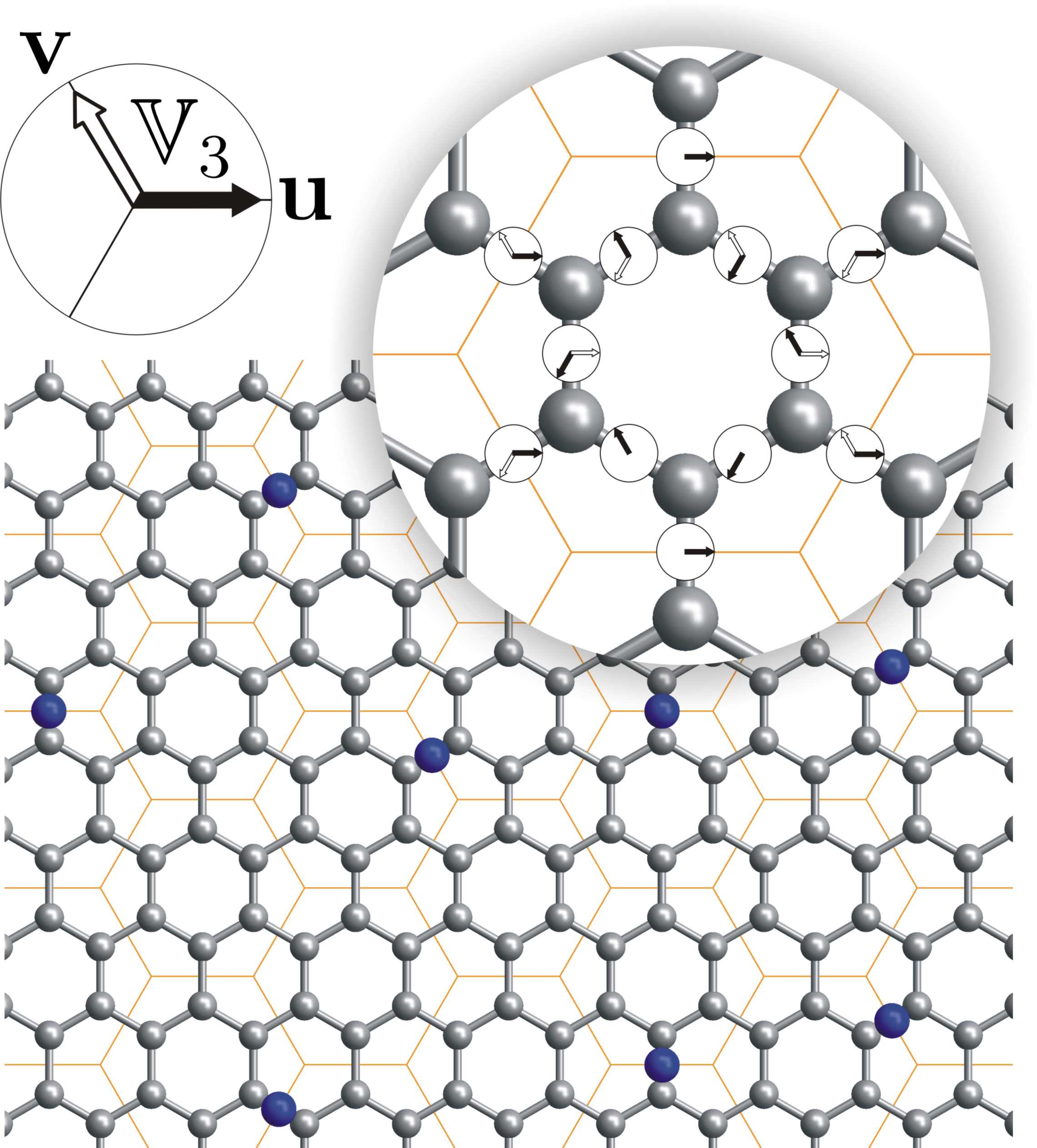
Figure 1: An ordered ensemble of adatoms (blue) on graphene lattice: all impurity atoms occupy positions at the intersection of graphene bonds and the bonds of the underlying fictitious superlattice. The inset shows how the superlattice originates from the scattering matrix $\hat{W},$ Eq. (3). To each bond there corresponds a pair of vectors $(\mathbf{u},\mathbf{v})$ forming a periodic pattern with three times graphene lattice’s period.

Table 1: Symmetry-based classification of RKKY interactions for different types of adatoms. The parameterization of the adatom scattering matrix $\hat{W}_{a}$ is given in terms of an orbit $\mathcal{W}_{i}$ of the lattice symmetry group in a given irrep $i.$ The potential $\Omega_{ab}^{(i)},$ is a contribution of the given orbit to the adatom-adatom interaction, Eqs. (5). The last column indicates ordering favored by the given interaction term.

Irrep $i$	Orbit $\mathcal{W}_{i}$	$\Omega_{ab}^{(i)}$	type: position	Partial order
$A_{1}$	$\mathbbm{1}$	$-1/2$	All	—
$B_{2}$	$s\Sigma_{z}\Lambda_{z}$, $s=\pm 1$	$s_{a}s_{b}$	s: units ¡0.08 pt,0.08 pt¿ x from -130 to 130, y from -180 to 180 =.2pt 2 pt (.) 0 100 87 50 / 87 50 87 -50 / 87 -50 0 -100 / 0 -100 -87 -50 / -87 -50 -87 50 / -87 50 0 100 / 0 100 0 150 / 87 50 130 75 / 87 -50 130 -75 / 0 -100 0 -150 / -87 -50 -130 -75 / -87 50 -130 75 /	Sublattice
$E_{1}^{\prime}$	$\Sigma_{z}\mathbf{(}\mathbf{\Lambda}\cdot\mathbf{u})$, $\mathbf{u}\in\mathbb{V}_{3}$	$\mathbf{u}_{a}\cdot\mathbf{u}_{b}$	e: units ¡0.08 pt,0.08 pt¿ x from -130 to 130, y from -180 to 180 =.2pt 2 pt (.) 0 100 87 50 / 87 50 87 -50 / 87 -50 0 -100 / 0 -100 -87 -50 / -87 -50 -87 50 / -87 50 0 100 / 0 100 0 150 / 87 50 130 75 / 87 -50 130 -75 / 0 -100 0 -150 / -87 -50 -130 -75 / -87 50 -130 75 /	$3\times$ unit cell superlattice
$E_{2}$	$\Lambda_{z}\mathbf{(}\mathbf{\Sigma}\cdot\mathbf{v})$, $\mathbf{v}\in\mathbb{V}_{3}$	$\mathbf{v}_{a}\cdot\mathbf{v}_{b}-\frac{3}{2}(\mathbf{n}\cdot\mathbf{v}_{a})(\mathbf{n}\cdot\mathbf{v}_{b})$	e: units ¡0.08 pt,0.08 pt¿ x from -130 to 130, y from -180 to 180 =.2pt 2 pt (.) 0 100 87 50 / 87 50 87 -50 / 87 -50 0 -100 / 0 -100 -87 -50 / -87 -50 -87 50 / -87 50 0 100 / 0 100 0 150 / 87 50 130 75 / 87 -50 130 -75 / 0 -100 0 -150 / -87 -50 -130 -75 / -87 50 -130 75 /	None
$G$	$(\mathbf{v}\times\mathbf{\Sigma})(\mathbf{u}\times\mathbf{\Lambda})$, $\mathbf{u},\mathbf{v}\in\mathbb{V}_{3}$	$\frac{1}{2}(\mathbf{u}_{a}\cdot\mathbf{u}_{b})[3(\mathbf{n}\cdot\mathbf{v}_{a})(\mathbf{n}\cdot\mathbf{v}_{b})-(\mathbf{v}_{a}\cdot\mathbf{v}_{b})]$	e: units ¡0.08 pt,0.08 pt¿ x from -130 to 130, y from -180 to 180 =.2pt 2 pt (.) 0 100 87 50 / 87 50 87 -50 / 87 -50 0 -100 / 0 -100 -87 -50 / -87 -50 -87 50 / -87 50 0 100 / 0 100 0 150 / 87 50 130 75 / 87 -50 130 -75 / 0 -100 0 -150 / -87 -50 -130 -75 / -87 50 -130 75 /	None
$E_{1}^{\prime\prime}$	$\begin{array}[]{l}s\Sigma_{x}(\bm{\Lambda}\cdot\hat{s}\mathbf{u})+\Sigma_{y}(\bm{\Lambda}\times\hat{s}\mathbf{u})\\ \hat{s}=\mathrm{diag}(1,s)\end{array}$, $\begin{array}[]{l}\mathbf{u}\in\mathbb{V}_{3},\\ s=\pm 1\end{array}$	$\frac{2-s_{a}s_{b}}{2}\left[(\mathbf{n}\cdot\mathbf{u}_{a})(\mathbf{n}\cdot\mathbf{u}_{b})-s_{a}s_{b}(\mathbf{n}\times\mathbf{u}_{a})(\mathbf{n}\times\mathbf{u}_{b})\right]$	s: units ¡0.08 pt,0.08 pt¿ x from -130 to 130, y from -180 to 180 =.2pt 2 pt (.) 0 100 87 50 / 87 50 87 -50 / 87 -50 0 -100 / 0 -100 -87 -50 / -87 -50 -87 50 / -87 50 0 100 / 0 100 0 150 / 87 50 130 75 / 87 -50 130 -75 / 0 -100 0 -150 / -87 -50 -130 -75 / -87 50 -130 75 /	None

The $\pi$-electron band in graphene is well described by the closest-neighbor tight-binding model, $H_{0}=\gamma_{0}\sum_{[\mathbf{r}_{A}\mathbf{r}_{B}]}\{c_{\mathbf{r}_{A}}^{\dagger}c_{\mathbf{r}_{B}}+h.c.\}$ with hoping parameter $\gamma_{0}\sim 3\text{eV}$ Review . The sum runs over all pairs $[\mathbf{r}_{A}\mathbf{r}_{B}]$ of neighboring A and B sites of the lattice and $c^{\dagger}$/$c$ are the on-site electron creation/annihilation operators footnoteSpin . An e-type adatom attached to the bond between the cites $\mathbf{r}_{A}^{\prime}$ and $\mathbf{r}_{B}^{\prime}$ creates a local perturbation

$$H_{a}=\gamma_{0}\xi_{1}(c_{\mathbf{r}_{A}^{\prime}}^{\dagger}c_{\mathbf{r}_{A}^{\prime}}+c_{\mathbf{r}_{B}^{\prime}}^{\dagger}c_{\mathbf{r}_{B}^{\prime}})+\gamma_{0}\xi_{2}(c_{\mathbf{r}_{A}^{\prime}}^{\dagger}c_{\mathbf{r}_{B}^{\prime}}+c_{\mathbf{r}_{B}^{\prime}}^{\dagger}c_{\mathbf{r}_{A}^{\prime}}),$$ (1)

where $\xi_{1},\xi_{2}<1$ determine how the adatom affects the on-cite potential ($\xi_{1}$) and the electron hopping amplitude between the cites ($\xi_{2}$).

The long-range RKKY interaction between two adatoms is due to the perturbation of the electron spectrum near the Fermi energy and is adequately described in terms of the four-component field, $\psi(\mathbf{r})=(\psi_{1},\psi_{2},\psi_{3},\psi_{4})^{T}$, which is smooth on a scale of the lattice constant, $a$:

$$c_{\mathbf{r}}=\left(\textstyle\frac{3}{4}\right)^{\frac{1}{4}}a\times\left\{\begin{array}[]{ll}e^{i\mathbf{K}\mathbf{r}}\psi_{1}(\mathbf{r})+e^{-i\mathbf{K}\mathbf{r}}\psi_{4}(\mathbf{r}),&\quad\mathbf{r}=\mathbf{r}_{A}\\ e^{i\mathbf{K}\mathbf{r}}\psi_{2}(\mathbf{r})+e^{-i\mathbf{K}\mathbf{r}}\psi_{3}(\mathbf{r}),&\quad\mathbf{r}=\mathbf{r}_{B}\end{array}\right..$$

In the presence of an adatom $\psi(\mathbf{r})$ obeys the Hamiltonian Impurities

$$\hat{H} =v\int\psi^{\dagger}(\mathbf{\Sigma}\cdot\mathbf{\hat{p}})\psi d^{2}r+\hbar va\psi^{\dagger}(\mathbf{r}_{a})\hat{W}_{a}\psi(\mathbf{r}_{a}),$$ (2)

$$\hat{W}_{a} =\lambda_{A_{1}}+\lambda_{E_{1}^{\prime}}\Sigma_{z}(\mathbf{\Lambda}\cdot\mathbf{u}_{a})$$

$$\quad+\lambda_{E_{2}}\Lambda_{z}(\mathbf{\Sigma}\cdot\mathbf{v}_{a})+\lambda_{G}(\mathbf{\Lambda}\times\mathbf{u}_{a})\cdot(\mathbf{\Sigma}\times\mathbf{v}_{a}),$$ (3)

with $v=\sqrt{3}a\gamma_{0}/2\hbar$ and $\Sigma_{x,y}=\sigma_{x,y}^{\mathrm{s}}\otimes\sigma_{z}^{\mathrm{v}}.$ The Pauli matrices $\sigma_{x}^{\alpha},\sigma_{y}^{\alpha}$ and $\sigma_{z}^{\alpha}$ operate on the valley ($\alpha=\mathrm{v}$) or sublattice ($\alpha=\mathrm{s}$) indices. Together with $\Sigma_{z}=\sigma_{z}^{\mathrm{s}}\otimes\mathbf{1}^{\mathrm{v}}$, matrices $\Sigma_{x,y}$ form a representation of the $\mathrm{SU}_{2}^{\Sigma}$ algebra. The first term in $H$ determines the Dirac electronic spectrum. It possesses a ”flavour” $\mathrm{SU}_{2}^{\Lambda}$ symmetry generated by the three matrices $\Lambda_{x,y}=\sigma_{z}^{\mathrm{s}}\otimes\sigma_{x,y}^{\mathrm{v}}$ and $\Lambda_{z}=\mathbf{1}^{\mathrm{s}}\otimes\sigma_{z}^{\mathrm{v}}$, satisfying $[\Lambda_{i},\Sigma_{j}]=0$. This symmetry manifests of the conservation of the electron’s valley index. Matrices $\Sigma$, $\Lambda$ and their products $\Lambda_{i}\Sigma_{j}$ can be arranged into irreducible representations (irreps) of the symmetry group $\mathcal{G}$ of the honeycomb lattice Kechedzhi ; Basko , which includes lattice translations, $C_{6v}$ rotations and mirror refections. All operators $\Sigma_{i}$ and $\Lambda_{j}$ change signs upon time inversion, therefore only products $\Lambda_{i}\Sigma_{j}$ are time-inversion-symmetric and can appear in the scattering matrix footnoteT $\hat{W}_{a}$ , Eq. (2), describing static perturbations DisorderedG ; FO created by adatoms.

For an adatom of a general symmetry type $\hat{W}_{a},$ can be expanded into orbits in the irreps footnoteG of $\mathcal{G},$ $\hat{W}_{a}=\sum\lambda_{i}\mathcal{W}_{i}$. The classification of orbits by the irrep and the symmetry type of adatom is given in the second column of Table 1. In particular, the matrix $\hat{W}_{a}$ of an e-type adatom (or the H-H dimer) is expanded into orbits in the irreps $A_{1},E_{1}^{\prime},E_{2}$ and $G,$ corresponding to the four terms in Eq. (3). Vectors $\mathbf{u}$ and $\mathbf{v}$ in Eq. (3) take values in the set $\mathbb{V}_{3}$ shown in Fig. 1: three unit vectors on the x-y plane, at $120^{\circ}$ angles. Each given bond of graphene lattice is characterized by a pair $(\mathbf{u},\mathbf{v)}$ as shown in Fig. 1. The distribution of $\mathbf{u}$ and $\mathbf{v}$ forms a periodic pattern with three times the graphene lattice period: the intervalley scattering implies the momentum transfer $\Delta\mathbf{K}=\mathbf{K}-\mathbf{K}^{\prime}$ such that $3\Delta\mathbf{K}$ is a reciprocal lattice vector. Thus, $\hat{W}_{a}$ in the e-type case is periodic on a superlattice, whose unit cell is three times as big as graphene’s and contains nine distinguishable C-C bonds. The three non-trivial terms in Eq. (3) resemble the coupling of an electron to the in-plane $\Gamma$- and K-point phonons Basko . Indeed, the $E_{1}^{\prime}$ term parameterized by the vector $\mathbf{u}$ resembles the effect of the K-point breathing phonon mode. Below, the ensemble average of $\mathbf{u}$ will play the role of the order parameter. The $G$ term is similar to the 4-fold degenerate K-point lattice mode. The $E_{2}$ term resembles the uniaxial strain due to a $\Gamma$-point optical phonon. The parameters $\lambda_{i}$ in $\hat{W}_{a}$ are specific for particular atoms. For the model in Eq. (1), $\lambda_{E_{1}^{\prime}}=\lambda_{E_{2}}=\xi_{2}$ and $\lambda_{A_{1}}=\lambda_{G}=\xi_{1}$.

Unlike e-type adatoms, the perturbation introduced by an s-type adatom (e.g., H on a lattice site) cannot be related to the in-plane phonons, since it explicitly distinguishes A and B sublattices of graphene. The two orbits encountered in the matrix $\hat{W}_{a}$ in this case can be related to the out-of-plane phonons in the presence of a transverse electric field ($z\rightarrow-z$ asymmetry): $B_{1}$ resembling the $\Gamma$-point and $E_{1}^{\prime\prime}$ the K-point phonon. In both cases, the A/B-residency of an adatom is accounted for by $s=\pm 1$.

Each type of the adsorbents listed in Table 1 creates Friedel oscillations of the electron density breaking the symmetry in the same way as the adatom does. The polarization caused by one adatom extends over long distances, thus leading to interaction between the adatoms. The energy of this interaction between a pair of adatoms at a distance $|\mathbf{r}_{ab}|\gg a$ can be expressed through the imaginary time (Matsubara) Green function of electrons in a clean graphene, $G(\mathbf{r},\tau)$ footnoteGmom as

$$F {}_{ab}=2\hbar v^{2}a^{2}\mathrm{Tr}\int_{-\infty}^{\infty}d\tau\hat{W}_{a}\hat{G}(\mathbf{r}_{ab},\tau)\hat{W}_{b}\hat{G}(-\mathbf{r}_{ab},-\tau),$$

$$\hat{G} (\mathbf{r},\tau)=-\frac{1}{4\pi}\frac{v\tau+i\mathbf{\Sigma}\cdot\mathbf{r}}{(v^{2}\tau^{2}+r^{2})^{3/2}}.$$ (4)

Here, trace is taken over the valley and sublattice indices, and spin degeneracy is taken into account. Equation (4) yields a long-range pair correlation energy,

$$F_{ab} = -\frac{\hbar va^{2}}{4\pi}\frac{\Omega_{ab}}{r_{ab}^{3}},\qquad\mathbf{n}=\frac{\mathbf{r}_{ab}}{r_{ab}},$$

$$\Omega_{ab} = \frac{1}{16}\mathrm{\ Tr}\left[\;\hat{W}_{b}\hat{W}_{a}-3\hat{W}_{a}(\mathbf{\Sigma}\cdot\mathbf{n})\hat{W}_{b}(\mathbf{\Sigma}\cdot\mathbf{n})\right].$$ (5)

Interaction between adatoms of the same type depends on both the type of the adatoms and the parameters $\lambda_{i}$ characterizing the adatom-electron coupling in each symmetry-breaking interaction channel $\mathcal{W}_{i}$:

$$\Omega_{ab}=\sum_{i}\lambda_{i}^{2}\Omega_{ab}^{(i)}.$$ (6)

For the model in Eq. (3) with $\lambda_{E_{1}^{\prime}}$ larger than other coupling parameters, $\Omega_{ab}\approx\lambda_{E_{1}^{\prime}}^{2}\mathbf{u}_{a}\cdot\mathbf{u}_{b}$, so that the interaction between lateral degrees of freedom of the two adsorbents looks like an isotropic ferromagnetic exchange. Therefore the adatoms tend to occupy preferably bonds with the same $\mathbf{u}$ and form a partially ordered state shown in Fig. 1. The transition to such a state is described by a special case of random exchange three-state Potts model Wu : ’spins’ $\mathbf{u}$ reside on randomly distributed with density $\rho$ sites and experience pairwise exchange interaction $-J\mathbf{u}_{a}\cdot\mathbf{u}_{b}/r^{3}.$ According to recent cluster Monte-CarloUs studies this model undergoes an order-disorder transition at a critical temperature $T_{c}\approx 8\rho^{3/2}J.$ For the Eq. (1) model $T_{c}$ is evaluated as

$$T_{c}\approx 0.6\lambda_{E_{1}^{\prime}}^{2}(a^{2}\rho)^{3/2}\frac{{\hbar v}}{a}.$$ (7)

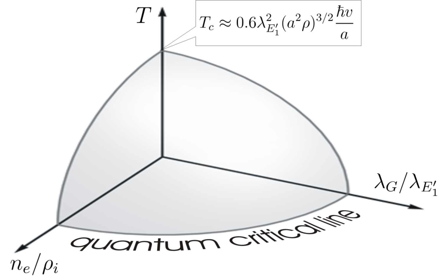
Figure 2: The schematic phase diagram of the epoxy-bonded adatom system on graphene. The critical surface separates the gapped ordered phase (Fig. 1) from the disordered phase.

Consider now effects of other terms in (6) allowed by the e-type symmetry. These terms are listed in the rows $A_{1}$, $E_{2}$ and $G$ in Table 1. The symmetric perturbation parameterized by $\lambda_{A_{1}}$ leads to the repulsion between adatoms regardless of which bonds of the extended supercell they occupy. The coupling parameterized by $\lambda_{E_{2}}$ causes an anisotropic ’antiferromagnetic’ interaction of the alternative set of Potts ”spins” $\mathbf{v}_{a}$. Frustration precludes ordering of $\mathbf{v}_{a},$ which could lead to a unilateral deformation of the lattice. However, a presence of $\lambda_{E_{2}}^{2}\Omega_{ab}^{(E_{2})}$ in $\Omega_{ab},$ Eq. (6) does not affect the ordering of vectors $\mathbf{u}_{a},$ at least up to the quadratic order in $\lambda_{E_{2}}.$ The isotropic interaction leading to the ordering only competes with the anisotropic interaction between adatoms caused by the last term in $\hat{W}_{a}$, Eq. (3) (the fifth row of Table 1). If the latter is strong, $\lambda_{G}>\lambda_{E_{1}^{\prime}}$, it suppresses ordering by frustration. As a result, $T_{c}$ of the order-disorder transition decreases with increasing ratio $\lambda_{G}/\lambda_{E_{1}^{\prime}}$ until it vanishes at a quantum critical point.

Increasing the density $n_{e}$ of mobile carriers in graphene should also suppress $T_{c}.$ Indeed, at finite $n_{e}$ the RKKY interaction develops Friedel oscillationsFO , $F\propto(\mathbf{u}_{a}\cdot\mathbf{u}_{b})\sin^{2}(k_{F}r)/r^{2},$ which lead to a random sign of the exchange coupling between adatoms at distance $r_{ab}>\sqrt{1/n_{e}}.$ At sufficiently large ratio $n_{e}/\rho$ this effect should completely destroy ordering of Potts ”spins”. These considerations are illustrated by the phase diagram in Fig. 2, where the ”quantum critical line” corresponds to the parametric condition $T_{c}(n_{e}/\rho,\lambda_{G}/\lambda_{E^{\prime}})\to 0.$ Further analysis of these transitions is beyond the scope of this paper.

The interaction of s-type adsorbents residing on the honeycomb lattice sites (e.g., hydrogen) is described in rows 2 and 6 of Table 1. Each s-type adatom can be characterized by the Ising ”spin” $s_{a}$ taking the value $+1$ or $-1$ depending on which sublattice A or B it occupies. These spins may, potentially, establish sublattice ordering. However, there will be no ordering of the ”spins” $\mathbf{u}_{a}:$ the interaction described in Table 1 is anisotropic and causes frustrations. In contrast, a pair of hydrogens forming an H-H dimer on the nearest A/B sites H2-on-G falls into the same symmetry class as e-type adatoms and can establish the same type of ordering. It has been noticed that in hydrogenated graphite both configurations of H atoms are present H2-on-G . Since the decomposition of the interaction in Eq. (5) suggests the absence of mutual correlations between adsorbents of the e-type and s-type, we expect ordering of the H-H dimers on graphene, even if only a fraction of hydrogens covering the flake is dimerised.

The predicted ordering will strongly influence transport and optical properties of the material. As temperature approaches $T_{c}$ from above large clusters of ordered phase will act as intervalley-scattering Bragg mirrors for electrons. Back-scattering from such mirrors should lead to a power-law increase of resistivity near $T_{c}$ TBP . At $T<T_{c}$, the spectrum of electrons becomes gapful,

$$\varepsilon=\pm\sqrt{v^{2}p^{2}+\Delta^{2}},\;\;\Delta=\frac{\hbar v}{a}\lambda_{E_{1}^{\prime}}\rho a^{2}\gg T_{c},$$ (8)

as can be seen from the mean-field Hamiltonian Kekule1 , $\langle\hat{H}\rangle=v\mathbf{\Sigma}\cdot\mathbf{p}+\hbar v\rho a\lambda_{E_{1}^{\prime}}\Sigma_{z}\mathbf{\Lambda}\cdot\mathbf{u,}$ valid for $p\ll\hbar\rho^{1/2}$. At low carrier density this will lead to the activated transport regime typical of semiconductors.

Partial ordering of e-type adsorbents should also be manifest in the structure of the D-peak in the Raman spectrum. The D-peak is associated with the excitation of one optical phonon at momentum $\mathbf{K}$ (or $\mathbf{K}^{\prime}$) and is forbidden by momentum conservation in pristine graphene. In the presence of random scatterers, the D-peak is seen as a low-intensity, $I(T>T_{c})\propto\rho\lambda_{E_{1}^{\prime}}^{2},$ feature strongly broadened due to the disorder-induced uncertainty in the emitted phonon momentum. Domains of ordered adsorbent, with the size $L$, will scatter electrons between valleys $K$ and $K^{\prime}$ coherently. This will enhance the intensity of the otherwise forbidden transition, $I(T<T_{c})\propto\rho\lambda_{E_{1}^{\prime}}^{2}\times\rho L^{2}\gg g(T>T_{c})$, and restrict the uncertainty of the emitted phonon momentum to $\delta q\sim 1/L$. Thus, one can predict that the ordering of adatoms abruptly enhances and narrows the D-peak in the Raman spectrum. To mention, an observation of a hopping conductivity accompanied by a sharp high-intensity D-line in the Raman spectrum in graphene exposed for a long time to hydrogen atmosphere has been reported in Ref. Geim2 . We predict a similar behavior of the ARPES spectrum of graphene: ordering should strongly enhance the photoemission of electrons from the center of the Brillouin zone at energies close to the Fermi energy.

The work was supported by the Lancaster-EPSRC Portfolio Partnership, ESF CRP SpiCo, and US DOE contract No. DE-AC02-06CH11357.

References

- (1) K.S. Novoselov, et al, Science 306, 666 (2004).
- (2) A.H. Castro Neto, et al, Rev. Mod. Phys. 81 , 109 (2009).
- (3) F. Schedin, et al, Nature Materials 6, 652-655 (2007).
- (4) J.H. Chen, et al, Nature Physics 4, 377 (2008).
- (5) S.Y. Zhou, et al, Phys. Rev. Lett. 101, 086402 (2008).
- (6) D.C. Elias, et al, Science 323, 610 (2009).
- (7) D. Lamoen and B.N.J. Persson, J. Chem. Phys. 108, 3332 (1998).
- (8) U. Bangert, et al, Phys. Status Solidi A 206, 1117 (2009); J.C. Meyer , et al, Nature 454, 319 (2008); K. Nordlund, J. Keinonen, and T. Mattila, Phys. Rev. Lett. 77 , 699 (1996).
- (9) L. Jeloaica and V. Sidis, Chem. Phys. Lett. 300, 157 (1999).
- (10) L. Hornekær, et al, Phys. Rev. Lett. 97 , 186102 (2006).
- (11) M.A. Ruderman and C. Kittel, Phys. Rev. 96, 99 (1954); T. Kasuya, Prog. Theor. Phys. 16, 45 (1956); K. Yosida, Phys. Rev. 106, 893 (1957).
- (12) L. Brey, H. A. Fertig, and S. Das Sarma, Phys. Rev. Lett. 99, 116802 (2007).
- (13) In this Letter we are focusing on interactions conserving spin and suppress spin indices throughout.
- (14) E. McCann and V.I. Fal’ko, Phys. Rev. B 71, 085415 (2005).
- (15) K. Kechedzhi et al, Eur. Phys. J. ST 148 , 39 (2007).
- (16) D. Basko, Phys. Rev. B 78, 125418 (2008).
- (17) Strictly speaking, the second term in the Hamiltonian, Eq. (3) is not well defined due to ultraviolet problems and is written in this form for illustrative purposes. In a more rigorous approach should be interpreted as a scattering -matrix defining the long-distance asymptotic form of the electron wave scattered off the defect.
- (18) E. McCann, et al, Phys. Rev. Lett. 97 , 146805 (2006).
- (19) V. Cheianov and V.I. Fal’ko, Phys. Rev. Lett. 97, 226801 (2006).
- (20) The scattering matrix transforms as a tensor under the symmetry group of the lattice and can therefore be decomposed into projections onto irreducible spaces . For an adatom preserving some subgroup of a symmetry group of the lattice each is an invariant under this subgroup. As the position of the adatom in the lattice is changed by applying elements of each sweeps an orbit of in the corresponding irreducible representation.
- (21) In the momentum-frequency domain this function reads
- (22) F.Y. Wu, Rev. Mod. Phys. 54, 235 (1982).
- (23) V.V. Cheianov, et al, Solid State Comm. 149, 1499 (2009).
- (24) C. Chamon, et al, Phys. Rev. Lett. 100, 110405 (2008).
- (25) B. Altshuler, V. Cheainov, V. Falko, unpublished