Gap soliton dynamics in an optical lattice as a parametrically driven pendulum

Abstract

A long wavelength optical lattice is generated in a two-level medium by low-frequency contrapropagating beams. Then a short wave length gap soliton generated by evanescent boundary instability (supratransmission) undergoes a dynamics shown to obey the Newton equation of the parametrically driven pendulum, hence presenting extremely rich, possibly chaotic, dynamical behavior. The theory is sustained by numerical simulations and provides an efficient tool to study soliton trajectories.

Introduction.

Nonlinear physics has revealed that quite different complex systems may actually share the same model equations with common simple and universal physical properties scott . One celebrated example is the Fermi-Pasta-Ulam chain of anharmonic oscillators fpu , which may serve as a laboratory to check soliton theory, statistical physics and even dynamical processes in DNA molecules. Another famous example is the Josephson junction, mathematically analogue to a pendulum, where the biased voltage and the internal resistance play the role of forcing and damping dyn-bif1 .

We consider here another well established Maxwell-Bloch (MB) model Fain which has an universal character related to various nonlinear processes jerome ; ref in nonlinear optics, and discover a new example of a reduction of a complex many body dynamics of MB system to the driven-damped pendulum motion. This is done in the context of gap soliton motion in a two level medium subjected to some low frequency stationary boundary driving. We show that the soliton trajectory in this effective optical lattice (periodic in space and time) obeys the equation of a parametric pendulum which results in a rich dynamical behavior, from periodic to chaotic, depending on the fundamental parameters of the problem pend1 ; pend2 . Fig.1 displays three instances of the gap soliton propagation in a two level medium prepared as an optical lattice. The trajectories compare well to the time dependence of the angle of a parametric pendulum.

In a two-level system (TLS) of transition frequency $\Omega_{0}$, the governing equation is the MB model Fain , considered here in the isotropic case for a linearly polarized electromagnetic field propagating in direction $z$. The time is scaled to the inverse transition frequency $\Omega_{0}^{-1}$, the space $z$ to the length $\Omega_{0}c/\eta$ with optical index $\eta=\sqrt{\epsilon\mu_{{}_{0}}}$, the energy to the average $W_{0}=N_{0}\hbar\Omega_{0}/2$, the electric field to $\sqrt{W_{0}/\epsilon}$ and the polarization to $\sqrt{\epsilon W_{0}}$. Here $N_{0}$ is the density of active dipole. The resulting dimensionless MB system then reads

$$(E+P)_{tt}=E_{zz},\quad P_{tt}+P=-\alpha NE,\quad N_{t}=EP_{t}.$$ (1)

The electric field is $\textbf{E}=(E(z,t),0,0)$ and the polarization source $\textbf{P}=(P(z,t),0,0)$. The quantity $N(z,t)$ is the normalized inversion of population density that is assumed to be $-1$ in the fundamental state (no applied field). The coupling strength is the dimensionless fundamental constant $\alpha$ completely characterized by the gap opening between the transition frequency (value $1$ in reduced units) and the plasma frequency $\omega_{0}$. This gap results from the linear ($N=-1$) dispersion relation of the MB system

$$\omega^{2}(\omega^{2}-\omega_{0}^{2})=k^{2}(\omega^{2}-1),\quad\omega_{0}^{2}=1+\alpha,$$ (2)

obtained for a carrier $\exp[i(\omega t-kz)]$.

Our purpose is to create an optical lattice with two contra-propagating beams of frequency $\Omega\ll 1$, which then will interact with a wavepacket of central frequency $\omega\leq\omega_{0}$ (inside the gap, close to the upper gap edge). The contra-propagating beams are expected to create a stationary wave in the variables $E$, $P$ and $N$ that will then interact with the gap soliton through mediation of the two fundamental coupling terms $NE$ and $EP_{t}$ in MB equations. To achieve this study we shall derive from (1) a limit model by the reductive perturbative expansion method where essential phase effects are carefully taken into account oikawa . We shall obtain the following dynamical equation for the soliton motion, in some newly normalized time $t$ and position $q(t)$:

$$\ddot{q}+\gamma\dot{q}=-A\sin^{2}(t)\,\sin(q),\quad A={\cal E}^{2}\frac{\alpha^{2}(2-\alpha)}{2(1+\alpha)},$$ (3)

which is a parametrically driven pendulum. Here ${\cal E}$ is the amplitude of the stationary standing wave and $\gamma$ is a small phenomenological damping parameter accounting for soliton energy losses trough the optical lattice. The comparison of this effective dynamics with the numerical simulations on the full MB model is presented in fig.1.

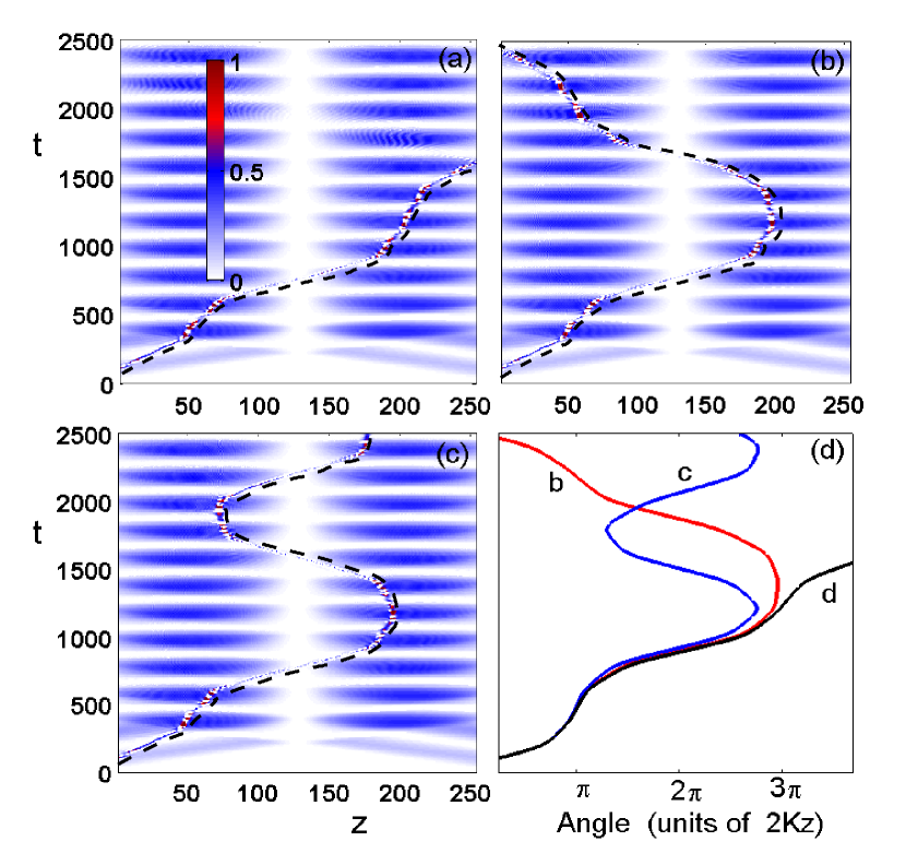
Figure 1: (Color online) Graphs (a), (b) and (c) display results of numerical simulation of (1) under boundary conditions (Numerical simulations.) for the three incident wave amplitudes (24) generating optical lattice with slightly different depths. Graph (d) shows the pendulum angle evolution in model (3) corresponding to those three regimes. For sake of presentation, the gap soliton trajectories have been underlined with dashed lines.

Theory.

We consider an electric field that carries two fundamental frequencies: one is close to the band gap edge $\omega_{0}$, the other is close to zero. Then one deals with a two-wave nonresonant interaction process whose weakly nonlinear limit is sought by assuming the formal series expansion oikawa

$$F=\sum\limits_{p=1}^{\infty}\sum\limits_{\ell=-p}^{p}\varepsilon^{p}F_{\ell}^{(p)}(\xi_{1},\xi_{2},\tau)e^{i\ell[\omega_{0}t+\theta(\xi_{2},\tau)]},$$

$$\xi_{1}=\varepsilon\left[z-\phi(\xi_{2},\tau)\right],\quad\xi_{2}=\varepsilon^{2}z,\quad\tau=\varepsilon^{2}t,$$ (4)

where $F$ stands for any of the three fields $E(z,t)$, $P(z,t)$ or $n(z,t)=1+N(z,t)$. Note that now $n(z,t)$ denotes the normalized population of the excited state. As all components are real valued, we have $\bar{F}_{\ell}^{(n)}=F_{-\ell}^{(n)}$ (overbar stands for complex conjugate). The slow space variables $\xi_{1}$ and $\xi_{2}$ are associated respectively with the characteristic wavelengths of the gap soliton and of the standing wave grating. The above representation actually means to replace the differential operators as follows

$$\frac{d}{dz}\,\to\,\varepsilon\frac{\partial}{\partial\xi_{1}}+\varepsilon^{2}\frac{\partial}{\partial\xi_{2}}-\varepsilon^{3}\frac{\partial\phi}{\partial\xi_{2}}\frac{\partial}{\partial\xi_{1}},$$

$$\frac{d}{dt}\,\to\,i\ell\omega_{0}+\varepsilon^{2}\frac{\partial}{\partial\tau}-\varepsilon^{3}\frac{\partial\phi}{\partial\tau}\frac{\partial}{\partial\xi_{1}},$$ (5)

when applied to a given harmonic $\ell$ of the asymptotic series inserted in (1). This provides the following first order structure of the field

$$E= \varepsilon\big{[}E_{1}^{(1)}(\xi_{1},\tau)e^{i[\omega_{0}t+\theta(\xi_{2},\tau)]}+c.c.\big{]}$$

$$+\varepsilon E_{0}^{(1)}(\xi_{2},\tau)+{\cal O}(\varepsilon^{2}),$$

$$P= -\varepsilon\big{[}E_{1}^{(1)}(\xi_{1},\tau)e^{i[\omega_{0}t+\theta(\xi_{2},\tau)]}+c.c.\big{]}$$

$$+\varepsilon\alpha E_{0}^{(1)}(\xi_{2},\tau)+{\cal O}(\varepsilon^{2}),$$

$$n= {\cal O}(\varepsilon^{2}),$$ (6)

which accounts for the linear limit and deserves some comments. The set of unknowns is: the slowly varying envelope $E_{1}^{(1)}(\xi_{1},\tau)$ of the short wavelength wavepacket (e.g. gap soliton), the very slowly varying profile $E_{0}^{(1)}(\xi_{2},\tau)$ of the long wavelength applied grating, the phase $\theta(\xi_{2},\tau)$ which accounts for variations due to wave-coupling and finally $\phi(\xi_{2},\tau)$ which will be related to the position of the wavepacket by means of (4). Then we note that the expression of the polarization in terms of the electric field actually does follow the usual linear laws $P=-E$ for the plasma wave (here given by $E_{1}^{(1)}e^{i\omega_{0}t}$, the mode at $\omega=\omega_{0}$) and $P=\alpha E$ for the electrostatic component (here given by $E_{0}^{(1)}$, the mode at $\omega=0$). The dependence of these two fields in the slow variables, together with phase variations, will then carry the nonlinear electrodynamics.

Next we seek the leading order ($\varepsilon^{2}$) harmonics of $n(z,t)$. According to the last equation of (1), using (6) and collecting harmonics $\ell=1$ and $\ell=2$, we get after time-integration

$$n^{(2)}_{1}=-E_{1}^{(1)}E_{0}^{(1)},\quad n^{(2)}_{2}=-\frac{1}{2}\big{(}E_{1}^{(1)}\big{)}^{2}.$$ (7)

The last term to compute is $n^{(2)}_{0}$ which cannot be calculated at order $\varepsilon^{2}$ since there, the third equation of (1) is trivial. Thus we move one step further (actually to $\varepsilon^{4}$ to catch the $\tau$-derivative), which provides

$$\frac{\partial n^{(2)}_{0}}{\partial\tau} =-E_{1}^{(1)}\frac{\partial\bar{E}_{1}^{(1)}}{\partial\tau}-\bar{E}_{1}^{(1)}\frac{\partial E_{1}^{(1)}}{\partial\tau}+\alpha E_{0}^{(1)}\frac{\partial E_{0}^{(1)}}{\partial\tau}$$

$$+i\omega_{0}\left[(E^{(3)}_{1}+P^{(3)}_{1})\bar{E}^{(1)}_{1}-c.c.\right].$$ (8)

Then writing the second equation of (1) at order $\varepsilon^{2}$ and using (7), we obtain for $\ell=1$

$$\alpha(P^{(3)}_{1}+E^{(3)}_{1})+2i\omega_{0}\frac{\partial E^{(1)}_{1}}{\partial\tau}-2\omega_{0}E^{(1)}_{1}\frac{\partial\theta}{\partial\tau}$$ (9)

$$-\frac{4+\alpha}{2}\big{|}E_{1}^{(1)}\big{|}^{2}E_{1}^{(1)}+\alpha\big{(}E_{0}^{(1)}\big{)}^{2}E_{1}^{(1)}-\alpha n^{(2)}_{0}E_{1}^{(1)}=0,$$

which is replaced in (Theory.). The result can be integrated to furnish the sought expression

$$n^{(2)}_{0}=\frac{2+\alpha}{\alpha}\left|E_{1}^{(1)}\right|^{2}+\frac{\alpha}{2}\big{(}E_{0}^{(1)}\big{)}^{2}.$$ (10)

Next we consider first equation of (1) at order $\varepsilon^{3}$ and collect again the $\ell=1$ harmonics to get

$$\omega_{0}^{2}\big{(}E^{(3)}_{1}+P^{(3)}_{1}\big{)}+\frac{\partial^{2}E^{(1)}_{1}}{\partial\xi_{1}^{2}}=0.$$ (11)

After some simple algebra we can eliminate $E^{(3)}_{1}$ and $P^{(3)}_{1}$ from equations (9) and (11). The resulting equation appears with terms that depend solely on a single variable, $E^{(1)}_{1}(\xi_{1},\tau)$ on the one side, $\theta(\xi_{2},\tau)$ and $E_{0}^{(1)}(\xi_{2},\tau)$ on the other side. These terms thus decouple to eventually give

$$2i\omega_{0}\frac{\partial E^{(1)}_{1}}{\partial\tau}=\frac{\alpha}{\omega_{0}^{2}}\frac{\partial^{2}E^{(1)}_{1}}{\partial\xi_{1}^{2}}+\frac{4+\alpha}{2}\big{|}E_{1}^{(1)}\big{|}^{2}E_{1}^{(1)},$$ (12)

$$\frac{\partial\theta}{\partial\tau}=-\frac{\alpha(\alpha-2)}{4\omega_{0}}\big{(}E_{0}^{(1)}\big{)}^{2}.$$ (13)

It appears therefore that $E^{(1)}_{1}(\xi_{1},\tau)$ obeys a nonlinear Schrödinger equation where the effect of the applied grating $E_{0}^{(1)}$ lies in the definition of the variable $\xi_{1}$ in (4). Thus the drift $\phi(\xi_{2},\tau)$ remains to be evaluated, which is done with the last equation of (1) at order $\varepsilon^{4}$ and $\ell=1$

$$\frac{\partial\phi}{\partial\tau}=-\frac{\alpha}{\omega_{0}^{3}}\frac{\partial\theta}{\partial\xi_{2}}.$$ (14)

Here we have assumed $E^{(2)}_{1}=0$ which is allowed by the structure of (1) where nonlinearity comes into play at order $\varepsilon^{3}$. Indeed one actually obtains a linear homogeneous equation for $E^{(2)}_{1}$ whose unique solution is $E^{(2)}_{1}=0$ as soon as the initial-boundary value problem concerns only $E^{(1)}_{1}$.

To close the system (12)-(14) we derive the equations for the low frequency oscillations obtained from the first equation of (1) at $\ell=0$, namely

$$\omega_{0}^{2}\,\frac{\partial^{2}E^{(1)}_{0}}{\partial\tau^{2}}-\frac{\partial^{2}E^{(1)}_{0}}{\partial{\xi_{2}}^{2}}=0.$$ (15)

The system (12)-(15) is the basic set of equations that describes within the Maxwell-Bloch model, the interaction of a gap soliton with a long wavelength standing wave. Note that all coefficients are completely determined from the unique parameter $\alpha$, the fundamental coupling constant of eq.(1), as by definition $\omega_{0}^{2}=1+\alpha$. It is useful to eliminate the phase $\theta$ between (13) and (14) and obtain

$$\frac{\partial^{2}\phi}{\partial\tau^{2}}=\frac{\alpha^{2}(\alpha-2)}{4(1+\alpha)^{2}}\frac{\partial}{\partial\xi_{2}}\big{(}E_{0}^{(1)}\big{)}^{2},$$ (16)

which constitutes with (15) a closed system, independently of $E^{(1)}_{1}$.

Application.

We apply now the above machinery to the case when the fundamental field component $E^{(1)}_{1}$ is a gap soliton, exact solution to (12), of given velocity $v_{0}$ in the frame $(\xi_{1},\tau)$. The nature of equation (12) allows us to start with such an explicit solution and then to study its dynamics by looking at the frame drift $\phi(\xi_{2},\tau)$ which thus defines the variations of the soliton about its free motion. To that end it is more convenient to rewrite system (15)(16) in the physical (dimensionless) variables, namely

$$\omega_{0}^{2}\,\frac{\partial^{2}E_{0}}{\partial t^{2}}-\frac{\partial^{2}E_{0}}{\partial z^{2}}=0,$$

$$\frac{\partial^{2}\phi}{\partial t^{2}}=\frac{\alpha^{2}(\alpha-2)}{4(1+\alpha)^{2}}\frac{\partial}{\partial z}\big{(}E_{0}\big{)}^{2},$$ (17)

where $E_{0}(z,t)=\varepsilon E_{0}^{(1)}(\xi_{2},\tau)$. Now the soliton is localized in $\xi_{1}$ and its position, say $z_{s}(t)$, is defined by $\xi_{1}={const}$, namely by $z_{s}-\phi(z_{s},t)={const}$. Computing the velocity $dz_{s}/dt$ and the acceleration $d^{2}z_{s}/dt^{2}$ (total derivatives) we remember that $\phi$ is slowly varying in $z$ and $t$ and thus keep only the dominant orders to eventually obtain

$$\frac{d^{\,2}z_{s}}{dt^{2}}\simeq\left(\frac{\partial^{2}\phi}{\partial t^{2}}\right)_{z=z_{s}}.$$ (18)

We may now select a particular solution to the linear wave equation (15) that would result from application to the medium of two contrapropagating monochromatic beams. The effective boundary conditions that represent such a situation will be described later, they result in the generation of a standing wave at frequency $\Omega$, namely (assuming a system length corresponding to a mode at that frequency)

$$E_{0}={\cal E}\sin(\Omega t)\sin(Kz),\quad K^{2}=(1+\alpha)\Omega^{2}.$$ (19)

Note that the above dispersion law is indeed the behavior at small $\omega$ of the general dispersion law (2). The resulting equation for the soliton acceleration (18) then reads

$$\frac{d^{\,2}z_{s}}{dt^{2}}=K{\cal E}\frac{\alpha^{2}(\alpha-2)}{4(1+\alpha)^{2}}\,\sin^{2}(\Omega t)\,\sin(2Kz_{s}).$$ (20)

This is the parametric driven pendulum equation that can be written as (3) by rescaling time ($\Omega t\to t$) and position ($2Kz_{s}=q$), and by adding a phenomenological damping to account for soliton radiation. Such an equation is solved with the data of initial soliton position $z_{0}$ and velocity $v_{0}$. Our purpose now is to compare the solution of Maxwell-Bloch (1) with convenient boundary data to the prediction of soliton trajectory given by (3).

Numerical simulations.

To proceed with numerical simulations of the MB equations (1) we derive the boundary-value data following chen , that represent incident waves entering the system at $z=0$ and $z=L$ and which are expected to produce the standing low frequency wave (19). The vacuum outside $[0,L]$ is assumed to obey (1) with $\alpha=0$ whose solution reads

$$z\leq 0\,:\quad E_{vac}=I\cos[\Omega(t-z)]+R\cos[\Omega(t+z)].$$ (21)

The amplitude $I$ of the incident wave from the left is the control parameter, the amplitude $R$ of the reflected wave has thus to be eliminated. The continuity conditions at $z=0$ with the electric field $E(z,t)$ inside the medium can be written

$$(I+R)\cos(\Omega t)=\big{(}E\big{)}_{z=0},$$

$$\Omega(I-R)\sin(\Omega t)=\big{(}\partial_{z}E\big{)}_{z=0},$$

which can be combined to eliminate the unknown reflected amplitude $R$ to give

$$\big{(}\partial_{z}E-\partial_{t}E\big{)}_{z=0}=2\Omega I\sin(\Omega t),$$

$$\big{(}\partial_{z}E+\partial_{t}E\big{)}_{z=L}=-2\Omega Q\sin(\Omega t).$$

The above second relation is obtained at t $z=L$ and $Q$ is the chosen amplitude of the incident wave from the right. Such unusual boundary data are actually numerically implemented in a finite difference scheme as (define $L^{-}=L-dz$)

$$E(0,t)=E(dz,t)-dz\,[\partial_{t}E(dz,t)+2\Omega I\sin(\Omega t)],$$

$$E(L,t)=E(L^{-},t)-dz\,[\partial_{t}E(L^{-},t)+2\Omega Q\sin(\Omega t)],$$

which are inserted in the differential equation (1). We shall use equal amplitude out of phase driving, namely $I=-Q$. This generates the standing wave solution (19) whose amplitude ${\cal E}$ is then defined from $I$ by

$${\cal E}=2I\left[(1+\alpha)\cos^{2}(KL/2)+\sin^{2}(KL/2)\right]^{-1/2}.$$ (22)

Then the gap soliton is generated by driving the boundary $z=0$ with an incident pulse at frequency $\omega$ sls and finally the full set of boundary conditions that produce the plots (a), (b) and (c) in fig.1 read

$$\big{(}\partial_{z}E-\partial_{t}E\big{)}_{z=0} =2I\Omega\sin(\Omega t)+\frac{1.393\cos(\omega t)}{\cosh[(t-100)/12]},$$

$$\big{(}\partial_{z}E+\partial_{t}E\big{)}_{z=L} =2I\Omega\sin(\Omega t),$$ (23)

for a system length $L=254$ and initial state at rest: $E(z,0)=0$, $P(z,0)=0$, $N(z,0)=-1$. We choose $\alpha=1$, $\Omega=\pi/200$ and $\omega=1.5$. As defined by (19) the generated standing wave has wavenumber $K=\Omega\sqrt{1+\alpha}$ and its amplitude is defined by (22). The only parameter we vary is the amplitude $I$ of the contrapropagating low frequency beams. In particular the graphs (a), (b) and (c) of fig.1 correspond to the following values

$$2I_{a}=1.832,\qquad 2I_{b}=1.843,\qquad 2I_{c}=1.848.$$ (24)

Why such a small change of the control parameter causes completely different trajectories of the soliton is understood using the pendulum description (3) where in view of (22) the amplitude $A$ is related to the parameters of MB (with $\alpha=1$) by

$$A=I^{2}\left[2\cos^{2}(KL/2)+\sin^{2}(KL/2)\right]^{-1}.$$ (25)

We now solve (3) with initial conditions $z_{s}(0)=0.8$ and $v_{0}=0.94$ that have been measured as the common gap soliton initial position and velocity in the three successive simulations (a), (b) and (c). The phenomenological damping constant is $\gamma=0.01$. Then the pendulum angle evolution for three different values of $A$ resulting from (25) and (24) are displayed in the graph (d) of fig.1.

Conclusion and comments.

It is remarkable that such different models as the Maxwell-Bloch system (1) and the driven parametric pendulum (3) concur to describe the dynamics of a gap soliton interacting with a low-frequency standing wave. This demonstrates in particular that the gap soliton trajectory may well be chaotic, at least initially (it may stabilize due to energy losses by radiationor the internal damping of MB model). This is a direct result of the time dependence of the grating induced by the stationary field. In particular the gap soliton dynamics in a permanent grating (as e.g. a Bragg medium) is regular.

It is worth noting that the effect of damping in initial MB model (1), originating from finite dephasing times, causes eventual transition from chaotic to self trapped regime, as expected from a driven damped pendulum, and which we have checked on numerical simulations. This occurs for time scales of the order of the dephasing times, for which the soliton gets trapped into one of the nodes of the standing wave grating.

One practical advantage of the parametric pendulum description is the prediction of the switching from regular to chaotic (erratic) motion of the gap soliton in terms of the parameters of the driving field. However we expect that the various scenario of chaotic versus periodic motion could be more complex than the driven pendulum case and a more comprehensive analysis would first require much longer computation times, which is a subject of further studies. Beyond such a technical result, our analysis has revealed a new type of soliton motion in a medium with dynamically generated optical grating.

We expect to extend this analysis of a one dimensional time-dependent situation to the study of spatial soliton trajectories in two dimensional smooth optical lattices.

References

- (1) A.C. Scott, Nonlinear Science, 2-nd edition. (Oxford University Press, New York, 2003).
- (2) E. Fermi, J. Pasta, S. Ulam, M. Tsingou, in The Many-Body Problems, edited by D.C. Mattis (World Scientific, Singapore, 1993 reprinted); G. Gallavotti (Ed.) The Fermi-Pasta-Ulam Problem: A status report, Springer (2008).
- (3) I. Siddiqi, R. Vijay, F. Pierre, C.M. Wilson, L. Frunzio, M. Metcalfe, C. Rigetti, R.J. Schoelkopf, M.H. Devoret, D. Vion, D. Esteve, Phys Rev Lett 94 (2005) 027005
- (4) V.M. Fain and Ya.I. Khanin (1969) Quantum Electronics, Pergamon (Oxford, UK)
- (5) R. Khomeriki, J. Leon, Phys Rev Lett 99 (2007) 183601.
- (6) M. Clerc, P. Coullet, E. Tirapegui, Opt. Communications 167 (1999) 159
- (7) J. Starrett, R. Tagg, Phys Rev Lett 74 (1995) 1974
- (8) A.D. Churukian, D.R. Snider, Phys Rev E 53 (1996) 74
- (9) M. Oikawa, N. Yajima, J. Phys. Soc. Japan 37 (1974) 486
- (10) J. Leon, Phys Rev A 75 (2007) 063811
- (11) W. Chen, D.L. Mills, Phys Rev B, 35 (1987), 524