Probability distributions of Linear Statistics in Chaotic Cavities and associated phase transitions.

Abstract

We establish large deviation formulas for linear statistics on the $N$ transmission eigenvalues $\{T_{i}\}$ of a chaotic cavity, in the framework of Random Matrix Theory. Given any linear statistics of interest $A=\sum_{i=1}^{N}a(T_{i})$, the probability distribution $\mathcal{P}_{A}(A,N)$ of $A$ generically satisfies the large deviation formula $\lim_{N\to\infty}\left[-2\log\mathcal{P}_{A}(Nx,N)/\beta N^{2}\right]=\Psi_{A}(x)$, where $\Psi_{A}(x)$ is a rate function that we compute explicitly in many cases (conductance, shot noise, moments) and $\beta$ corresponds to different symmetry classes. Using these large deviation expressions, it is possible to recover easily known results and to produce new formulas, such as a closed form expression for $v(n)=\lim_{N\to\infty}\mathrm{var}(\mathcal{T}_{n})$ (where $\mathcal{T}_{n}=\sum_{i}T_{i}^{n}$) for arbitrary integer $n$. The universal limit $v^{\star}=\lim_{n\to\infty}v(n)=1/2\pi\beta$ is also computed exactly. The distributions display a central Gaussian region flanked on both sides by non-Gaussian tails. At the junction of the two regimes, weakly non-analytical points appear, a direct consequence of phase transitions in an associated Coulomb gas problem. Numerical checks are also provided, which are in full agreement with our asymptotic results in both real and Laplace space even for moderately small $N$. Part of the results have been announced in [P. Vivo, S.N. Majumdar and O. Bohigas, Phys. Rev. Lett. 101, 216809 (2008)].

I Introduction

We consider the statistics of quantum transport through a chaotic cavity with $N_{1}=N_{2}=N\gg 1$ open channels in the two attached leads. It is well established that the electrical current flowing through a cavity of sub-micron dimensions presents time-dependent fluctuations which persist down to zero temperature [1] and are thus associated with the granularity of the electron charge $e$. Among the characteristic features observed in experiments, we can mention weak localization [2], universality in conductance fluctuations [3] and constant Fano factor [4]. In the Landauer-Büttiker scattering approach [1, 5, 6], the wave function coefficients of the incoming and outgoing electrons are related through the unitary scattering matrix $S$ ($2N\times 2N$):

$$S=\begin{pmatrix}r&t^{\prime}\\ t&r^{\prime}\end{pmatrix}$$ (1)

where the transmission ($t,t^{\prime}$) and reflection $(r,r^{\prime})$ blocks are $(N\times N)$ matrices encoding the transmission and reflection coefficients among different channels. Many quantities of interest for the experiments can be extracted from the eigenvalues of the hermitian matrix $tt^{\dagger}$: for example, the dimensionless conductance and the shot noise are given respectively by $G=\mathrm{Tr}(tt^{\dagger})$ [5] and $P=\mathrm{Tr}[tt^{\dagger}(1-tt^{\dagger})]$ [8, 7].

Random Matrix Theory (RMT) has been very successful in describing the statistics of universal fluctuations in such systems, and complements the fruitful semiclassical approach [9, 10, 11, 12, 13]. The simplest way to model the scattering matrix $S$ for the case of chaotic dynamics is to assume that it is drawn from a suitable ensemble of random matrices, with the overall constraint of unitarity [14, 15, 16, 17]. Through a maximum entropy approach with the assumption of ballistic point contacts [1], one derives that the probability distribution of $S$ should be uniform within the unitary group, i.e. $S$ belongs to one of Dyson’s Circular Ensembles [18, 19].

It is then a non trivial task to extract from this information the joint probability density of the transmission eigenvalues $\{T_{i}\}$ of the matrix $tt^{\dagger}$, from which the statistics of interesting experimental quantities could be in principle derived. Fortunately, this can be done [16, 1, 20, 21] and the expression reads:

$$P(T_{1},\ldots,T_{N})=A_{N}\prod_{j<k}|T_{j}-T_{k}|^{\beta}\prod_{i=1}^{N}T_{i}^{\beta/2-1}$$ (2)

where the Dyson index $\beta$ characterizes different symmetry classes ($\beta=1,2$ according to the presence or absence of time-reversal symmetry and $\beta=4$ in case of spin-flip symmetry). The eigenvalues $T_{i}$ are correlated random variables between $0$ and $1$. The constant $A_{N}$ is explicitly known from the celebrated Selberg’s integral as:

$$A_{N}^{-1}=\prod_{j=0}^{N-1}\frac{\Gamma\left(1+\frac{\beta}{2}+j\frac{\beta}{2}\right)\Gamma\left(\frac{\beta}{2}(j+1)\right)\Gamma\left(1+j\frac{\beta}{2}\right)}{\Gamma\left(1+\frac{\beta}{2}\right)\Gamma\left(\frac{\beta}{2}+1+(N+j-1)\frac{\beta}{2}\right)}$$ (3)

From (2), in principle the statistics of all observables of interest can be calculated. In this paper, we shall focus on the following:

$$G =\sum_{i=1}^{N}T_{i}$$ (conductance) (4)

$$P =\sum_{i=1}^{N}T_{i}(1-T_{i})$$ (shot noise) (5)

$$\mathcal{T}_{n} =\sum_{i=1}^{N}T_{i}^{n}$$ (integer moments) (6)

although in principle any linear statistics $A=\sum_{i=1}^{N}a(T_{i})$ can be tackled with the method described below. It is worth mentioning that an increasing interest for the moments and cumulants of the transmission eigenvalues can be observed in recent theoretical [22] and experimental works [23].

Many results are known for the average and the variance of the above quantities, both for large $N$ [1, 24, 25] and, very recently, also for a fixed and finite number of channels $N_{1},N_{2}$ [25, 28, 26, 27]. In particular, a general formula for the variance of any linear statistics $A=\sum_{i=1}^{N}a(\lambda_{i})$ (where $T_{i}=(1+\lambda_{i})^{-1}$) in the limit of large number of open channels is known from Beenakker [29]. However, at least for the case $A=\mathcal{T}_{n}$ (integer moments), this formula is of little practical use. The method we introduce below allows to obtain the sought quantity $v(n)=\lim_{N\to\infty}\mathrm{var}(\mathcal{T}_{n})$ in a neat and explicit way.

In contrast with the case of mean and variance, for which a wealth of results are available (see e.g. [1, 30] and references therein), much less is known for the full distribution of the quantities above: for the conductance, an explicit expression was obtained for $N_{1}=N_{2}=1,2$ [31, 32, 33], while more results are available in the case of quasi one-dimensional wires [34] and 3D insulators [35]. For the shot noise, the distribution was known only for $N_{1}=N_{2}=1$ [36]. Very recently, Sommers et al. [37] announced two formulas for the distribution of the conductance and the shot noise, valid at arbitrary number of open channels and for any $\beta$, which are based on Fourier expansions. Such results are then incorporated and expanded in [38]. In [39] and [40], along with recursion formulas for the efficient computation of conductance and shot noise cumulants, an asymptotic analysis for the distribution functions of these quantities in the limit of many open channels was reported. In a recent letter [41], we announced the computation of the same asymptotics (in the form of large deviation expressions) using a Coulomb gas method and we pointed out a significant discrepancy with respect to the claims by Osipov and Kanzieper [39, 40]. We will discuss in detail such disagreement and the way to sort it out convincingly in subsection IV.4 for the conductance case for $\beta=2$.

Given some recent experimental progresses [42], which made eventually possible to explore the full distribution for the conductance (and not just its mean and variance), it is of great interest to deepen our knowledge about distributions of other quantities, whose experimental test may be soon within reach.

It is the purpose of the present paper to build on [41] and establish exact large deviation formulas for the distribution of any linear statistics on the transmission eigenvalues of a symmetric cavity with $N_{1}=N_{2}=N\gg 1$ open channels. More precisely, for any linear statistics $A$ whose probability density function (pdf) is denoted as $\mathcal{P}_{A}(A,N)$, we have:

$$\lim_{N\to\infty}\left[-\frac{2\log\mathcal{P}_{A}(A=Nx,N)}{\beta N^{2}}\right]=\Psi_{A}(x)$$ (7)

where the large deviation function $\Psi_{A}(x)$ (usually called rate function) is computed exactly for conductance $(A=G)$, shot noise $(A=P)$ and integer moments $(A=\mathcal{T}_{n})$. The method can be extended to the case of asymmetric cavities $N_{1}=\kappa N_{2}$, and is based on a combination of the standard Coulomb gas analogy by Dyson and functional methods recently exploited in [43] in the context of Gaussian random matrices. This approach has been then fruitfully applied to many other problems in statistical physics [51, 44, 45, 46, 47, 48, 49, 50].

The paper is organized as follows. Section II provides a quick summary of our main results. In Section III, we summarize the Coulomb gas method that can in principle be used to obtain the rate function associated with arbitrary linear statistics. In Section IV, V and VI, we use this general method to obtain explicit results respectively for the conductance, shot noise and integer moments. Finally we conclude in Section VII with a summary and some open problems.

II Summary of results

Distribution of conductance $G$: We obtain the following exact expression for the rate function in the case of conductance ($G$)

$$\Psi_{G}(x) =\begin{cases}\frac{1}{2}-\log(4x)&\text{for}\quad 0\leq x\leq\frac{1}{4}\\ 8\left(x-\frac{1}{2}\right)^{2}&\text{for}\quad\frac{1}{4}\leq x\leq\frac{3}{4}\\ \frac{1}{2}-\log[4(1-x)]&\text{for}\quad\frac{3}{4}\leq x\leq 1\end{cases}$$ (8)

The rate function has a quadratic form near its minimum at $x=1/2$ in the range $1/4\leq x\leq 3/4$. Using (7), it then follows that the distribution $\mathcal{P}_{G}(G,N)$ has a Gaussian form close to its peak

$$\mathcal{P}_{G}(G,N)\approx\exp\left(-\frac{\beta}{2}N^{2}\Psi_{G}\left(\frac{G}{N}\right)\right)=\exp\left[-\frac{\beta}{2}N^{2}\cdot 8\left(\frac{G}{N}-\frac{1}{2}\right)^{2}\right]=\exp\left[-\frac{1}{2(1/8\beta)}\left(G-\frac{N}{2}\right)^{2}\right]$$ (9)

from which one easily reads off the mean and variance $\langle G\rangle=N/2$ and $\mathrm{var}(G)=1/8\beta$, which agree with their known large $N$ values. The fact that the variance becomes indepedent of $N$ for large $N$ is referred to as the universal conductance fluctuations. This central Gaussian regime is valid over the region $N/4\leq G\leq 3N/4$. Outside this central zone, $\mathcal{P}_{G}(G,N)$ has non-Gaussian large deviation power law tails. Using (8) in (7) near $x=0$ and $x=1$ , we get $\mathcal{P}_{G}(G,N)\sim G^{\beta N^{2}/2}$ (as $G\to 0$) and $\mathcal{P}_{G}(G,N)\sim(N-G)^{\beta N^{2}/2}$ (as $G\to N$) which are in agreement, to leading order in large $N$, with the exact far tails obtained in  [52, 37, 38]. It turns out that while the central Gaussian regime matches continuously with the two side regimes, there is a weak singularity at the two critical points $G=N/4$ and $G=3N/4$ (only the 3rd derivative is discontinuous). One of our central results is to show that these two weak singularities in the conductance distribution arise due to two phase transitions in the associated Coulomb gas problem where the average charge density undergoes abrupt changes at these critical points. We note that an intermediate regime with an exponential tail claimed in [39, 40] does not appear in our solutions, and we will comment in detail about such discrepancy in subsection IV.4.

Distribution of shot noise $P$: For the shot noise, the exact rate function reads

$$\Psi_{P}(x) =\begin{cases}\frac{1}{4}-2\log 2-\frac{1}{2}\log x&\!\!\!\!\text{for}\quad\!\!\!\!0\leq x\leq\frac{1}{16}\\ 64\left(x-\frac{1}{8}\right)^{2}&\!\!\!\!\text{for}\quad\!\!\!\!\frac{1}{16}\leq x\leq\frac{3}{16}\\ \frac{1}{4}-2\log 2-\frac{1}{2}\log\left(\frac{1}{4}-x\right)&\!\!\!\!\text{for}\quad\!\!\!\!\frac{3}{16}\leq x\leq\frac{1}{4}\end{cases}$$ (10)

Thus the shot noise distribution $\mathcal{P}_{P}(P,N)$, in the large $N$ limit, also has a central Gaussian regime over $N/16\leq P\leq 3N/16$ where

$$\mathcal{P}_{P}(P,N)\approx\exp\left(-\frac{\beta}{2}N^{2}\Psi_{P}\left(\frac{P}{N}\right)\right)=\exp\left[-\frac{\beta}{2}N^{2}\cdot 64\left(\frac{P}{N}-\frac{1}{8}\right)^{2}\right]=\exp\left[-\frac{1}{2(1/64\beta)}\left(P-\frac{N}{8}\right)^{2}\right]$$ (11)

yielding $\langle P\rangle=N/8$ and $\mathrm{var}(P)=1/64\beta$. As in the case of conductance, this central Gaussian regime is flanked on both sides by two non-Gaussian power law tails with weak third order singularities at the transition points $P=N/16$ and $P=3N/16$.

Distribution of integer moments $\mathcal{T}_{n}$: For general $n>1$, the computation of the full rate function $\Psi_{\mathcal{T}_{n}}(x)$ and hence the large $N$ behavior of the distribution $\mathcal{P}_{\mathcal{T}_{n}}(\mathcal{T}_{n},N)$ turns out to be rather cumbersome. However, the distribution $\mathcal{P}_{\mathcal{T}_{n}}(\mathcal{T}_{n},N)$ shares some common qualitative features with the conductance and the shot noise distributions. For example, we show that for any $n>1$, there is a central Gaussian regime where the rate function $\Psi_{\mathcal{T}_{n}}(x)$ has a quadratic form given exactly by:

$$\Psi_{\mathcal{T}_{n}}(x)=\frac{b_{n}}{2}\left[x-\frac{\Gamma(n+1/2)}{\sqrt{\pi}\Gamma(n+1)}\right]^{2}$$ (12)

where $b_{n}=\frac{4\pi\Gamma(n)\Gamma(n+1)}{[\Gamma(n+1/2)]^{2}}$. This implies a Gaussian peak in the distribution:

$$\mathcal{P}_{\mathcal{T}_{n}}(\mathcal{T}_{n},N)\approx\exp\left[-\frac{\beta}{2}N^{2}\frac{b_{n}}{2}\left[\frac{\mathcal{T}_{n}}{N}-\frac{\Gamma(n+1/2)}{\sqrt{\pi}\Gamma(n+1)}\right]^{2}\right]$$ (13)

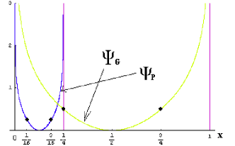
Figure 1: (Color online). $\Psi_{G}(x)$ and $\Psi_{P}(x)$ as in (8) and (10). The black dots highlight the critical points on each curve.

from which one easily reads off the mean and variance of integer moments:

$$\langle\mathcal{T}_{n}\rangle =\frac{N\Gamma(n+1/2)}{\sqrt{\pi}\Gamma(n+1)}$$ (14)

$$\mathrm{var}(\mathcal{T}_{n}) =\frac{2}{\beta b_{n}}=\frac{[\Gamma(n+1/2)]^{2}}{2\beta\pi\Gamma(n)\Gamma(n+1)}$$ (15)

To the best of our knowledge, the latter result, together with its universal asymptotic value $\lim_{n\to\infty}\mathrm{var}(\mathcal{T}_{n})=(2\beta\pi)^{-1}$, has not been reported previously in the literature.

As in the case of conductance and shot noise, there are singular points separating the central Gaussian regime and the non-Gaussian tails. However, the situation is more complicated for $n>1$. Unlike in the conductance or the shot noise case where there are only two phase transitions separating three regimes, there are more regimes for $n>1$. We analyse here in detail the case $n=2$ where we show that there are actually three singular points separating $4$ regimes. This is again a consequence of phase transitions in the associated Coulomb gas problems where the average charge density undergoes abrupt changes at these critical points. It would be interesting to see how many such phase transitions occur for $n>2$. However, we do not have any simple way to predict this and this remains an interesting open problem. The tails of the distribution for the integer moments case can be computed in principle for general $n>1$, and the formalism is developed in section VI, but for clarity we will focus mostly on the case $n=2$. The left tail has again a power-law decay for any $n>1$.

III Summary of the Coulomb gas method

It is useful to summarize briefly the method we use to compute the distribution of linear statistics in the large $N$ limit. Given a linear statistics of interest $A=\sum_{i=1}^{N}a(T_{i})$, its probability density function (pdf) $\mathcal{P}_{A}(A,N)$, using the joint pdf of $T_{i}$’s in Eq. (2), is given by

$$\mathcal{P}_{A}(A,N)=A_{N}\int_{0}^{1}\cdots\int_{0}^{1}dT_{1}\cdots dT_{N}\exp\left(\frac{\beta}{2}\sum_{j\neq k}\log|T_{j}-T_{k}|+\left(\frac{\beta}{2}-1\right)\sum_{i=1}^{N}\log T_{i}\right)\delta\left(\sum_{i=1}^{N}a(T_{i})-A\right).$$ (16)

The main idea then is to work with its Laplace transform

$$\mathbf{F}_{N}\left(z;A\right)=\int_{0}^{\infty}dA\ \mathcal{P}_{A}(A,N)e^{-\frac{\beta}{2}zA}$$ (17)

where the variable $z$ takes in principle complex values and its dependence on $N$ is at present unspecified.

Suppose one is able to compute the following limit:

$$J_{A}(p)=-\frac{2}{\beta}\lim_{N\to\infty}\frac{\log\mathbf{F}_{N}\left(N^{\alpha}p;A\right)}{N^{2}}$$ (18)

and such limit is finite and nonzero for a certain speed $\alpha$ and for $p\in\mathbb{R}$ such that $p\sim\mathcal{O}(1)$ for $N\to\infty$. It is then a classical result in large deviation theory (Gärtner-Ellis theorem, see e.g. [53] Appendix C) that the following finite nonzero limit exists:

$$\Psi_{A}(x)=-\frac{2}{\beta}\lim_{N\to\infty}\frac{\log\mathcal{P}_{A}\left(N^{\alpha}x,N\right)}{N^{2}}$$ (19)

and $\Psi_{A}(x)$ [the rate function] is given by the inverse Legendre transform of $J_{A}(p)$:

$$\Psi_{A}(x)={\rm max}_{p}\left[J_{A}(p)-p\,x\right].$$ (20)

Note that:

1. There is no need to consider complex values for $z$ (and thus for $p$) in (17), as only real values matter for obtaining the rate function. As $\mathcal{P}_{A}(A,N)$ has generically a compact support, negative values for $p$ are also allowed.

2. Setting the appropriate speed $\alpha$ is evidently crucial for obtaining a finite nonzero limit in (18). There is no freedom in here. Conversely, any speed is equally good when extracting the cumulants out of the Laplace transform (17) $(z=N^{\alpha}p)$ through the formula (set $\beta=2$ for simplicity):

   $$\kappa_{\ell}(A)=\left(\frac{-1}{N^{\alpha}}\right)^{\ell}\frac{\partial^{\ell}}{\partial p^{\ell}}\log\mathbf{F}_{N}(N^{\alpha}p;A)\Big{|}_{p=0}$$ (21)

   as no limiting procedure is performed in (21).

3. The rate function $\Psi_{A}(x)$ encodes the full information about the probability distribution in the limit of infinitely many open channels. However, our numerical simulations confirm that it also gives a fairly accurate description of such distribution for rather small $N$.

What is then the correct speed $\alpha$ for the linear statistics considered here? It is quite easy to argue that $\alpha$ must be set equal to $1$. The reason is best understood by taking the conductance $G=\sum_{i=1}^{N}T_{i}$ for $\beta=2$ as an example. By very general arguments we expect the large $N$ behavior of $\mathcal{P}_{G}(G,N)$ to scale as $\mathcal{P}_{G}(G,N)\sim e^{-N^{2}\Psi_{G}(G/N)}$ for large $N$. Clearly, the two exponentials (the one coming from $\mathcal{P}_{G}(G,N)$ and the other coming from the Laplace measure) must be of the same order in $N$ to guarantee a meaningful saddle point contribution, and since $G\sim N$ for large $N$, clearly $z\sim N$ as well.

After setting the proper speed, we get in full generality:

$$\underbrace{\int_{0}^{\infty}\mathcal{P}_{A}(A,N)e^{-\frac{\beta}{2}NpA}dA}_{\mathbf{F}_{N}(Np;A)}=A_{N}\int_{0}^{1}\!\!\!\!\cdots\!\!\!\int_{0}^{1}dT_{1}\cdots dT_{N}\exp\left(\frac{\beta}{2}\sum_{j\neq k}\log|T_{j}-T_{k}|+\left(\frac{\beta}{2}-1\right)\sum_{i=1}^{N}\log T_{i}-\frac{\beta}{2}pN\sum_{i=1}^{N}a(T_{i})\right).$$ (22)

We can write the exponential as, $\exp\left[-\beta E(\{T_{i}\})\right]$ with $E(\{T_{i}\})=-(1/2)\sum_{j\neq k}\log|T_{j}-T_{k}|+\sum_{i}V(T_{i})$ where $V(T)=(1/\beta-1/2)\,\log(T)+pNa(T)/2$. This representation provides a natural Coulomb gas interpretation. We can identify $T_{i}$’s as the coordinates of the charges of a $2$-d Coulomb gas that lives on a one dimensional real segment $[0,1]$. The charges repel each other via the $2$-d logarithmic Coulomb potential and in addition, they sit in an external potential $V(T)$. Note that the Laplace parameter $p$ appears explicitly in the external potential $V(T)$. Then $E$ is the energy of this Coulomb gas. Thus one can write the Laplace transform as the ratio of two partition functions

$$\mathbf{F}_{N}\left(Np;A\right)=\int_{0}^{\infty}\mathcal{P}_{A}(A,N)e^{-\frac{\beta}{2}NpA}dA=\frac{Z_{p}(N)}{Z_{0}(N)}$$ (23)

where $Z_{p}(N)$ is precisely the multiple integral on the rhs of Eq. (22) and $Z_{0}(N)=1/A_{N}$ (which simply follows by putting $p=0$ in Eq. (22) and using the fact that the pdf $\mathcal{P}_{A}(A,N)$ is normalized to unity).

The next step is to evaluate this partition function $Z_{p}(N)$ of the Coulomb gas in the large $N$ limit. This procedure for the large $N$ calculation was originally introduced by Dyson [19] and has recently been used in the context of the largest eigenvalue distribution of Gaussian [43] and Wishart random matrices [51] and also in other related problems of counting stationary points in random Gaussian landscapes [44]. There are two basic steps involved. The first step is a coarse-graining procedure where one sums over (partial tracing) all microscopic configurations of $T_{i}$’s compatible with a fixed charge density function $\varrho_{p}(T)=N^{-1}\sum_{i}\delta(T-T_{i})$ and the second step consists in performing a functional integral over all possible positive charge densities $\varrho_{p}(T)$ that are normalized to unity. Finally the functional integral is carried out in the large $N$ limit by the saddle point method.

Following this general procedure summarized in  [43], the resulting functional integral, to leading order in large $N$, becomes:

$$Z_{p}(N)\propto\int\mathcal{D}[\varrho_{p}]e^{-\frac{\beta}{2}N^{2}S[\varrho_{p}]}$$ (24)

where the action is given by

$$S[\varrho_{p}] =p\int_{0}^{1}\varrho_{p}(T)\,a(T)dT+B\left[\int_{0}^{1}\varrho_{p}(T)dT-1\right]$$

$$-\int_{0}^{1}\int_{0}^{1}dTdT^{\prime}\varrho_{p}(T)\varrho_{p}(T^{\prime})\log|T-T^{\prime}|.$$ (25)

Here $B$ is a Lagrange multiplier enforcing the normalization of $\varrho_{p}(T)$. In the large $N$ limit, the functional integral in (24) is particularly suitable to be evaluated by the saddle point method, i.e., one finds the solution $\varrho_{p}^{\star}(T)$ (the equilibrium charge density that minimizes the action or the free energy) from the stationarity condition $\delta S[\varrho_{p}]/\delta\varrho_{p}=0$ which leads to an integral equation

$$V_{\rm ext}(T)=p\,a(T)+B=2\int_{0}^{1}\varrho_{p}^{\star}(T^{\prime})\,\log|T-T^{\prime}|\,dT^{\prime}$$ (26)

where $V_{\rm ext}(T)=pa(T)+B$ is termed as external potential. Differentiating once with respect to $T$ leads to a singular integral equation

$$\frac{p}{2}\,a^{\prime}(T)={\rm Pr}\int_{0}^{1}\frac{\varrho_{p}^{\star}(T^{\prime})}{T-T^{\prime}}dT^{\prime}$$ (27)

where ${\rm Pr}$ denotes the principal part and $a^{\prime}(T)=da/dT$.

Assuming one can solve (27) for $\varrho_{p}^{\star}$, one next evaluates the action $S[\varrho_{p}]$ in (III) at the stationary solution $\varrho_{p}^{\star}$ and then takes the ratio in (23) to get (upon comparison with (18)):

$$\underbrace{\int_{0}^{\infty}\mathcal{P}_{A}(A,N)e^{-\frac{\beta}{2}NpA}dA}_{\mathbf{F}_{N}(Np;A)}\approx e^{-\frac{\beta}{2}N^{2}[\overbrace{S[\varrho_{p}^{\star}]-S[\varrho_{0}^{\star}]}^{J_{A}(p)}]}.$$ (28)

Inverting the Laplace transform gives the main asymptotic result $\mathcal{P}(A,N)\approx\exp\left(-\frac{\beta}{2}N^{2}\Psi_{A}\left(\frac{A}{N}\right)\right)$ where the rate function is the inverse Legendre transform (see (20)),

$$\Psi_{A}(x)=\max_{p}[-x\,p+J_{A}(p)]$$ (29)

with $J_{A}(p)$ given by the free energy difference as in (28).

To summarize, given any linear statistics $a(T)$, the steps are: (i) solve the singular integral equation (27) for the density $\varrho_{p}^{\star}(T)$ (ii) evaluate the action $S[\varrho_{p}^{\star}]$ in (III) (iii) evaluate $J_{A}(p)=S[\varrho_{p}^{\star}]-S[\varrho_{0}^{\star}]$ and finally (iv) use $J_{A}(p)$ in (29), maximize the rhs to evaluate the rate function $\Psi_{A}(x)$. We will see later that all these steps can be carried out fully and explicitly when $A=G$ (conductance) and $A=P$ (shot noise) and partially when $A=\mathcal{T}_{n}$ (integer moments).

The important first step is to find the explicit solution of the singular integral equation (27). Note that this equation is of the Poisson form and it is, in some sense, an inverse electrostatic problem: given the potential $p\,a^{\prime}(T)$, we need to find the charge density $\varrho_{p}^{\star}(T)$. To proceed, we recall a theorem due to Tricomi [54] concerning the general solution to singular integral equations of the form

$$g(x)=\mathrm{Pr}\int_{a}^{b}\frac{f(x^{\prime})}{x-x^{\prime}}dx^{\prime}$$ (30)

where $g(x)$ is given and one needs to find $f(x)$ which has only a single support over the interval $[a,b]$ with $a<b$ (the lower edge $a$ should not be confused with the linear statistics function $a(T)$). The solution $f(x)$, with a single support over $[a,b]$ can be found explicitly [54]

$$f(x)=-\frac{1}{\pi^{2}\sqrt{(b-x)(x-a)}}\left[\mathrm{Pr}\int_{a}^{b}\frac{\sqrt{(b-x^{\prime})(x^{\prime}-a)}}{x-x^{\prime}}g(x^{\prime})dx^{\prime}+B_{1}\right]$$ (31)

where $B_{1}$ is an arbitrary constant.

In our case, $g(x)=p\,a^{\prime}(x)/2$ and provided we assume that the charge density has a single support over $[a,b]$ with $a<b$, we can in principle use this solution (31). However, if the solution happens to have a disconnected support one cannot use this formula directly. Whether the solution has a single or disconnected support depends, of course, on the function $a(T)$. We will see that indeed for the case of conductance ($a(T)=T$), the solution has a single support and one can use (31) directly. The edges $a$ and $b$ in that case are determined self-consistently as explained in Section IV. On the other hand, for the shot noise ($a(T)=T(1-T)$) and for integer moments with $n>1$ ($a(T)=T^{n}$), it turns out that for certain values of the parameter $p$, the solution has a disconnected support. In that case, one cannot use (31) directly. However, we will see later that one can still obtain the solution explicitly by an indirect application of (31).

A very interesting feature of (27) is that, depending on the value of the Laplace parameter $p$, the fluid of charged particles undergoes a series of real phase transitions in Laplace space, i.e., as one varies the Laplace parameter $p$, there are certain critical values of $p$ at which the solution $\varrho_{p}^{\star}(T)$ abruptly changes its form. As a consequence, the rate function, related to the Laplace transform via the Legendre transform (29), also undergoes a change of behavior as one varies its argument at the corresponding critical points. The rate function is continuous at these critical points but it has weak non-analiticities (characterized by a discontinuous third derivative).

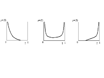
Figure 2: Phases of the density of transmission eigenvalues for the conductance case.

As an example, we consider the case of the conductance ($a(T)=T$) (see section IV for details). In fig. 2, we plot schematically the saddle point density $\varrho_{p}^{\star}(T)$ (solution of (27) with $a(T)=T$), for three different intervals on the real $p$ line. We will see in the next section that there are three possible solutions valid respectively for $p\geq 4$, $-4\leq p\leq 4$ and $p\leq-4$.

• when $p\geq 4$, the external potential $V_{\rm ext}(T)=p\,T+B$ is strong enough (compared to the logarithmic repulsion) to keep the fluid particles confined between the hard wall at $T=0$ and a point $L_{1}=4/p$. The gas particles accumulate towards $T\to 0^{+}$, where the density develops an inverse square root divergence, while $\varrho_{p}^{\star}(L_{1})=0$. This situation is depicted in the left panel of fig. 2;

• when $p$ hits the critical value $p^{(+)}=4$ from above, the density profile changes abruptly. The external potential $V_{\mathrm{ext}}$ is no longer overcoming the logarithmic repulsion, so the fluid particles spread over the whole support $(0,1)$, and the density generically exhibits an inverse square root divergence at both endpoints ($T\to 0^{+}$ and $T\to 1^{-}$). This phase keeps holding for all the values of $p$ down to the second critical point $p^{(-)}=-4$ (see the second panel in fig. 2), when the negative slope of the potential is so steep that the particles can no longer spread over the whole support $(0,1)$, but prefer to be located near the right hard edge at $T=1$.

• In the third phase $(p<-4)$, the fluid particles are pushed away from the origin and accumulate towards the right hard wall at $T\to 1$ (see the rightmost panel in fig. 2). The density thus vanishes below the point $L_{2}=1-4/|p|$.

It is worth mentioning that such phase transitions in the solutions of integral equations have been observed recently in other systems that also allow similar Coulomb gas representations. These include bipartite quantum entanglement problem [55], nonintersecting fluctuating interfaces in presence of a substrate [47] and also multiple input multiple output (MIMO) channels [56].

IV Distribution of the conductance

We start with the simplest case of linear statistics, namely the conductance $G=\sum_{i=1}^{N}T_{i}$. Thus in this case $a(T)=T$ is simply a linear function. Substituting $a(T)=T$ in (26) gives

$$V_{\rm ext}(T)=p\,T+B=2\int_{0}^{1}\varrho_{p}^{\star}(T^{\prime})\log|T-T^{\prime}|dT^{\prime}$$ (32)

and then (27) becomes

$$\frac{p}{2}=\mathrm{Pr}\int_{0}^{1}\frac{\varrho_{p}^{\star}(T^{\prime})}{T-T^{\prime}}dT^{\prime}$$ (33)

We have then to find the solution to (33). Once this solution $\varrho_{p}^{\star}(T)$ is found, we can evaluate the action $S[\varrho_{p}^{\star}]$ at the saddle point in the following way. Multiplying (32) by $\varrho_{p}^{\star}(T)$ and integrating (using the normalization $\int_{0}^{1}\varrho_{p}^{\star}(T)dT=1$) gives

$$p\int_{0}^{1}T\varrho_{p}^{\star}(T)\,dT+B =2\int_{0}^{1}\int_{0}^{1}\varrho_{p}^{\star}(T)\,\varrho_{p}^{\star}(T^{\prime})\times$$

$$\times\log|T-T^{\prime}|\,dT\,dT^{\prime}.$$ (34)

Next we use this result to replace the double integral term in the action in (III) (with $a(T)=T$) to get

$$S[\varrho_{p}^{\star}]=\frac{p}{2}\int_{0}^{1}\varrho_{p}^{*}(T)TdT-\frac{B}{2}.$$ (35)

The yet unknown constant $B$ is determined from (32) upon using the explicit solution, once found.

To find the solution to (33) explicitly we will use the general Tricomi formula in (31) assuming a single support over $[a,b]$. The edges $a$ and $b$ will be determined self-consistently. Physically, we can foresee three possible forms for the density $\varrho_{p}^{\star}(T)$ according to the strength and sign of the external potential $V_{\rm ext}(T)=p\,T+B$ on the left hand side (lhs) of (32).

1. For large and positive $p$, the fluid particles (transmission eigenvalues) will feel a strong confining potential which keeps them close to the left hard edge $T\to 0+$. Thus, $\varrho_{p}^{\star}(T)$ will have a support $[0,L_{1}]$, with $0<L_{1}<1$.

2. For intermediate values of $p$, the particles will spread over the full range $[0,1]$.

3. For large and negative $p$, the fluid particles will be pushed towards the right edge and the support of $\varrho_{p}^{\star}(T)$ will be over $[L_{2},1]$, with $0<L_{2}<1$.

These three cases will correspond to different solutions for the Tricomi equation (33) above, and the positivity constraint for the obtained densities will fix the range of variability for $p$ in each case. Once a solution $\varrho_{p}^{\star}(T)$ for each case (different ranges for $p$) is obtained, we can then use (35) to evaluate the action at the saddle point.

Let us consider the three cases discussed above separately.

IV.1 Large $p$: support on $[0,L_{1}]$

We assume that the solution is nonzero over the support $[0,L_{1}]$ based on our physical intuition for large $p$, where $L_{1}$ is yet unknown. We use the general Tricomi solution with a single support in (31) with $a=0$, $b=L_{1}$ and $g(x)=p/2$ giving

$$\varrho_{p}^{\star}(T)=-\frac{1}{\pi^{2}\sqrt{T(L_{1}-T)}} \left[\frac{p}{2}~{}\mathrm{Pr}\int_{0}^{L_{1}}\frac{\sqrt{T^{\prime}(L_{1}-T^{\prime})}}{T-T^{\prime}}dT^{\prime}\right.$$

$$\left.+B_{1}\right]$$ (36)

where $B_{1}$ is an arbitrary constant. Evaluating the principal value integral on the rhs of (IV.1) we get

$$\varrho_{p}^{\star}(T)=\frac{p}{2\pi\sqrt{T}}\sqrt{L_{1}-T}$$ (37)

where the constant $B_{1}$ has been determined using the fact that the density $\varrho_{p}^{\star}(T)$ must vanish at the upper edge $T=L_{1}$. The normalization of $\varrho_{p}^{\star}(T)$ gives:

$$L_{1}=\frac{4}{p},\qquad L_{1}<1\Rightarrow p>4$$ (38)

As expected, this solution holds for large values of $p$ (i.e. for a strong confining potential).

Since the point $T=0$ belongs to the support $[0,L_{1}]$, we can put $T=0$ in (32) to determine the constant $B$

$$B=2\int_{0}^{1}\varrho_{p}^{\star}(T^{\prime})\log T^{\prime}dT^{\prime}$$ (39)

Substituting $B$ in (35) gives the saddle point action

$$S[\varrho_{p}^{\star}]=\frac{p}{2}\int_{0}^{1}\varrho_{p}^{\star}(T)TdT-\int_{0}^{1}\varrho_{p}^{\star}(T)\log(T)dT$$ (40)

Performing the integrals using the explicit solution $\varrho_{p}^{\star}(T)$ (37) gives a very simple expression, valid for $p>4$,

$$S[\varrho_{p}^{\star}]=3/2+\log p$$ (41)

In Fig. 3 we show the results from a Montecarlo simulation to test the prediction (37) for the average density of eigenvalues in Laplace space for $p>4$. The numerical density for $N$ eigenvalues (here and for all the subsequent cases) is obtained as:

$$\varrho_{p}^{\star}(x_{1})\simeq\frac{\Big{\langle}e^{-pN\sum_{i=1}^{N}x_{i}}\prod_{j<k}|x_{j}-x_{k}|^{2}\Big{\rangle}_{N-1}}{\Big{\langle}e^{-pN\sum_{i=1}^{N}x_{i}}\prod_{j<k}|x_{j}-x_{k}|^{2}\Big{\rangle}_{N}}$$ (42)

where the average $\Big{\langle}\cdot\Big{\rangle}$ is taken over $N-1$ random numbers ${x_{2},\ldots,x_{N}}$ (numerator) with a flat measure over $[0,1]$, with $x_{1}$ spanning the interval $(0,1)$. In the denominator, the normalization constant is obtained with the same procedure, this time averaging over $N$ random variables uniformly drawn from $(0,1)$. In all cases, the agreement with the theoretical results is fairly good already for $N=5$.

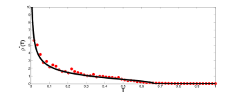
Figure 3: (Color online). Density of transmission eigenvalues $T$ for $N=5$ and $p=6$ (theory vs. numerics) for the conductance case.

IV.2 Intermediate $p$: support on the full range $[0,1]$

In this case, the solution of (33) from (31) reads:

$$\varrho_{p}^{\star}(T)=\frac{p}{2\pi\sqrt{T(1-T)}}\left[K-T\right]$$ (43)

The normalization of $\varrho_{p}^{\star}(T)$ determines $K=(4+p)/{2p}$. Now, depending on whether $p>0$ or $p<0$, there are 2 positivity constraints ($\varrho_{p}^{\star}(T)>0$ everywhere) to take into account:

1. if $p>0$, the positivity constraint $K-1>0$ at the upper edge $T=1$ implies $p<4$.

2. if $p<0$, the positivity constraint $K<0$ at the lower edge $T=0$ implies $p>-4$.

Thus the solution (43) with support over the full alllowed range $[0,1]$ is valid for all $-4\leq p\leq 4$.

Substituting this solution into the simplified action (40) (which holds in this case as well) gives:

$$S[\varrho_{p}^{\star}]=-\frac{p^{2}}{32}+\frac{p}{2}+2\log 2$$ (44)

Note that since this range $-4\leq p\leq 4$ includes, in particular the $p=0$ case, we can use the expression in (44) to evaluate the value of the action at $p=0$ that will be required later in evaluating the large deviation function via (28). Putting $p=0$ in (44) gives

$$S[\varrho_{0}^{\star}]=2\log 2.$$ (45)

In fig. 4, we plot the analytical result for the density together with Montecarlo simulations for $N=5$ and $p=1$.

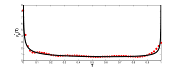
Figure 4: (Color online). Density of transmission eigenvalues $T$ for $N=5$ and $p=1$ (theory vs. numerics) for the conductance case.

IV.3 Large negative $p$: support on $[L_{2},1]$

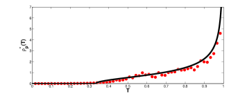
Figure 5: (Color online). Density of transmission eigenvalues $T$ for $N=5$ and $p=-6$ (theory vs. numerics) for the conductance case.

In this case, the solution of (33) reads:

$$\varrho_{p}^{\star}(T)=\frac{|p|}{2\pi\sqrt{1-T}}\sqrt{T-L_{2}},\qquad L_{2}=1-\frac{4}{|p|}$$ (46)

The implications for the $p$-range are as follows:

$$L_{2}>0\Rightarrow p<-4$$ (47)

Note that we can no longer use the expression for the constant $B$ in (39) since now the allowed range of the solution $[L_{2},1]$ does not include the point $T=0$. Instead, putting $T=1$ in (32), we determine the value of $B$ as

$$B=2\int_{0}^{1}\varrho_{p}^{\star}(x^{\prime})\log|1-x^{\prime}|dx^{\prime}-p$$ (48)

Substituting $B$ in (35) we get a new expression for the action at the saddle point

$$S[\varrho_{p}^{\star}]=\frac{p}{2}\int_{0}^{1}dTT\,\varrho_{p}^{\star}(T)-\int_{0}^{1}dT\varrho_{p}^{\star}(T)\,\log|1-T|+\frac{p}{2}$$ (49)

Evaluating (49) using the solution in (46) gives the saddle point action for $p<-4$

$$S[\varrho_{p}^{\star}]=3/2+p+\log(-p)$$ (50)

In fig. 5, we plot the analytical result for the density together with Montecarlo simulations for $N=5$ and $p=-6$.

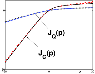
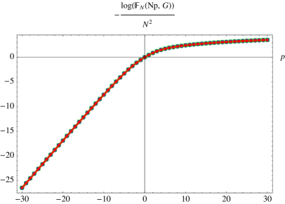
Figure 6: (Color online). Left: $J_{G}(p)$ and $J_{Q}(p)$ vs. Montecarlo simulations (see eq. (70) and (80)). Right: our asymptotic predictions $J_{G}(p)$ (solid red line) is compared with the exact finite $N$ expression (59) from [39] for $N=4$ (green squares) and $N=10$ (blue dots). Already for $N=4$, our large $N$ formula again matches the exact finite $N$ result with accuracy up to the second decimal digit over the full real $p$ range.

IV.4 Comparison with other theories and numerical simulations

As summarized in the next section, we obtained for the rate function of the conductance for $\beta=2$, defined as (see (19)):

$$\Psi_{G}(x)=-\lim_{N\to\infty}\frac{\log\mathcal{P}_{G}(Nx,N)}{N^{2}}$$ (51)

the following expression (limited to $x\in[1/2,1]$, given the symmetry $\Psi_{G}(x)=\Psi_{G}(1-x)$):

$$\Psi_{G}(x)=\begin{cases}8\left(x-\frac{1}{2}\right)^{2}&1/2\leq x\leq 3/4\\ \frac{1}{2}-\log[4(1-x)]&3/4\leq x<1\end{cases}$$ (52)

In [39], Osipov and Kanzieper (OK) claim a different limiting law, namely:

$$\Psi_{G}^{\rm{OK}}(x)=\begin{cases}8\left(x-\frac{1}{2}\right)^{2}&1/2\leq x\leq 3/4\\ 4x-\frac{5}{2}&3/4\leq x<1\end{cases}$$ (53)

and $\Psi_{G}^{\rm{OK}}(x)$ would approach the form in (52) (second line) only at the extreme edge $x\to 1^{-}$ (over a narrow region of order $1/N$).

Which law is then correct? There is a conclusive way to settle this dispute, namely to compare the two theoretical results to a direct numerical simulation of $\mathcal{P}_{G}(G,N)$. We will present simulation results in Laplace space which agree very well with our result on the Laplace transform (see fig. 6, left panel, and equations (65) and (70) in next section) over the full range of real $p$ values, as well as a convincing comparison with the exact finite $N$ result for the same observable using the Hankel determinant representation (59) from [39] (see fig. 6, right panel). We shall argue below that OK asymptotic theory is instead unable to reproduce the tails of $J_{G}(p)$ for $|p|>4$, which are responsible for long power-law tails in the rate function $\Psi_{G}(x)$. Since, however, working in the Laplace space may not appear conclusive as far as the real-space rate function $\Psi_{G}(x)$ is concerned, it would be better if one could perform a simulation directly for $\mathcal{P}_{G}(G,N)$ and not just for its Laplace transform.

Indeed, it turns out to be quite easy to simulate directly $\mathcal{P}_{G}(G,N)$ using an elementary and standard Monte Carlo Metropolis algorithm which we describe below.

Monte Carlo method:

The main problem is to compute the distribution of the conductance $G$ which, for a fixed number of channels $N$ and $\beta=2$, is given by the multiple integral

$$\mathcal{P}_{G}(G,N)\!=\!\!A_{N}\,\!\!\!\int_{0}^{1}\prod_{i=1}^{N}dT_{i}\prod_{i<j}(T_{i}-T_{j})^{2}\,\delta\left(\sum_{i=1}^{N}T_{i}-G\right)$$ (54)

where the prefactor $A_{N}$ is set by the normalization: $\int_{0}^{\infty}\mathcal{P}_{G}(G,N)dG=1$ and is known exactly for all $N$ (see eq. (3)).

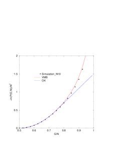
Figure 7: (Color online). Comparison between Montecarlo simulations for the rate function $\Psi(x)=-\lim_{N\to\infty}\log\mathcal{P}_{G}(Nx,N)/N^{2}$ as a function of $x=G/N$ for $\beta=2$ (black dots), our asymptotic theory (VMB) (continuous red line) and the theory by Osipov-Kanzieper (OK) (dashed blue line). Simulations are performed for $N=10$ (left) and $N=50$ (right), which allows to appreciate the convergence to our theoretical curve as $N$ is increased.

To employ the Monte Carlo method, we first write the integrand (the Vandermonde term) in (54)

$$\prod_{i<j}(T_{i}-T_{j})^{2}=e^{-E\{T_{i}\}};\hskip 4.0ptE\{T_{i}\}=-\sum_{i\neq j}\ln\left(|T_{i}-T_{j}|\right).$$ (55)

Thus, one can interpret $0\leq T_{i}\leq 1$ as the position of an $i$-th charge in a one dimensional box $[0,1]$ and the charges interact via the logarithmic Coloumb energy $-E\{T_{i}\}$. This Coulomb gas is in thermal equilibrium with a Gibbs weight $\exp[-E\{T_{i}\}]$ for any configuration $\{T_{i}\}$, where the inverse temperature is set to $1$.

It is then very easy and standard to simulate the equilibrium properties of this gas via a Monte Carlo method [57]. We start from any configuration $\{T_{i}\}$. We pick a particle, say the $i$-th one, at random and attempt to move its position by an amount $\delta$: $T_{i}\to T_{i}+\delta$. This move causes a change in energy $\Delta E$ of the gas. According to the standard Metropolis algorithm [57], the move is accepted with probability $e^{-\Delta E}$ if $\Delta E>0$ and with probability $1$ if $\Delta E<0$. The move is rejected if the new position $T_{i}+\delta$ is outside the box $[0,1]$. This Metropolis move guarantees that after a large number of microscopic moves, the system reaches the stationary distribution with the correct Boltzmann weight $e^{-E\{T_{i}\}}$.

We wait for a long enough time to ensure that the system has indeed reached equilibrium. After that we let the system evolve according to these microscopic moves and construct the normalized histogram $\mathcal{P}_{G}(G,N)$ of $G=\sum_{i=1}^{N}T_{i}$. Once again, we are guaranteed that $T_{i}$’s are sampled with the correct equilibrium weight. This procedure allows us to simulate fairly large systems. To obtain good statistics for the distribution over the full range of $x=G/N$, i.e., over $1/2\leq x\leq 1$, we implement an iterative conditional sampling method, used in other contexts before [49], that allows us to generate events with extremely small probabilities at the far tail of the distribution [58].

In Fig. 7, we plot $\Psi(x)=-\ln[\mathcal{P}_{G}(G,N)]/N^{2}$ vs the scaling variable $x=G/N$ for $1/2\leq x\leq 1$ for $N=50$. The black dots show the simulation points. The red (solid) line shows our (VMB) result in (52), while the blue (dashed) line shows the OK prediction (53). Clearly the two results agree with each other, as well as with the simulations, in the Gaussian regime $1/2\leq x\leq 3/4$. However, in the outer region $3/4\leq x<1$, while the VMB result in (52) is in perfect agreement with the simulation results, the OK result in (53) deviates widely from them. This proves conclusively that in the regime $3/4\leq x<1$, the VMB result (52) is correct and the OK result (53) is incorrect.

There is another way to see that the OK asymptotics can not be correct. Since OK theory stems from the asymptotic analysis of the following integral representation for the probability distribution of conductance (see eq. 22 of [39]):

$$\mathcal{P}_{G}^{\rm{(OK)}}(G,N)=\frac{2N^{1/4}}{\Gamma(1/8)}\sqrt{\frac{2}{\pi}}\int_{0}^{\infty}d\lambda\frac{e^{-N^{2}\left(\lambda+\frac{2\eta^{2}}{1+2\lambda}\right)}}{\lambda^{7/8}\sqrt{1+2\lambda}}$$ (56)

where $\eta=2(G/N)-1$, we can now compute from (56) the same observable we considered here, namely:

$$J_{G}(p)=-\lim_{N\to\infty}\frac{\log\mathbf{F}_{N}(Np;G)}{N^{2}}$$ (57)

for $p\in\mathbb{R}$ and $p\sim\mathcal{O}(1)$ for $N\to\infty$ (see equations (17) and (18)), and thus compare once again the large $N$ predictions of VMB and OK theories against i) numerical simulations, and ii) the exact finite $N$ result, which is fortunately available (see fig. 6).

Inserting (56) into the definition of the Laplace transform (17), we obtain after simple algebraic steps:

$$\mathbf{F}_{N}(Np;G) =\frac{N^{1/4}}{\Gamma(1/8)}\exp\left(-N^{2}\left(\frac{p}{2}-\frac{p^{2}}{32}\right)\right)\times$$

$$\times\underbrace{\int_{0}^{\infty}d\lambda\frac{e^{-N^{2}\lambda\left(1-p^{2}/16\right)}}{\lambda^{7/8}}}_{\phi_{N}(p)}$$ (58)

The integral $\phi_{N}(p)$ clearly does not converge for $|p|\geq 4$, with the consequence that OK integral representation (56) fails to reproduce the tails of both:

• Montecarlo simulations of $J_{G}(p)$ (see fig. 6, left panel),

• the exact finite $N$ result [39] for the Laplace transform in terms of a Hankel determinant (see fig. 6, right panel):

  $$\mathbf{F}_{N}(Np;G)=\frac{N!}{c_{N}}\det\left[(-\partial_{z})^{j+k}\frac{1-e^{-z}}{z}\Big{|}_{z=Np}\right]_{0\leq j,k\leq N-1},\qquad c_{N}=\prod_{j=0}^{N-1}\frac{\Gamma(j+2)\Gamma^{2}(j+1)}{\Gamma(j+N+1)}$$ (59)

which evidently do exist and are perfectly captured instead by our approach in both cases.

Within the range of validity $|p|<4$, the integral $\phi_{N}(p)$ can be evaluated and gives eventually:

$$\mathbf{F}_{N}(Np;G)=\frac{\exp\left(-N^{2}(p/2-p^{2}/32)\right)}{(1-p^{2}/16)^{1/8}},\qquad\qquad\mbox{if }|p|<4$$ (60)

Note that all $N$-dependence has completely dropped out from the prefactor, leaving us with two perfectly compatible (even though apparently discordant at first glance) consequences:

1. According to OK theory, the limit

   $$J_{G}(p)=-\lim_{N\to\infty}\frac{\log\mathbf{F}_{N}(Np;G)}{N^{2}}=p/2-p^{2}/32\qquad\mbox{for }|p|<4$$ (61)

   which is correct but incomplete (as their integral has nothing to say about the tails $|p|\geq 4$).

2. Not surprisingly then, from the OK theory, the leading $(1/N)$ order of the cumulants of the distribution, computed through the formula (21):

   $$\kappa_{\ell}(G)=\left(\frac{-1}{N}\right)^{\ell}\frac{\partial^{\ell}}{\partial p^{\ell}}\log\mathbf{F}_{N}(Np;G)\Big{|}_{p=0}$$ (62)

   is correctly reproduced (see also [38] for an independent calculation of such cumulants, which is in perfect agreement with OK result).

In summary, the OK integral representation in (56) is only adequate around the Gaussian peak (the $p=0$ neighborhood in Laplace space, which is exactly the only region which cumulants probe (see (62))), and in this neighborhood it has the merit of producing the correct leading $1/N$ term of the expansion of such cumulants (unattainable by our method) and confirmed independently in [38]. Outside this region, however, the OK integral representation is invalid and the asymptotic analysis of it outside its range of validity obviously produces an incorrect result. Note also that, for any fixed $N$ (however large), one has from (56) that $\mathcal{P}_{G}^{\rm{(OK)}}(G=0,N)=\mathcal{P}_{G}^{\rm{(OK)}}(G=N,N)>0$ strictly, while it is well-known that the density must vanish identically at the edges [37, 38, 52] for any $N$. This simple observation rules out the claims of exactness of (56) in [39].

IV.5 Final results for the conductance case

To summarize, the density of eigenvalues (solution of the saddle point equation (33)) has the following form:

$$\varrho_{p}^{\star}(T)=\begin{cases}\frac{p}{2\pi\sqrt{T(1-T)}}\left[\frac{4+p}{2p}-T\right]&\qquad 0\leq T\leq 1\qquad-4\leq p\leq 4\\ \frac{p}{2\pi\sqrt{T}}\sqrt{\frac{4}{p}-T}&\qquad 0\leq T\leq 4/p\qquad p\geq 4\\ \frac{|p|}{2\pi\sqrt{1-T}}\sqrt{T-(1-4/|p|)}&\qquad 1-4/|p|\leq T\leq 1\qquad p\leq-4\end{cases}$$ (63)

One may easily check that $\varrho_{p}^{\star}(T)$ is continuous at $p=\pm 4$, but develops two phase transitions characterized by different supports.

The action at the saddle point is given by:

$$S[\varrho_{p}^{\star}]=\begin{cases}-\frac{p^{2}}{32}+\frac{p}{2}+2\log 2&-4\leq p\leq 4\\ 3/2+\log p&p\geq 4\\ 3/2+p+\log(-p)&p\leq-4\end{cases}$$ (64)

which is again continuous at $p=\pm 4$.

Using the above expressions for the saddle point action and the result in (45), the expression for the free energy difference $J_{G}(p)=S[\varrho_{p}^{\star}]-S[\varrho_{0}^{\star}]$ follows from (28):

$$J_{G}(p)=\begin{cases}-\frac{p^{2}}{32}+\frac{p}{2}&-4\leq p\leq 4\\ 3/2+\log(p/4)&p\geq 4\\ 3/2+p+\log(-p/4)&p\leq-4\end{cases}$$ (65)

Using this expression for $J_{G}(p)$ in the Legendre transform (29) and maximizing gives the exact expression for the rate function

$$\Psi_{G}(x)=\begin{cases}8\left(x-\frac{1}{2}\right)^{2}&\frac{1}{4}\leq x\leq\frac{3}{4}\\ \frac{1}{2}-\log(4x)&0\leq x\leq\frac{1}{4}\\ \frac{1}{2}-\log[4(1-x)]&\frac{3}{4}\leq x\leq 1\end{cases}$$ (66)

From this formula, one can derive the leading behavior of the tails of $\mathcal{P}_{G}(G,N)$ as:

$$\mathcal{P}_{G}(G,N) \stackrel{{\scriptstyle G\to 0}}{{\approx}}\exp\left\{-\frac{\beta}{2}N^{2}\left[-\log\left(4G/N\right)\right]\right\}=G^{\beta N^{2}/2}$$ (67)

$$\mathcal{P}_{G}(G,N) \stackrel{{\scriptstyle G\to N}}{{\approx}}\exp\left\{-\frac{\beta}{2}N^{2}\left[-\log\left(4(1-G/N)\right)\right]\right\}=$$

$$=(N-G)^{\beta N^{2}/2}$$

in agreement with [37, 38, 52].

The most interesting feature of (66) is the appearance of discontinuities in higher-order derivatives at the critical points: more precisely, the third derivative of $\Psi_{G}(x)$ is discontinuous at $x=1/4$ and $x=3/4$. In fact, Sommers et al [37] found that for finite $N_{1},N_{2}$ there are several non-analytical points. Only two of them survive to the leading order $N\to\infty$ and, in our picture, these correspond to a physical phase transition in Laplace space.

In summary, the following exact limit holds:

$$\lim_{N\to\infty}\left[-\frac{2\log\mathcal{P}_{G}(Nx,N)}{\beta N^{2}}\right]=\Psi_{G}(x)$$ (69)

where the rate function $\Psi_{G}(x)$ is given in (66).

The free energy difference in Laplace space (65) for large $N$ has been compared with:

1. Montecarlo simulations over the range $p=(-30,30)$, which already for $N=5$ show an excellent agreement (see fig. 6, left panel). For a given $p$ between $-30$ and $30$, the numerical $J_{G}(p)$ (and analogously for $J_{Q}(p)$) is computed as:

   $$J_{G}(p)\simeq\frac{\Big{\langle}e^{-pN\sum_{i=1}^{N}x_{i}}\prod_{j<k}|x_{j}-x_{k}|^{2}\Big{\rangle}_{N}}{\Big{\langle}\prod_{j<k}|x_{j}-x_{k}|^{2}\Big{\rangle}_{N}}$$ (70)

   where the average is taken over $N$ random variables $\{x_{i}\}$ drawn from a uniform distribution over $(0,1)$.

2. the exact finite $N$ result from [39] for the Laplace transform of the density in terms of a Hankel determinant (see (59)). In fig. 6 (right panel), we plot our asymptotic result $J_{G}(p)$ (65) together with $-\log\mathbf{F}_{N}(Np;G)/N^{2}$, where $\mathbf{F}_{N}(Np;G)$ is the exact finite $N$ result (59) for the Laplace transform from [39], for $-30\leq p\leq 30$ and $N=4,10$. Already for $N=4$, our $J_{G}(p)$ reproduces the exact finite $N$ formula with an accuracy of two decimal digits.

V Distribution of the shot noise

The dimensionless shot noise is defined as $P=\sum_{i=1}^{N}T_{i}(1-T_{i})$ [8, 7]. It is convenient to rewrite it in the form $P=N/4-\sum_{i=1}^{N}(1/2-T_{i})^{2}=N/4-Q$. The probability distributions of $P$ and $Q$ are related by:

$$\mathcal{P}_{P}(P,N)=\mathcal{P}_{Q}\left(\frac{N}{4}-P,N\right)$$ (71)

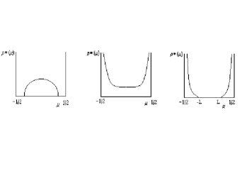
Figure 8: Density of the auxiliary $Q$ (schematic).

It is also necessary to make the change of variable in the joint pdf (2) $\mu_{i}=1/2-T_{i}$, so that $-1/2\leq\mu_{i}\leq 1/2$. The joint pdf (2) expressed in terms of the new variables $\mu_{i}$ reads:

$$P(\mu_{1},\ldots,\mu_{N})=A_{N}\prod_{j<k}|\mu_{j}-\mu_{k}|^{\beta}\prod_{i=1}^{N}\left(\frac{1}{2}-\mu_{i}\right)^{\frac{\beta}{2}-1}$$ (72)

and we are interested in the large $N$ decay of the logarithm of $\mathcal{P}_{Q}(Q,N)$, where $Q=\sum_{i}\mu_{i}^{2}$. We have:

$$\mathcal{P}_{Q}(Q,N)=A_{N}\int_{-1/2}^{1/2}\cdots\int_{-1/2}^{1/2}d\mu_{1}\cdots d\mu_{N}\exp\left(\frac{\beta}{2}\sum_{j\neq k}\log|\mu_{j}-\mu_{k}|+\left(\frac{\beta}{2}-1\right)\sum_{i=1}^{N}\log\left(\frac{1}{2}-\mu_{i}\right)\right)\delta\left(\sum_{i=1}^{N}\mu_{i}^{2}-Q\right)$$ (73)

Again, taking the Laplace transform and converting multiple integrals to functional integrals we obtain:

$$\int_{0}^{\infty}\mathcal{P}_{Q}(Q,N)e^{-\frac{\beta}{2}NpQ}dQ=A_{N}\int\mathcal{D}[\varrho]e^{-\frac{\beta}{2}N^{2}S[\varrho_{p}]}$$ (74)

where for notational simplicity we keep the same symbols $\varrho_{p}$ and $S$ as before. Of course, the new action $S$ reads:

$$S[\varrho_{p}]=p\int_{-1/2}^{1/2}\varrho_{p}(\mu)\mu^{2}d\mu-\int_{-1/2}^{1/2}\int_{-1/2}^{1/2}d\mu d\mu^{\prime}\varrho_{p}(\mu)\varrho_{p}(\mu^{\prime})\log|\mu-\mu^{\prime}|+C\left[\int_{-1/2}^{1/2}\varrho_{p}(\mu)d\mu-1\right]$$ (75)

where $C$ is the new Lagrange multiplier enforcing the normalization of the charge density to unity.

The stationary point of the action $S$ is determined by:

$$\frac{\delta S[\varrho_{p}]}{\delta\varrho_{p}}=0$$ (76)

yielding:

$$p{\mu}^{2}+C=2\int_{-1/2}^{1/2}d{\mu}^{\prime}\varrho_{p}^{\star}({\mu}^{\prime})\log|\mu-{\mu}^{\prime}|$$ (77)

Taking one more derivative with respect to $\mu$, we get to the following Tricomi equation:

$$p\mu=\mathrm{Pr}\int_{-1/2}^{1/2}\frac{\varrho_{p}^{\star}({\mu}^{\prime})}{\mu-{\mu}^{\prime}}d{\mu}^{\prime}$$ (78)

In terms of the solution $\varrho_{p}^{\star}(\mu)$ of (78), the action (75) can be simplified as:

$$S[\varrho_{p}^{\star}]=\frac{p}{2}\int_{-1/2}^{1/2}\varrho_{p}^{\star}(\mu){\mu}^{2}d\mu-\frac{C}{2}$$ (79)

where the value of the constant $C$ is determined from (77) by attributing a value to $\mu$ within the support of the solution. As in the conductance case, we can write the asymptotic decay of $Q$ as:

$$\int_{0}^{\infty}\mathcal{P}_{Q}(Q,N)e^{-\frac{\beta}{2}NpQ}dQ\approx\exp\left(-\frac{\beta}{2}N^{2}\{S[\varrho_{p}^{\star}]-S[\varrho_{0}^{\star}]\}\right)=\exp\left(-\frac{\beta}{2}N^{2}J_{Q}(p)\right)$$ (80)

Again, in order to solve (78) we need first to foresee the structure of the allowed support for $\varrho_{p}^{\star}(\mu)$. This time, the symmetry constraint $\varrho_{p}^{\star}(\mu)=\varrho_{p}^{\star}(-\mu)$ reduces the possible behaviors of $\varrho_{p}^{\star}(\mu)$ to the following three cases: I) $\varrho_{p}^{\star}(\mu)$ has compact support $[-L,L]$ with $L<1/2$, or II) $\varrho_{p}^{\star}(\mu)$ has non-compact support $(-1/2,1/2)$, or III) the support of $\varrho_{p}^{\star}(\mu)$ is the union of two disjoint semi-compact intervals $(-1/2,-L]\cup[L,1/2)$ with $L>0$ (see Fig. 8). We analyze the three cases separately.

V.1 Support on $[-L,L]$ with $L<1/2$

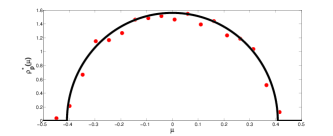
Figure 9: (Color online). Density of shifted transmission eigenvalues $\mu$ for $N=6$ and $p=12$ (theory vs. numerics) for the shot noise case.

The general solution of (78) in this case is given by:

$$\varrho_{p}^{\star}(\mu)=\frac{p}{\pi\sqrt{L^{2}-{\mu}^{2}}}[c_{1}-{\mu}^{2}]$$ (81)

The constant $c_{1}$ is clearly determined as $c_{1}=L^{2}$ by the condition that $\varrho_{p}^{\star}(\pm L)=0$. Thus, the solution within the bounds $[-L,L]$ with $L<1/2$ is the semicircle:

$$\varrho_{p}^{\star}(\mu)=\frac{p}{\pi}\sqrt{L^{2}-{\mu}^{2}}$$ (82)

where the edge point $L$ is determined by the normalization condition $\int_{-L}^{L}\varrho_{p}^{\star}(\mu)d\mu=1$. This gives:

$$L=\sqrt{\frac{2}{p}},\qquad L<1/2\Rightarrow p>8$$ (83)

So, eventually (see Fig. 9):

$$\varrho_{p}^{\star}(\mu)=\frac{p}{\pi}\sqrt{\frac{2}{p}-{\mu}^{2}},\qquad-\sqrt{\frac{2}{p}}\leq\mu\leq\sqrt{\frac{2}{p}},\qquad p>8$$ (84)

Evaluating the action (79) (after determining the constant $C$ from (77) by putting $\mu=0$ there) we get for $p>8$:

$$S[\varrho_{p}^{\star}]=\frac{3}{4}+\frac{1}{2}\log 2+\frac{1}{2}\log p$$ (85)

From (80), the value of $J_{Q}(p)=S[\varrho_{p}^{\star}]-S[\varrho_{0}^{\star}]$ (still using $S[\varrho_{0}^{\star}]=2\log 2$) for $p\geq 8$ is given by:

$$J_{Q}(p)=\frac{3}{4}+\frac{1}{2}\log\left(\frac{p}{8}\right)$$ (86)

Again, the rate function $\Psi_{Q}(x)$ is given by the inverse Legendre transform of (86), i.e.:

$$\Psi_{Q}(x)=\max_{p}\left[-xp+J_{Q}(p)\right]=\frac{1}{4}-2\log 2-\frac{1}{2}\log x$$ (87)

valid for $0\leq x\leq 1/16$. From (71), we have the following relation among the rate functions for $Q$ and $P$:

$$\Psi_{P}(x)=\Psi_{Q}\left(\frac{1}{4}-x\right)$$ (88)

implying for $\Psi_{P}(x)$ the following expression:

$$\Psi_{P}(x)=\frac{1}{4}-2\log 2-\frac{1}{2}\log\left(\frac{1}{4}-x\right)\qquad\text{for}\quad\frac{3}{16}\leq x\leq\frac{1}{4}$$ (89)

In fig. 9 we plot the theoretical density of shifted transmission eigenvalues together with Montecarlo simulations for $N=6$ and $p=12$.

V.2 Support on $(-1/2,1/2)$

The general solution of (78) in this case is given by:

$$\varrho_{p}^{\star}(\mu)=\frac{p}{\pi\sqrt{1/4-{\mu}^{2}}}[b_{1}-{\mu}^{2}]$$ (90)

The constant $b_{1}$ is determined by the normalization condition $\int_{-1/2}^{1/2}\varrho_{p}^{\star}(\mu)d\mu=1$. This gives $b_{1}=1/p+1/8$. In turn, the positivity constraint for the density implies $-8<p<8$. We then get:

$$\varrho_{p}^{\star}(\mu)=\frac{p}{\pi\sqrt{1/4-{\mu}^{2}}}\left[\frac{1}{p}+\frac{1}{8}-{\mu}^{2}\right],\qquad-\frac{1}{2}<\mu<\frac{1}{2},\qquad-8<p<8$$ (91)

Evaluating the action (79) gives for $-8<p<8$:

$$S[\varrho_{p}^{\star}]=\frac{p}{8}-\frac{p^{2}}{256}+2\log 2$$ (92)

From (80), the value of $J_{Q}(p)=S[\varrho_{p}^{\star}]-S[\varrho_{0}^{\star}]$ for $-8\leq p\leq 8$ is given by:

$$J_{Q}(p)=-\frac{p^{2}}{256}+\frac{p}{8}$$ (93)

Again, the rate function $\Psi_{Q}(x)$ is given by the inverse Legendre transform of (93), i.e.:

$$\Psi_{Q}(x)=\max_{p}\left[-xp+J_{Q}(p)\right]=64\left(x-\frac{1}{8}\right)^{2}$$ (94)

valid for $1/16\leq x\leq 3/16$. From the relation (88), we have for $\Psi_{P}(x)$ the following expression:

$$\Psi_{P}(x)=64\left(\frac{1}{8}-x\right)^{2}\qquad\text{for}\quad\frac{1}{16}\leq x\leq\frac{3}{16}$$ (95)

In fig. 10 we plot the theoretical density of shifted transmission eigenvalues together with Montecarlo simulations for $N=6$ and $p=1$.

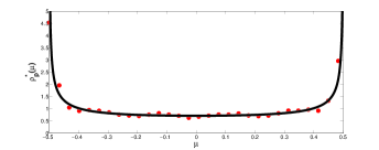
Figure 10: (Color online). Density of shifted transmission eigenvalues $\mu$ for $N=6$ and $p=1$ (theory vs. numerics) for the shot noise case.

V.3 Support on $(-1/2,-L]\cup[L,1/2)$

For large negative values of $p$, we envisage a form for the charge density as in fig. 8 (rightmost panel), i.e. on a disconnected support with two connected and symmetric components. This is because for large negative $p$, the external potential $p{\mu}^{2}$ in (77) tends to push the charges to the two extreme edges of the box $0$ and $1$, creating an empty space in the middle. Since we expect to have a disconnected support, we cannot directly use the single support Tricomi solution (31). We need to proceed differently.

We start by recasting eq. (78) in the following form:

$$p\mu =\int_{-1/2}^{-L}\frac{\varrho_{p}^{\star}({\mu}^{\prime})}{\mu-{\mu}^{\prime}}d{\mu}^{\prime}+\mathrm{Pr}\int_{L}^{1/2}\frac{\varrho_{p}^{\star}({\mu}^{\prime})}{\mu-{\mu}^{\prime}}d{\mu}^{\prime} \quad\mu>0$$ (96)

$$p\mu =\mathrm{Pr}\int_{-1/2}^{-L}\frac{\varrho_{p}^{\star}({\mu}^{\prime})}{\mu-{\mu}^{\prime}}d{\mu}^{\prime}+\int_{L}^{1/2}\frac{\varrho_{p}^{\star}({\mu}^{\prime})}{\mu-{\mu}^{\prime}}d{\mu}^{\prime} \quad\mu<0$$ (97)

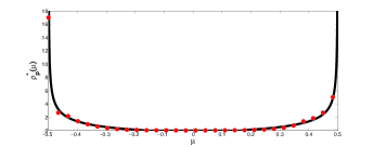
Figure 11: (Color online). Density of shifted transmission eigenvalues $\mu$ for $N=4$ and $p=-9$ (theory vs. numerics) for the shot noise case.

In the rhs of (96) (first integral) we make the change of variables ${\mu}^{\prime}\to-{\mu}^{\prime}$, getting:

$$p\mu =\int_{L}^{1/2}\frac{\varrho_{p}^{\star}(-{\mu}^{\prime})}{\mu+{\mu}^{\prime}}d{\mu}^{\prime}+\mathrm{Pr}\int_{L}^{1/2}\frac{\varrho_{p}^{\star}({\mu}^{\prime})}{\mu-{\mu}^{\prime}}d{\mu}^{\prime}$$ (98)

Exploiting the symmetry $\varrho_{p}^{\star}(\mu)=\varrho_{p}^{\star}(-\mu)$, we get:

$$p\mu =\mathrm{Pr}\int_{L}^{1/2}d{\mu}^{\prime}\varrho_{p}^{\star}({\mu}^{\prime})\left[\frac{1}{\mu+{\mu}^{\prime}}+\frac{1}{\mu-{\mu}^{\prime}}\right]$$

$$=2\mu\ \mathrm{Pr}\int_{L}^{1/2}d{\mu}^{\prime}\frac{\varrho_{p}^{\star}({\mu}^{\prime})}{{\mu}^{2}-{\mu}^{\prime 2}}$$ (99)

Making a further change of variables ${\mu}^{2}=y,{\mu}^{\prime 2}=y^{\prime}$ we get eventually a Tricomi equation for $\tilde{\varrho}_{p}(\mu)=\varrho_{p}^{\star}(\sqrt{\mu})/\sqrt{\mu}$ as:

$$p =\mathrm{Pr}\int_{L^{2}}^{1/4}dy^{\prime}\frac{\tilde{\varrho}_{p}(y^{\prime})}{y-y^{\prime}}$$ (100)

Solving (100) by the standard one support solution (31) and converting back to $\varrho_{p}^{\star}(\mu)$ we get:

$$\varrho_{p}^{\star}(\mu)=\frac{|p\mu|(a_{2}-{\mu}^{2})}{\pi\sqrt{(1/4-{\mu}^{2})({\mu}^{2}-L^{2})}}$$ (101)

where $a_{2}$ is an arbitrary constant, fixed by the condition $\varrho_{p}^{\star}(\pm L)=0$ (the density is vanishing at the edge points). This gives $a_{2}=L^{2}$. Imposing the normalization condition, we get $L^{2}=1/4-2/|p|$. The condition that $L\geq 0$ implies that this solution is valid when $p\leq-8$. Thus for $p\leq-8$, we then get:

$$\varrho_{p}^{\star}(\mu)=\frac{|p\mu|\sqrt{{\mu}^{2}-1/4+2/|p|}}{\pi\sqrt{1/4-{\mu}^{2}}}$$ (102)

Note that, when $p\to-8$ from below, the equilibrium solution (102) smoothly matches the solution (91) in the intermediate regime. The action is readily evaluated from (79) as:

$$S[\varrho_{p}^{\star}] =p\int_{L}^{1/2}d\mu{\mu}^{2}\varrho_{p}^{\star}(\mu)-2\int_{L}^{1/2}d\mu\varrho_{p}^{\star}(\mu)\log\mu$$

$$=\frac{3}{4}+\frac{1}{2}\log(|p|)-\frac{|p|}{4}+\frac{1}{2}\log 2$$ (103)

The corresponding $J_{Q}(p)$ is given by:

$$J_{Q}(p)=\frac{3}{4}+\frac{1}{2}\log\left(\frac{|p|}{8}\right)-\frac{|p|}{4}$$ (104)

from which the rate function $\Psi_{Q}(x)$ can be easily derived:

$$\Psi_{Q}(x)=\max_{p}[-xp+J_{Q}(p)]=\frac{1}{4}-2\log 2-\frac{1}{2}\log\left(\frac{1}{4}-x\right)\qquad 3/16\leq x\leq 1/4$$ (105)

In fig. 11 we plot the theoretical density of shifted transmission eigenvalues together with Montecarlo simulations for $N=4$ and $p=-9$.

V.4 Final results for the shot noise case

To summarize, the density of the shifted eigenvalues $\{\mu_{i}\}$ (solution of the saddle point equation (78)) has the following form:

$$\varrho_{p}^{\star}(\mu)=\begin{cases}\frac{p}{\pi}\sqrt{\frac{2}{p}-{\mu}^{2}}&\qquad-\sqrt{\frac{2}{p}}\leq\mu\leq\sqrt{\frac{2}{p}}\qquad p\geq 8\\ \frac{p}{\pi\sqrt{1/4-{\mu}^{2}}}\left[\frac{8+p}{8p}-{\mu}^{2}\right]&\qquad-1/2\leq\mu\leq 1/2\qquad-8\leq p\leq 8\\ \frac{|p\mu|\sqrt{{\mu}^{2}-1/4+2/|p|}}{\pi\sqrt{1/4-{\mu}^{2}}}&\qquad-1/2\leq\mu\leq-\sqrt{1/4-2/|p|}\vee\sqrt{1/4-2/|p|}\leq\mu\leq 1/2\qquad p\leq-8\end{cases}$$ (106)

One may easily check that $\varrho_{p}^{\star}(\mu)$ is continuous at $p=\pm 8$, but develops two phase transitions characterized by different supports.

The saddle-point action (79) is given by:

$$S[\varrho_{p}^{\star}]=\begin{cases}\frac{3}{4}+\frac{1}{2}\log 2+\frac{1}{2}\log p&p>8\\ \frac{p}{8}-\frac{p^{2}}{256}+2\log 2&-8\leq p\leq 8\\ \frac{3}{4}+\frac{1}{2}\log(|p|)-\frac{|p|}{4}+\frac{1}{2}\log 2&p\leq-8\end{cases}$$ (107)

which is again continuous at $p=\pm 8$.

From (28), the expression of $J_{Q}(p)=S[\varrho_{p}^{\star}]-S_{0}[\varrho_{0}^{\star}]$ is:

$$J_{Q}(p)=\begin{cases}\frac{3}{4}+\frac{1}{2}\log\left(\frac{p}{8}\right)&p\geq 8\\ \frac{-p^{2}}{256}+\frac{p}{8}&-8\leq p\leq 8\\ \frac{3}{4}+\frac{1}{2}\log\left(\frac{|p|}{8}\right)-\frac{|p|}{4}&p\leq-8\end{cases}$$ (108)

from which one can derive (in complete analogy with the conductance case) the rate function for the auxiliary quantity $Q$:

$$\Psi_{Q}(x)=\begin{cases}\frac{1}{4}-2\log 2-\frac{1}{2}\log x&0\leq x\leq 1/16\\ 64\left(x-\frac{1}{8}\right)^{2}&1/16\leq x\leq 3/16\\ \frac{1}{4}-2\log 2-\frac{1}{2}\log\left(\frac{1}{4}-x\right)&3/16\leq x\leq 1/4\end{cases}$$ (109)

and from the relation $\Psi_{P}(x)=\Psi_{Q}(1/4-x)$ one readily obtains the rate function for the shot noise in (10).

VI Distribution of moments $\mathcal{T}_{n}$ for integer $n$

In this section, we deal with the more general case of integer moments $\mathcal{T}_{n}=\sum_{i=1}^{N}T_{i}^{n}$, in particular focussing on the case $n=2$. The conductance is exactly given by $\mathcal{T}_{1}$ while the shot noise is $\mathcal{T}_{1}-\mathcal{T}_{2}$. While we could use the general method outlined in Section III with the choice $a(T)=T^{n}$, as was done for the conductance case ($n=1$), it turns out that one can obtain the same final results by using a short-cut which combines, in one step, the saddle point evaluation in (26) and the maximization of the Legendre transform in (29). Of course, both methods finally yield the same results, but this shortcut explicitly avoids any Laplace inversion. Here, we illustrate the short-cut method for the case $a(T)=T^{n}$, but it can also be used for other linear statistics.

The distribution of the moments $\mathcal{P}_{\mathcal{T}_{n}}(\mathcal{T}_{n}=Nt,N)$ is given by:

$$\mathcal{P}_{\mathcal{T}_{n}}(\mathcal{T}_{n}=Nt,N)=A_{N}\int_{0}^{1}\cdots\int_{0}^{1}dT_{1}\cdots dT_{N}\exp\left(\frac{\beta}{2}\sum_{j\neq k}\log|T_{j}-T_{k}|+\left(\frac{\beta}{2}-1\right)\sum_{i=1}^{N}\log T_{i}\right)\delta\left(\sum_{i=1}^{N}T_{i}^{n}-Nt\right)$$ (110)

The short-cut consists in replacing the delta function by its integral representation: $\delta(x)=\int\frac{dp}{2\pi}e^{px}$ where the integral runs in the complex $p$ plane. The rest is as before, namely that in the large $N$ limit, one replaces the multiple integral by a functional integral introducing a continuous charge density $\varrho_{p}(x)$. This gives

$$\mathcal{P}_{\mathcal{T}_{n}}(\mathcal{T}_{n}=Nt,N)=A_{N}\int\frac{dp}{2\pi}\mathcal{D}[\varrho]e^{-\frac{\beta}{2}N^{2}S[\varrho_{p}]}$$ (111)

where the action is given by:

$$S[\varrho_{p}]=p\left(\int_{0}^{1}\varrho_{p}(x)x^{n}dx-t\right)-\int_{0}^{1}\int_{0}^{1}dxdx^{\prime}\varrho_{p}(x)\varrho_{p}(x^{\prime})\log|x-x^{\prime}|+C\left[\int_{0}^{1}\varrho_{p}(x)dx-1\right]$$ (112)

where the rhs of (111) is now extremized with respect to both $\varrho(x)$ and $p$. Notice that here we have already performed the inverse Laplace transform of (23). Hence the two methods are exactly identical.

Extremizing the action gives the following saddle point equations:

$$px^{n}+C =2\int_{0}^{1}~{}dx^{\prime}\varrho_{p}^{\star}(x^{\prime})\log|x-x^{\prime}|$$ (113)

$$t =\int_{0}^{1}~{}dxx^{n}\varrho_{p}^{\star}(x)$$ (114)

which in turn determine $p$ as a function of $t$.

Multiplying (113) by $\varrho_{p}^{\star}(x)$ and integrating over $x$, the action at the saddle point can be rewritten in the more compact form:

$$S[\varrho_{p}^{\star}]=-\frac{1}{2}\left[pt+C\right]$$ (115)

where, as before, the constant $C$ has to be determined from (113) by using a suitable value of $x$ which is included in the support of the solution. For large $N$, (111) gives

$$\mathcal{P}_{\mathcal{T}_{n}}(\mathcal{T}_{n}=Nt,N) \approx\exp\left[-\frac{\beta}{2}N^{2}\{S[\varrho_{p}^{\star}]-S[\varrho_{0}^{\star}]\}\right]=$$

$$=\exp\left[-\frac{\beta}{2}N^{2}\Psi_{\mathcal{T}_{n}}(t)\right]$$ (116)

where the rate function is given by

$$\Psi_{\mathcal{T}_{n}}(t)=S[\varrho_{p}^{\star}]-S[\varrho_{0}^{\star}]=S[\varrho_{p}^{\star}]-2\log 2$$ (117)

having used again $S[\varrho_{0}^{\star}]=2\log 2$ from (45).

Upon differentiation of (113), we obtain the Tricomi equation for $\varrho_{p}^{\star}(x)$:

$$n\,\frac{p}{2}\,x^{n-1}=\mathrm{Pr}\int_{0}^{1}\frac{\varrho_{p}^{\star}(x^{\prime})dx^{\prime}}{x-x^{\prime}}$$ (118)

to be solved for different supports of $\varrho_{p}^{\star}(x)$ as one varies the argument $t$ and consequently the parameter $p$. As usual, depending on the value of $p$, we need to first anticipate the ‘type’ of the solution, i.e., the form of its support and then verify it a posteriori, as illustrated below.

VI.1 Large $p$: support on $(0,L_{p}]$

Consider first the case when $p$ is very large. Since the external potential in (113) is of the form $p\,x^{n}+C$ which is rather steep for large $p$, we anticipate that the charge fluid will be pushed towards the left hard edge at $x=0$. In this case, the general solution of (118) with the restriction $n\in\mathbb{N}$ is given by:

$$\varrho_{p}^{\star}(x) =-\frac{1}{\pi^{2}\sqrt{x(L_{p}-x)}}\times$$

$$\times\left[\frac{1}{2}\mathrm{Pr}\int_{0}^{L_{p}}\frac{\sqrt{x^{\prime}(L_{p}-x^{\prime})}\,n\,p\,(x^{\prime})^{n-1}\,dx^{\prime}}{x-x^{\prime}}+C_{1}\right]$$ (119)

where $C_{1}$ is an arbitrary constant. Evaluating the principal value integral yields

$$\varrho_{p}^{\star}(x)=-\frac{1}{\pi^{2}\sqrt{x(L_{p}-x)}}\times$$

$$\times\left[-\frac{npL_{p}^{n}\sqrt{\pi}\Gamma(n-1/2)}{4\Gamma(n+1)}~{}_{2}F_{1}\left(1,-n;3/2-n;\frac{x}{L_{p}}\right)+C_{1}\right]$$ (120)

where ${}_{2}F_{1}(a,b;c;x)$ is a hypergeometric function, defined by the series:

$${}_{2}F_{1}(a,b;c;x)=1+\frac{ab}{c}x+\frac{a(a+1)b(b+1)}{c(c+1)}\frac{x^{2}}{2!}+\cdots$$ (121)

Determining the constant $C_{1}$ by the requirement that $\varrho_{p}^{\star}(L_{p})=0$, we obtain:

$$\varrho_{p}^{\star}(x) =\frac{1}{\pi(2n-1)\sqrt{x(L_{p}-x)}}\times$$

$$\times\left[~{}_{2}F_{1}(1,-n;3/2-n;x/L_{p})+2n-1\right]$$ (122)

The edge point $L_{p}$ is finally determined by the normalization requirement $\int_{0}^{L_{p}}\varrho_{p}^{\star}(x)dx=1$, yielding after some elementary algebra:

$$L_{p}=\left(2\sqrt{\pi}\Gamma(n)/(p\Gamma(n+1/2))\right)^{1/n}$$ (123)

Imposing now (114) as:

$$\frac{1}{\pi(2n-1)}\left[\int_{0}^{L_{p}}\frac{x^{n}}{\sqrt{x(L_{p}-x)}}\left[2n-1+~{}_{2}F_{1}\left(1,-n;3/2-n;x/L_{p}\right)\right]\right]=t$$ (124)

we obtain a very simple relation between $p$ and $t$:

$$p=\frac{1}{tn}$$ (125)

Armed with (125) and (VI.1), we can now evaluate the action (115) eliminating $p$ as:

$$S[\varrho_{p}^{\star}] =\frac{1}{2n}+\log\left(\frac{4}{L_{p}}\right)=$$

$$=\frac{1}{2n}+2\log 2+\frac{1}{n}\log\left[\frac{\Gamma(n+1/2)}{2\sqrt{\pi}\Gamma(n+1)}t^{-1}\right]$$ (126)

Equation (VI.1) is valid as long as $L_{p}<1$ (the edge point of the support such that $\varrho_{p}^{\star}(L_{p})=0$). From (123), putting $L_{p}=1$, one thus finds that the solution is valid for $p>p_{1}^{\star}$ where

$$p_{1}^{\star}=\frac{2\sqrt{\pi}\Gamma(n)}{\Gamma(n+1/2)}.$$ (127)

Consequently, from (125), it follows that the solution is valid for $t<t_{1}^{\star}$, where

$$t_{1}^{\star}=\frac{\Gamma(n+1/2)}{2\sqrt{\pi}\Gamma(n+1)}$$ (128)

As a check, for $n=1$ we have $t_{1}^{\star}=1/4$ from (128), $L_{p}=4/p=4t$ from (123) and (125) and the condition $L_{p}<1$ implies $t<t_{1}^{\star}=1/4$ as expected (compare with subsection IV.1). For $n=2$, we have $t_{1}^{\star}=3/16$ and $p_{1}^{\star}=8/3$. For $n=2$, this regime ($t<t_{1}^{\star}=3/16$ and hence $p>p_{1}^{\star}=8/3$) corresponds to the leftmost panel in Fig. 16.

In this region of $t$, the rate function is easily computed as

$$\Psi_{\mathcal{T}_{n}}(t) =S[\varrho^{\star}]-2\log 2=$$

$$=\frac{1}{n}\left[\frac{1}{2}+\log\left(\frac{\Gamma(n+1/2)}{2\sqrt{\pi}\Gamma(n+1)}\right)-\log t\right]$$ (129)

Combining (VI.1) with (116), one obtains as a new result the precise left tail asymptotics for the $n$-th integer moment distribution:

$$\mathcal{P}_{\mathcal{T}_{n}}(\mathcal{T}_{n}=Nt,N)\approx\exp\left(\frac{\beta N^{2}}{2n}\log t\right)=t^{\frac{\beta N^{2}}{2n}}$$ (130)

In fig. 12 we plot the theoretical density of eigenvalues for the $n=2$ case together with Montecarlo simulations with $N=5$ and $p=5$.

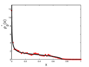
Figure 12: (Color online). Density of eigenvalues $x$ for $N=5$ and $p=5$ (theory vs. numerics) for $n=2$.

VI.2 Intermediate $p$: support on $(0,1)$

We now look for the solution of

$$n\frac{p}{2}x^{n-1}=\mathrm{Pr}\int_{0}^{1}\frac{\varrho_{p}^{\star}(x^{\prime})}{x-x^{\prime}}dx^{\prime}$$ (131)

with a nonzero support over the full allowed range $[0,1]$. Using the general solution in (31) with the choice $a=0$ and $b=1$ we get

$$\varrho_{p}^{\star}(x)=\frac{np\Gamma(n-1/2)}{4\Gamma(n+1)\pi^{3/2}}\left[\frac{~{}_{2}F_{1}(1,-n;3/2-n;x)-C_{n}}{\sqrt{x(1-x)}}\right]$$ (132)

where $C_{n}$ is an arbitrary constant to be fixed by $\int_{0}^{1}\varrho_{p}^{\star}(x)dx=1$, yielding:

$$C_{n}=-\frac{4\sqrt{\pi}\Gamma(n)}{p\Gamma(n-1/2)}$$ (133)

so eventually:

$$\varrho_{p}^{\star}(x)=\frac{p\Gamma(n-1/2)}{4\Gamma(n)\pi^{3/2}}\left[\frac{~{}_{2}F_{1}(1,-n;3/2-n;x)+\frac{4\sqrt{\pi}\Gamma(n)}{p\Gamma(n-1/2)}}{\sqrt{x(1-x)}}\right]$$ (134)

Next, we need to impose the condition (114):

$$t=\int_{0}^{1}dx~{}x^{n}\varrho_{p}^{\star}(x)$$ (135)

leading to:

$$t=\frac{\Gamma(n+1/2)}{\sqrt{\pi}\Gamma(n+1)}\left[1+\frac{p\Gamma(n-1/2)}{8\sqrt{\pi}\Gamma(n)}(1-2n)\right]$$ (136)

From (136) we can derive the relation between $p$ and $t$ as:

$$p=a_{n}-b_{n}t$$ (137)

where:

$$a_{n} =\frac{4\sqrt{\pi}\Gamma(n)}{\Gamma(n+1/2)}$$ (138)

$$b_{n} =\frac{4\pi\Gamma(n)\Gamma(n+1)}{[\Gamma(n+1/2)]^{2}}$$ (139)

Inserting (137) and (134) into (115), we obtain, after a few steps of algebra, the action:

$$S[\varrho_{p}^{\star}]=\frac{b_{n}}{2}\left[t-\frac{\Gamma(n+1/2)}{\sqrt{\pi}\Gamma(n+1)}\right]^{2}+\log 4$$ (140)

Next we need to determine the range of validity of this solution. This is obtained simply by the fact that the density $\varrho_{p}^{\star}(x)$ in (132) must be positive. Let us first rewrite the solution (132) as

$$\varrho_{p}^{\star}(x)=\frac{1}{\pi}\,\frac{A_{p}(x)}{\sqrt{x(1-x)}}$$ (141)

where

$$A_{p}(x)=1+\frac{p\Gamma(n-1/2)}{4\sqrt{\pi}\Gamma(n)}\,_{2}F_{1}(1,-n;3/2-n;x).$$ (142)

To ensure $\varrho_{p}^{\star}(x)\geq 0$, we have to just ensure that $A_{p}(x)\geq 0$ in (142). How does $A_{p}(x)$ vary as a function of $x$ in $x\in[0,1]$? It can be easily seen that this function has a global minimum at some intermediate value $0<x^{\star}<1$. To ensure its positivity, we then have to ensure that $A_{p}(x^{\star})\geq 0$. This will be true only for a range of values of $p$, i.e., when $p_{2}^{\star}\leq p\leq p_{1}^{\star}$ (where $p_{1}^{\star}$ is precisely the lower edge of the validity of regime I in the previous subsection and is given in (127)). Consequently, using (137), this sets a $t$ range $t_{1}^{\star}\leq t\leq t_{2}^{\star}$ for the validity of this regime II, where $t_{1}^{\star}$ is given in (128). Now, for arbitrary $n$, $p_{2}^{\star}$ and consequently $t_{2}^{\star}$ have rather complicated expressions which we do not detail here. But for $n=2$, their expressions are rather simple and we get

$$p_{2}^{\star}=-\frac{16}{3};\quad{\rm and}\quad t_{2}^{\star}=\frac{3}{4}$$ (143)

This then defines regime II with a full support over $[0,1]$, namely $-16/3\leq p\leq 8/3$ and consequently $3/16\leq t\leq 3/4$, is shown as the second (from the left) region in fig. 16.

Thus in this regime II where $t_{1}^{\star}\leq t_{2}^{\star}$, the rate function, for arbitrary $n$, has a quadratic form:

$$\Psi_{\mathcal{T}_{n}}(t)=S[\varrho_{p}^{\star}]-\log 4=\frac{b_{n}}{2}\left[t-\frac{\Gamma(n+1/2)}{\sqrt{\pi}\Gamma(n+1)}\right]^{2}$$ (144)

thus implying (13):

$$\mathcal{P}_{\mathcal{T}_{n}}(\mathcal{T}_{n},N)\approx\exp\left[-\frac{\beta}{2}N^{2}\frac{b_{n}}{2}\left[\frac{\mathcal{T}_{n}}{N}-\frac{\Gamma(n+1/2)}{\sqrt{\pi}\Gamma(n+1)}\right]^{2}\right]$$ (145)

In fig. 13 we plot the theoretical density of eigenvalues for the $n=2$ case together with Montecarlo simulations with $N=6$ and $p=1$.

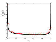
Figure 13: (Color online). Density of eigenvalues $x$ for $N=6$ and $p=1$ (theory vs. numerics) for $n=2$.

From the Gaussian shape in (145), the mean and variance of $\mathcal{T}_{n}$ can be read off very easily:

$$\langle\mathcal{T}_{n}\rangle =\frac{N\Gamma(n+1/2)}{\sqrt{\pi}\Gamma(n+1)}$$ (146)

$$\mathrm{var}(\mathcal{T}_{n}) =\frac{2}{\beta b_{n}}=\frac{[\Gamma(n+1/2)]^{2}}{2\beta\pi\Gamma(n)\Gamma(n+1)}$$ (147)

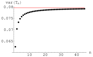
Figure 14: (Color online). $\mathrm{var}(\mathcal{T}_{n})$ as a function of $n\in\mathbb{N}$ (147) for $\beta=2$. In red the asymptotic value $v^{\star}=1/2\pi\beta\approx 0.07957$ (149).

Novaes [25] recently computed the average of integer moments and obtained the following expression for arbitray $n\in\mathbb{N}$:

$$\langle\mathcal{T}_{n}\rangle=N\binom{2n}{n}4^{-n}$$ (148)

Using elementary properties of Gamma functions, it is easy to show that formulae (146) and (148) do indeed coincide, a fact not completely apparent at first sight.

Conversely, the exact expression for the large $N$ variance (147) is new, since the general integral in Beenakker’s formula [29] does not appear easy to carry out explicitly. Obviously, (147) agrees with the known result [29] for the conductance $\mathrm{var}(G)=1/8\beta$ for $n=1$.

From (147), it is easy to extract the asymptotic value:

$$v^{\star}=\lim_{n\to\infty}\mathrm{var}(\mathcal{T}_{n})=\frac{1}{2\beta\pi}$$ (149)

which is plotted in fig. 14 for $\beta=2$ together with (147).

For general $n$, as one increases the value of $t$, so far we have seen two regimes: regime I ($0\leq t\leq t_{1}^{\star}$) with support over $[0,L_{p}]$ and then regime II ($t_{1}^{\star}\leq t\leq t_{2}^{\star}$) with support over the full range $[0,1]$. What happens when $t$ increases beyond $t_{2}^{\star}$? For arbitrary $n$, the analysis becomes rather cumbersome. So from now we restrict ourselves only to the case $n=2$ (which turns out already to be rather nontrivial). But at least for $n=2$ we are able to obtain a full picture and in the two subsections below we show that apart from regime I and regime II already discussed above, two further regimes appear as one increases $t$ beyond $t_{2}^{\star}$: regime III (for $t_{2}^{\star}\leq t\leq t_{3}^{\star}$) where the solution has a disconnected support with two connected components discussed in subsection VI.4 and regime IV (for $t_{3}^{\star}\leq t\leq 1$) where the solution again has a single support but on the other side of the box over $[M_{p},1]$. Since the solution in regime IV is simpler (single support), we will first discuss this case in the next subsection VI.3 and finally the more involved case of regime III (with a disconnected support) will be discussed in subsection VI.4.

VI.3 Support on $[M_{p},1)$ ($n=2$): regime IV

Focussing on the $n=2$ case, we now look for a solution of (118) with a single support $[M_{p},1]$ where $M_{p}$ is yet to be determined. Using the general single support Tricomi solution (31) choosing $a=M_{p}$ and $b=1$, one obtains the following explicit solution

$$\varrho_{p}^{\star}(x)=-\frac{1}{\pi^{2}\sqrt{(x-M_{p})(1-x)}}\left[p~{}\mathrm{Pr}\int_{M_{p}}^{1}\frac{\sqrt{(1-x^{\prime})(x^{\prime}-M_{p})}}{x-x^{\prime}}\,x^{\prime}\,dx^{\prime}+D\right]$$ (150)

where $D$ is an arbitrary constant. Evaluating the principal value integral in (150) and imposing $\varrho_{p}^{\star}(M_{p})=0$ we obtain

$$\varrho_{p}^{\star}(x)=\frac{-p(2x+M_{p}-1)}{2\pi}\sqrt{\frac{x-M_{p}}{1-x}}$$ (151)

The lower edge $M_{p}$ is determined by the normalization condition $\int_{M_{p}}^{1}\varrho_{p}^{\star}(x)dx=1$, yielding a quadratic equation for $M_{p}$: $p(M_{p}-1)(1+3M_{p})=8$ with two roots $M_{p}=(1\pm 2\sqrt{1+6/p})/3$. Noting that when $p\to-\infty$, it follows from physical consideration that the charge density must be pushed to its rightmost limit indicating that $M_{p}\to 1$ as $p\to-\infty$. This condition forces us to choose the correct root as

$$M_{p}=\frac{1}{3}\,\left(1+2\sqrt{1+\frac{6}{p}}\right).$$ (152)

The condition $0\leq M_{p}\leq 1$ implies for $p$ the condition $p\leq p_{3}^{\star}=-6$. The relation between $p$ and $t$ is then obtained using (114), resulting in the condition:

$$\frac{15+27M_{p}+13M_{p}^{2}+9M_{p}^{3}}{16(3M_{p}+1)}=t$$ (153)

where $M_{p}$ is expressed as a function of $p$ in (152). The solution of (153) is quite cumbersome to write down explicitly, but is in principle feasible. Note that when $p\to-6$ from below, $M_{p}\to 1/3$ from (152) and consequently from (153), $t\to t_{3}^{\star}=29/36$ from above. In other words, the solution (151) is valid in regime IV defined by

$$p\leq p_{3}^{\star}=-6;\quad{\rm consequently},\,\quad t_{3}^{\star}=\frac{29}{36}\leq t\leq 1$$ (154)

This regime IV is shown in the extreme right part of Fig. 16.

Once $p$ has been determined has a function of $t$ from (152) and (153) and substituted into the density (151), the action and the rate function can be computed from (115) and (117), by evaluating numerically the corresponding integrals. We omit these details here.

In fig. 15 we plot the theoretical density of eigenvalues for the $n=2$ case together with Montecarlo simulations with $N=4$ and $p=-10$.

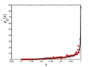
Figure 15: (Color online). Density of eigenvalues $x$ for $N=4$ and $p=-10$ (theory vs. numerics) for $n=2$.

VI.4 Disconnected support ($n=2$): regime III

For $n=2$, it then remains to find the solution of (118) in the narrow band $t_{2}^{\star}=3/4\leq t\leq t_{3}^{\star}=29/36$ or equivalently for $p_{3}^{\star}=-6\leq p\leq p_{2}^{\star}=-16/3$ (see Fig. 16). This is the regime III. Let us first try to anticipate what the solution may look like in this regime. For this, let us consider the two regimes namely regime II and regime IV respectively to the left and right of regime III.

Consider first regime II ($t_{1}^{\star}=3/16\leq t\leq t_{2}^{\star}=3/4$). In this regime the solution $\varrho_{p}^{\star}(x)$ has a single support over the full range $x\in[0,1]$ given in (134), which for $n=2$ (using the special value of the hypergeometric function) simply reads, with $p_{2}^{\star}=-16/3\leq p\leq p_{1}^{\star}=8/3$,

$$\varrho_{p}^{\star}(x)=\frac{1}{\pi\sqrt{x(1-x)}}\left[1+\frac{p}{8}(1+4x-8x^{2})\right].$$ (155)

Now, when $t$ tends to the maximum allowed value in regime II, namely, $t\to t_{2}^{\star}=3/4$ from below or equivalently $p\to p_{2}^{\star}=-16/3$ from above, the solution in (155) tends to

$$\varrho_{-16/3}^{\star}(x)=\frac{16}{3\pi\sqrt{x(1-x)}}\,\left[x-\frac{1}{4}\right]^{2}$$ (156)

with a quadratic minimum at $x=1/4$ where the density vanishes. This is just the edge of regime II. If $t$ increases slightly beyond $t_{2}^{\star}=3/4$, this single support solution is no longer valid. However, it gives the hint that for $t>t_{2}^{\star}=3/4$, the charge density must separate into two disjoint components, one on the left side over $[0,l_{1}]$ and one on the right side over $[l_{2},1]$ with an empty stretch $[l_{1},l_{2}]$ separating them. This empty stretch must increase as one increases $t$ beyond $t_{2}^{\star}=3/4$ in this regime III. Indeed, as $t$ increases further, the left support $[0,l_{1}]$ must shrink in size and the right support $[l_{2},1]$ must increase in size and finally when $t$ hits the value $t_{3}^{\star}=29/36$, $l_{1}$ must shrink to $0$ and $l_{2}$ must approach $M_{p}=1/3$ and then one arrives in regime IV discussed in the previous subsection. At exactly $t=t_{3}^{\star}=29/36$ or equivalently at $p=p_{3}^{\star}=-6$, the solution (border of regime IV) can be read off (151) with $M_{p}=1/3$

$$\varrho_{-6}^{\star}(x)=\frac{6}{\pi\sqrt{1-x}}\,\left(x-\frac{1}{3}\right)^{3/2}.$$ (157)

Thus, the solution in regime III, namely for $p_{3}^{\star}=-6\leq p\leq p_{2}^{\star}=-16/3$ must interpolate between the solutions given in (156) and in (157) valid respectively at the two edges of regime III and have a disconnected support with two connected components over $[0,l_{1}]$ and $[l_{2},1]$. We were able to find this solution explicitly. Its derivation is outlined in the Appendix. The result reads

$$\varrho_{p}^{\star}(x)=\frac{-p}{\pi\sqrt{x(1-x)}}\,\sqrt{(x-l_{1})(x-l_{2})^{3}}$$ (158)

which is valid for all $0\leq x\leq l_{1}$ and $l_{2}\leq x\leq 1$ and the two edges $l_{1}$ and $l_{2}$ are given by

$$l_{1} = \frac{1}{4}\left(1-3\sqrt{1+\frac{16}{3p}}\right)$$ (159)

$$l_{2} = \frac{1}{4}\left(1+\sqrt{1+\frac{16}{3p}}\right)$$ (160)

Note that $l_{1}$ and $l_{2}$ are real only if $p\leq-16/3$. Furthermore $l_{1}\geq 0$ only if $p\geq-6$. Thus this solution is valid over the full range $p_{3}^{\star}=-6\leq p\leq p_{2}^{\star}=-16/3$. This then defines regime III. Note also that the solution (158) smoothly interpolates between the solutions in (156) (when $p\to-16/3$) and in (157) (when $p\to-6$).

The relation between $t$ and $p$ can be obtained substituting (158) in (114) and performing the integral. Similarly the action and the rate function can be computed by using the exact density and performing the integrals in (115) and (117) by Mathematica, the details of which we omit here. The Montecarlo simulations in this regimes are much harder to obtain due to large fluctuations in sampling from the leftmost residual band $0\leq x\leq l_{1}$ and a very large $N$ is necessary to achieve a satisfactory picture. Nevertheless, we observed upon increasing $N$ a trend in the equilibrium density which is fully compatible with the analytical disconnected-support solution found above.

VI.5 Final results for the $n=2$ moment case

In fig. 16 we propose a schematic summary of the different phases of the density of integer moments for the case $n=2$. As a consequence, the rate function will display three (and not just two, as for conductance and shot noise) non-analytical points corresponding to physical phase transitions in Laplace space. Starting from high $p$ values, the fluid particles are initially confined towards the left hard edge. Then, when $p$ hits the critical value $p=8/3$, the fluid spreads over the entire support $[0,1]$. In the narrow region $-6\leq p\leq-16/3$ the density splits over two disjoint (non-symmetric) components of the support, and the leftmost disappears upon hitting the value $p=-6$, leaving the charges leaning against the right hard wall.

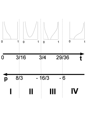
Figure 16: Schematic table summarizing the relevant phases in the $t$ and $p$ space for the density of $n=2$ moment. As $t$ varies in the allowed range $[0,1]$ and consequently the parameter $p$ in $[-\infty,\infty]$, the fluid density displays 4 different phases as shown in the top panel. These $4$ regimes are separated by three critical points: $t_{1}^{\star}=3/16$ (consequently $p_{1}^{\star}=8/3$), $t_{2}^{\star}=3/4$ ($p_{2}^{\star}=-16/3$) and $t_{3}^{\star}=29/36$ ($p_{3}^{\star}=-6$). Consequently, the rate function $\Psi_{\mathcal{T}_{n}}(t)$ has 4 different expressions according to different regions in the $t\in[0,1]$ segment.

VII Conclusions

The Coulomb gas analogy, together with recently introduced functional methods, brings about an efficient formalism for the computation of full probability distributions of observables (valid for a large number of electronic channels in the two leads) in the quantum conductance problem. Generically, the distribution of any linear statistics of the form $A=\sum_{i=1}^{N}a(T_{i})$, where the $T_{i}$’s are transmission eigenvalues of the cavity and $a(x)$ is any smooth function, can be derived within the formalism described in this paper: the problem amounts to finding the equilibrium configuration of an associated 2d charged fluid confined to the segment $[0,1]$ and subject to two competing interactions: the logarithmic repulsion, generated by the Vandermonde term in the jpd (2), and a confining potential whose strength is tuned by the Laplace parameter $p$. Interestingly, this auxiliary Coulomb gas undergoes different phase transitions as the Laplace parameter is varied continuously, and this physical picture is mirrored in the appearance of very weak singularities in the rate functions of observables at the critical points. Already the leading $N$-term of the free energy of such a gas (the spherical contribution) displays non-Gaussian features in the tails, while the central region obeys the Gaussian law, in agreement with the general Politzer’s argument [59]; conversely the tails follow a power-law decay and the junctions of the two (or more, as in the case of integer moments) regimes are continuous but non-analytical points. Note that it is not necessary to develop a $(1/N)$ expansion of the free energy and look for higher genus terms to appreciate deviations from the Gaussian law. From the central Gaussian region, one can easily reads off the mean and variance of any linear statistics of interest: this way well known results for e.g. conductance and shot noise are recovered and new formulas (such as the variance of integer moments and its universal asymptotics) can be derived. Our results are well-corroborated by Montecarlo simulations both in the real and Laplace space, as well as by comparison with exact finite $N$ results when available, which convincingly disprove the large-$N$ asymptotic analysis performed in [39]. In summary, the Coulomb gas method (well-suited to large $N$ evaluations) reveals a rich thermodynamic behavior for the quantum conductance problem already at the leading order level, and we expect that it will enjoy a broad range of applicability.

Appendix A Explicit Two Support Solution for $n=2$ in Regime III

We consider the integral equation (118) for $n=2$

$$px=\mathrm{Pr}\int_{0}^{1}\frac{\varrho_{p}^{\star}(x^{\prime})dx^{\prime}}{x-x^{\prime}}$$ (161)

and look for a solution that has a disconnected support with two connected components ($[0,l_{1}]$ and $[l_{2},1]$). This solution is valid in regime III discussed in subsection VI-D. While a general single support solution of the singular integral equation can be found using Tricomi’s formula given in (31) with $g(x)=px$ and discussed in subsections VI-A, VI-B and and VI-C, it is much more complicated to obtain an explicit solution with more than one connected component of the support. To find such a solution, we actually use an alternative method originally used by Brezin et. al. to find a single support solution of the singular integral equation in the context of counting of planar diagrams [60]. This method consists in making a judicious guess for the solution and then uses the uniqueness properties of analytic functions in a complex plane to prove that the guess is right. Although, for the single support solution one does not have to use this route since the explicit general solution of Tricomi is available ( the authors of ref. [60] were perhaps unaware of the general single support explicit solution of Tricomi). Nevertheless, this alternative method of  [60] can be fruitfully adapted to find a two support solution (as in our case) in a simpler way (as demonstrated below), where a general solution is somewhat difficult to obtain explicitly.

Let us assume that the solution $\varrho_{p}^{\star}(x)$ of (161) has a disconnected support with two connected components $[0,l_{1}]$ and $[l_{2},1]$ where $l_{1}$ and $l_{2}\geq l_{1}$ are yet to be determined. Generalizing the route used for single support solution in ref. [60], we first introduce an analytic function (without the principal part in (161))

$$F(x)=\int_{0}^{l_{1}}\frac{\varrho_{p}^{\star}(x^{\prime})dx^{\prime}}{x-x^{\prime}}+\int_{l_{2}}^{1}\frac{\varrho_{p}^{\star}(x^{\prime})dx^{\prime}}{x-x^{\prime}}$$ (162)

defined everywhere in the complex $x$ plane outside the two real intervals $[0,l_{1}]$ and $[l_{2},1]$. This new function $F(x)$ has the following properties:

1. it is analytic in the complex $x$ plane outside the two cuts $[0,l_{1}]$ and $[l_{2},1]$,

2. it behaves as $1/x$ when $|x|\to\infty$ since $\int\varrho_{p}^{\star}(x^{\prime})dx^{\prime}=1$ due to normalization,

3. it is real for $x$ real outside the two cuts $[0,l_{1}]$ and $[l_{2},1]$,

4. as one approaches to any point $x$ on the two cuts $[0,l_{1}]$ and $[l_{2},1]$ on the real axis, $F(x\pm i\epsilon)=px\mp i\pi\varrho_{p}^{\star}(x)$. This last property follows from (161).

From the general properties of analytic functions in the complex plane it follows that there is a unique function $F(x)$ which satisfies all the four properties mentioned above. Thus, if one can make a good guess for $F(x)$ and one verifies that it satisfies all the above properties, then this $F(x)$ is unique. Knowing $F(x)$, one can then read off the solution $\varrho_{p}^{\star}(x)$ from the $4$-th property. It then rests to make a good guess for $F(x)$. We try the following ansatz for $F(x)$ valid everywhere outside the two cuts $[0,l_{1}]$ and $[l_{2},1]$

$$F(x)=px-\frac{p}{\sqrt{x(x-1)}}\sqrt{(x-l_{1})(x-l_{2})^{3}}.$$ (163)

This ansatz clearly satisfies the first property. Now, expanding $F(x)$ for large $|x|$ we get

$$F(x) \to(-1+l_{1}+3l_{2})p+$$

$$+\frac{p}{8}(-3+2l_{1}+l_{1}^{2}+6l_{2}-6l_{1}l_{2}-3l_{2}^{2})\,\frac{1}{x}+O(x^{-2})$$ (164)

Since the second property dictates that $F(x)\to 1/x$, it follows that we must have

$$l_{1}+3l_{2}=1$$ (165)

$$(-3+2l_{1}+l_{1}^{2}+6l_{2}-6l_{1}l_{2}-3l_{2}^{2})=8$$ (166)

Eliminating $l_{2}$ in (166) using (165) gives a quadratic equation for $l_{1}$, $2l_{1}^{2}-l_{1}-1=6/p$ with two solutions: $l_{1}=(1\pm 3\sqrt{16/p})/4$. The correct root is chosen by the fact that when $p\to-6$, $l_{1}\to 0$ as follows from the solution in (157). This then uniquely fixes $l_{1}$ and $l_{2}$ given respectively in (159) and (160).

The ansatz $F(x)$, with the choices $l_{1}$ and $l_{2}$ as in (159) and (160) then satisfies the second property. It is easy to check that $F(x)$ satisfies the third property as well. From the fourth property one then reads off the unique solution as given in (158). This two support solution is clearly valid only in the regime III namely for $p_{3}^{\star}=-6\leq p\leq p_{2}^{\star}=-16/3$ and it smoothly matches with the solutions of regime II and regime IV respectively as $p\to-16/3$ and $p\to-6$.