Micro- and macroturbulence derived from 3D hydrodynamical stellar atmospheres

Abstract

The theoretical prediction of micro- and macroturbulence ($\xi_{\rm mic}$ and $\xi_{\rm mac}$) as a function of stellar parameters can be useful for spectroscopic work based on 1D model atmospheres in cases where an empirical determination of $\xi_{\rm mic}$ is impossible due to a lack of suitable lines and/or macroturbulence and rotational line broadening are difficult to separate. In an effort to exploit the CIFIST 3D model atmosphere grid for deriving the theoretical dependence of $\xi_{\rm mic}$ and $\xi_{\rm mac}$ on effective temperature, gravity, and metallicity, we discuss different methods to derive $\xi_{\rm mic}$ from the numerical simulations, and report first results for the Sun and Procyon. In both cases the preliminary analysis indicates that the microturbulence found in the simulations is significantly lower than in the real stellar atmospheres.

1 Introduction

3D hydrodynamical simulations of stellar surface convection provide a physically self-consistent description of the non-thermal velocity field generated by convection, overshoot, and waves. This is one of the great advantages over classical 1D model atmospheres where the properties of the photospheric velocity field need to be specified empirically in terms of the free parameters $\xi_{\rm mic}$ and $\xi_{\rm mac}$. Even if these parameters are irrelevant in the context of 3D hydrodynamical model atmospheres, the latter may be used to predict the magnitude of $\xi_{\rm mic}$ and $\xi_{\rm mac}$ as a function of the stellar parameters ($T_{\rm eff}$, log g, [M/H]). The CIFIST 3D model atmosphere grid (Ludwig et al., this volume) provides a suitable database for this purpose. In the following, we investigate different methods to derive the parameter $\xi_{\rm mic}$ (and subsequently $\xi_{\rm mac}$) from our 3D model atmospheres which were computed with the CO⁵BOLD code (Freytag, Steffen, & Dorch, 2002; Wedemeyer et al., 2004). The Sun ($T_{\rm eff}$=5780 K, log g=4.44, [M/H]=0) and Procyon ($T_{\rm eff}$=6500 K, log g=4.0, [M/H]=0) serve as benchmarks for the present study.

2 Methods to derive $\xi_{\rm mic}$ and $\xi_{\rm mac}$

All methods described below presume that the photospheric velocity field may be characterized by a single, depth-independent value of $\xi_{\rm mic}$ and $\xi_{\rm mac}$, and that both micro- and macroturbulence have an isotropic Gaussian probability distribution of the line-of-sight velocity, $P(v)\sim\exp(-v^{2}/\xi^{2})$. Synthetic spectral lines serve as a diagnostic tool to probe $\xi_{\rm mic}$ and  $\xi_{\rm mac}$ via the total absorption (equivalent width $W$) and the shape of the line, respectively.

Method 1 (M1) is considered the most accurate procedure to extract the microturbulence parameter from a 3D numerical convection simulation. Unlike the other methods described below, it relies only on the 3D model, and yields a value of $\xi_{\rm mic}$ for any individual spectral line, thus allowing to map $\xi_{\rm mic}(W)$. Given the spectral line parameters, the line profile is computed from the 3D model with different velocity fields: (i) using the original 3D hydrodynamical velocity field, and (ii) replacing the 3D hydrodynamical velocity field by an isotropic, depth-independent microturbulence, like in classical 1D spectrum synthesis, but retaining the full 3D thermodynamic structure. Now the microturbulence associated with the considered spectral line, $\xi^{(1)}_{\rm mic}$, is defined by the requirement of matching line strengths: $W_{\rm 3D}({\rm hydro})=W_{\rm 3D}(\,\xi^{(1)}_{\rm mic})$, where $W_{\rm 3D}({\rm hydro})$ and $W_{\rm 3D}(\,\xi_{\rm mic})$ are the equivalent widths obtained in steps (i) and (ii), respectively.

Once $\xi_{\rm mic}$ is determined as explained above, the macroturbulence associated with the considered spectral line is defined by minimizing the mean square difference between the 3D line profile computed in step (i) with the hydrodynamical velocity field, and the modified 3D line profile obtained in step (ii) with $\xi^{(1)}_{\rm mic}$ and subsequent convolution with the macroturbulence velocity dispersion ($\xi_{\rm mac}$). The IDL procedure MPFIT is used to find the solution $\xi^{(1)}_{\rm mac}$ that gives the best fit to the original 3D profile.

Method 2a/b (M2a/b) The idea of this method is to replace the modified 3D models (furnished with a classical microturbulence velocity field) used in step (ii) of Method 1 with an arbitrary 1D model atmosphere. However, this concept does not work for a single spectral line, but instead has to rely on a set of spectral lines ranging from weak to partly saturated. In Method 2 the set of lines is generated from a curve-of-growth, i.e. all lines share the same atomic parameters except for the $f$-value, which controls the line strength. Given the set of fictitious spectral lines and a 1D model atmosphere, we first compute for each line $i$ the 1D-3D abundance difference $\Delta\log\epsilon_{i}(\,\xi_{\rm mic})$, defined by the condition $W_{\rm 3D}\,(\log gf_{i})=W_{\rm 1D}\,(\xi_{\rm mic},\log gf_{i}+\Delta\log\epsilon_{i})$, i.e. $\Delta\log\epsilon_{i}$ is the logarithmic abundance difference between the abundance derived from the 1D model by fitting the equivalent of the 3D profile, and the true abundance assumed in computing the 3D spectral line. In M2a we compute the slope of the linear regression to the data set $\{W_{\rm 3D},\;\Delta\log\epsilon_{i}(\,\xi_{\rm mic})\}$, and define $\xi^{(2a)}_{\rm mic}$ by the condition of vanishing slope, $\beta(\,\xi^{(2a)}_{\rm mic})=0$. Alternatively, in M2b the microturbulence is required to produce the minimum standard deviation of {$\Delta\log\epsilon_{i}$}, $\sigma(\,\xi^{(2b)}_{\rm mic})$ = $\min$. Once $\xi_{\rm mic}$ is determined, the macroturbulence associated with each individual spectral line, $\xi^{(2)}_{\rm mac}$, is found by fitting the original 3D line profile with the corresponding 1D line profile (with fixed $\xi^{(2)}_{\rm mic}$) through variation of $\xi_{\rm mac}$, in essentially the same way as in Method 1.

Method 3a/b (M3a/b) is very similar to Method 2, except for utilizing a sample of real spectral lines of different strength (and different wavelength, excitation potential, etc.) instead of a set of fictitious lines lying on a single curve-of-growth. Adjusting the value of $\xi_{\rm mic}$ to minimize the difference in $\Delta\log\epsilon_{i}$ between weak and strong lines obtained from the preferred 1D model results in $\xi^{(3a)}_{\rm mic}$ (zero slope condition). Similarly, minimizing the overall dispersion of $\Delta\log\epsilon_{i}$ gives $\xi^{(3b)}_{\rm mic}$. Method 3 corresponds to the classical definition of $\xi_{\rm mic}$. Again $\xi^{(3)}_{\rm mac}$ is found as in Method 2.

Note that all 3 methods have the advantage that errors in $\log gf$ cancel out. Only Method 3 can also be applied to observed stellar spectra; in this case the accuracy of the $\log gf$ values is crucial. Obviously, the results depend on the selected spectral lines, and, for Methods 2 and 3, on the choice of the 1D model atmosphere.

In principle, it should be possible to derive $\xi_{\rm mic}$ and $\xi_{\rm mac}$ directly from evaluating the 3D hydrodynamical velocity field without resorting to synthetic spectral lines. But a suitable procedure (Method 4) has yet to be developed.

3 First results: Sun and Procyon

Figures 1 and 2 show the determination of the microturbulence parameter from a 3D model atmosphere of the Sun and Procyon, respectively, according to the three methods described above. We considered 5 sets of fictitious iron lines (Fe I 0, and 5 eV, Fe II 0, 5, and 10 eV, used with M1, M2), and one sample of real Fe I and Fe II lines each (used with M1, M3). The most obvious result is that the microturbulence derived from the flux spectra is systematically higher than that obtained from the intensity spectra, in agreement with observational evidence (e.g. Holweger et al., 1978). Moreover, the derived value of $\xi_{\rm mic}$ depends on the type and strength of the considered spectral line. Method 1 clearly reveals that high-excitation lines ‘feel’ a lower microturbulence than low-excitation lines. The dependence of $\xi_{\rm mic}$ on line strength is non-trivial (see Fig. 1, lower panel). In general, Methods 2a and 2b give very similar results, which moreover agree well with the results obtained from Method 1 for the stronger lines on the curve-of-growth. In contrast, Methods 3a and 3b can give rather discordant answers, if the sample of spectral lines is not sufficiently homogeneous (see again lower panel of Fig. 1).

In Table 1, the theoretical predictions of micro- and macroturbulence based on our hydrodynamical model atmospheres for the Sun and Procyon are summarized and confronted with empirical results from the literature. This preliminary analysis indicates that the theoretical predictions of $\xi_{\rm mic}$ fall significantly below the classical empirical estimates, for both solar intensity and flux spectra, and even more clearly for Procyon, as demonstrated unmistakably in Fig. 3. On the other hand, the macroturbulence derived from the CO⁵BOLD models is somewhat larger than deduced from observations, such that the total non-thermal rms velocity $v_{\rm turb}$ (columns (6) and (7) of Tab. 1), and hence the total line broadening, is very similar in simulations and observations.

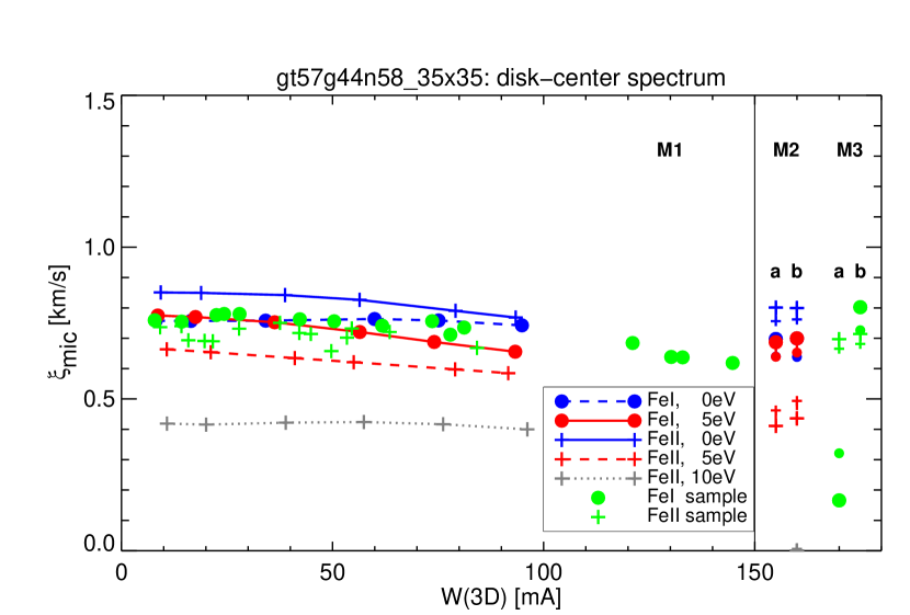
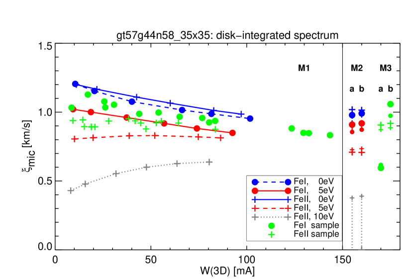
Figure 1: Overview of $\xi_{\rm mic}$ derived from our standard 3D solar model atmosphere (gt57g44n58) determined with M1, M2, and M3 for a total of 60 different Fe I (filled circles) and Fe II (plus signs) lines. Connected symbols represent fictitious lines sharing the same curve-of-growth, individual symbols indicate real spectral lines. The results of M2a,b (red, blue) and M3a,b (green) are shown to the right of the vertical line in each panel for two different 1D models (smaller symbols: $\langle$3D$\rangle$, larger symbols: HM). Top and bottom panels refer to disk-center and full-disk spectra, respectively.

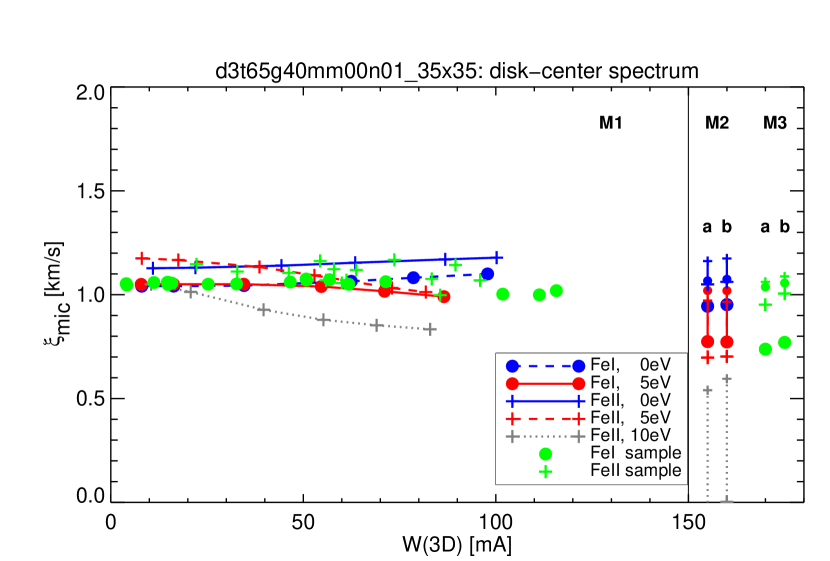
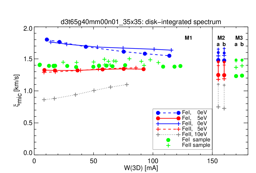
Figure 2: As Fig. 1, but for a 3D model atmosphere representative of Procyon, using a total of 56 different Fe I (filled circles) and Fe II (plus signs) lines. 1D models used with M2, M3: $\langle$3D$\rangle$ (smaller symbols) and LHD [$\alpha_{\rm MLT}$=$0.5$] (larger symbols). Top and bottom panels refer to disk-center and full-disk spectra, respectively.

Table 1: Empirical values of $\xi_{\rm mic}$ and $\xi_{\rm mac}$ from the literature, compared with the theoretical results derived in this work from 3D CO⁵BOLD hydrodynamical model atmospheres for the Sun and Procyon (weighted average over Methods 1, 2 and 3).

Atmosphere /	$\xi_{\rm mic}$ [km/s]		$\xi_{\rm mac}$ [km/s]		$v_{\rm turb}=\sqrt{(\xi_{\rm mic}^{2}+\xi_{\rm mac}^{2})/2}$  [km/s]
Model	disk-center	full-disk	disk-center	full-disk	disk-center	full-disk
Sun, observed${}^{\,a}$	$1.00\pm 0.15$	$1.35\pm 0.15$	$1.63\pm 0.15$	$1.90\pm 0.15$	$1.35\pm 0.10$	$1.65\pm 0.10$
3D solar model	$0.70\pm 0.10$	$0.95\pm 0.15$	$1.85\pm 0.45$	$2.30\pm 0.30$	$1.40\pm 0.30$	$1.75\pm 0.20$
(gt57g44n58)
Procyon, observed${}^{\,b}$	—	$2.10\pm 0.30$	—	$4.20\pm 0.50$	—	$3.30\pm 0.30$
3D Procyon model	$0.95\pm 0.25$	$1.45\pm 0.25$	$3.10\pm 0.40$	$4.45\pm 0.20$	$2.30\pm 0.30$	$3.30\pm 0.15$
(d3t65g40mm00n01)

Notes: a: Holweger et al. (1978), full-disk values interpolated: $\xi^{2}$(full-disk)=$\xi^{2}$(disk-center)/2 + $\xi^{2}$(limb)/2;
b: Steffen (1985)

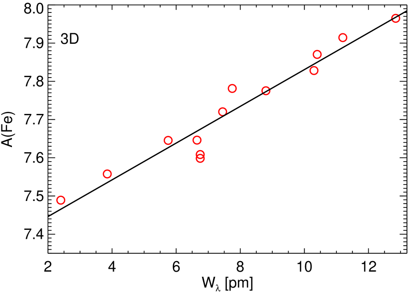
Figure 3: Iron abundance derived from individual Fe II lines using a 3D CO⁵BOLD model with $T_{\rm eff}$=6500 K, log g=4.0, [M/H]=0, with log $gf$ values taken from Melendez & Barbuy (2009), and van der Waals line broadening treated according to Barklem et al. (1998). The strong trend of abundance with equivalent width indicates an apparent lack of small-scale turbulence in the hydrodynamical velocity field of the Procyon model.

4 Conclusions

We have developed different methods to extract the parameters $\xi_{\rm mic}$ and $\xi_{\rm mac}$ from 3D hydrodynamical simulations, and found all methods to give consistent results. As expected, $\xi_{\rm mic}$ and $\xi_{\rm mac}$ depend systematically on the properties of the selected spectral lines. Our preliminary analysis based on state-of-the-art CO⁵BOLD models for the Sun and Procyon indicates that the microturbulence seen in the simulations is significantly lower than measured in the real stars. This suggests that the velocity field provided by the current 3D hydrodynamical models is less ‘turbulent’ than it is in reality. It seems that the simulations predict essentially the correct total rms velocity, while underestimating the small-scale and overestimating the large-scale fluctuations. If confirmed, this deficiency implies a systematic overestimation of 3D abundances from stronger lines. Apparently, our findings are in conflict with the conclusions by Asplund et al. (2000). Further investigations are necessary to find the basic cause of this disagreement and to clarify possible implications for high-precision abundance studies.

References

- Asplund et al. (2000) Asplund, M., Nordlund, Å., Trampedach, R., Allende Prieto, C., & Stein, R. F. 2000, A&A, 359, 729
- Barklem et al. (1998) Barklem, P. S., Anstee, S. D., & O’Mara, B. J. 1998, PASA, 15, 336
- Freytag, Steffen, & Dorch (2002) Freytag, B., Steffen, M., & Dorch, B. 2002, AN, 323, 213
- Holweger et al. (1978) Holweger, H., Gehlsen, M., & Ruland, F. 1978, A&A, 70, 537
- Melendez & Barbuy (2009) Melèndez, J., & Barbuy, B. 2009, A&A, 497, 611
- Steffen (1985) Steffen, M. 1985, A&AS, 59, 403
- Wedemeyer et al. (2004) Wedemeyer, S., Freytag, B., Steffen, M., Ludwig, H.-G., & Holweger, H. 2004, A&A, 414, 1121