Quantum Probability Explanations for Probability Judgment ‘Errors’

Abstract

A quantum probability model is introduced and used to explain human probability judgment errors including the conjunction, disjunction, inverse, and conditional fallacies, as well as unpacking effects and partitioning effects. Quantum probability theory is a general and coherent theory based on a set of (von Neumann) axioms which relax some of the constraints underlying classic (Kolmogorov) probability theory. The quantum model is compared and contrasted with other competing explanations for these judgment errors including the representativeness heuristic, the averaging model, and a memory retrieval model for probability judgments. The quantum model also provides ways to extend Bayesian, fuzzy set, and fuzzy trace theories. We conclude that quantum information processing principles provide a viable and promising new way to understand human judgment and reasoning.

Over 30 years ago, Kahneman and Tversky [1] began their influential program of research to discover the heuristics and biases that form the basis of human probability judgments. Since that time, a great deal of new and challenging empirical phenomena have been discovered including conjunction, disjunction, conditional, inverse, and base rate fallacies [2]. Although heuristic concepts (such as representativeness and availability) initially served as a guide to researchers in this area, there is a growing need to move beyond these intuitions, and develop more coherent, comprehensive, and deductive theoretical explanations [3]. The purpose of this article is to propose a new way of understanding human probability judgment using quantum probability principles [4].  Quantum principles have been used recently in a number of psychological applications including perception [5], conceptual structure [6], information retrieval [7], and human judgments [8].

The concept of a probability judgment error requires a standard or norm, and in the past, this norm was based on the Kolmogorov axioms for classic probability theory [11]. Classic theory is based on the assignment of probabilities to events defined as sets, and the Boolean logic entailed by using sets seems to be the source of the problems that occur with applications to human judgments. Quantum probability provides a more general geometric approach to probability theory that remains coherent but relaxes some of the constraints of Boolean logic [12]. Thus quantum probability provides an opportunity to explain what appears to be judgmental ‘errors’ with respect to the classic definition, but at the same time, it provides a quantum logical ‘rationale’ for human probability judgments.

The remainder of this article is organized as follows. First we provide some background information and review basic findings. Second, we provide a simple and elementary introduction to quantum probability theory and apply these ideas to the basic findings. Finally, we summarize previous theoretical explanations, compare the advantages and disadvantages of the quantum model with the previous models, and indicate directions for future research.

1 Background and Brief Review

This article is mainly concerned with the explanation of conjunction and disjunction fallacies, and so the following review and later theoretical analyses focus on these two basic issues. However, it is important to briefly examine how well this explanation extends to some closely related phenomena, including conditional and inverse fallacies and ‘unpacking’ effects. Therefore, although we focus on conjunction and disjunction fallacies, we also briefly examine some closely related fallacies. This review addresses the many qualitative (ordinal level) findings that have been discovered over the past 30 years.

In many probability judgment studies, a story is provided which is followed by questions about the likelihood of events related to the story (e.g., a story about a liberal philosophy student from Berkeley named Linda is presented, and questions are asked about her future activities). Sometimes very little story is needed (e.g. a time and a place) and there is simply a causal connection between story events (e.g., an increase in cigarette tax is passed, and then a decrease in teenage smoking occurs). Some of the key experimental factors that are manipulated in these studies include the following. Questions about events can be related by referring to the same person (e.g., ‘Linda is a bank teller’, ‘Linda is active in feminist movement’) or unrelated by referring to different people (‘Linda is active in feminist movement’, ‘Bill is shy’).  Questions about events can have high likelihood (e.g., ‘Linda is active in feminist movement’) or a low likelihood (‘Linda is a bank teller’).  Questions can be about events with positive (e.g., ‘Bill enjoys jogging and Bill plays soccer ’) or negative or zero dependencies (e.g., Bill is an accountant and Bill likes jogging’).

Questions about generic events are labeled by letters such as $A$ and $B$. We use the letters $H$ and $L$ to denote questions about events that have a high or low likelihood, respectively. Sometimes, subscripts on the letters will be used to distinguish questions about events that are related or unrelated. For example, $A_{1}$ and $B_{1}$ refer to events that are related (e.g., Tei has blue eyes, Tei has blond hair); $A_{1}$ and $B_{2}$ refer to events that are unrelated (e.g., Tei has blue eyes, Jerry has blond hair). When no subscripts appear, it can be assumed that the events are related. The probabilities of interest include questions about a single event (e.g., ‘is a $A$ true?’), a negation of a question (‘is not $A$ true?’ symbolized as $\char 126\relax A),$ a conjunctive question about events (‘is $A$ and $B$ true?’ symbolized $A\wedge B$), a disjunctive question about events (‘is $A$ or $B$ true?’ symbolized $A\vee B$), and a question about an implication (‘if $A$ is true, then is $B$ true?’, symbolized as $A\mapsto B$). The symbols $\wedge$ and $\vee$ represent the classic Boolean logic conjunction and disjunction relations, which are commutative, $(A\wedge B)\leftrightarrow(B\wedge A)$ and $(A\vee B)\leftrightarrow(B\vee A)$ and distributive $A\wedge(B\vee\char 126\relax B)\leftrightarrow(A\wedge B)\vee(A\wedge\char 126\relax B).$ The implication is not commutative $(A\mapsto B)\nleftrightarrow(B\mapsto A).$ These logical properties are intended by the experimenter asking the questions, but they may not necessarily be treated this way by human judges when answering questions about these events. Later, when various theoretical explanations for the findings are presented, different symbols are used for negation, conjunction, disjunction, and implication, because the formal properties of these logical relations differ across theories.

Participants are asked to judge probabilities for questions about events, and these judgments are denoted by the letter $J$. The judged probabilities corresponding to the single, negation, conjunction, union, and implication questions about events are denoted $J(A)\,$, $J(\char 126\relax A),$ $J(A\wedge B)$, $J(A\vee B)$, and $J(A\mapsto B)$. These judgments may be obtained using a choice response (e.g. which event is more likely), or rank ordering the likelihood of a list of events, or rating each event (e.g. what are the chances out of 100 that an event is true), and sometimes they are inferred from bets (e.g. decide which event you want to bet money). To evaluate whether or not a fallacy or judgment error occurs, one needs to compare the distribution of judgments across participants for one event with another. This is usually done using two methods: One is to compare the means (or medians) of the two distributions and determine whether the difference is statistically significant; the second is to compare the frequency of the correct versus incorrect orders and determine whether the frequencies are statistically different. These two methods usually but not always give the same answer when they are both reported.

1.1 Basic Findings

As mentioned earlier, this article is primarily concerned with conjunction and disjunction fallacies and some other closely related fallacies.  Figure 1 provides a general overview of (a) the magnitude of conjunction errors [14] in the top panel and (b) the magnitude of disjunction errors [15] in the bottom panel.

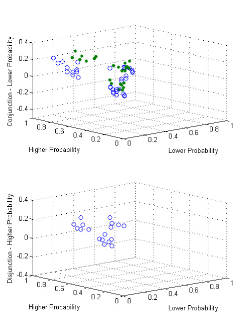
Figure 1: Top panel shows the mean conjunction effect from 60 experimental conditions, and bottom panel shows mean disjunction effect from 18 experimental conditions.

This figure plots the means of $J(H)$ and $J(L)$ along the X,Y axes, and the Z (vertical) axis has the mean of $J(H\wedge L)-J(L)$ for the conjunction error and the mean of $J(H)-J(H\vee L)$ for the disjunction error. The 36 open circles ($N=40$ observations per circle) in the top panel are from Table 1 of Gavansky & Roskos-Ewoldsen (1991) in which people judged the conjunction after the constituents; the 24 solid dots ($N=50$ observations per dot) in the top panel are from Table 2 of Gavansky and Roskos-Ewoldsen (1991) in which people judged the conjunction before the constituents, and the 18 circles ($N=88$ observations per circle) are from Experiment 2 of Fisk (2002) in which people judged the disjunction and the constituents in a randomized order. Points that lie above zero on the Z-axis indicate an error for the means. When the conjunction was rated last, five large (greater than .10) conjunction errors occurred and they all occurred for $J(L)<.3$ and $J(H)>.8$; when the conjunction was rated first, 7 large (greater than .10) conjunction errors occurred, and they all occurred for $J(L)<.40$ and $J(H)>.70$; 8 large (greater than .10) disjunction errors occurred, and all but two occurred for $J(L)<.30$ and $J(H)>.60$. In summary, large mean conjunctive and disjunctive errors tend to occur with a high-low combination, they tend to disappear when $J(L)$ is approximately equal to $J(H)$, and more errors occur when the conjunction is rated first as compared to last.  Next we consider how various other factors moderate these effects, and we also review some other closely related probability judgment errors.

F1. Conjunctive fallacy: $J(H\wedge L)>J(L)$ [16]. This has been found comparing means, medians, and frequencies. For example, when presented the liberal Linda story, 85% of 142 participants chose the event ‘bank teller and feminist’ as more likely than ‘bank teller’ in a direct choice between these two events. This high rate of conjunction errors persists even when both conjunctions, $(H\wedge L)$ as well as $(H\wedge\char 126\relax L),$ are included in the list [17]. Other examples include a Norwegian student story with $J($blue eyes and blond hair$)>$ $J($blue eyes$)$, a medical example with $J($age over 50 and heart attack$)>J($heart attack$)$, and a state tax example with $J($increase tax and reduce cigarette smoking$)>J($reduce cigarette smoking$)$. These results occur using within and between subject designs; choice, ranking, and rating response methods (Tversky & Kahneman, 1983) as well as betting methods [18], and even when participants are paid for being ‘correct’ [19]. The findings occur with naive (undergraduates) and sophisticated (e.g. physicians) judges, but it is reduced for participants who have studied statistics (Tversky & Kahneman, 1983).

F2. Disjunctive fallacy: $J(H\vee L)<J(H)$ This was found comparing frequencies [20] and means [15]. For example, the Linda story produces $J($feminist or bank teller$)<J($feminist).

F3. Both fallacies together:  $J(H)>J(H\vee L)>J(H\wedge L)>J(L)$ [21]. Using the liberal Linda story, Morier and Borgida (1984) reported the following means: $J($feminist$)=.83$ $>J($feminist or bank teller$)=.60$ $>J($ feminist and bank teller$)=.36$ $>J($bank teller$)=.26$ ($N=64$ observations per mean, and the differences are statistically significant$)$.

F4. Containment error: $\ J(B)<J(A)$ where $B=(A\vee(\char 126\relax A\wedge B))$ [22]. This was found comparing mean ranks and frequencies. For example, a photo of an Alpine scene produces $J($photo is from Switzerland$)>J($photo is from Europe$)$ where of course Europe includes Switzerland and the rest of Europe other than Switzerland.

F5. Unpacking effects. Implicit subadditivity refers to the order $J(A)<J((A\wedge B)\vee(A\wedge\char 126\relax B))$. This was found comparing medians. For example, a story about causes of death produces $J($death by Homicide$)<J($ death by homicide from an acquaintance $\vee$ death by homicide from a stranger$)$ [23]. The $A$ event is called the packed event, and the $(A\wedge B)\vee(A\wedge\char 126\relax B)$ event is the unpacked event. However, when the event $A$ is unpacked into an unlikely event $B$ and a residual, then the opposite effect occurs where $J(A)>J((A\wedge B)\vee(A\wedge\char 126\relax B))$ [25].

F6. Partitioning effect: The probability judgment given to an event $A$ is greater when the alternative is described as the negated event $\char 126\relax A$ (called the case partition) as opposed to a partition equivalent to the negated event $(B_{1}\vee B_{2}...\vee B_{n})\longleftrightarrow\char 126\relax A$ (called the class partition) [26]. This was found comparing medians. For example, people judge the event ‘Sunday will be hotter than any other day next week’ (the case based partition) to be greater than ‘the hottest day next week will be Sunday’ (the class based partition).

F7. Conditional Fallacy: $J(H\mapsto L)<J(L\wedge H).$ For example, when given a story about an overcast November day in Seattle, the following results were obtained from 150 participants using medians: $J($it rains)$=.21$ $>$ $J($ it rains and temperature remains below $38^{o}F$) $=.18$ $>J($temperature remains below $38^{o}F$) $=.14$ $>$ $J($ if it rains then the temperature remains below $38^{o}F)=.12$ [27]. Although the difference between the medians for the conjunction (.18) and the implication (.12) is small, it was statistically significant. However, the heart attack example produces $J($if age is over 50 then heart attack$)=.59>J($age over 50 and heart attack$)=.30>J($heart attack$)=.18$ (Tversky and Kahneman, 1983), and no differences have also been reported for the example $J($if increase tax then reduction in cigarette smoking$)=J($increase in tax and reduction in cigarette smoking$)$ [28]. So this result seems to depend on the type of problem.

F8. Inverse fallacy: $J(A\mapsto B)=J(B\mapsto A)$ . This is found using both means and frequencies. For example $J($if test is positive then disease is present$)=J($ if disease is present then test is positive$)$ [29]. This result occurs with equally likely base rates for the disease, but unequal likelihoods for the test result given the disease, and so it is not explained by base rate neglect [30]. Obviously, this finding also depends on the type of problem. For example, if a person is murdered, then everyone would agree that the person is certainly dead; but no one would believe that if a person is dead, then the person was certainly murdered.

F9. Averaging error: If $J(H)>J(M)>J(L),$ then $J(L)<J(L\wedge M)$ and $J(H)>J(H\wedge M)$ [31]. This was found comparing means. For example, using a boring but intellectual Bill story produces $J($Bill plays in a rock band$)<J($Bill plays in a rock band and Bill is a park ranger$)$, but $J($Bill builds radio gliders$)>J($ Bill builds radio gliders and Bill is a park ranger$)$.

F10. Violation of independence: $J(A\wedge C)>J(B\wedge C)$ but $\ J(A\wedge D)<J(B\wedge D)$ [32]. This was found comparing frequencies. For example, using the story of a college applicant named Joe produces $J($accepted at Harvard and accepted at Princeton$)>J($rejected at Oklahoma and accepted at Princeton$)$ but $J($accepted at Harvard and rejected at Texas$)<J($rejected at Oklahoma and rejected at Texas$)$.

F11. Effect of event dependencies. The presence of dependencies between events $A$ and $B$ affects the rate of conjunction fallacies for $A\wedge B$ [15]. This was found using means and frequencies. A positive conditional dependency increases the frequency of conjunction errors.

F12. Effect of event likelihoods. a) Highest frequency of conjunction errors occur with mixed $H\wedge L$ events, a lower frequency occurs with $H\wedge H$  events, and the lowest occurs with $L\wedge L$ events [33]. However, while the mean magnitude of the conjunction error is much larger with $H\wedge L$ events, no difference is found between $L\wedge L$ and $H\wedge H$ events [14]. b) The $H\wedge L$ items most often produce only a single conjunction error with the $L$ event; the $L\wedge L$ event most often produce zero conjunction errors; and the $H\wedge H$ event produces both zero and double conjunction errors about equally often [34]. But the rate of double conjunction errors with $H\wedge H$ events is less than 50%, and they are not found using means [14]. The mean estimates for the results reported by Gavansky and Roskos-Ewoldsen (1991) were $J(A)=.28$, $J(B)=.19$, $J(A\wedge B)=.18$ for the $L\wedge L$ condition; $J(A)=.77$, $J(B)=.23$, $J(A\wedge B)=.38$ for the $H\wedge L$ condition; and $J(A)=.76$, $J(B)=.69$, $J(A\wedge B)=.67$ for the $H\wedge H$ condition. The same general pattern is observed with disjunction errors – they are most common and largest in mean magnitude when one event has a low probability and the other has a high probability [15]. The mean estimates for the results reported by Fisk (2002) were $J(A)=.36$, $J(B)=.14\,$, $J(A\vee B)=.27$ for the $L\vee L$ condition; $J(A)=.73$, $J(B)=.23\,$, $J(A\vee B)=.59$ for the $H\vee L$ condition; and $J(A)=.80$, $J(B)=.62\,$, $J(A\vee B)=.75$ for the $H\vee H$ condition.

F13. Effect of event relationship. Some researchers find (a) differences between related and unrelated items (Kahneman & Tversky, 1983), but (b) others find a smaller difference (Yates & Carlson, 1989) or no difference at all [14]. An unrelated type of example is to present a boring Bill story and a liberal Linda story, which produces $J($Bill is an accountant and Linda is a bank teller$)>J($Linda is a bank teller$)$ as well as $J($Bill plays jazz and Linda is a feminist$)>J($Bill plays jazz$)$. This was found using means and frequencies.

F14. Relation to typicality ratings. Conjunction errors correlate with typicality rating conjunction effects [35]. Same is true for disjunction errors [22].

F15. Response mode and order effects. Conjunction errors are more prevalent with ranking than ratings, but there is little or no difference between probability and frequency ratings [17]. Apparently the early finding indicating that frequency formats reduce conjunction errors confounded class inclusion instructions with ratings versus ranking responses [36]. Conjunction errors are larger in magnitude when the conjunction is rated first as opposed to being rated last [19]. This last result can be seen in Figure 1 comparing the circles with the solid dots.

Facts 1 - 9 are considered ‘errors’ with respect to the classic (Kolmogorov) probability theory. As pointed out by Tversky and Koehler (2004), these facts seem contrary to other general approaches to judgments of uncertainty including the theory of belief functions [37] as well as fuzzy set theory [38].

2 Classic Probability Theory

Before presenting quantum probability theory, it is worth reviewing the basic assumptions of classic probability theory. This way we can directly compare the key assumptions underlying the two theories and see exactly where they differ. A great attraction of classic probabilistic models of cognition is that they are coherent, that is, predictions are derived from a small set of axioms [11]. But these models incorporate an important hidden assumption that may be overly restrictive for describing human judgments.

Classic theory provides a set theoretic approach to probabilities: events are represented as subsets from a universal set (called the sample space). We will assume that the cardinality of the sample space is $n$ (a large but finite number). In other words, the sample space contains $n$ sample points, or unique outcomes (called elements). For this application, we can think each element, such as $E_{j}$, as representing a unique pattern of feature values. The story provides information that is used with prior knowledge to form a probability function, denoted $\mathbf{p}$, which assigns a probability to each element.  The classic probability assigned to a particular feature pattern is a positive real number denoted $p_{j}=\mathbf{p}(E_{j})\geq 0$, and these probabilities must sum to one across all $n$ elements in the universal set. A single question about event $A$ is represented by a subset, denoted $A^{\prime}$, of the universal event composed of $m\leq n$ elements. The event $A^{\prime}$ contains the subset of elements (feature patterns) that are true for the question about event $A.$ The classic probability of this event equals the sum of the elementary probabilities in the subset: $\mathbf{p}(A^{\prime})=\sum_{E_{j}\in A^{\prime}}p_{j}.$ The negation of this event is the set complement ($\overline{A}$) which has a probability $\mathbf{p}(\overline{A})=1-\mathbf{p}(A^{\prime})$.

Defining events as sets requires the events to satisfy a set closure property: If $A^{\prime}$and $B^{\prime}$ are events from the sample space, then the union and intersections of these two are also events from the sample space. This brings us to representations for questions about pairs of events. A question about the conjunction $(A\wedge B)$ is represented by the intersection of sets $(A^{\prime}\cap B^{\prime})$, and a question about the disjunction $(A\vee B)$ is represented by the union of sets $(A^{\prime}\cup B^{\prime})$. However, this requires making a crucial but hidden assumption called the compatibility assumption. It is assumed that the event $B^{\prime}$ used for question $B$ is a subset of the same sample space as the subset $A^{\prime}$ used for question $A$. In other words, different members from a common set of elementary events are used to define $A^{\prime}$ as well as $B^{\prime}$.  Psychologically, a common set of features are used to describe both kinds of events. At first it may seem hard to imagine a situation where compatibility fails, but later we argue that this key assumption should not be taken for granted. Events defined as sets satisfy the commutative properties, $(A^{\prime}\cap B^{\prime})=\mathbf{(}B^{\prime}\cap A^{\prime})$ and $(A^{\prime}\cup B^{\prime})=(B^{\prime}\cup A^{\prime}),$ as well as the distributive property $A^{\prime}\cap(B^{\prime}\cup\overline{B})=(A^{\prime}\cap B^{\prime})\cup(A^{\prime}\cap\overline{B})$ of Boolean logic.

Conditional probabilities are used to represent judgments about implications [39]. Suppose event $A^{\prime}$ is assumed to be true. If $A^{\prime}$ is true, then a new conditional probability function $\mathbf{p}_{A}$ is formed to update the elementary event probabilities as follows: If $E_{j}\in A^{\prime}$ then $\mathbf{p}_{A}(E_{j})=\mathbf{p}(E_{j})/\mathbf{p}(A^{\prime})$ and zero otherwise, so that the sum of the conditional probabilities equals one. This new conditional probability function $\mathbf{p}_{A}$ can then be used to determine new probabilities for other events from the same sample space. Based on this assumption, the conditional probability of event $B^{\prime}$ given event $A^{\prime}$ equals $\mathbf{p}(B^{\prime}|A^{\prime})=\left(\sum_{E_{j}\in A^{\prime}\cap B^{\prime}}p_{j}\right)/\mathbf{p}(A^{\prime})=\mathbf{p}(A^{\prime}\cap B^{\prime})/\mathbf{p}(A^{\prime}).$

The probability of a positive response to the conjunction question requires yes to question $A$ and a yes to question $B$, which equals the joint probability $\mathbf{p}(A^{\prime}\cap B^{\prime})=\mathbf{p}(A^{\prime})\cdot\mathbf{p}(B^{\prime}|A^{\prime}).$ A positive response to the disjunction question requires a yes to $(A\wedge B)$ or $(A\wedge\char 126\relax B)$ or $(\char 126\relax A\wedge B).$ But a simpler way to answer the disjunction is to make a negative response if the answer to question $A$ is no and the answer to question $B$ is no, so that $\mathbf{p}(A^{\prime}\cup B^{\prime})=1-\mathbf{p}(\overline{A}\cap\overline{B}).$ The latter is particularly useful when more events are involved and so we will use this form hereafter. The law of total probability, which is a key principle for Bayesian modeling, follows from the distributive law of Boolean logic:

$$\mathbf{p}(B^{\prime}) =\mathbf{p}(B^{\prime}\cap(A^{\prime}\cup\overline{A}))=\mathbf{p}((B^{\prime}\cap A^{\prime})\cup(B^{\prime}\cap\overline{A}))$$ (1)

$$=\mathbf{p}(A^{\prime}\cap B^{\prime})+\mathbf{p}(\overline{A}\cap B^{\prime})=\mathbf{p}(A^{\prime})\cdot\mathbf{p}(B^{\prime}|A^{\prime})+\mathbf{p}(\overline{A})\cdot\mathbf{p}(B^{\prime}|\overline{A}).$$

The above probability rules imply the following orders: $1\geq\mathbf{p}(H^{\prime}\cup L^{\prime})\geq\mathbf{p}(H^{\prime})\geq\mathbf{p}(L^{\prime})\geq\mathbf{p}(H^{\prime}\cap L^{\prime})\geq 0$, and $\mathbf{p}(A^{\prime}|B^{\prime})\geq\mathbf{p}(A^{\prime}\cap B^{\prime})=\mathbf{p}(B^{\prime})\cdot\mathbf{p}(A^{\prime}|B^{\prime})$.

The prime notation $A^{\prime}$ was introduced by Tversky and Koehler (1994) to distinguish questions about an event $A$ from the corresponding mathematical set $A^{\prime}$ implied by the description. This is needed because two different descriptions could logically imply the same set, yet judgments may differ between the two logically equivalent descriptions. For similar reasons, different symbols are used to represent conjunctive and disjunctive questions $(\wedge,\vee)$ and the corresponding intersection and union relations $(\cap,\cup)$ used in classic probability theory. This is necessary because the logical relations implied by these symbols may obey different observable properties. If we assume natural language conjunction $(A\wedge B)$ corresponds with intersection $(A^{\prime}\cap B^{\prime})$ and natural language disjunction $(A\vee B)$ corresponds with union $(A^{\prime}\cup B^{\prime})$, then facts 1-9 show that human judgments do not follow classic probability theory. One way to retain a classic probability theory of human judgment in view of these facts is to assume that such direct and strict correspondences do not hold [40]. For example, one can assume that the conjunction question is answered using a conditional probability of the story given the event in question [41]. In other words, people misinterpret the questions and judge the wrong probabilities. But this argument does not apply to studies that use betting procedures, which implicitly require likelihoods to make decisions, and never explicitly request a probability judgment. Another way to retain classic probability theory is to assume that each single probability judgment from an individual follows classic rules, but these judgments are based on noisy sample estimates contaminated by error [42]. Noisy probability estimates can produce highly frequent conjunction errors [43]. However, this cannot explain violations of conjunction and disjunction rules when these violations occur with means and medians which cancel out the noise.

3 Quantum Probability Theory

First we will briefly summarize the basic assumptions of quantum probability theory. This summary has to be abstract so that we can compare only the essential and basic assumptions directly with classic probability theory. Later we elaborate with simple graphical and numerical examples and provide important psychological intuitions behind these ideas. Quantum theory is comparable with classic probability theory in terms of it’s coherence – it’s predictions are also derived from a small set of axioms [45].  But quantum axioms differ from classic axioms, and it is an empirical question whether one or the other provides a better representation of human judgment.

Quantum theory provides a geometric approach to probabilities: events are represented by subspaces of a vector space (called the Hilbert space). We will assume that the dimensionality of the vector space is $n$ (again a large but finite number). In other words, the vector space is based on $n$ orthogonal and unit length vectors (called eigenvectors). For this application, we can think of each eigenvector, denoted $\mathbf{V}_{j}$, as representing a unique pattern of feature values. The story provides information that is used with prior knowledge to form a state vector, denoted $\mathbf{\psi}\,$, which assigns a scalar (called an amplitude) to each eigenvector by the inner product $\mathbf{V}_{j}^{\dagger}\cdot\mathbf{\psi}=$ $\psi_{j}$. The quantum probability of a particular feature pattern equals the squared magnitude of its amplitude, $q(\mathbf{V}_{j})=$ $\left|\psi_{j}\right|^{2}$, and these probabilities must sum to one across all $n$ eigenvectors of the vector space (this is called Born’s rule). A single question about event $A$ is represented by an $m$-dimensional subspace, denoted $A"$, within the vector space ($m\leq n$). The subspace $A"$ is spanned by a subset of the eigenvectors (feature patterns) that are true for the question about the event $A$.  The quantum probability for this event equals the sum of the squared magnitudes of the amplitudes for the eigenvectors that span the subspace: $q(A")=\sum\nolimits_{V_{j}\in A"}\left|\psi_{j}\right|^{2}$. The negation of this event is the $(n-m)$ dimensional subspace, denoted $A^{\perp}$, that is orthogonal to the subspace $A",$ which has a probability $q(A^{\perp})=1-q(A").$

Defining events as subspaces implies that the events must satisfy a subspace closure property: if vectors $\mathbf{V}_{j}$ and $\mathbf{V}_{k}\,\$are members of the subspace, then $\mathbf{W}=a\mathbf{V}_{j}+b\mathbf{V}_{k}$, for arbitrary scalars $a,b$ must also be a member. Consequently, one full set of eigenvectors $\{\mathbf{V}_{j}$, $j=1,n\}$ can be ‘rotated’ by a unitary (orthonormal) matrix into another full set of eigenvectors $\{\mathbf{W}_{j},$ $j=1,n\}$. Thus there exists more than one set of eigenvectors that can be used to describe events within the same vector space. This brings us again to representations of questions about pairs of events. Suppose question $A$ corresponds to subspace $A"$ described by a subset of the $\mathbf{V}_{j}$ eigenvectors; but suppose question $B$ corresponds to a subspace $B"$ that cannot be described by these same features, and instead it requires a different subset of the $\mathbf{W}_{j}$ eigenvectors. Then the pair of events $A"$, $B"$ cannot be described by a common set of eigenvectors, which makes these two events incompatible. Psychologically, different kinds of features may be needed to describe the two different events. If event $A"$ can be defined by the same set of $\mathbf{V}_{j}$ eigenvectors as event $B"$, that is they share a common set of eigenvectors, then these two events are compatible. Quantum theory requires a general representation of conjunction and disjunction that applies to both compatible and incompatible events. This is achieved by using a sequential logical operation to represent conjunction and disjunction questions [46]. Suppose a question about event $A$ is asked first followed by a question about event $B$. These questions are answered in order and the requested logical operation is performed on the answers. If asked about the conjunction in this order, then a positive response to the conjunction requires a yes to $A$ followed by a yes to $B$, and this sequential logical and operation is denoted $(A"\sqcap B")$. If asked about the disjunction in this order, then a negative response to the disjunction requires a no to $A$ followed by a no to $B$. A positive response to the logical disjunction in this order is denoted $(A"\sqcup B").$ If the events are compatible, then the commutative property holds $(A"\sqcap B")=(B"\sqcap A")$ and $(A"\sqcup B")=(B"\sqcup A")$, and so does the distributive property $A"\sqcap(B"\sqcup B^{\perp})=(A"\sqcap B")\sqcup(A"\sqcap B^{\perp})$ (see Appendix). But if the events are incompatible, then both of these properties fail. Therefore, quantum events only obey a partial Boolean algebra [44].

Conditional quantum probabilities are used to represent judgments about implications. Suppose event $A"$ is assumed to be true, which is defined in terms of the $\mathbf{V}_{j}$ eigenvectors. If $A"$ is true, then a new conditional state vector $\mathbf{\psi}_{A}$ is formed which is defined as follows: If $\mathbf{V}_{j}\in A"$ then the new amplitude assigned to $\mathbf{V}_{j\text{ }}$equals $\mathbf{V}_{j}^{\dagger}\cdot\mathbf{\psi}_{A}=$ $\psi_{j}/\sqrt{q(A")}$ and zero otherwise, so that the sum of the conditional probabilities equals one (von Neumann called this state reduction). Now suppose we want to determine the probability of a new event $B",$ which is defined by the $\mathbf{W}_{j}$ eigenvectors. Then the probabilities for the new event $B"$ given $A"$ equals $q(B"|A")=\sum\nolimits_{W_{i}\in B"}\left|\mathbf{W}_{i}^{\dagger}\cdot\mathbf{\psi}_{A}\right|^{2}$ (called Lüder’s rule).

The probability of a positive response to a conjunction equals the probability of saying yes to the sequence of questions, $q(A"\sqcap B")=q(A")\cdot q(B"|A")$. The probability of a negative response to a disjunction equals $q(A^{\perp}\sqcap B^{\perp})=q(A^{\perp})\cdot q(B^{\perp}|A^{\perp})$ and so the probability of a positive response to the disjunction is $q(A"\sqcup B")=1-q(A^{\perp}\sqcap B^{\perp}).$ If the events are compatible, then quantum probability obeys the same laws as classic probability (see Appendix), but if the events are incompatible they do not (see the examples below).

In summary, the two probabilities theories share many similarities. Both provide principles for defining probabilities for single events, complements, conjunctions, disjunctions, and implications (conditional probabilities). However, the key differences are that classic probability represents events as sets, which forces all the events to be compatible so that they satisfy the commutative and distributive properties of Boolean algebra; whereas quantum theory represents events as subspaces, which allows events to be either compatible or incompatible, and the latter can violate the commutative and distributive properties of Boolean algebra. But this has been presented in a very abstract manner to compare basic assumptions, and next we give a more intuitive presentation of quantum theory.

3.1 Simple illustration of quantum principles

Figure 2 provides a simple illustration of all the ideas using only a three dimensional vector space. (In general, we do not necessarily assume such a simple space). It is most convenient to use the matrix algebra of projectors to do quantum calculations (using Matlab, or R, or Mathematica, ect.).

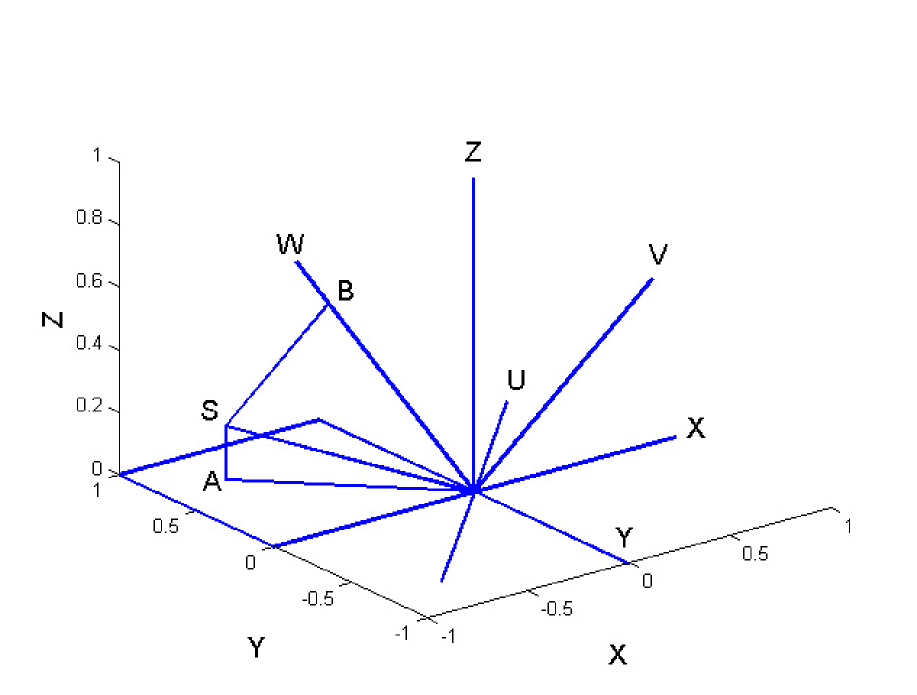
Figure 2: Three dimensional vector space with two sets of incompatible questions

The set of three orthogonal axes labeled $\{\mathbf{X,Y,Z}\}$ represent three different eigenvectors. For example, these three eigenvectors could represent three mutually exclusive and exhaustive responses for a voter such as democrat, republican, or independent (for our purposes, independent means not democrat or republican):

$$\mathbf{X}=\begin{bmatrix}1\\ 0\\ 0\end{bmatrix},\mathbf{Y}=\begin{bmatrix}0\\ 1\\ 0\end{bmatrix},\mathbf{Z}=\begin{bmatrix}0\\ 0\\ 1\end{bmatrix}.$$

The quantum state $\mathbf{\psi}$ is represented in this case by the vector associated with the letter $\mathbf{S}$ in the figure (e.g., the state of an undecided voter just before a presidential election). This state can be described in terms of coordinates with respect to the $\{\mathbf{X,Y,Z\}}$ eigenvectors. In this case, the state assigns the following amplitudes to the $\{\mathbf{X,Y,Z\}}$ eigenvectors

$$\mathbf{\psi}=\mathbf{S}=(-.6963)\cdot\mathbf{X}+(.6963)\cdot\mathbf{Y}+(.1741)\cdot\mathbf{Z}.$$ (2)

Dirac called vectors, such as Equation 2, superposition states with respect to the eigenvectors $\{\mathbf{X,Y,Z\}}$. At this point, a superposition state simply assigns probabilities to events generated by $\{\mathbf{X,Y,Z\}}$, but later this concept takes on a deeper meaning. As can be seen in this example, the amplitudes assigned to each eigenvector can be positive or negative (or even complex numbers). But note that the length of the state vector $\mathbf{S}$ equals one.

Quantum probabilities are expressed most simply and intuitively by using the geometric concept of a projection (see Appendix). In this example, the state vector $\mathbf{S}$ lies in a three dimensional space. The events of interest are subspaces that have smaller dimension (rays or planes in this case). To determine the probability of an event, we first project the state vector on to the subspace that represents the event and then compute its squared length. A matrix is used to perform this projection, which is called the projector for the event. All the quantum events generated by the $\{\mathbf{X,Y,Z}\}$ eigenvectors are based on the following three projectors (formed by outer products):

$$M_{X}=\mathbf{X}\cdot\mathbf{X}^{\dagger},\ M_{Y}=\mathbf{Y}\cdot\mathbf{Y}^{\dagger},\ M_{Z}=\mathbf{Z}\cdot\mathbf{Z}^{\dagger}$$

$$M_{X}+M_{Y}+M_{Z}=I\ (identity).$$

For example, $M_{X}$ is a $3\times 3$ projector matrix (it has a one in the first row and column, and zeros everywhere else), and it projects the state $\mathbf{S}$ on to the ray $X"$ containing the $\mathbf{X}$ eigenvector. The projection equals the matrix product of projector and the state, $M_{X}\cdot\mathbf{S.}$ The probability of event $X"$ (e.g., democrat) equals the square length of the projection $\left|M_{X}\cdot\mathbf{S}\right|^{2}=|-.6963|^{2}=.4848$. The probability of event $Y"$(e.g. republican) is computed in the same way, $\left|M_{Y}\cdot\mathbf{S}\right|^{2}$ $=|.6963|^{2}$ $=.4848$ . Suppose the quantum event in question is the plane formed by the span of eigenvectors $\{\mathbf{X},\mathbf{Y\}}$, which is symbolized as $X"+Y"$ (e.g., ‘democrat or republican’). The projection of the state $\mathbf{S}$ onto the $X"+Y"$ plane is the vector associated with the label $\mathbf{A}$.  The matrix $M_{X+Y}=M_{X}+M_{Y}$ projects the state vector $\mathbf{S}$ onto the subspace $X"+Y"$:

$$\mathbf{A}=M_{X+Y}\cdot\mathbf{S}=\begin{bmatrix}1&0&0\\ 0&1&0\\ 0&0&0\end{bmatrix}\cdot\mathbf{S}=\begin{bmatrix}-.6963\\ .6963\\ 0\end{bmatrix},$$

and the probability of the $X"+Y"$ event equals $|\mathbf{A}|^{2}=$ $|-.6963|^{2}+\left|.6963\right|^{2}=.9697$. The negation of this disjunction event is the ray associated with the $\mathbf{Z}$ eigenvector (e.g., independent), and the probability of this event is $|M_{(X+Y)^{\perp}}\mathbf{\psi}|^{2}=\left|(I-M_{X+Y})\cdot\mathbf{S}\right|^{2}=|M_{Z}\cdot\mathbf{S}|^{2}=|.1741|^{2}=.0303=1-.9697$.

If we were restricted to use only projections on the $\{\mathbf{X,Y,Z}\}$ eigenvectors, then quantum probabilities would obey the same laws as classic probabilities. However, a vector space has no privileged set of eigenvectors. We could rotate the first set $\{\mathbf{X,Y,Z}\}$ of eigenvectors to form a new orthonormal set of eigenvectors labeled $\{\mathbf{U,}$ $\mathbf{V,W}\}$ in the figure. The unitary transformation matrix that generates coordinates for the new eigenvectors $\{\mathbf{U,}$ $\mathbf{V,W}\}$ is

$$T=\begin{bmatrix}1/\sqrt{2}&1/2&-1/2\\ 1/\sqrt{2}&-1/2&1/2\\ 0&1/\sqrt{2}&1/\sqrt{2}\end{bmatrix}=\begin{bmatrix}\mathbf{U}&\mathbf{V}&\mathbf{W}\end{bmatrix}.$$

The first column of $T$ gives the coordinates of the $\mathbf{U}=T\cdot\mathbf{X}$ eigenvector, which is the ray that runs through the main diagonal of the $X"+Y"$ plane. The second and third columns of $T$ give the $\mathbf{V}=T\cdot\mathbf{Y}$ and $\mathbf{W}=T\cdot\mathbf{Z}$ eigenvectors. This new set of eigenvectors $\{\mathbf{U,V,W}\}$ represents a different perspective for understanding features (e.g., moderate, liberal, conservative ). In this (artificial) example, the eigenvector $\mathbf{U}$ (e.g. moderate) lies in the $X"+Y"$ plane and happens to be midway between the eigenvectors $\mathbf{X}$ and $\mathbf{Y}$ (e.g. democrat, republican). All the quantum events generated from the $\{\mathbf{U,V,W}\}$  set of eigenvectors are based on the following three projectors (again formed by outer products):

$$M_{U}=\mathbf{U}\cdot\mathbf{U}^{\dagger},\ M_{V}=\mathbf{V}\cdot\mathbf{V}^{\dagger},\ M_{W}=\mathbf{W}\cdot\mathbf{W}^{\dagger}$$

$$M_{U}+M_{V}+M_{W}=I.$$

The state vector $\mathbf{\psi}=\mathbf{S}$ can also be described in terms of the amplitudes assigned to the new eigenvectors $\{\mathbf{U,V,W}\}.$ The matrix product

$$T^{\dagger}\cdot\mathbf{S=}\begin{bmatrix}\mathbf{U}^{\dagger}\\ \mathbf{V}^{\dagger}\\ \mathbf{W}^{\dagger}\end{bmatrix}\cdot\mathbf{S=}\begin{bmatrix}\mathbf{U}^{\dagger}\cdot\mathbf{S}\\ \mathbf{V}^{\dagger}\cdot\mathbf{S}\\ \mathbf{W}^{\dagger}\cdot\mathbf{S}\end{bmatrix}=\begin{bmatrix}0\\ -.5732\\ .8194\end{bmatrix}.$$

transforms the amplitudes originally assigned to eigenvectors $\{\mathbf{X},\mathbf{Y},\mathbf{Z}\}$ into amplitudes assigned to eigenvectors $\{\mathbf{U},\mathbf{V},\mathbf{W}\}$. This allows us to express the state $\mathbf{S}$ as a superposition state with respect to the eigenvectors $\{\mathbf{U,V,W\}}$. In other words, the exact same state $\mathbf{S}$ can be expressed as a superposition of the $\{\mathbf{X,Y,Z\}}$ eigenvectors or as a superposition of the $\{\mathbf{U,V,W\}}$ eigenvectors:

$$(-.6963)\cdot\mathbf{X}+(.6963)\cdot\mathbf{Y}+(.1741)\cdot\mathbf{Z=S}$$ (3)

$$=I\cdot\mathbf{S}=(M_{U}+M_{V}+M_{W})\cdot\mathbf{S}$$

$$=\mathbf{U}\cdot\mathbf{U}^{\dagger}\cdot\mathbf{S}+\mathbf{V}\cdot\mathbf{V}^{\dagger}\cdot\mathbf{S}+\mathbf{W}\cdot\mathbf{W}^{\dagger}\cdot\mathbf{S}$$

$$=0\cdot\mathbf{U}+(-.5732)\cdot\mathbf{V}+(.8194)\cdot\mathbf{W.}$$

Now the concept of superposition becomes much deeper because the same state $\mathbf{S}$ must generate probabilities for two different sets of eigenvectors. Shortly we will show how superposition states with respect to different sets of eigenvectors produce interference effects that are critical for explaining violations of classic probability theory. But first, let us continue with a few more example calculations. The probability of the event $W"$ (e.g. conservative) is determined by projecting the state $\mathbf{S}$ on to the eigenvector $\mathbf{W}$, using the projector $M_{W}$, which produces the projection associated with the vector labeled $\mathbf{B}$ in the figure. The squared length of this projection equals

$$q(W") =|\mathbf{B}|^{2}=|M_{W}\cdot\mathbf{S}|^{2}$$

$$=|\mathbf{W}\cdot\mathbf{W}^{\dagger}\cdot\mathbf{S}|^{2}$$

$$=|\mathbf{W}|^{2}\cdot|\mathbf{W}^{\dagger}\cdot\mathbf{S}|^{2}=1\cdot|\mathbf{W}^{\dagger}\cdot\mathbf{S}|^{2}$$

$$=|.8194|^{2}=.6714,$$

which is simply the squared magnitude of the amplitude assigned to $\mathbf{W}$ in Equation 3.

Finally consider the conditional probability of event $W"$ given that event $X"+Y"$ has occurred (e.g., the probability that the voter is conservative given that the person voted for a democrat or republican). Following Lüder’s rule, we first compute the normalized projection of the original state $\mathbf{S}$ on the known event $X"+Y"$. Recall from above that $\mathbf{A}$ is the projection, and this is normalized to form the vector $\mathbf{\psi}_{X+Y}=\mathbf{A}/\left|\mathbf{A}\right|=\begin{bmatrix}-1/\sqrt{2}&1/\sqrt{2}&0\end{bmatrix}^{\dagger}.$ Then we compute the squared length of the projection of the state $\mathbf{\psi}_{X+Y}$ onto the ray $W"$, which equals $q(W"|X"+Y")=\left|M_{W}\cdot\mathbf{\psi}_{X+Y}\right|^{2}$ $=|(W\cdot W^{\dagger}\cdot\mathbf{A}/|\mathbf{A}|)|^{2}=.50$.  Similarly, the probability $q(W"|Z")=$ $\left|M_{W}\cdot\mathbf{Z}\right|^{2}=.50.$

A cognitive processing interpretation of the basic quantum principles can now be given by using the geometric concepts of states and projectors. The eigenvectors correspond to feature patterns that are used to describe or characterize events. The initial state vector $\mathbf{\psi}$ represents the memory trace that determines the potential for a pattern to be retrieved, which is formed by the person’s prior knowledge and the story told to the person. When questioned about a single event $A$, a projector $M_{A}=\sum\mathbf{V}_{j}\cdot\mathbf{V}_{j}^{\dagger}$ is formed from the features (eigenvectors) $\{\mathbf{V}_{j}$, $j\in A"\}$ representing the question $A$. The projection, $M_{A}\cdot\mathbf{\psi}$, determines how well the retrieval cue provided by the question matches the memory state, and the probability of a retrieval equals the squared length of the projection: $q(A")=\left|M_{A}\cdot\mathbf{\psi}\right|^{2}=\sum_{V_{j}\in A"}\left|\psi_{j}\right|^{2}$. If event $A"$ is assumed to be true, then the initial state $\mathbf{\psi}$ changes to a new state $\mathbf{\psi}_{A}$, which is the normalized projection $\mathbf{\psi}_{A}=$ $(M_{A}\cdot\mathbf{\psi})/\left|M_{A}\cdot\mathbf{\psi}\right|.$ After given this information, if a second question is asked about event $B$, then a projector $M_{B}=\sum\mathbf{W}_{j}\cdot\mathbf{W}_{j}^{\dagger}$ is formed from the features (eigenvectors) $\{\mathbf{W}_{j}$, $j\in B"\}$ representing the question $B$, and the conditional probability of a positive response to the retrieval cue $B"$ after given information about $A"$ equals $q(B"|A")=\left|M_{B}\cdot\mathbf{\psi}_{A}\right|^{2}$. Finally, the probability of a positive response to the conjunction equals the probability of positive retrievals to both the first and second questions

$$q(A"\sqcap B") =q(A")\cdot q(B"|A")$$ (4)

$$=\left|M_{A}\cdot\mathbf{\psi}\right|^{2}\cdot\left|M_{B}\cdot\mathbf{\psi}_{A}\right|^{2}$$

$$=\left|M_{A}\cdot\mathbf{\psi}\right|^{2}\cdot\left|M_{B}\cdot\frac{(M_{A}\cdot\mathbf{\psi})}{\left|M_{A}\cdot\mathbf{\psi}\right|}\right|^{2}$$ (5)

$$=\left|M_{B}\cdot M_{A}\cdot\mathbf{\psi}\right|^{2}.$$

3.2 Interference

The possibility of using different sets of eigenvectors, $\{\mathbf{X,Y,Z}\}$ versus $\{\mathbf{U}$ ,$\mathbf{V}$,$\mathbf{W}\}$, within the same vector space to represent different types of questions introduces an important psychological issue about the disturbance or interference of one question by another. Suppose we ask about a question about event $W$ (e.g. conservative). Before we ask this question, while the person is in the initial state $\mathbf{S}$, there is a .6714 probability of answering yes. After obtaining this answer, the state changes (according to Lüder’s rule) from state $\mathbf{S}$ to state $\mathbf{W}$. If we ask the same question again immediately, the person will answer yes with certainty (and with frustration for being asked to repeat the answer). The state $\mathbf{W}$ is no longer in superposition with respect to the $\{\mathbf{U,V,W\}}$ eigenvectors. However, this same state $\mathbf{W}$ is in superposition with respect to the $\{\mathbf{X,Y,Z\}}$ eigenvectors. In other words, once a person becomes certain about the $\{\mathbf{U,V,W\}}$ set of eigenvectors, this person must become uncertain with respect to the $\{\mathbf{X,Y,Z\}}$ set of eigenvectors. The person can’t be certain about both at the same time (Heisenberg called this the uncertainty principle). Furthermore, if we now ask a question about event $Y$ (e.g., republican), then the probability of a yes equals .25 (given state $\mathbf{W}$). If the answer to the $Y$ question happens to be yes, then the state changes (according to Lüder’s rule again) from $\mathbf{W}$ to $\mathbf{Y},$ and the person becomes certain about the $Y$ question, but becomes uncertain again about the $W$ question (probability of yes to question $W$ given state $\mathbf{Y}$ is also .25). In other words, asking the question about $Y$ after the answer to question $W$ has changed the likelihood of responses about question $W$ from certainty to uncertainty again. (This is the reason filler items are inserted in between repetitions of a question). This type of disturbance between questions can always happen with superposition states described by different sets of eigenvectors within the same vector space.

3.3 Compatibility of events

According to quantum theory, order is usually critical, and one has to be careful of the order that questions are asked. For example, a projection on $X"$ followed by a projection on $U"$is not the same as these operations in reverse ($M_{X}\cdot M_{U}\neq M_{U}\cdot M_{X}$, i.e., the projection matrices do not commute). In other words, asking question $X$ first (e.g. whether a person is a democrat or not) followed by asking question $U$ (e.g., whether a person is a moderate or not) is not necessarily the same as asking these questions in the opposite order. This order effect indicates the property of incompatibility between these two events (they do not share the same eigenvectors). Psychologically, one can only view one perspective at a time, the questions must be answered sequentially, and as we have seen, asking one question from one perspective can disturb a later question from a different perspective (for example, first asking about being a moderate can disturb a later question about being a democrat). There is an abundance of research demonstrating order effects on probability judgments [47]. For example, when judging probabilities of guilt in a criminal trial, the direction of the effect of weak evidence on judgments depends on whether it precedes or follows strong evidence [48]. These order effects are inconsistent with classic probability theory, and in the past, they have been explained in terms of anchoring and adjustment type of adding or averaging models.

This capability of changing eigenvectors (i.e. changing perspectives) and producing incompatible events makes quantum theory fundamentally different than classic theory. Classic (Kolmogorov) probability theory assumes a single compatible representation of events. Figure 2 was constructed assuming that quantum events $X",Y",Z"$ (e.g., democrat, republican, independent) are incompatible with the quantum events $U",V",W"$(e.g., moderate, liberal, conservative). In this case, one set of events is a rotation of the other set of events within the same three dimensional space as depicted in Figure 2. To evaluate a question about the $X$ event, we need to adopt the $\{\mathbf{X,Y,Z}\}$ eigenvector point of view; but then to evaluate a question about the $U$ event, we need to rotate to the $\{\mathbf{U,V,W}\}$ eigenvector perspective. One cannot evaluate questions about $X$ and $U$ simultaneously (Bohr called this the principle of complementarity).

Alternatively, note that whenever we ask questions using eigenvectors from the same set, then the order does not matter. For example, $M_{X}\cdot M_{Y}=M_{Y}\cdot M_{X}$ so $X"$ (e.g. is a person a democrat) is compatible with $Y"$ (e.g., is a person a republican). This lack of order effect defines the property of compatibility between these two events (they share the same eigenvectors). In this case one can maintain the same perspective while answering both questions. In this way, the questions can be answered simultaneously, because one question does not disturb the other. In this case the two events $X",Y"$ are also mutually exclusive (i.e., orthogonal subspaces), and so are the two events $U",V"$. In general, if two events $M_{A},M_{B}$ are orthogonal to each other, then they are compatible because $M_{A}\cdot M_{B}=0=M_{B}\cdot M_{A}.$ However, it is possible that two events can be compatible yet not orthogonal. For example, $M_{U+V}\cdot M_{V+W}=M_{V}=M_{V+W}\cdot M_{U+V}$  and so $U"+V"$ (e.g., is a person a moderate or liberal) is compatible with $V"+W"$ (e.g., a person is liberal or conservative).

Now let us turn and examine the geometric situation used to represent events when they are all compatible. Once again suppose that $\{X",Y",Z"\}$ represent three mutually exclusive and exhaustive quantum events (e.g., a person is a democrat, republican, independent); and suppose that $\{Q",R",S"\}$ is a different set of three mutually exclusive and exhaustive quantum events (e.g., a person is young, middle age, or old). As before, the events in $\{X",Y",Z"\}$ are not necessarily orthogonal to the events in $\{Q",R",S"\}$,  but now we assume that the events in $\{X",Y",Z"\}$ are compatible with the events in $\{Q",R",S"\}.$ This implies not only that $M_{X}\cdot M_{Y}=M_{Y}\cdot M_{X}$ but also that $M_{X}\cdot M_{Q}=M_{Q}\cdot M_{X}$, and this is true for all pairs of events. Now it is impossible to represent all these events by Figure 2, because all of these compatible properties cannot occur within a 3 dimensional space. These compatible events require (at least) a 9-dimensional vector space (see Appendix) based on 9 orthonormal eigenvectors $\{\mathbf{XQ},\mathbf{XR},\mathbf{XS}$,$\mathbf{YQ},\mathbf{YR},\mathbf{YS}$,$\mathbf{ZQ},\mathbf{ZR},\mathbf{ZS}\}$, which is forms a tensor product space. In this 9-dimensional vector space, the single ray or eigenvector $\mathbf{XQ}$ represents the pattern or joint event $X"\cap Q"$ (e.g. democrat and young), and the amplitude assigned to the $\mathbf{XQ}$ eigenvector determines the joint probability of $X"\cap Q"$. Using this representation, the event $X"=XQ"+XR"+XS"$ (e.g., democrat) corresponds to the projector $M_{X}=(M_{XQ}+M_{XR}+M_{XS})$, the event $Q"=XQ"+YQ"+ZQ"$ (e.g., young) corresponds to the projector $M_{Q}=(M_{XQ}+M_{YQ}+M_{ZQ})$, the intersection event $(X"\cap Q")=XQ"$ corresponds to the projector $M_{X\cap Q}=M_{X}\cdot M_{Q}=$ $M_{Q}\cdot M_{X}=M_{XQ}$ $=\mathbf{XQ}\cdot\mathbf{XQ}^{\dagger},$ and the span $X"+Q"$ corresponds to $M_{X+Q}=M_{X}+M_{Q}-M_{Q}\cdot M_{X}$. If all of the events are compatible, then the probabilities computed from quantum theory obey the same laws as the probabilities computed from classic (Kolmogorov) theory (see Appendix).

In summary, if events $\{X",Y",Z"\}$ and events $\{U",V",W"\}$ are incompatible, then the person can only respond with one of three possible outcomes at any point in time. The person can choose a response from the set $\{X",Y",Z"\},$ or the person can choose a response from the set $\{U",V",W"\},$ but we cannot observe any combinations. So this situation can be represented within a 3-dimensional space. But when the events in $\{X",Y",Z"\}$ and $\{Q",R",S"\}$ are compatible, then a person can respond with a pair, one from each set, which means one of 9 possible outcomes can occur. So we need to use at least a 9 - dimensional space to represent this situation. These are the smallest possible dimensions that could be used for these examples, and in general, the dimensionality could be much larger in both cases.

Of course it is possible to have a combination of compatible and incompatible events. For example, suppose we had three sets of questions: a first set of mutually exclusive and exhaustive events $\{X",Y",Z"\}$, a second set of mutually exclusive and exhaustive events $\{U",V",W"\}$, and a third set of mutually exclusive and exhaustive events $\{Q",R",S"\}$. Again we suppose that a question taken from one set is not orthogonal to a question taken from a different set. In this situation it is possible, for example, to have the first and second set be incompatible with each other, but both could be compatible with the third set. This situation would require at least a 9-dimensional space. This vector space would be spanned by 9 eigenvectors formed from combinations of the first and third sets, or it would be spanned by 9 eigenvectors formed from combinations of the second and third sets; furthermore the two sets of eigenvectors would be related by a unitary transformation.

When should events be treated as compatible or incompatible? The general answer is that this is an empirical question, and order effects are an empirical sign of incompatibility. However, at this point we make the working hypothesis that compatibility depends on experience with the combination of events. Conjunction errors disappear when individuals are given direct training experience with pairs of events [49], and order effects on abductive inference also decrease with training experience [50]. On the one hand, if the person has a great deal of experience with the combination or pattern of events, then they have the opportunity to form a compatible vector space, and they can estimate the intersection of events from this large space of patterns of events. On the other hand, if an unusual or novel combination of events is presented, and the person has little or no experience with such combinations, then they may not have formed a compatible representation, and they must rely on incompatible representations of events that use the same small vector space but require taking different perspectives. A second way to facilitate the formation of a compatible representation is to present the required joint frequency information in a tabular format [51]. Instructions to use a joint frequency table format would encourage a person to form and make use of a compatible representation that assigns amplitudes to the cells of the joint frequency tables.

3.4 Violations of commutative and distributive properties

Quantum probabilities for sequential conjunctions violate the commutative property. For example, referring to Figure 2, consider the quantum probability for conjunctive questions about events $X$ (e.g., democrat) and $U$ (e.g., moderate) again. The probability of agreeing to both when question $X$ is queried first and question $U$ is asked second equals $q(X"\sqcap U")=\left|M_{U}M_{X}\cdot\mathbf{S}\right|^{2}=.2424,$ and the probability of yes to both in the opposite order is $q(U"\sqcap X")=\left|M_{X}M_{U}\cdot\mathbf{S}\right|^{2}=0.$ This dramatic change in order happens in this case for the following reason. The initial state $\mathbf{S}$ for the individual shown in the figure is orthogonal to the vector $\mathbf{U}$. If this individual is initially asked about question $U$ (e.g., are you a moderate?), then there is zero probability of answering yes to this first question (e.g., a person who likes to take a strong stand on issues), and so the conjunctive probability is also zero. However, if the individual is initially asked about the question $X$, then the initial state $\mathbf{S}$ is negatively correlated to the vector $\mathbf{X}$ (e.g. democrat), and its squared magnitude makes a reasonable probability of saying yes and transiting from the $\mathbf{S}$ to the $\mathbf{X}$ state; furthermore the $\mathbf{X}$ state (e.g. democrat) is positively correlated to the $\mathbf{U}$ state (e.g., moderate), which then makes it possible to transfer from $\mathbf{X}$ to $\mathbf{U}$ and answer yes to the second question as well. In fact, it is well known that survey responses can be manipulated by order [52], and similar ‘chaining’ effects are found in categorization [53]. Quantum probabilities for disjunctions also violate the commutative property. For example, consider once again Figure 2. The quantum probability for the disjunction question $(X\vee U)$ assuming that question $X$ is processed first equals $q(X"\sqcup U")=$ $1-\left|M_{U^{\perp}}M_{X^{\perp}}\cdot S\right|^{2}=.7273,$ and for the other order it is $q(U"\sqcup X")=$ $1-\left|M_{X^{\perp}}M_{U^{\perp}}\cdot S\right|^{2}=.4848.$ These differ because $q(U")=0$ for the latter order.

There is considerable direct evidence for order effects on the conjunctive fallacy.  In the first experiment of Gavansky and Roskos-Ewoldsen (1991), participants rated the individual constituents before rating the conjunction (producing the circles in Figure 1), and in the second experiment the conjunction was rated first (producing the dots in Figure 1). As can be seen, rating the conjunction first produced a larger magnitude conjunction error. These results were replicated using random assignment to two groups within a single study by Stolarz-Fantino et al. (2003, Exp 2). When the conjunction came first, the mean probability rating for the conjunction equaled .26 as compared to a mean of .18 for the low event, and 57% of the participants produced the error; but for the opposite order the mean rating for the conjunction was .16 as compared to a mean of .14 for the low likelihood event, and only 31% of the participants produced the error.

The law of total probability is fundamental to Bayesian theory, but according to quantum theory, it fails when incompatible events ever are involved. To see how and why this happens, we return to Figure 2. Consider the probability for a question about event $W$ (e.g., whether or not a person is a conservative). According to classic probability theory, a positive response to this question can happen two mutually exclusive and exhaustive ways: the person is an independent and a conservative $(Z^{\prime}\cap W^{\prime})$, or the person is not an independent and a conservative $(\overline{Z}\cap W^{\prime})$. So the total probability that a person is a conservative equals $\mathbf{p}(W^{\prime})=\mathbf{p}((Z^{\prime}\cup\overline{Z})\cap W)=\mathbf{p}(Z^{\prime})\cdot\mathbf{p}(W^{\prime}|Z^{\prime})+\mathbf{p}(\overline{Z})\cdot\mathbf{p}(W^{\prime}|\overline{Z}).$ Now let us reconsider the quantum probabilities that we computed earlier for these events using Figure 2. When we first asked a question about $Z$ and then asked about $W$, recall that we found $q(Z")=.0303$ and $q(W"|Z^{\perp})=q(W|Z")=.50,$ and so the total probability is $q((Z"\sqcap W")\sqcup(Z^{\perp}\sqcap W"))=$ $q(Z")\cdot q(W"|Z")+q(Z^{\perp})q(W"|Z^{\perp})=.50$. But if we directly ask a person a question about event $W$, then we found earlier that $q(W")=q((Z"\sqcup Z^{\perp})\sqcap W")=.6714$, which violates the law of total probability! The reason that this happened is because the initial state $\mathbf{S}$ is very similar to the ray $W"$, but the initial state $\mathbf{S}$ is very dissimilar to the ray $Z"$ which must be reached first by one of the two indirect routes from $\mathbf{S}$ passing through $Z"$ or $Z^{\perp\text{ }}$to $W".$ Violations of the law of total probability have in fact been reported in some of earlier research [54]. This violation of the law of total probability by quantum theory will turn out to be one of the key ideas to explain the fallacies reviewed earlier. This only happens when events are incompatible.

What determines the order for incompatible questions? This is an important empirical issue. A working hypothesis is that when the individual events differ greatly in terms of their likelihoods (e.g. for the Linda story, the event feminist is very likely whereas the event bank teller is very unlikely), then people start with the higher probability event. For the conjunction question $(H\wedge L)$ this implies using the $(H"\sqcap L")$ conjunctive sequence. For example, when asked the conjunction question regarding the Linda story, we assume that the feminist event is processed before the bank teller event. But for the disjunction question $(H\vee L)$, the relevant conjunction question that needs to be considered is $(\char 126\relax H\wedge\char 126\relax L)$, and $\char 126\relax L$ is more likely than $\char 126\relax H$. So the ‘start with the higher probability’ principle implies using the conjunctive sequence $(L^{\perp}\sqcap H^{\perp}),$ which implies using the disjunctive sequence $(L"\sqcup H")$. For example, when asked the disjunction question regarding the Linda story, we assume that the not-bank teller event is processed before the not-feminist event. Another factor that determines order of processing is a cause - effect relation, i.e., if $C$ is the cause and $E$ is the effect, then we assume $(C"\sqcap E")$. For example, when given the ‘increase tax and reduce smoking problem’, we assume that the ’tax’ cause is processed first.

4 Quantum Explanation of Judgment ‘Errors’

The quantum model is essentially a similarity based approach to probability, where similarity is determined by inner products of vectors in a multidimensional space. Thus it is quite consistent with the finding that typicality rating conjunction effects are highly correlated with conjunction errors (Fact 14).  In fact, it has already proved to be highly successful for modeling typicality ratings for conjunctive and disjunctive concepts [6]. But how do conjunction and disjunction errors arise in the first place? We now turn to these more challenging questions.

4.1 Conjunction error and its moderators

Let us first consider a single conjunction fallacy (Fact 1). The state vector $\mathbf{\psi}$ represents the memory state of the individual after reading the story (which is based on both prior knowledge together with details about the story). The projector, $M_{H}$ serves as a retrieval cue for retrieving features related to the question about event $H$ (feminist); and similarly, the projector $M_{L}$ serves as the retrieval cue for questions about event $L$ (bank teller). Thus $M_{H}$ projects the Linda state $\mathbf{\psi}$ onto the high likelihood image of feminist, and $M_{L}$ projects the Linda state $\mathbf{\psi}$ onto the low likelihood image of bank teller. According to the ‘start with the higher probability’ rule, the probability for the sequential conjunction is $q(H"\sqcap L")=\left|M_{L}\cdot M_{H}\cdot\mathbf{\psi}\right|^{2}$, and the probability for the single event is $q(L")=\left|M_{L}\mathbf{\psi}\right|^{2}$. So how can we (the theorists) tell whether or not the fallacy occurs? To do this, we (the theorists, not the judge) need to express the single event probability in terms of the conjunction probabilities using the quantum rules (see Appendix for details):

$$q(L") =\left|M_{L}\mathbf{\psi}\right|^{2}=\left|M_{L}\cdot I\cdot\mathbf{\psi}\right|^{2}$$ (6)

$$=\left|M_{L}\cdot(M_{H}+M_{H^{\perp}})\cdot\mathbf{\psi}\right|^{2}$$

$$=q(H"\sqcap L")+q(H^{\perp}\sqcap L")+Int_{L}$$

$$Int_{L}=2\cdot\operatorname{Re}[(M_{L}M_{H^{\perp}}\mathbf{\psi})^{\dagger}(M_{L}M_{H}\mathbf{\psi})].$$ (7)

Notice that the quantum probability (Equation 6) almost looks like the law of total probability (Equation 1), except for the interference term, $Int_{L}$ (associated with event $L")$, which can be positive, negative, or zero. This interference is the same mathematical concept that is used to explain the classic two hole experiment with photons in physics [55]. If the interference term is zero, then quantum probabilities satisfy the law of total probability and no conjunction error occurs. Thus the model allows some people to be consistent with classic probability theory. In particular, if $M_{H}$ and $M_{L}$ are compatible, then this interference term is exactly zero (see Appendix). Thus interference only occurs with incompatible events, and this explains why conjunction errors are robust for questions about unrelated events $H_{1}$ and $L_{2}$ concerning different people (Fact 13b). For this is exactly a situation in which it is unlikely that a person has sufficient experience to form a compatible representation, and must represent the situation with incompatible events that interfere.

To produce the conjunction ‘error’ we require $Int_{L}<-q(H^{\perp}\sqcap L")<0,$ and because $q(H^{\perp}\sqcap L")\geq 0,$ this implies that the interference must be sufficiently negative to produce a conjunction error. This last result explains the fact the conjunction errors occur more frequently with questions about mixed $H$ and $L$ events (Fact 12): $q(H^{\perp}\sqcap L")$ must be small to produce the conjunction fallacy. Note that if $H$ is a question about a high likelihood event, then $H^{\perp}$ is a low likelihood quantum event, and $L"$ is also a low likelihood quantum event, which makes $q(H^{\perp}\sqcap L")$ small, and so only a small negative amount of interference is needed. This does not happen for the low -low case (because $q(L_{1}^{\perp}\sqcap L_{2}")$ has one high component), or the high -high case (because $q(H_{1}^{\perp}\sqcap H_{2}")$ has one high component), and so the interference may be insufficient to produce the conjunction error in these cases. In fact, the size of the conjunction error is bounded by the difference between $q(H")\geq q(H"\sqcap L")\geq$ $q(L")$, and it shrinks to zero if $q(H")=q(L")$ (see Appendix). This in fact matches the results shown in Figure 1. There it can be seen that the conjunction error is present only for mixed $H$ and $L$ events on the left wall, and it is absent for events on the diagonal of the X-Y plane, where $q(A)$ is almost equal to $q(B)$. Furthermore, consistent with Fact 12, only single conjunction errors are predicted to occur in the high-low case, because the interference effect is only produced for the $L"$ quantum event when sequentially processed in the $(H"\sqcap L")$ order (see a later section for the double conjunction error issue).

How do we psychologically interpret this interference effect? Consider, for example, Figure 2 once again. Suppose we compare the conjunction probabilities $q(X"\sqcap U")$ and $q(X^{\perp}\sqcap U")$ with the probability of the single event $q(U")$ given state $\mathbf{S}$ in the figure. These calculations produce the following answers: $q(X"\sqcap U")$ $=\left|M_{U}M_{X}\cdot\mathbf{S}\right|^{2}$ $=.2424$ and $q(X^{\perp}\sqcap U")$ $=\left|M_{U}(M_{Y}+M_{Z})\cdot\mathbf{S}\right|^{2}$ $=.2424$ but $q(U")$ $=\left|M_{U}\cdot\mathbf{S}\right|^{2}=0$ and so $Int_{U}=-.4848$. The first term, $q(X"\sqcap U"),$ is positive because $\mathbf{S}$ is negatively correlated with $\mathbf{X}$, and $\mathbf{X}\,$ is positively correlated with $\mathbf{U}$ in the figure, and so the squared magnitude is positive. The second term is positive for the same kind of reasoning.  But $\mathbf{S}$ is orthogonal to $\mathbf{U}$ in the figure. The psychological intuition behind this math is the following – while it is possible to reach the conclusion $\mathbf{U}$ by way of thinking first about $\mathbf{X}$ from state $\mathbf{S,}$ it is impossible to reach this conclusion directly from state $\mathbf{S}$. In other words, the indirect line of thought $\mathbf{S}\rightarrow\mathbf{X}\rightarrow\mathbf{U}$ has a reasonable possibility even though there is no chance from the direct route $\mathbf{S}\rightarrow\mathbf{U}$. You cannot see the conclusion $\mathbf{U}$ directly from state $\mathbf{S}$; but the indirect route (produced by asking about question $X$ first) puts you in a state that makes you think of something different, which then opens the possibility of reaching a conclusion favoring yes to question $U$. For the Linda story, the judge cannot directly imagine Linda as a bank teller; but if the judge first thinks about her as a feminist, and then imagines her as a bank teller from this new feminist point of view, it now seems more possible that she could be a bank teller. This quantum explanation relates to both the availability and representativeness heuristics. The representativeness heuristic comes into play when matching the story to each question in terms of similarity, and the availability heuristic comes into play when one question acts as a retrieval cue redirecting thinking toward a different point of view.

The interference term can also be expressed as $Int_{L}=q(L")-[q(H"\sqcap L")+q(H^{\perp}\sqcap L")].$ The first term, $q(L"),$ is the probability of reaching a conclusion from a direct route (initial state to conclusion). The bracketed term is the probability of reaching the same conclusion summed across all indirect routes (through an incompatible set of eigenstates) to that conclusion. Thus $Int_{L}$ is a quantity that we (the theorist) derive to express the difference in probabilities caused by traveling the direct route versus traveling a set of indirect routes, and different interference terms can be derived depending on which set of indirect routes we compare to the direct route. When the interference term is negative, that means that the indirect routes have a greater chance of reaching the conclusion; and when the interference term is positive, that means that the direct route has a greater chance of reaching the conclusion. The interference term can be directly estimated from experiments that request all three judgments $J(A)$, $J(A\wedge B)$, $J(A\wedge\char 126\relax B)$. This procedure was carried out in the study by Wedell and Moro (2008), and using the data reported in Table 2 from that article, we obtain the following interference estimates: $-.36$ for the dice problem, and $-.55$ for the urn problem. The calculation of the interference effect, $-.4848$, based on Figure 2 is an example of a conjunction ‘fallacy’ produced simply by using the inner products (similarities) between vectors in the figure, and more exact results can be obtained by adjusting these inner products. The inner products between vectors are the key parameters for making exact predictions, and the model could be fit to judgments using some type of multidimensional scaling algorithm. (This would also require a more sophisticated response model.)

Note that $\operatorname{Re}[(M_{L}M_{H^{\perp}}\mathbf{\psi})^{\dagger}\cdot(M_{L}M_{H}\mathbf{\psi})]$ is the real part of the inner product between two vectors, $M_{L}M_{H^{\perp}}\mathbf{\psi}$ and $M_{L}M_{H}\mathbf{\psi}$. The first vector, $M_{L}M_{H^{\perp}}\mathbf{\psi}$ is the projection of the state $\mathbf{\psi}$ (produced by the story) first on the $H^{\perp}$ subspace and then on to the $L"$ subspace; the second vector is the projection of the same state $\mathbf{\psi}$ (created by the story) now on the $H"$ subspace and then again on the $L"$ subspace. For the Linda story, $M_{B}M_{F^{\perp}}\mathbf{\psi}$ captures the features that match the Linda story with a type of person who is first considered not to be a feminist and then considered also to be a bank teller; $M_{B}M_{F}\mathbf{\psi}$ captures the features that match the Linda story with a type of person who is first considered to be a feminist and then again considered also to be a bank teller. Recall that an inner product is like a correlation: If these two vectors match or are similar, then the inner product will be positive; but if these two vectors mismatch or are dissimilar, then the inner product will be negative; and if the two vectors are unrelated or orthogonal, then the inner product will be zero. Although not many features match between the Linda story and a person who is not feminist and a bank teller; those that do match are likely to have some negative relation to those that match a person who is a feminist and a bank teller, resulting in a negative inner product and producing negative interference. More generally, the relation between the features of the quantum events $H"$ and $L"$, as well as their match to the story, are important for determining the size and direction of interference. This is important for explaining Facts 10,11. The interference depends on the inner product of projections on event subspaces, and this inner product provides a principled way to understand the effects of semantics and interdependence of events on conjunction errors. This inner product also allows for effects of relationship between events that are sometimes found (but not necessary) for conjunction errors (Fact 13a).

A similar analysis applies to the studies of the conjunction fallacy that employ cause – effect type of events. For example, suppose the two quantum events are $C"$ (e.g., ‘increase cigarette tax’) and $E"$ (e.g. ‘reduce smoking’).  The ‘cause first’ order principle specifies that the prediction for the conjunction is $q(C"\sqcap E"),$ and the prediction for the single event $E"$ is

$$q(E") =\left|M_{E}\mathbf{\psi}\right|^{2}=\left|M_{E}\cdot I\cdot\mathbf{\psi}\right|^{2}=\left|M_{E}\cdot(M_{C}+M_{C^{\perp}})\cdot\mathbf{\psi}\right|^{2}$$ (8)

$$=q(C"\sqcap E")+q(C^{\perp}\sqcap E")+Int_{E}.$$

With negative interference produced by the sequential conjunctive judgment, $Int_{E}<-$ $q(C^{\perp}\sqcap E")$, the quantum probabilities again produce a conjunction fallacy $q(C"\sqcap E")>q(E")$. Again the psychological intuition is the following. From the initial state, it is hard to imagine why teenage smoking should decrease; but it is not hard to imagine a tax increase on cigarettes, and once you imagine that, it is not hard to imagine a drop in teenage smoking. If there is a strong causal relation, then $q(C"\sqcap E")$ $=q(C")\cdot q(E"|C")$ is large (because $q(E"|C")$ is large) and $q(C^{\perp}\sqcap E")=q(C^{\perp})\cdot q(E"|C^{\perp})$ is small (because $q(E"|C^{\perp})$ is small), and the conjunction fallacy is more likely to occur. A positive conditional dependency between the cause and effect increases the joint probability $q(C"\sqcap E")$ and decreases the joint probability $q(C^{\perp}\sqcap E")$, which agrees with Fact 11. The interference in this case equals $Int_{E}=\operatorname{Re}[(M_{E}M_{C^{\perp}}\mathbf{\psi})^{\dagger}\cdot(M_{E}M_{C}\mathbf{\psi})]$. This means that the inner product must be negative between (a) the projection first on the cause absent followed by the effect, and (b) the projection first on the cause present followed by the effect. In other words, the features produced by situations associated with the cause absent and effect present are negatively correlated with the features associated with the cause present and the effect present.

It is time to address the issue of double conjunction errors. Double conjunction errors occur more frequently for conjunctions that contain two highly likely constituents. However, as can be seen in Figure 1, double conjunction errors are not found using means even for $H\wedge H$ events. Quantum theory can only produce zero or single conjunction errors. If $q(A")>q(B")$, then a single conjunction error, $q(A"\sqcap B")>q(B")$, is possible (see Appendix). Double conjunction errors obtained from a single rank ordering of a list of events can be interpreted in one of two ways. First, they may simply be the result of judgment error. This is a likely explanation for two reasons. One is that they do not occur with the means after averaging out the error. Second, chance errors from a single rank ordering of a list of events are very likely when the event probabilities are nearly equal. In particular, if one assumes that people correctly use the multiplicative rules of classic probability theory, but base these calculations on noisy probability estimates, then more frequent conjunction errors are predicted to occur by chance for the $H\wedge H$ case [43]. A second, and possibly more interesting reason, is that double conjunction errors may reflect an unusual situation in which the formation of an entirely new unitized or configural concept emerges. More formally, a new subspace $AB"$ is formed that corresponds to a projector which cannot be decomposed into a product of the two projectors for the subspaces, $A",B"$. The quantum concept of entanglement has been used to describe this new type of configuration [6].

4.2 Disjunction errors and unpacking effects

Next let us consider the disjunction fallacy (Fact 2). Once again $\mathbf{\psi}$ is the memory state following the Linda story, $M_{H}$ is the retrieval cue or projector for feminist, and $M_{L}$ is the retrieval cue or projector for bank teller. The quantum probability of the single event is $q(H")=1-q(H^{\perp})$ and the quantum probability for the disjunction is $q(L"\sqcup H")=1-q(L^{\perp}\sqcap H^{\perp}).$ Therefore, the disjunction fallacy requires $q(H")>q(L"\sqcup H")$ $\ \mapsto q(H^{\perp})<q(L^{\perp}\sqcap H^{\perp}).$ We (the theorists) can compare these predictions by expanding $q(H^{\perp})$ like we did for $q(L")$ in Equation 6:

$$q(H^{\perp}) =\left|M_{H^{\perp}}\cdot\mathbf{\psi}\right|^{2}=\left|M_{H^{\perp}}\cdot(M_{L}+M_{L^{\perp}})\cdot\mathbf{\psi}\right|^{2}$$ (9)

$$=q(L"\sqcap H^{\perp})+q(L^{\perp}\sqcap H^{\perp})+Int_{H^{\perp}},$$

$$Int_{H^{\perp}} =\operatorname{Re}[(M_{H^{\perp}}M_{L}\mathbf{\psi})^{\dagger}\cdot(M_{H^{\perp}}M_{L^{\perp}}\mathbf{\psi})].$$

Using this result, we find that we require negative interference again, $Int_{H^{\perp}}<-q(L"\sqcap H^{\perp}),$ to produce the disjunction effect. As before we expect a single conjunction error when one event is high (in this case it is $L^{\perp}$), and one event is low (in this case it is $H^{\perp}$). The psychological intuition in this case is the following. The disjunction effect occurs when $q(L^{\perp}\sqcap H^{\perp})$ becomes exaggerated, and this happens because it is easy to think of Linda not being a bank teller (which leads one to say no), and once you start thinking about bank tellers, it becomes harder to think about Linda as a feminist (which again leads one to say no). But saying no to both of these questions leads to the conclusion that the disjunction is false.

For example, consider once again Figure 2. Suppose we compare $q(X")$ with $q(U"\sqcup X").$ From our earlier calculations, we found that $q(X)=\left|M_{X}S\right|^{2}=.4848$. For the sequential disjunction we obtain $q(U"\sqcup X")=1-q(U^{\perp}\sqcap X^{\perp})$ $=1-\left|M_{Y+Z}\cdot M_{V+W}\cdot S\right|^{2}=.4848.$ Thus we find $q(X")=q(U"\sqcup X")$, which is still a disjunction error because using the relations implied by Figure 2, the probability of a yes to question about $(U\wedge\char 126\relax X)$ is strictly positive. So according to classic probability, if $p(U^{\prime}\cap\overline{X})>0$ then $p(U^{\prime}\cup X^{\prime})$ $=p(U^{\prime}\cap X^{\prime})+p(\overline{U}\cap X^{\prime})+p(U^{\prime}\cap\overline{X})$ $>p(U^{\prime}\cap X^{\prime})+p(\overline{U}\cap X^{\prime})=p(X^{\prime}).$ Thus classic probability requires $p(U^{\prime}\cup X^{\prime})>p(X^{\prime})$ with strictly greater inequality in this example.

The real challenge is to explain Fact 3 in which both conjunction and disjunction fallacies occur within the same person and set of questions. This requires $Int_{L}<-q(H^{\perp}\sqcap L")$ and $Int_{H^{\perp}}<-q(L"\sqcap H^{\perp}),$ and these constraints need to be checked for feasibility. In the appendix, we show that this set of constraints requires $q(L"\sqcap H")=\left|M_{H}M_{L}\mathbf{\psi}\right|^{2}$ $<\left|M_{L}M_{H}\mathbf{\psi}\right|^{2}=q(H"\sqcap L")$ which is consistent with the theory when the events are incompatible. Psychologically speaking, processing the high event first must facilitate retrieving a positive conclusion to the conjunction more than processing the low event first. As we have seen above, the sequential conjunction depends on the order.

The containment fallacy (Fact 4) can be explained using either Equation 6 or 9, but it is more natural to use the former because each question is actually about a single event. When shown a ski photo and asked to the judge the likelihood that it came from Switzerland (question $S$), the person answers yes to this event directly with quantum probability $q(S)$. Similarly, when shown the ski photo and asked about the likelihood that it came from Europe (question $E$), the person answers yes with quantum probability $q(E)$. To compare these two probabilities, we (the theorists) need to express $q(E)$ in terms of $q(S)$ as follows:

$$q(E) =|M_{E}\psi|^{2}=|M_{E}\cdot I\cdot\psi|^{2}$$

$$=|M_{E}(M_{S}+M_{S^{\perp}})\cdot\psi|^{2}$$

$$=q(S"\sqcap E")+q(S^{\perp}\sqcap E")+Int_{E}$$

$$=q(S")\cdot q(E"|S")+q(S^{\perp}\sqcap E")+Int_{E}$$

$$=q(S")\cdot 1+q(S^{\perp}\sqcap E")+Int_{E}$$

$$=q(S")+q(S^{\perp}\sqcap E")+Int_{E}.$$

Once again we require negative interference $Int_{E}<-q(S^{\perp}\sqcap E")$ to produce the containment effect. The direct path from the state (produced by the ski picture) to a positive conclusion about question $E$ (from Europe) is low, but the indirect path from $S$ (from Switzerland) and then to $E$ (from Europe) is very high, and so the interference is negative. This also requires us to assume that people are using incompatible representations of these two events, even though one question is about a subgroup of a larger group referred to in the other question. This maybe a way of formalizing the gist concept used in fuzzy trace theory to explain ‘class inclusion’ illusions [56].

Now consider unpacking effects (Fact 5). These effects can also be described by interference between incompatible events [57]. The initial finding by Rottenstriech and Tversky (1997) was that unpacking an event $D$ (death from murder) into a question about a likely event $S$ (killed by a stranger) and another event ($\char 126\relax S$ killed by an acquaintance) increases the judged probability when compared to the packed event.  This finding was explained by availability and formally incorporated as an assumption into support theory, but quantum theory derives the effect using the same line of reasoning as used for the conjunction error. First consider the judgment for the packed quantum event $D"$ which we (the theorist not the judge) expand in the same way as we did in Equation 6:

$$q(D") =\left|M_{D}\cdot(M_{S}+M_{S^{\perp}})\cdot\mathbf{\psi}\right|^{2}$$

$$=q(S"\sqcap D")+q(S^{\perp}\sqcap D")+Int_{D}$$

$$=q(S")\cdot q(D"|S")+q(S^{\perp})\cdot q(D"|S^{\perp})+Int_{D}$$

$$=q(S")\cdot 1+q(S^{\perp})\cdot 1+Int_{D}$$

$$=q(S")+q(S^{\perp})+Int_{D}.$$

The judgment for the implicit unpacked event is described by $q(S")+q(S^{\perp}).$ In this case, the direct path to the conclusion for the packed event has a lower probability than the sum of the indirect paths from the unpacked events, producing negative interference: $Int_{D}<$ $2\cdot\operatorname{Re}[(M_{D}M_{S^{\perp}}\mathbf{\psi})^{\dagger}(M_{D}M_{S}\mathbf{\psi})]$ $<0.$ The negative interference implies that the projection of the initial state first onto an acquaintance and then onto death is negatively correlated with the projection of the initial state first onto stranger and then onto death. This quantum interference explanation provides an alternative to support theory for mathematically representing the effects of availability. The later finding by Sloman et al. (2004) found that unpacking an event $D$ (death from disease) into a question about a low likelihood event ($N$ death from pneumonia) and a residual ($N^{\perp}$ diabetes, cirrhosis, and other diseases) reduces the judged probability compared to the packed event. The quantum model agrees with the intuition provided by Sloman et al. (2004) that when using an unlikely unpacked event and a residual, the indirect paths produced by unpacking make it difficult to reach the conclusion, and now it is easier to reach the conclusion directly from the unpacked event. Although the latter find is contrary to the formalism of support theory, this is still consistent with the quantum formalism, but now it produces positive interference: $Int_{D}$ $=2\cdot\operatorname{Re}[(M_{D}M_{N^{\perp}}\mathbf{\psi})^{\dagger}(M_{D}M_{N}\mathbf{\psi})]$ $>0$.  The positive interference implies that the projection of the initial state first onto pneumonia and then on to death is positively correlated with the projection of the initial state first on to the residual (diabetes, cirrhosis, etc.) and then onto death. Although support theory fails, the quantum model provides a mathematically consistent way to formalize this interference effect using positive or negative inner products.

There are at least two ways to explain the partitioning effect (Fact 6) using the quantum model. One is to use interference as we did with the implicit unpacking effect. However, a more convincing way is to use a quantum analogue of Fox and Rottenstreich’s (2003) ‘ignorance prior’ (which can also be applied to the implicit unpacking effect.)  The original idea was based on the use of a classical probability function $\mathbf{p}$ that assigns equal prior probabilities to each alternative under consideration. Thus a focal event receives greater probability in the case based representation (with only one other comprehensive alternative) as compared to the class based partition (with the comprehensive event broken down into several alternatives). The quantum analogue uses a state vector $\mathbf{\psi}$ that assigns initial amplitudes of equal magnitude to each alternative under consideration. This results in the same ‘ignorance prior’ effect by assigning a larger quantum probability to the focal event in the case based partition as compared to the class based partition.

4.3 Averaging error, conditional fallacy, and inverse fallacy

The averaging phenomena (Fact 9) easily can be explained by the quantum model. This finding implies the that following inequalities are satisfied:

$$q(L) =q(M\sqcap L)+q(M^{\perp}\sqcap L)+Int_{L}<q(M\sqcap L)$$

$$q(H) >q(H\sqcap M).$$

This pair of inequalities follows directly from the earlier analyses. The first inequality is satisfied as long as the interference, $Int_{L},$ is sufficiently negative to produce a conjunction fallacy, and the second inequality is always true for the quantum model when the high likelihood event is processed first.

Now let us turn to Fact 7, the conditional fallacy. According to quantum theory, the implication $J(H\mapsto L)$ is represented by Lüder’s rule. But Lüder’s rule (like Bayes rule) cannot produce a conditional fallacy because $q(H"\sqcap L")=q(H")\cdot q(L"|H")\geq q(L|H").$ However, there is a simple alternative quantum explanation for this fallacy. Recall that Lüder’s rule assumes that the judge first makes a transition from the initial state (based on the story) to a state consistent with the antecedent of the implication, $\mathbf{\psi\rightarrow\psi}_{H}$, before determining the probability of the consequent of the implication. This projection only takes place if the judge attends to the antecedent and accepts it as true. Otherwise the projection fails to take place and the probability is based on the projection of initial state $\mathbf{\psi}$ onto the consequent of the implication, which implies that the judgment for the implication is based simply on $q(L")$. Finally, if there is negative interference, then we obtain $q(L")<$ $q(H"\sqcap L")$. This explanation agrees well with the findings of Miyamoto et al. (1998) who found $J($the temperature remains below $38^{o}F)\approx J($if it rains then the temperature remains below $38^{o}F)\,<J($ it rains and the temperature remains below $38^{o}F).$ At the same time, it can accommodate the findings of Tversky and Kahneman (1983) by assuming that for this medical story, the truth of the antecedent ‘age is over 50’ was attended and accepted as true, and a projection did occur before determining the probability of the ‘heart attack’ event.

A quantum explanation for the inverse ‘fallacy’ is based on the idea that some questions may be represented by simple rays (i.e., one dimensional vectors). Consider two different questions, one is about an event represented by a ray $A"$ (corresponding to the unit length vector $\mathbf{A}$); and another is a question represented as another ray $B"$ (corresponding to the unit length vector $\mathbf{B}$). Consider the quantum probability for the implication $A\mapsto B$ computed from Lüder’s rule. First we project the initial state $\mathbf{\psi}$ onto the ray $A"$ and normalize:

$$\mathbf{\psi}_{A}=M_{A}\mathbf{\psi}/\left|M_{A}\mathbf{\psi}\right|=(\mathbf{A}\cdot\mathbf{A}^{\dagger}\cdot\mathbf{\psi})/\left|\mathbf{A}\cdot\mathbf{A}^{\dagger}\cdot\mathbf{\psi}\right|=\mathbf{A}.$$

As can be seen in this special case of events based on rays, the state simply changes from the vector $\mathbf{\psi}$ to the vector $\mathbf{A}$. Next we compute the quantum conditional probability for one ray given another ray:

$$q(B"|A") =\left|M_{B}\mathbf{\psi}_{A}\right|^{2}=\left|\mathbf{B}\cdot\mathbf{B}^{\dagger}\cdot\mathbf{A}\right|^{2}$$

$$=\left|\mathbf{B|}^{2}\cdot|\mathbf{B}^{\dagger}\cdot\mathbf{A}\right|^{2}=\left|\mathbf{B}^{\dagger}\cdot\mathbf{A}\right|^{2}.$$

As can be seen from the above, this is just the squared magnitude of the inner product between vectors $\mathbf{A}$ and $\mathbf{B}$. However, if we repeat this procedure in the opposite direction for $B\mapsto A$ we obtain $q(A"|B")=\left|\mathbf{A}^{\dagger}\cdot\mathbf{B}\right|^{2}$. Thus whenever events $A"$, $B"$are simply rays, we obtain the equality

$$q(A"|B")=\left|\mathbf{A}^{\dagger}\cdot\mathbf{B}\right|^{2}=\left|\mathbf{B}^{\dagger}\cdot\mathbf{A}\right|^{2}=q(B"|A").$$

It is important to remember that this equality is not true in general for subspaces that have dimensions greater than one, because in this case conditional probability does not reduce to a single inner product. Thus quantum theory can explain the inverse fallacy whenever the questions are represented as simple one dimensional rays. This can happen if a person relies on an oversimplified vector space representation to answer questions. Suppose an individual is asked a question such as ‘disease present (or absent) given test result positive (or negative).’ In this case, a person may represent the problem using two incompatible sets of projectors operating within the same two dimensional space: one set based on eigenvectors $\{\mathbf{D},\mathbf{D}^{\perp}\}$ representing disease present or absent, and another based eigenvectors $\{\mathbf{T},\mathbf{T}^{\perp}\}$ representing a positive or negative test. Given this oversimplified representation, the person would produce an inverse fallacy because $q(D"|T")=\left|\mathbf{D}^{\dagger}\cdot\mathbf{T}\right|^{2}$ $=\left|\mathbf{T}^{\dagger}\cdot\mathbf{D}\right|^{2}=q(T"|D")$. Note, however, that this oversimplified representation of events could not be used to answer questions about other diseases and/or combinations of test results, which would require a higher dimensional space.

4.4 Order effects and response mode

Finally we consider the order effect that occurs when conjunctions are rated first as compared to last (compare the circles with the dots in Figure 1). Suppose the constituent events, $(L,$ $H)$ are rated separately first. Then either one of these two estimates can be used later to estimate the conjunctive probability. If the person selects the $q(L")$ estimate, then the conjunction can be computed from $q(L")\cdot q(H"|L")>q(L")$ and no conjunction error can occur. If the person selects the $q(H")$ estimate, then the conjunction is computed from $q(H")\cdot q(L"|H")=q(H"\sqcap L")$ which can exceed $q(L")$ to produce a conjunction error. So if some proportion start with each estimate, then the conjunction error is reduced by this proportion. This reduction does not happen in the reverse order because in this case, the ‘start with the higher probability event first’ rule applies and the conjunction is always computed from $q(H"\sqcap L")$ which produces conjunction errors. This order effect can also explain why ratings produce fewer errors than rank orders, because the latter does not request any estimates of the constituents ahead of time. This explains Fact 15.

5 Comparison with Previous Theories

A brief comparison of the quantum model with three previous theories for conjunction and disjunction errors (and related findings) is presented below. Table 1 provides a summary indicating whether or not each theory can explain each finding (y=yes, n=no, u=unknown).

Table 1: Summary of each explanation for 15 major findings.

Fact

1

2

3

4

5

6

7

8

9

10

11

12

13

14

15

R

y

y

y

y

n

n

y

n

n

n

y

y

n

y

y

A

y

y

y

n

n

n

n

n

y

n

n

y

y

n

n

M

y

n

n

n

y

y

u

n

y

n

n

y

y

y

n

Q

y

y

y

y

y

y

y

y

y

y

y

y

y

y

y

Note: R = representativeness, A = averaging, M = memory, Q = quantum.

Tversky and Kahneman (1983) initially argued that many judgment errors result from the use of the representativeness heuristic, which relies on the similarity between the features generated by the story and the features entailed by the event in question. This idea agrees well with the quantum probability model. The representativeness heuristic was initially used to explain Facts 1,2,3,4,7. It was never applied to Facts 5,6,8,9,10. It is at least consistent with Facts 11,12. This explanation fell into disfavor mainly because of Fact 13, in which conjunction errors occurred almost equally often for related and unrelated events. For example, suppose $L_{1}$ =‘Linda is a bank teller’ and $H_{2}$ = ‘Bill is an accountant.’ If $J(L_{1}\wedge H_{2})>J(L_{1})$, then it is argued that this result cannot arise from representativeness – there is no single stereotype or prototype associated with the conjunction in this case. Finally, representativeness agrees well with Fact 14. Fact 15 is consistent with the idea that heuristic thinking is more likely to be evoked by ranking procedures, and analytic thinking is more likely to be evoked by rating scales, but this is a bit post hoc. One outstanding problem with the notion of representativeness is that it lacks a clear or rigorous formalization, which makes it difficult to determine exactly what it predicts or does not predict [58]. Support theory is such a formalization, but it is based on availability rather than representativeness [24]. It was devised to explain Facts 5 and 6, but it has not been systematically applied to the other facts. However, in their discussion section, Tversky and Koehler (2004) point out that one could use support theory to model the conjunction fallacy by viewing a question about event $B$ as a ‘packed’ version corresponding to the unpacked event $(B\wedge F)$ $\vee(B\wedge\char 126\relax F)$. While the unpacked event must produce a greater judged probability than a conjunction that it contains, the packed version could produce a smaller judged probability than a conjunction it contains. This is closely related to the explanation from quantum theory which uses the expansion in Equation 6 in a similar manner.

A second major competing explanation is that people average the evidence provided by each separate event [59], and this explanation is gaining support [49]. According to this theory, a person assigns a subjective probability to each component event that may appear in a combination. For example, $S(A)$, $S(B)$, and $S(C)\,$ denote subjective probabilities assigned to single events $A,B,C,$ which may also appear in questions about combinations of these events. Importantly, these subjective probabilities are assigned independent of the other events for which they are combined. For example, the same $S(A)$ is used for event $A,$ $(A\vee B),$ and $(A\wedge C)$. The evidence for an event composed of the two individual events $(A,B)$ is formed by an average: $r(AandB)$ denotes the weighted average when asked about the conjunction $(A\wedge B)$, and $r(AorB)$ denotes the weighted average for the disjunction question $\left(A\vee B\right)$. For any two events, one is more likely than the other, and so we will let event $H$ represent the more likely event and $L$ represent the less likely event of the pair. Then the averages for the conjunction and disjunction are

$$r(LandH) =S(L)+w_{1}\cdot(S_{H}-S_{L})=(1-w_{1})\cdot S(L)+w_{1}\cdot S(H)$$ (10)

$$r(HorL) =S(H)+w_{2}\cdot(S_{L}-S_{H})=(1-w_{2})\cdot S(H)+w_{2}\cdot S(L).$$

Different weights ($0<w_{i}<1$) are used for different types of questions about combinations of events. How does one determine these weights? For conjunction tasks, it is assumed that people anchor on the lower probability, and then adjust upward toward the higher probability producing the processing order $L\&H$; for disjunction, people anchor on the higher probability, and adjust downward toward the lower probability producing the processing order $HorL$. This processing order presumably causes more weight to be placed on the lower probability event for conjunctions; and it causes more weight to be placed on the higher probability event for disjunctions. This idea of anchoring and adjustment is analogous to the processing order assumptions used in the quantum model. Alternatively, a geometric average has been used to model these effects [60], but this model makes the same ordinal predictions as the averaging model because the log of the geometric average equals the arithmetic average. So far this model has not been applied to implications and conditional probabilities, and so it remains unclear how to do this. The averaging model readily explains Facts 1,2,3. It has never been applied to Facts 4,5,6,7,8 and it is unclear how it would explain these. It agrees very well with Fact 9. But the averaging model has major problems with Facts 10 and 11 because it ignores dependencies between events. A deterministic interpretation of the averaging model also has problems with Fact 12: strictly speaking, a single conjunction error should always occur for unequal events because the average always falls between the two unequal values being averaged. The same problem is true for disjunction errors. This is a problem because conjunctions and disjunction errors do not always occur. For some people they never occur and for some pairs of questions they never occur. This problem can fixed partly by assuming there is noise in the judgment process, in which case zero and double conjunction/disjunction errors can occur by chance [49]. This implies that ‘correct’ judgments (i.e., zero errors) are caused by random noise and single conjunction errors are the norm for all people and for all pairs of questions. This model has no explanation for the last two facts 14, 15. One final criticism of the averaging model is its lack of coherence – the weights assigned to implications are not constrained by assignments to conjunctions, and the model is unable to handle mutually exclusive events. For example, suppose $J(A)>J(\char 126\relax A)$; then the averaging model implies that $J(A)>J(A\vee\char 126\relax A)>J(A\wedge\char 126\relax A)>J(\char 126\relax A)$ and so conjunction and disjunction errors should be frequent with mutually exclusive events. Recent evidence indicates that conjunction and disjunction errors are greatly reduced when they are formed from mutually exclusive events [51].

A third major explanation is that probability judgment errors result from a feature based memory retrieval process [61]. Two types of explanations were proposed, one for judgments based on stories (vignettes), and the other for judgments based on training examples, but all of the studies in our review are based stories (vignettes), and so we limit our discussion to the first explanation. According to this model, information about the story is stored in a memory trace (column) vector denoted $\mathbf{T}$. The coordinates of this memory vector represent positive or negative feature values related to the story, and zeros are assigned to features unrelated to the story. A single question $A$ is represented by a probe (column) vector of the same length, $\mathbf{P}_{A}$, with values assigned to features related to both the question and the story, and zeros otherwise. Retrieval strength (echo intensity) to a question is determined by the inner product between the memory trace vector and the question probe vector, $I_{A}=[(\mathbf{P}_{A}^{\prime}\cdot\mathbf{T})/N_{A}]^{3}.$ Note that the inner product is normalized by dividing it by a number, $N_{A}$, that depends on the number of nonzero elements in the question probe vector, and the inner product is cubed to quench small echoes and exaggerate strong echoes. Frequency or relative frequency judgments are assumed to be proportional to echo intensity (which requires the intensity to be non-negative). The use of feature vectors to represent the memory state for stories and the probe for questions, as well as the use of inner products to determine probability judgments, is conceptually close to quantum probability theory (except that the inner products would be squared rather than cubed to produce quantum probabilities). Conditional probabilities are estimated by a two-part process of first retrieving traces similar to the probe, and then applying a threshold that retains only traces with sufficiently strong echos. The threshold mechanism is not part of Bayes’ rule used in classic theory nor Lüder’s rule used in quantum theory, although it reduces to Bayes’ rule as a special case for very low thresholds. However, for conjunction questions, the memory retrieval model does not assume a sequence of two retrievals (one retrieval for the first constituent and a second retrieval conditioned on the first for the other constituent, as assumed by the quantum model), and so it does not make use of its conditional probability mechanism for these types of questions. Instead, a conjunctive question $H\wedge L$ is represented by a single conjunctive probe, which is the sum (concatenation) of the probes used for the two constituent question vectors, $\mathbf{P}_{H\And L}=\mathbf{P}_{H}+\mathbf{P}_{L}$. The echo intensity of this conjunction probe produces something akin to an average,

$$\sqrt[3]{I_{H\&L}} =(\mathbf{P}_{H\&L}^{\dagger}\cdot\mathbf{T})/N_{H\&L}=[(\mathbf{P}_{H}^{\dagger}+\mathbf{P}_{L}^{\dagger})\cdot\mathbf{T}]/N_{H\&L}$$ (11)

$$=(\mathbf{P}_{H}^{\dagger}\cdot\mathbf{T})/N_{H\&L}+(\mathbf{P}_{L}^{\dagger}\cdot\mathbf{T})/N_{H\&L}$$

$$=\frac{N_{H}}{N_{H}+N_{L}}\cdot\sqrt[3]{I_{H}}+\frac{N_{L}}{N_{H}+N_{L}}\cdot\sqrt[3]{I_{L}}.$$

In particular, the above implies $\sqrt[3]{I_{L}}<\sqrt[3]{I_{H\&L}}<\sqrt[3]{I_{H}}$ , which by monotonicity implies $I_{L}<I_{H\&L}<I_{H}$. In short, the memory retrieval model explains the conjunction error (Fact 1) in the same way as the averaging model. The memory model has an additional advantage because it provides a similarity based mechanism for determining the echo intensities for each question. This is useful for relating the features in the memory model to the semantic aspects of story and a single event. Dougherty et al. (1999) did not address disjunction errors (Facts 2,3,4), and it is unclear how the model applies to these results; but more recent extensions have been formulated to acount for ‘unpacking’ effects [62].The memory model includes a mechanism for computing conditional probabilities, which could be (but has not been) used to explain Fact 7. If this conditional mechanism reverses direction, it would produce a inverse fallacy, but the theory does not explain why people sometimes reverse the conditional, and so it does not really explain Fact 8. Like the averaging model, the memory model can accommodate Fact 9, but at this point it has no explicit mechanism for explaining event dependencies and conjunction effects (Facts 10, 11). The latter problem arises from the fact that the features are defined for each event separately, and then they are simply added (concatenated) together for conjunctions. This is the same problem that arises with the averaging model. Also like the averaging model, the memory retrieval model always predicts single conjunction errors, and like the averaging model, some type of error or sampling variability is required to explain the occurrence of zero or double conjunction errors (Fact 12). The memory retrieval model can accomodate related and unrelated conjunction errors using the summation of individual vectors to represent conjunctions (Fact 13). The memory model, being based on an inner product measure of similarity is also consistent with Fact 14, but it does not address response mode or order effects (Fact 15).

The summary shown in Table 1 indicates that the quantum model provides a more comprehensive account of conjunction and disjunction errors and closely related phenomena in comparison with the other three theories. We do not conclude that the quantum model is superior in general to any of these other theories – they have been applied to many other phenomena beyond conjunction and disjunction errors that are not covered here (such as inference problems and base rate neglect). We simply wish to conclude that the quantum model provides a viable and promising new approach to understanding conjunction and disjunction errors and related phenomena. Future work will extend the model to inference [63].

5.1 Model complexity and testability

Quantum probability contains classic probability as a special case, and therefore it is more complex than classic probability theory. But so are the other explanations for judgment fallacies, and this criticism is not unique to quantum theory. It is hard to say at this point which of the competing explanations is more complex. For example, we don’t know at this point if the quantum or memory retrieval model is more complex. We can, however, point to places where this quantum model makes clear testable predictions for future research.

The quantum model must predict that single conjunction errors only occur when one event has a high likelihood and the other has a low likelihood, and zero conjunction errors should occur when the two probabilities are equal (except for response errors). These predictions agree well with the results presented in Figure 1. The same prediction must hold for disjunction errors, which is also empirically supported. Quantum probability theory cannot produce a double conjunction error (except by response error). If future research proves that this phenomena is systematic and replicable, then the quantum model needs to be extended to provide a new principle for forming conjunctive concepts that are unitized and can no longer be decomposed into parts. Quantum probability theory predicts no conjunction or disjunction errors for complementary events $A,\char 126\relax A$ (except those produced by response errors), whereas the averaging model predicts they will be as robust as ever. In fact, Wolfe and Reyna (2009) report a reduction but not elimination of conjunction and disjunction errors for complementary events as compared to pairs that overlap in probability. The quantum model must predict that if events $A$ and $B$ are found to be compatible in a study on conjunctions, then these same two events $A,B$ are predicted to produce no disjunction errors either. The quantum model also predicts that if events $A,B$ are found to produce a conjunction error, then they must be incompatible, and therefore the judgments of the joint probabilities must change depending on the order that they are processed. Although this has not been directly tested yet, other evidence for order effects consistent with this prediction was presented. Finally, the theory makes novel predictions for conjunctions, disjunctions, and conditionals involving more than two events, and these predictions also can be derived directly from the general principles without adding any new assumptions. An important step for future work is to include a more complete choice response model using quantum theory, and some initials steps in this direction have been made [65]. This addition is critical for deriving quantitative and probabilistic rather than qualitative and deterministic predictions from the model.

6 Fuzzy Reasoning Under Uncertainty

Both classic (Kolmogorov) and quantum (von Neumann) probability theories are based on a coherent set of principles. In fact, classic probability theory is a special case of quantum probability theory in which all the events are compatible, which generates a simple Boolean algebra of events. Incompatible events produce a more complex ‘partial’ Boolean algebra of events [44]. So why do we need to use incompatible events, and isn’t this irrational? In fact, the physical world obeys quantum principles and incompatible events are an essential part of nature. Clearly there are many circumstances where everyone agrees that the events should be treated classically (such as random selection of balls from urns or dice throwing). But incompatible events may be essential for understanding our commonly occurring but nevertheless very complex human interactions. For instance, when trying to judge something as uncertain as winning an argument with another person, the likelihood of success may depend on using incompatible representations that allow viewing the same facts from different perspectives.

The use of incompatible events introduces a new and potentially useful concept to cognition, which is called a superposition state. This concept is fundamentally different than the concept of a mixed state used in classic Bayesian probability theory. Consider the events depicted in Figure 2 again. Suppose that a voter knows that she definitely will not vote for the independent candidate ($Z$), and therefore she must vote for either the democrat ($X$) or the republican ($Y$). If she is in a classic mixed state at a moment before the decision, then she is exactly in one state (favoring a vote for democrat) or the other (favoring a vote for republican) and not both at that moment. If she cannot consciously say which state exists at that moment, she could express the probability that the true state is one that favors democrat or republican, but a precise state does exist at the moment before the decision, and the final act of voting simply records the immediately preexisting but possibly unknown state. If she is in a quantum superposition state, then she is not exactly in a state favoring the democrat, not exactly in a state favoring the republican, and not exactly in both states immediately before the vote is cast. She cannot verbally say (with respect to democrat and republican) exactly what the state is before the vote is case, because no clear state exists with regard to these two outcomes. Perhaps it is best characterized as a fuzzy state with regard to democrat and republican before the measurement. The act of voting creates a clear and specific state (e.g. the person becomes a democratic voter after casting her vote). The superposition state better matches the well accepted idea that preferences are constructed on the spot for the purpose of making judgments or taking actions rather that being determined a priori [66].

What are the behavioral implications of this distinction between mixed versus superposition states? Suppose the following conditional probabilities are known to be true for both the classical and quantum systems. (These probabilities match the situation depicted in Figure 2.) If the person is not an independent, then there is a .50 chance that she votes democrat or republican; if the person votes democrat, then there is a .50 chance she claims to be a moderate; if the person votes republican, then there is a .25 chance she that she claims to be a moderate. Now according to classic probability theory, if the person tells us she is not an independent, then she is going to vote for a democrat or republican (exclusively), and so the total probability that she will claim to be moderate (if asked right before casting her vote) must be $(.50\cdot.50)+(.50\cdot.25)=.375$. According to the quantum system, if we learn that the person is not independent, then the person is in the superposed state $\mathbf{A}$ in Figure 2 (which is neither democrat nor republican), and the probability of being a moderate from this state (before casting the vote) turns out to be exactly zero (the vector $\mathbf{A}$ is orthogonal to the vector $\mathbf{U}$ for moderate in Figure 2) ! So we see that superposition states do not behave the same way as classic mixed states.

The superposition concept is related to other theories of fuzzy reasoning. Fuzzy set theory has been useful in psychology for representing vague verbal expressions used in natural language [67]. For instance, a vague expression such as ‘Tom is short’ is represented in fuzzy set theory by a membership function that assigns membership values to the levels of a meter scale. This corresponds to the quantum superposition state with probability amplitudes assigned to eigenvectors associated with the different levels on the meter scale. Quantum theory can enhance fuzzy set theory by providing a more powerful formalism for evaluating complex combinations of expressions. Fuzzy trace theory has been useful for understanding how people use gist versus precise representations to reason under uncertainty [56]. The superposition principle provides a natural way to represent a ‘gist’ state as a superposition over precise values. Consider the gist ‘this program could save lives.’ This gist could be represented as a classical mixed state by a probability distribution over number of lives saved. Alternatively, it could be represented as a superposition state by an amplitude distribution over eigenvectors representing number of lives saved. The classic representation assumes that exactly one and only one number saved is the correct hypothesis, but we don’t know which one it is, and we assign a probability to each hypothesis; whereas the quantum representation rejects the assumption that exactly one number is correct, and instead retains a fuzzy representation. As pointed out above, these two different representations of uncertainty can produce very different predictions for decision making behavior [68]. Quantum theory could be useful for formalizing some of the principles of fuzzy trace theory.

In summary, we argue that it is important to introduce a distinction between compatible and incompatible representation of events when describing human judgments. More accurately, we should say ‘re-introduce’ this distinction, because Bohr actually got the idea of complementarity from William James. Human judges may be capable of using either compatible or incompatible representations, and they are not constrained or forced to use just one. The use of compatible representations produces judgments that agree with the classic and Bayesian laws of probability, whereas the use of incompatible representations produces violations. But the latter may be necessary to deal with deeply uncertain situations (involving unknown joint probabilities), where one needs to rely on simple incompatible representations to construct sequential conjunctive probabilities coherently from quantum principles. In fact, both types of representations, compatible and incompatible, may be available to the judge, and the context of a problem may trigger the use of one or the other [56]. More advanced versions of quantum probability theory (using a Fock space, which is analogous to a hierarchical Bayesian type model) provide principles for combining both types of representations [69].

7 Concluding Comments

It is worthwhile to briefly consider how a quantum framework for cognition relates to the many alternative models which have been explored in the last few decades. A quantum approach is most closely aligned to Bayesian approaches. In the latter, inference is guided by the updating of probabilities through Bayes’s rule. Bayesian models have been successfully applied to many aspects of cognition, such as similarity [70], reasoning [71], language processing [72], and categorization [73]. As noted earlier, quantum probability theory has an analogue of Bayes’s rule, called Lüder’s rule, which is used to update inferences. Of course, there are other key differences between quantum and Bayesian approaches, notably the order-dependence of operations in the former which are order-independent in the latter (such as conjunction and disjunction). In this sense, a quantum approach can be thought of as a generalized Bayesian approach. There are also relations between quantum approaches and other computational paradigms for modeling cognition. For example, quantum computing models [74] provide parallel processing capabilities as championed by connectionist models [75], but at the same time they are able to take advantage of condition - action procedures that match classical production rule systems [76]. However, learning is a new challenge for quantum information processing systems. On the basis of some of the relevant computational examinations in the literature [77], we can provisionally suggest that the main difference between quantum models and such alternatives would be the order dependence of operations in quantum information processing. In the field of decision making, we have examined the dynamics of quantum models in more detail and have found evidence for interference effects which sharply contrast with that of corresponding Markov models [78]. Such results indicate that a quantum approach to modeling cognition will produce very distinct computational predictions.

In closing, quantum probability theory is brand new for psychologists, cognitive scientists, and decision scientists. It may seem to be a strange idea at first, but once familiar with it, the theory has some appealing properties for cognition in particular and psychology in general. On the one hand, quantum probability provides a powerful and coherent framework for modeling human judgments that compares with classic (Kolmogorov) probability theory. On the other hand, it provides a geometric (similarity) based approach to probability that provides new psychological concepts for reasoning under uncertainty, such as incompatible representations of events, superposition states of beliefs, and interference among paths to conclusions. In this article we demonstrate that quantum probability theory provides a viable and promising explanation for conjunction and disjunction fallacies and closely related phenomena. In future work we plan to apply the model to inference tasks which in the past have been explained using Bayesian modeling frameworks [63] .

8 Author Notes

This material is based upon work supported by the National Science Foundation under Grant No. 0817965. We thank Rich Shiffrin for his thought provoking questions about quantum versus classic probability theories.

9
Appendix

9.1
Derivation of quantum probabilities from projectors

In quantum theory, an eigenvector can be a complex vector. We do not to limit our theory to real vectors, and all derivations allow for complex vectors, but the examples use only real vectors for simplicity. If $\mathbf{V}$ represents an $n\times 1$ column vector with a complex coordinate $v_{k}=x+i\cdot y$ in row $k$, then $\mathbf{V}^{\dagger}$ is the Hermitian transpose, which changes the column vector into a row vector replacing the original coordinate with its conjugate $v_{k}^{\ast}=x-i\cdot y$ in row $k$ ($i=\sqrt{-1}$, $x,y\in\operatorname{real}$). Real numbers are a special case with $y=0$. An amplitude $\psi_{j}$ may also be complex, and so the squared magnitude is defined as $\left|\psi_{j}\right|^{2}=\psi_{j}\cdot\psi_{j}^{\ast}.$ The inner product between two complex vectors $\mathbf{V},\mathbf{W}$ is a scalar (a complex number) whose value depends on the order: $\mathbf{V}^{\dagger}\cdot\mathbf{W}=\sum_{i}v_{i}^{\ast}\cdot w_{i}$ and $\mathbf{W}^{\dagger}\cdot\mathbf{V}=\sum_{i}w_{i}^{\ast}\cdot v_{i}$ $=(\mathbf{V}^{\dagger}\cdot\mathbf{W})^{\ast}$ but $|\mathbf{W}^{\dagger}\cdot\mathbf{V}|=|\mathbf{V}^{\dagger}\cdot\mathbf{W}|$. Two vectors $\mathbf{V},\mathbf{W}$ are orthogonal if $\mathbf{V}^{\dagger}\cdot\mathbf{W}=0,$ and a vector is normalized if $\mathbf{V}^{\dagger}\cdot\mathbf{V}=1.$ The outer product of an $n\times 1$ vector $\mathbf{V}$ is the $n\times n$ matrix $\mathbf{V}\cdot\mathbf{V}^{\dagger}$ with $v_{i}\cdot v_{j}^{\ast}$ in row $i$ column $j$. If $M$ is an $n\times m$ matrix with value $v_{ij}$ in row $i$ and column $j$, then the Hermitian transpose, $M^{\dagger}$, is a $m\times n$ matrix with value $v_{ji}^{\ast}$ in row $i$ and column $j$. A projector $M$ is a matrix that is Hermitian and idempotent, $M=M^{\dagger}=M\cdot M$. If $A"$ is a subspace that is spanned by eigenvectors $\{V_{j}$, $j\in A"\}$, then the projector for this subspace equals the sum of outer products $M_{A}=\sum_{j\in A"}$ $\mathbf{V}_{j}\cdot\mathbf{V}_{j}^{\dagger}$. A unitary matrix is a square matrix $T$ that satisfies $T^{\dagger}T=I=TT^{\dagger}$, which is property that is needed to preserve the lengths of vectors. The quantum probability of an event $A"$ can be expressed as follows:

$$q(A")=\left|M_{A}\cdot\mathbf{\psi}\right|^{2}=\left|\sum_{j\in A"}\mathbf{V}_{j}\cdot\mathbf{V}_{j}^{\dagger}\cdot\mathbf{\psi}\right|^{2}=\left|\sum_{j\in A"}\mathbf{V}_{j}\cdot\psi_{j}\right|^{2}$$ (12)

and because of orthogonality of eigenvectors

$$=\sum\nolimits_{j\in A"}\left|\mathbf{V}_{j}\cdot\psi_{j}\right|^{2}=\sum\nolimits_{j\in A"}\left|\mathbf{V}_{j}\right|^{2}\cdot\left|\psi_{j}\right|^{2}$$

and because eigenvectors are unit length

$$=\sum\nolimits_{j\in A"}1\cdot\left|\psi_{j}\right|^{2}=\sum\nolimits_{j\in A"}\left|\psi_{j}\right|^{2}.$$

9.2 Compatible events

First we prove that if (a) the $q$ events in $Q=\{X",Y",Z",...\}$ are mutually exclusive and exhaustive, (b) the $r$ events in $R=\{U",V",W",...\}$ are mutually exclusive and exhaustive, (c) the events in $Q$ are not orthogonal to the events in $R$, but (d) the events in $Q$ are all compatible with the events in $R,$ then we require at least a $q\cdot r$-dimensional vector space.  Assumption (a) implies $M_{i}\cdot M_{i^{\prime}}=0$ for $i\neq i^{\prime}$and $\sum_{i}M_{i}=I$ for events selected from $Q$; assumption (b) implies $M_{j}\cdot M_{j^{\prime}}=0$ for $j\neq j^{\prime}$and $\sum M_{j}=I$  for events selected from $R$; and assumption (c) implies $M_{i}\cdot M_{j}\neq 0$ for $i\in Q$ and $j\in R$; and assumption (d) implies $M_{i}\cdot M_{j}=M_{j}\cdot M_{i}$ for any pair of events. Each matrix product $M_{ij}=M_{i}\cdot M_{j}$ for $i\in Q$ and $j\in R$ is a projector because $(M_{i}\cdot M_{j})^{\dagger}=M_{j}\cdot M_{i}=(M_{i}\cdot M_{j})$ and $(M_{i}M_{j})\cdot(M_{i}M_{j})=(M_{j}M_{i}M_{i}M_{j})$ $=(M_{j}M_{i}M_{j})=(M_{j}M_{j}M_{i})=$ $M_{j}M_{i}=(M_{i}\cdot M_{j})$. Also each matrix product $M_{ij}=M_{i}\cdot M_{j}$ for $i\in Q$ and $j\in R$ projects on to at least one dimension because it is a nonzero matrix ($M_{i}\cdot M_{j}\neq 0)$. Finally each pair of matrix products is orthogonal because $(M_{i}M_{j})\cdot(M_{i^{\prime}}M_{j^{\prime}})=(M_{i}M_{j}M_{j^{\prime}}M_{i^{\prime}})=(M_{j}M_{i}M_{i^{\prime}}M_{j^{\prime}})=0$ if $i\neq i^{\prime}$ or $j\neq j^{\prime}$ for $i,i^{\prime}\in Q$ and $j,j^{\prime}\in R$. Thus each matrix product $M_{ij}=M_{i}\cdot M_{j}$ is a projector that projects onto an orthogonal subspace associated with the intersection of events $i"\cap j"$. Finally note that $I=I\cdot I=$ $\left(\sum_{i\in Q}M_{i}\right)\cdot\left(\sum_{j\in R}M_{i}\right)=\sum_{i}\sum_{j}M_{ij}$, and so the product matrices $M_{ij}=M_{i}\cdot M_{j}$ for $i\in Q$ and $j\in R$ form a spectral resolution of the identity. The identity projects onto the entire vector space, and so the dimension of the vector space equals $Rank(I)$ $=Rank(\sum_{i}\sum_{j}M_{ij})=\sum_{i}\sum_{j}rank(M_{ij})$, for orthogonal projectors $M_{ij}$. If each product matrix has rank one (the minimum for a nonzero projector), then each product matrix has one eigenvector, $\mathbf{V}_{ij}$, and the product matrix can be computed from the outer product of its eigenvector $M_{ij}=\mathbf{V}_{ij}\cdot\mathbf{V}_{ij}^{\dagger}$. In this case, any vector in the vector space can be described as linear combination of the eigenvectors $\mathbf{V}_{ij}$ representing the joint event $i"\cap j"$for $i\in Q$ and $j\in R$:

$$\mathbf{\psi} =I\cdot\mathbf{\psi}$$

$$=\sum_{i}\sum_{j}M_{ij}\cdot\mathbf{\psi}$$

$$=\sum_{i}\sum_{j}\mathbf{V}_{ij}\cdot\mathbf{V}_{ij}^{\dagger}\cdot\mathbf{\psi}$$

$$=\sum_{i}\sum_{j}(\mathbf{V}_{ij}^{\dagger}\cdot\mathbf{\psi})\cdot\mathbf{V}_{ij}.$$

This vector space, expressed in terms of the ‘joint’ eigenvectors $\mathbf{V}_{ij}$ is also described as a tensor product space.

Second, we prove that if events $A",B"$ are compatible, then the sequential conjunction obeys the commutative and distributive rules. $(A"\sqcap B")$ is true if and only if the final projection is contained in the subspace corresponding to the projector $M_{B}\cdot M_{A}$; $(B"\sqcap A")$ is true if and only if the final projection is contained in the subspace corresponding to the projector $M_{A}\cdot M_{B}$; but these two projectors are identical because they commute, $M_{B}\cdot M_{A}=M_{A}\cdot M_{B}.$ Furthermore, $M_{B}\cdot M_{A}=M_{A}\cdot M_{B}=M_{A\cap B}$ is the projector for the subspace spanned by eigenvectors that are common between the two events, which equals the intersection of the two subspaces, $A"\cap B"$. Thus $(A"\sqcap B")=$ $(A"\cap B")$ for compatible events. $A"\sqcap(B"\sqcup B^{\perp})$ is true if and only if $A"$ is true because $(B"\sqcup B^{\perp})$ is always true; $(A"\sqcap B")$ is true if and only if the final projection is contained in the intersection $(A"\cap B")$; $(A"\sqcap B^{\perp})$ is true if and only if the final projection is contained in the intersection $(A"\cap B^{\perp})$; finally $(A"\sqcap B")$ $\sqcup$ $(A"\sqcap B^{\perp})$ is true if and only if the final projection is contained in $(A"\cap B")$ or $(A"\cap B^{\perp})$, and the latter is true if and only if the final projection is contained in $(A"\cap B")$ $\cup$ $(A"\cap B^{\perp})=$ $A"$.

Third, we prove that if $M_{A}$ and $M_{B}$ commute, then the quantum probabilities obey the classic probability (Kolmogorov) rules. Immediately above we proved that if $M_{A}$ and $M_{B}$ commute, then $A"\sqcap B"=$ $A"\cap B"$ and therefore $q(A"\sqcap B")=q(A"\cap B")=q(B"\cap A").$ From this it also follows that

$$q(A"\sqcup B")=1-q(A^{\perp}\sqcap B^{\perp})=1-q(A^{\perp}\cap B^{\perp}).$$

and

$$q(A"|B") =|M_{A}\mathbf{\psi}_{B}|^{2}$$

$$=|M_{A}M_{B}\mathbf{\psi}|^{2}/|M_{B}\mathbf{\psi}|^{2}$$

$$=q(A"\cap B")/q(A").$$

If the events are commutative, then the law of total probability also holds

$$q(A") =q(A"\sqcap(B\sqcup B^{\perp}))$$

$$=q(A")q(B"|A")+q(A")q(B^{\perp}|A")$$

$$=q(A"\sqcap B")+q(A"\sqcap B^{\perp})$$

$$=q(A"\cap B")+q(A"\cap B^{\perp})$$

$$=q(B"\cap A")+q(B^{\perp}\cap A").$$

9.3 Derivation for interference terms

Next we derive Equation 6.

$$q(L") =\left|M_{L}\mathbf{\psi}\right|^{2}=\left|M_{L}\cdot I\cdot\mathbf{\psi}\right|^{2}=\left|M_{L}\cdot(M_{H}+M_{H^{\perp}})\cdot\mathbf{\psi}\right|^{2}$$ (13)

$$=\mathbf{\psi}^{\dagger}(M_{H}+M_{H^{\perp}})\cdot M_{L}\cdot M_{L}\cdot(M_{H}+M_{H^{\perp}})\mathbf{\psi}$$

$$=\mathbf{\psi}^{\dagger}(M_{H}+M_{H^{\perp}})\cdot M_{L}\cdot(M_{H}+M_{H^{\perp}})\mathbf{\psi}$$

$$=\mathbf{\psi}^{\dagger}(M_{H}M_{L}M_{H}+M_{H^{\perp}}M_{L}M_{H}+M_{H}M_{L}M_{H^{\perp}}+M_{H^{\perp}}M_{L}M_{H^{\perp}})\mathbf{\psi}$$

$$=q(H"\sqcap L")+[\mathbf{\psi}^{\dagger}M_{H^{\perp}}M_{L}M_{H}\mathbf{\psi}+\mathbf{\psi}^{\dagger}M_{H}M_{L}M_{H^{\perp}}\mathbf{\psi}]+q(H^{\perp}\sqcap L")$$

$$=q(H"\sqcap L")+Int_{L}+q(H^{\perp}\sqcap L").$$

Further analysis of the interference proves that

$$Int_{L} =\mathbf{\psi}^{\dagger}M_{H^{\perp}}M_{L}M_{H}\mathbf{\psi}+\mathbf{\psi}^{\dagger}M_{H}M_{L}M_{H^{\perp}}\mathbf{\psi}$$

$$=\left(\mathbf{\psi}^{\dagger}M_{H^{\perp}}M_{L}M_{H}\mathbf{\psi}\right)+\left(\mathbf{\psi}^{\dagger}M_{H^{\perp}}M_{L}M_{H}\mathbf{\psi}\right)^{\dagger}$$

$$=\left(\mathbf{\psi}^{\dagger}M_{H^{\perp}}M_{L}M_{H}\mathbf{\psi}\right)+\left(\mathbf{\psi}^{\dagger}M_{H^{\perp}}M_{L}M_{H}\mathbf{\psi}\right)^{\ast}$$

$$=2\cdot\operatorname{Re}[\mathbf{\psi}^{\dagger}M_{H^{\perp}}M_{L}M_{H}\mathbf{\psi}]$$

$$=2\cdot\operatorname{Re}[(M_{L}M_{H^{\perp}}\mathbf{\psi})^{\dagger}(M_{L}M_{H}\mathbf{\psi})].$$

It is useful to consider the simple case in which the vector space is 2 dimensional and all events are rays. Then $M_{j}=\mathbf{V}_{j}\mathbf{V}_{j}^{\dagger}$ and the interference term reduces to the special case used in [46]:

$$2\cdot\operatorname{Re}[(M_{L}M_{H^{\perp}}\mathbf{\psi})^{\dagger}(M_{L}M_{H}\mathbf{\psi})]$$

$$=2\cdot\operatorname{Re}[(\mathbf{V}_{L}\mathbf{V}_{L}^{\dagger}\mathbf{V}_{H^{\perp}}\mathbf{V}_{H^{\perp}}^{\dagger}\mathbf{\psi})^{\dagger}(\mathbf{V}_{L}\mathbf{V}_{L}^{\dagger}\mathbf{V}_{H}\mathbf{V}_{H}^{\dagger}\mathbf{\psi})]$$

$$=2\cdot\operatorname{Re}[(\mathbf{V}_{L}(\mathbf{V}_{L}^{\dagger}\mathbf{V}_{H^{\perp}})(\mathbf{V}_{H^{\perp}}^{\dagger}\mathbf{\psi)})^{\dagger}(\mathbf{V}_{L}(\mathbf{V}_{L}^{\dagger}\mathbf{V}_{H})(\mathbf{V}_{H}^{\dagger}\mathbf{\psi}))]$$

$$=2\cdot\operatorname{Re}[(\mathbf{V}_{L}^{\dagger}\mathbf{V}_{H^{\perp}})^{\ast}\cdot(\mathbf{V}_{H^{\perp}}^{\dagger}\mathbf{\psi})^{\ast}\cdot(\mathbf{V}_{L}^{\dagger}\mathbf{V}_{L})\cdot(\mathbf{V}_{L}^{\dagger}\mathbf{V}_{H})\cdot(\mathbf{V}_{H}^{\dagger}\mathbf{\psi})]$$

$$=2\cdot\operatorname{Re}[(\mathbf{V}_{L}^{\dagger}\mathbf{V}_{H^{\perp}})^{\ast}\cdot(\mathbf{V}_{H^{\perp}}^{\dagger}\mathbf{\psi})^{\ast}\cdot(1)\cdot(\mathbf{V}_{L}^{\dagger}\mathbf{V}_{H})\cdot(\mathbf{V}_{H}^{\dagger}\mathbf{\psi})]$$

$$=2\cdot\operatorname{Re}[(\mathbf{V}_{L}^{\dagger}\mathbf{V}_{H^{\perp}})^{\ast}\cdot(\mathbf{V}_{H^{\perp}}^{\dagger}\mathbf{\psi})^{\ast}\cdot(\mathbf{V}_{L}^{\dagger}\mathbf{V}_{H})\cdot(\mathbf{V}_{H}^{\dagger}\mathbf{\psi})]$$

If the events are compatible, then the interference is zero:

$$Int_{L} =2\cdot\operatorname{Re}[(M_{L}M_{H^{\perp}}\mathbf{\psi})^{\dagger}(M_{L}M_{H}\mathbf{\psi})]$$

$$2\cdot\operatorname{Re}[\mathbf{\psi}^{\dagger}M_{H^{\perp}}M_{L}M_{H}\mathbf{\psi}]$$

$$=2\cdot\operatorname{Re}[\mathbf{\psi}^{\dagger}\cdot(M_{H^{\perp}}M_{H})\cdot M_{L}\mathbf{\psi}]$$

$$=2\cdot\operatorname{Re}[\mathbf{\psi}^{\dagger}\cdot 0\cdot M_{L}\mathbf{\psi}]=0.$$

If $q(A")>q(B")$, then a conjunction error can only occur for the lower probability event, no matter what order is processed:

$$q(A") \geq q(A")\cdot q(B"|A")=q(A"\sqcap B"),$$

$$q(A") >q(B")\geq q(B")\cdot q(A"|B")=q(B"\sqcap A"),$$

If $q(A)=q(B)$, then there can be no conjunction error:

$$q(B") =q(A")\geq q(A")\cdot q(B"|A")=q(A"\sqcap B"),$$

$$q(A") =q(B")\geq q(B")\cdot q(B"|A")=q(B"\sqcap A").$$

Now consider the relation between $Int_{L}$ and $Int_{L^{\perp}}$.  First we note that if we query $H$ first, then $q(H")=q(H"\sqcap L")+q(H"\sqcap L^{\perp})$, producing no interference for $H$, so

$$1 =q(L")+q(L^{\perp})$$

$$=[q(H"\sqcap L")+q(H^{\perp}\sqcap L")+Int_{L}]+[q(H"\sqcap L^{\perp})+q(H^{\perp}\sqcap L^{\perp})+Int_{L^{\perp}}]$$

$$=q(H"\sqcap L")+q(H"\sqcap L^{\perp})+q(H^{\perp}\sqcap L")+q(H^{\perp}\sqcap L^{\perp})+(Int_{L}+Int_{L^{\perp}})$$

$$=[q(H"\sqcap L")+q(H"\sqcap L^{\perp})]+[q(H^{\perp}\sqcap L")+q(H^{\perp}\sqcap L^{\perp})]$$

$$=q(H")+q(H^{\perp})=1.$$

These equalities imply that $Int_{L}+Int_{L^{\perp}}=0.$ The same argument holds for $Int_{H}+Int_{H^{\perp}}=0.$

For the next property, it is useful to express the interference as follows:

$$Int_{L} =2\cdot\operatorname{Re}[\mathbf{\psi}^{\dagger}M_{H^{\perp}}M_{L}M_{H}\mathbf{\psi}]$$

$$=2\cdot\operatorname{Re}[\mathbf{\psi}^{\dagger}(I-M_{H})M_{L}M_{H}\mathbf{\psi}]$$

$$=2\cdot\operatorname{Re}[\mathbf{\psi}^{\dagger}(M_{L}M_{H}-M_{H}M_{L}M_{H})\mathbf{\psi}]$$

$$=2\cdot\operatorname{Re}[\mathbf{\psi}^{\dagger}M_{L}M_{H}\mathbf{\psi}]-2\cdot\mathbf{\psi}^{\dagger}M_{H}M_{L}M_{H}\mathbf{\psi}$$

$$=2\cdot\operatorname{Re}[\mathbf{\psi}^{\dagger}M_{L}M_{H}\mathbf{\psi}]-2\cdot q(H"\sqcap L")$$

$$=2\cdot\{\operatorname{Re}[(M_{L}\mathbf{\psi})^{\dagger}\cdot(M_{H}\mathbf{\psi})]-q(H"\sqcap L")\}.$$

Satisfying both the conjunction and disjunction errors implies the following inequalities. The conjunction error requires $Int_{L}<-q(H^{\perp}\sqcap L")$ and the disjunction error requires $Int_{H^{\perp}}<-q(L"\sqcap H^{\perp})$ and the latter implies $Int_{H}>q(L"\sqcap H^{\perp}).$We know that $Int_{H}=2\cdot\{\operatorname{Re}[\left(M_{H}\mathbf{\psi}\right)^{\dagger}\left(M_{L}\mathbf{\psi}\right)]-q(L"\sqcap H")\}.$ This implies that we must satisfy the following constraints:

$$Int_{H} =2\cdot\operatorname{Re}[\left(M_{H}\mathbf{\psi}\right)^{\dagger}\left(M_{L}\mathbf{\psi}\right)]-2\cdot q(L"\sqcap H")$$

$$>q(L"\sqcap H^{\perp})>-q(H^{\perp}\sqcap L")$$

$$>2\cdot\operatorname{Re}[\left(M_{L}\mathbf{\psi}\right)^{\dagger}\left(M_{H}\mathbf{\psi}\right)]-2\cdot q(H"\sqcap L")=Int_{L}$$

Given the fact that $\operatorname{Re}[\left(M_{H}\mathbf{\psi}\right)^{\dagger}\left(M_{L}\mathbf{\psi}\right)]=\operatorname{Re}[\left(M_{L}\mathbf{\psi}\right)^{\dagger}\left(M_{H}\mathbf{\psi}\right)]$, we see that this set of constraints requires $q(L"\sqcap H")=\left|M_{H}M_{L}\mathbf{\psi}\right|^{2}$ $<\left|M_{L}M_{H}\mathbf{\psi}\right|^{2}=q(H"\sqcap L")$ which is consistent with the theory when the events are incompatible.

References

- [1] A. Tversky and D. Kahneman, “Judgment under uncertainty: Heuristics and biases,” Science, vol. 185, pp. 1124–1131, 1974.
- [2] T. Gilovich, D. Griffin, and D. Kahneman, Heuristics and biases: the psychology of intuitive judgment. Cambridge University Press, 2002.
- [3] A. K. Shah and D. M. Oppenheimer, “Heuristics made easy: An effort - reduction framework,” Psychological Bulletin, vol. 134 (2), pp. 207–222, 2008.
- [4] S. P. Gudder, Quantum Probability. Academic Press, 1988.
- [5] H. Atmanspacher, T. Filk, and H. Romer, “Quantum zero features of bistable perception,” Biological Cybernetics, vol. 90, pp. 33–40, 2004.
- [6] D. Aerts and L. . Gabora, “A theory of concepts and their combinations ii: A hilbert space representation.” Kyberenetes, vol. 34, pp. 192–221, 2005.
- [7] K. Van Rijsbergen, The geometry of infomation retrieval. Cambridge University Press, 2004.
- [8] A. Y. Khrennikov, Information dynamics in cognitive, psychological, social and anomalous phenomena. Kluwer Academic, 2004.
- [9] S. R. Hammeroff, “Quantum computation in brain microtubles? the penrose - hameroff ”orch or” model of consiousness.” Philosophical Transactions Royal Society London (A), vol. 356, pp. 1869–1896, 1998.
- [10] K. H. Pribram, Rethinking neural networks: Quantum fields and biological data. Erlbaum, 1993.
- [11] A. N. Kolmogorov, Foundations of the theory of probability. N.Y.: Chelsea Publishing Co., 1933/1950.
- [12] I. Pitowski, Quantum probability, Quantum logic. Springer, 1989, vol. 321 Lecture Notes in Physics.
- [13] D. Koehler, “The base rate fallacy reconsidered: Descriptive, normative, and methodological challenges,” Behavioral and Brain Sciences, vol. 19, pp. 1–53, 1996.
- [14] I. Gavanski and D. R. Roskos-Ewoldsen, “Representativeness and conjoint probability,” Journal of Personality and Social Psychology, vol. 61, pp. 181–194, 1991.
- [15] J. E. Fisk, “Judgments under uncertainty: Representativeness or potential surprise?” British Journal of Psychology, vol. 93, pp. 431–449, 2002.
- [16] A. Tversky and D. Kahneman, “Extensional versus intuitive reasoning: The conjuctive fallacy in probability judgment,” Psychological Review, vol. 90, pp. 293–315, 1983.
- [17] D. H. Wedell and R. Moro, “Testing boundary conditions for the conjuction fallacy: Effects of response mode, conceptual focus, and problem type,” Cognition, vol. 107, pp. 105–136, 2008.
- [18] A. Sides, D. Osherson, N. Bonini, and R. Viale, “On the reality of the conjunction fallacy,” Memory and Cognition, vol. 30, pp. 191–198, 2002.
- [19] S. Stolarz-Fantino, E. Fantino, D. J. Zizzo, and J. Wen, “The conjunction effect: New evidence for robustness,” American Journal of Psychology, vol. 116 (1), pp. 15–34, 2003.
- [20] B. W. Carlson and J. F. Yates, “Disjunction errors in qualitative likelihood judgment,” Organizational Behavior and Human Decision Processes, vol. 44, pp. 368–379, 1989.
- [21] D. M. Morier and E. Borgida, “The conjuction fallacy: A task specific phenomena?” Personality and Social Psychology Bulletin, vol. 10, pp. 243–252, 1984.
- [22] M. Bar-Hillel and E. Neter, “How alike is it versus how likely is it: A disjunction fallacy in probability judgments,” Journal of Personality and Social Psychology, vol. 65, pp. 1119–1131, 1993.
- [23] Y. Rottenstreich and A. Tversky, “Unpacking, repacking, and anchoring: Advances in support theory,” Psychological Review, vol. 104, pp. 406–415, 1997.
- [24] A. Tversky and D. J. Koehler, “Support theory: A nonextensional representation of subjective probability,” Psychological Review, vol. 101, pp. 547–567, 1994.
- [25] S. Sloman, Y. Rottenstreich, E. Wisniewski, C. Hadjichristidis, and C. R. Fox, “Typical versus atypical unpacking and superadditive probability judgment,” Journal of Experimental Psychology: Learning, Memory and Cognition, vol. 30 (3), pp. 573–582, 2004.
- [26] C. R. Fox and Y. Rottenstreich, “Partition priming in judgment under uncertainty,” Psychological Science, vol. 14 (3), pp. 195–200, 2003.
- [27] J. M. Miyamoto, J. W. Lundell, and S. Tu, “Conditional fallacies in probability judgment,” Bulletin of the Psychonomic Society, vol. 26, p. 516, 1988.
- [28] R. Hertwig, B. Bjorn, and S. Krauss, “The conjunction fallacy and the many meanings of ’and’,” Cognition, vol. 108, pp. 740–753, 2008.
- [29] M. Hammerton, “A case of radical probability estimation,” Journal of Experimental Psychology, vol. 101, pp. 252–254, 1973.
- [30] G. Villejoubert and D. R. Mandel, “The inverse fallacy: An account of deviations from bayes’ theorem and the additivity principle,” Memory and Cognition, vol. 30, pp. 171–178, 2002.
- [31] E. Fantino, J. Kulik, and S. Stolarz-Fantino, “The conjuntion fallacy: A test of averaging hypotheses,” Psychonomic Bulletin and Review, vol. 1, pp. 96–101, 1997.
- [32] J. M. Miyamoto, R. Gonzalez, and S. Tu, Compositional anomalies in the semantics of evidence. NY: Academic Press, 1995, pp. 1–50.
- [33] G. L. Wells, “The conjuction error and the reprentative heuristic,” Social Cognition, vol. 3, pp. 266–279, 1985.
- [34] J. F. Yates and B. W. Carlson, “Conjunction errors: Evidence for multiple judgment procedures, including ’signed summation’,” Organizational Behavior and Human Decision Processes, vol. 37, pp. 230–253, 1986.
- [35] E. B. Shafir, E. E. Smith, and D. N. Osherson, “Typicality and reasoning fallacies,” Memory and Cognition, vol. 18, pp. 229–239, 1990.
- [36] K. Yamagishi, “Facilitating normative judgments of conditional probability: Frequency or nested sets?” Experimental Psychology, vol. 50 (2), pp. 97–106, 2003.
- [37] G. Shafer, A mathematical theory of evidence. Princeton University Press, 1976.
- [38] L. Zadeh, “Fuzzy sets,” Information and Control, vol. 8, pp. 338–353, 1965.
- [39] K. Oberauer and O. Wilhelm, “The meaning(s) of conditionals: Conditional probabilities, mental models, and personal utilities,” Journal of Experimental Psychology: Learning, Memory and Cognition, vol. 29 (4), pp. 680–693, 2003.
- [40] T. Krynski and J. B. Tenenbaum, “The role of causality in judgment under uncertainty,” Journal of Experimental Psychology: General, vol. 136 (3), pp. 430–450, 2007.
- [41] J. E. Fisk, “The conjunction effect: Fallacy or bayesian inference?” Organizational Behavior and Human Decision Processes, vol. 67, pp. 76–90, 1996.
- [42] I. Erev, T. S. Wallsten, and D. V. Budescu, “Simultaneous over- and underconfidence: The role of error in judgment processes,” Psychological Review, vol. 101, pp. 519–527, 1994.
- [43] F. J. Costello, “How probability theory explains the conjunction fallacy,” Journal of Behavioral Decision Making, vol. 22, pp. 213–234, 2009.
- [44] R. I. G. Hughes, The structure and interpretation of quantum mechanics. Harvard University Press, 1989.
- [45] J. Von Neumann, Mathematical Foundations of Quantum Theory. Princeton University Press, 1932/1955.
- [46] R. Franco, “The conjunctive fallacy and interference effects,” Journal of Mathematical Psychology, vol. xx, pp. xx–xx, 2009.
- [47] R. Hogarth and H. J. Einhorn, “Order effects in belief updating: The belief adjustment modeling,” Cognitive Pschology, vol. 24, pp. 1–55, 1992.
- [48] C. McKenzie, S. M. Lee, and K. K. Chen, “When negative evidence increases confidence: Change in belief after hearing two sides of a dispute,” Journal of Behavioral Decision Making, vol. 15, pp. 1–18, 2002.
- [49] H. Nilsson, “Exploring the conjuction fallacy within a category learning framework,” Journal of Behavioral Decision Making, vol. 21, pp. 471–490, 2008.
- [50] H. Wang, R. J. Todd, and J. Zhang, “The order effect in human abductive reasoning: an empirical and computational study,” Journal of Experimental and Theoretical Artificial Intelligence, vol. 18 (2), pp. 215–247, 2006.
- [51] C. R. Wolfe and V. F. Reyna, “Semantic coherence and fallacies in estimating joint probabilities,” Journal of Behavioral Decision Making, vol. x, pp. xx–xx, 2009.
- [52] S. McFarland, “Effects of question order on survey responses,” Public Opinion Quarterly, vol. 45 (2), pp. 208–215, 1981.
- [53] E. Heit, “Categorization using chains of examples.” Cognitive Psychology, vol. 24, pp. 341–380, 1992.
- [54] J. R. Busemeyer, Z. Wang, and A. Lampert-Mogiliansky, “Comparison of markov and quantum models of decision making,” Journal of Mathematical Psychology, vol. xx, pp. xx–xx, 2009.
- [55] R. P. Feynman, R. B. Leighton, and M. Sands, Lectures on physics: Quantum mechanics. Volum III. Addison-Wesley, 1965.
- [56] V. Reyna and C. J. Brainerd, “Fuzzy - trace theory: An interim synthesis,” Learning and Individual Differences, vol. 7, pp. 1–75, 1995.
- [57] R. Bordley and J. B. Kadane, “Experiment-dependent priors in psychology,” Theory and Decision, vol. 47 (3), pp. 213–227, 1999.
- [58] G. Gigerenzer, “On narrow norms and vague heuristics: A reply to kahneman and tversky,” Psychological Review, vol. 103, pp. 592–596, 1996.
- [59] R. Wyer, “An investigation of the relations among probability estimates,” Organizational Behavior and Human Performance, vol. 15, pp. 1–18, 1976.
- [60] R. P. Abelson, J. Leddo, and P. H. Gross, “The strength of conjunctive explanations,” Personality and Social Psychology Bulletin, vol. 13, pp. 141–155, 1987.
- [61] M. R. P. Dougherty, C. F. Gettys, and E. E. Odgen, “Minverva-dm: A memory processes model for judgments of likelihood,” Psychological Review, vol. 106 (1), pp. 180–209, 1999.
- [62] R. P. Thomas, M. R. Dougherty, A. M. Sprenger, and J. I. Harbison, “Diagnostic hypothesis generation and human judgment,” Psychological Review, vol. 115 (1), pp. 155–185, 2008.
- [63] J. R. Busemeyer and J. Trueblood, Comparison of quantum and Bayesian models of inference. Springer, 2009, pp. 29–43.
- [64] L. Narens, “A foundaton for support theory based on a non-boolean event space,” Journal of Mathematical Psychology, vol. x, pp. xx–xx, 2009.
- [65] J. R. Busemeyer, Z. Wang, and J. T. Townsend, “Quantum dynamics of human decision making,” Journal of Mathematical Psychology, vol. 50, pp. 220–241, 2006.
- [66] J. Payne, J. R. Bettman, and E. J. Johnson, “Behavioral decision research: A constructive processing perspective.” Annual Review of Psychology, vol. 43, pp. 87–131, 1992.
- [67] T. S. Wallsten, D. V. Budescu, A. Rapoport, R. Zwick, and B. H. Forsyth, “Measuring the vague meanings of probability terms.” Journal of Experimental Psychology: General, vol. 115, pp. 348–365, 1986.
- [68] P. La Mura, “Projective expected utility,” Journal of Mathematical Psychology, vol. xx, pp. xx–xx, 2009.
- [69] D. Aerts, “Quantum structure in cognition,” Journal of Mathematical Psychology, vol. xx, pp. xx–xx, 2009.
- [70] J. Tenenbaum and T. L. Griffiths, The rational basis of the representativeness heuristic. Erlbaum, 2001, pp. 1036–1041.
- [71] M. Oaksford and N. Chater, “Precis of bayesian rationality: The probabilistic approach to human reasoning,” Behavioral and Brain Sciences, vol. 32, pp. 69–120, 2009.
- [72] T. L. Griffiths, M. Steyvers, and J. B. Tenenbaum, “Topics in semantic representation,” Psychological Review, vol. 114, pp. 211–244, 2007.
- [73] J. R. Anderson, “The adaptive nature of human categorization,” Psychological Review, vol. 98, pp. 409–429, 1991.
- [74] M. A. Nielsen and I. L. Chuang, Quantum computation and quantum information. Cambridge University Press, 2000.
- [75] D. E. Rumelhart and J. L. McClelland, Parallel distributed processing: Explorations in the microstructure of cognition. MIT Press, 1986.
- [76] J. R. Anderson, Rules of the mind. Earlbaum, 1993.
- [77] L. Boucher and Z. Dienes, “Two ways of learning associations,” Cognitive Science, vol. 27, pp. 807–842, 2003.
- [78] E. M. Pothos and J. R. Busemeyer, “A quantum probability model explanation for violations of ‘rational’ decision making,” Proceedings of the Royal Society, B., vol. 276 (1665), pp. 2171–2178, 2009.
9