On Goodness of Fit Tests For Models of Neuronal Spike Trains Considered as Counting Processes

Abstract

After an elementary derivation of the “time transformation”, mapping a counting process onto a homogeneous Poisson process with rate one, a brief review of Ogata’s goodness of fit tests is presented and a new test, the “Wiener process test”, is proposed. This test is based on a straightforward application of Donsker’s Theorem to the intervals of time transformed counting processes. The finite sample properties of the test are studied by Monte Carlo simulations. Performances on simulated as well as on real data are presented. It is argued that due to its good finite sample properties, the new test is both a simple and a useful complement to Ogata’s tests. Warnings are moreover given against the use of a single goodness of fit test.

1 Introduction

Modelling neuronal action potential or “spike” trains as realizations of counting processes / point processes has already a rather long history  [18, 19]. When this formalism is used to analyse actual data two related problems have to be addressed:

• The conditional intensity of the train must be estimated.

• Goodness of fit tests have to be developed.

Attempts at modelling directly the conditional intensity of the train have appeared in the mid 80s [10, 2, 5] and, following a 15 years long “eclipse”, the subject has recently exhibited a renewed popularity [11, 23, 17, 22]. The introduction of theoretically motivated goodness of fit tests in the spike train analysis field had to wait until the beginning of this century with a paper by [3, Brown et al, 2002]. This latter work introduced in neuroscience one of the tests proposed by [16, Ogata, 1988]. All these tests are based on the fundamental “time transformation” [16] / “time rescaling” [3] result stating that is the conditional intensity model is correct, then upon mapping the spike times onto their integrated conditional intensity a homogeneous Poisson process with rate 1 is obtained. The tests are then all looking for deviations from homogeneous Poisson process properties.

We will not address the estimation of the conditional intensity in this paper in order to keep its length within bounds. Our own take at this problem will be presented elsewhere (Pouzat, Chaffiol and Gu, in preparation). Simple examples of conditional intensities will be used for simulations and applied to actual data. We will focus instead on a new goodness of fit test based on a straightforward application of Donsker’s Theorem [1]. We will show that the test has good finite sample properties and suggest that it is a useful complement to Ogata’s tests. We will moreover argue based on real data examples in favor a systematic use of several tests.

The paper is divided as follows. In Sec. 2, an elementary justification of the time transformation is presented. This proof is obtained as a limit of a discrete problem arising from a uniform binning of the time axis. This discretized problem is moreover the canonical setting appearing in (nearly) every presently proposed conditional intensity estimation method. A simple illustration of the time transformation is presented using simulated data. In Sec. 3, the “Ogata’s tests battery” is presented, discussed and illustrated with the simulated data set of the previous section. In Sec. 4, a new test, the “Wiener process test”, is proposed based on Donsker’s Theorem. The Theorem is first stated and a description of how to use it on time transformed data is given. A “geometrical” interpretation is sketched using the simulated data set. The finite sample properties of the test are studied next with Monte Carlo simulations. In Sec. 5, real data are used to illustrate the performances of the Ogata’s tests and of the Wiener process test. Sec. 6 summarizes our findings and discusses them.

2 An heuristic approach to the time transformation

A simple and elegant proof of the time transformation / time rescaling theorem appears in [3]. We are going to present here an heuristic approach to this key result introducing thereby our notations. Following [2] we define three quantities:

• Counting Process: For points $\{t_{j}\}$ randomly scattered along a line, the counting process $N(t)$ gives the number of points observed in the interval $(0,t]$:

  $$N(t)=\sharp\{t_{j}\;\mathrm{with}\;0<t_{j}\leq t\}$$ (1)

  where $\sharp$ stands for the number of elements of a set.

• History: The history, $\mathcal{H}_{t}$, consists of the variates determined up to and including time $t$ that are necessary to describe the evolution of the counting process. $\mathcal{H}_{t}$ can include all or part of the neuron’s discharge up to $t$ but also the discharge sequences of other neurons recorded simultaneously, the elapsed time since the onset of a stimulus, the nature of the stimulus, etc. One of the major problems facing the neuroscientist analysing spike trains is the determination of what constitutes $\mathcal{H}_{t}$ for the data at hand. A pre-requisite for practical applications of the approach described in this paper is that $\mathcal{H}_{t}$ involves only a finite (but possibly random) time period prior to $t$. In the sequel we will by convention set the origin of time at the actual experimental time at which $\mathcal{H}_{t}$ becomes defined. For instance if we work with a model requiring the times of the last two previous spikes, then the $t=0$ of our counting process definition above is the time of the second event / spike. If we consider different models with different $\mathcal{H}_{t}$, the time origin is the largest of the “real times” giving the origin of each model.

• Conditional Intensity: For the process $N$ and history $\mathcal{H}_{t}$, the conditional intensity at time $t$ is defined by:

  $$\lambda(t\mid\mathcal{H}_{t})=\lim_{\delta\downarrow 0}\frac{\mathrm{Prob}\{N(t,t+\delta)-N(t)=1\mid\mathcal{H}_{t}\}}{\delta}$$ (2)

As far as we know, most of the presently published attempts to estimate the conditional intensity function involve a discretization (binning) of the time axis [10, 2, 5, 11, 23, 17, 22]. We will follow this path here and find the probability density of the interval between two successive events, $I_{j}=t_{j+1}-t_{j}$. Defining $\delta=\frac{t_{j+1}-t_{j}}{K}$, where $K\in\mathbb{N}^{\ast}$. We first write the probability of the interval as the following product:

$$\mathrm{Pr}\{I_{j}=t_{j+1}-t_{j}\} = \mathrm{Pr}\{N(t_{j}+\delta)-N(t_{j})=0\mid\mathcal{H}_{t_{j}}\}\cdot{}$$ (3)

$${}\cdot\mathrm{Pr}\{N(t_{j}+2\,\delta)-N(t_{j}+\delta)=0\mid\mathcal{H}_{t_{j+\delta}}\}\cdots{}$$

$${}\cdots\mathrm{Pr}\{N(t_{j}+K\,\delta)-N(t_{j}+(K-1)\,\delta)=0\mid\mathcal{H}_{t_{j+(K-1)\,\delta}}\}\cdot{}$$

$${}\cdot\mathrm{Pr}\{N(t_{j}+(K+1)\delta)-N(t_{j}+K\,\delta)=1\mid\mathcal{H}_{t_{j+K\delta}}\}$$

Then using Eq. 2 we can, for $K$ large enough, consider only two possible outcomes per bin, there is either no event or one event. In other words we interpret Eq. 2 as meaning:

$$\mathrm{Prob}\{N(t,t+\delta)-N(t)=0\mid\mathcal{H}_{t}\} = 1-\lambda(t\mid\mathcal{H}_{t})\,\delta+\mathrm{o}(\delta)$$

$$\mathrm{Prob}\{N(t,t+\delta)-N(t)=1\mid\mathcal{H}_{t}\} = \lambda(t\mid\mathcal{H}_{t})\,\delta+\mathrm{o}(\delta)$$

$$\mathrm{Prob}\{N(t,t+\delta)-N(t)>1\mid\mathcal{H}_{t}\} = \mathrm{o}(\delta)$$

where $\mathrm{o}(\delta)$ is such that $\lim_{\delta\to 0}\frac{\mathrm{o}(\delta)}{\delta}=0$. The interval’s probability (Eq. 3) becomes therefore the outcome of a sequence of Bernoulli trials, each with an inhomogeneous success probability given by $\lambda_{i}\,\delta+\mathrm{o}(\delta)$, where, $\lambda_{i}=\lambda(t_{j}+i\,\delta\mid\mathcal{H}_{t_{j}+i\,\delta})$ and we get:

$$\mathrm{Pr}\{I_{j}=t_{j+1}-t_{j}\}=\big{(}\prod_{k=1}^{K}(1-\lambda_{k}\,\delta+\mathrm{o}(\delta))\big{)}\,(\lambda_{K+1}\,\delta+\mathrm{o}(\delta))$$ (4)

We can rewrite the first term on the right hand side as:

$$\prod_{k=1}^{K}(1-\lambda_{k}\,\delta+\mathrm{o}(\delta)) = \exp\log\prod_{k=1}^{K}(1-\lambda_{k}\,\delta+\mathrm{o}(\delta))$$

$$= \exp\sum_{k=1}^{K}\log(1-\lambda_{k}\,\delta+\mathrm{o}(\delta))$$

$$= \exp\sum_{k=1}^{K}(-\lambda_{k}\,\delta+\mathrm{o}(\delta))$$

$$= \exp(-\sum_{k=1}^{K}\lambda_{k}\,\delta)\cdot\exp\big{(}K\,\mathrm{o}(\delta)\big{)}$$

Using the continuity of the exponential function, the definition of the Riemann’s integral, the definition of $\delta$ and the property of the $\mathrm{o}()$ function we can take the limit when $K$ goes to $\infty$ on both sides of Eq. 2 to get:

$$\lim_{K\to\infty}\,\prod_{k=1}^{K}(1-\lambda_{k}\,\delta+\mathrm{o}(\delta))=\exp-\int_{t_{j}}^{t_{j+1}}\lambda(t\mid\mathcal{H}_{t})\,dt$$ (5)

And the probability density of the interval becomes:

$$\lim_{K\to\infty}\,\frac{\mathrm{Pr}\{I_{j}=t_{j+1}-t_{j}\}}{\frac{t_{j+1}-t_{j}}{K}}=\lambda(t_{j+1}\mid\mathcal{H}_{t_{j+1}})\,\exp-\int_{t_{j}}^{t_{j+1}}\lambda(t\mid\mathcal{H}_{t})\,dt$$ (6)

If we now define the integrated conditional intensity function by:

$$\Lambda(t)=\int_{u=0}^{t}\lambda(u\mid\mathcal{H}_{u})\,du$$ (7)

We see that $\Lambda$ is increasing since by definition (Eq. 2) $\lambda>0$. We see then that the mapping:

$$t\in\mathbb{R}^{+\,\ast}\to\Lambda(t)\in\mathbb{R}^{+\,\ast}$$ (8)

is one to one and we can transform our $\{t_{1},\ldots,t_{n}\}$ into $\{\Lambda_{1}=\Lambda(t_{1}),\ldots,\Lambda_{n}=\Lambda(t_{n})\}$. If we now consider the probability density of the intervals $t_{j+1}-t_{j}$ and $\Lambda_{j+1}-\Lambda_{j}$ we get:

$$\mathrm{p}(t_{j+1}-t_{j})\,dt_{j+1} = \lambda(t_{j+1}\mid\mathcal{H}_{t_{j+1}})\,\exp\big{(}-\int_{t_{j}}^{t_{j+1}}\lambda(t\mid\mathcal{H}_{t})\,dt\big{)}\,dt_{j+1}$$ (9)

$$= \frac{d\Lambda(t_{j+1})}{dt}\,dt_{j+1}\,\exp-\big{(}\Lambda(t_{j+1})-\Lambda(t_{j})\big{)}$$

$$= d\Lambda_{j+1}\,\exp-\big{(}\Lambda_{j+1}-\Lambda_{j}\big{)}$$

That is, the mapped intervals, $\Lambda_{j+1}-\Lambda_{j}$ follow an exponential distribution with rate 1. This is the substance of the time transformation of [16] and of the time rescaling theorem of [3]. This is also the justification of the point process simulation method of [9, Sec. 2.3, pp 281-282].

An illustration

We illustrate here the time transformation with simulated data. This is also the occasion to give an example of what an abstract notation like, $\lambda(t_{j}\mid\mathcal{H}_{t_{j}})$, translates into in an actual setting. We will therefore consider a counting process whose conditional intensity function is the product of an inverse-Gaussian hazard function and of the exponential of a scaled $\chi^{2}$ density. That would correspond to a neuron whose spontaneous discharge would be a renewal process with a inverse-Gaussian inter spike interval (isi) distribution and that would be excited by “multiplicative” stimulus (this type of Cox-like model was to our knowledge first considered in neuroscience by [10]). More explicitly our conditional intensity function is defined by:

$$f_{IG}(x) = \frac{1}{\sqrt{2\pi x^{3}\sigma^{2}}}\exp\big{(}-\frac{1}{2}\frac{(x-\mu)^{2}}{x\sigma^{2}\mu^{2}}\big{)}$$ (10)

$$F_{IG}(x) = \Phi\big{(}\frac{x-\mu}{\sqrt{x\sigma^{2}\mu^{2}}}\big{)}+\exp(\frac{2}{\mu\sigma^{2}})\,\Phi\big{(}\frac{-x-\mu}{\sqrt{x\sigma^{2}\mu^{2}}}\big{)}$$ (11)

$$h_{IG}(x) = \frac{f_{IG}(x)}{1-F_{IG}(x)}$$ (12)

$$s(t) = p\,f_{\chi^{2}_{5}}\big{(}m\,(t-t_{0})\big{)}$$ (13)

$$\lambda(t\mid\mathcal{H}_{t}) = h_{IG}(t-t_{l})\,\exp\big{(}s(t)\big{)}$$ (14)

where, $\Phi$, is the cumulative distribution function of a standard normal random variable and $f_{\chi^{2}_{5}}$ stands for the probability density function of a $\chi^{2}$ random variable with 5 degrees of freedom and $t_{l}$ is the occurrence time of the preceding spike. In this rather simple case the history is limited to: $\mathcal{H}_{t}=\max\{t_{j}:t_{j}<t\}$. The graph of $\lambda(t\mid\mathcal{H}_{t})$ corresponding to 10 s of simulated data is shown on Fig. 1 A, together with the data. The discontinuous nature of the conditional intensity function appears clearly and is a general feature of non-Poisson counting processes. Fig. 1 B, shows the graph of the counting process together with the integrated conditional intensity function, $\Lambda(t)$. Fig. 1 C, illustrates the time transformation per se, the counting process is now defined on the “$\Lambda$ scale” and the integrated conditional intensity is now a straight line with slope one on this graph.

Figure 1: Time transformation illustration. From simulated data with the thinning method [15] according to the conditional intensity function defined by Eq. 14. Parameters used $\mu=0.075$ and $\sigma^{2}=3$ in Eq. 10 and 11; $t_{0}=4$, $m=5$ and $p=20$ in Eq. 13. A, Graph of the conditional intensity function together with the spike train represented by a sequence of small vertical bars (one for each spike at each spike time) at the bottom of the graph. The conditional intensity function is discontinuous, exhibiting a jump at each spike occurrence. It is left continuous and converges to 0 on the right-hand side. B, the integrated conditional intensity function, $\Lambda$ (continuous curve) and the counting process, $N$ (step function) as a function of time. C, Same as B after time transformation.

3 The Ogata’s tests

As soon as we have a model of $\lambda(t\mid\mathcal{H}_{t})$ that we think (or hope) could be correct we can, following Ogata [16], exploit the time transformation of the previous section to generate goodness of fit tests. We start by mapping $\{t_{1},\ldots,t_{n}\}$ onto $\{\Lambda_{1}=\Lambda(t_{1}),\ldots,\Lambda_{n}=\Lambda(t_{n})\}$. Most of the time this mapping requires a numerical integration of $\lambda(t\mid\mathcal{H}_{t})$. Then if our model is correct, the mapped intervals, $\Lambda_{j+1}-\Lambda_{j}$, should be iid from an exponential distribution with rate 1 and (equivalently) the counting process $N(\Lambda)$ should be the realization of a homogeneous Poisson process with rate 1. In [16], Ogata introduced the five following tests:

1. If a homogeneous Poisson process with rate 1 is observed until its $n$th event, then the event times, $\{\Lambda_{i}\}_{i=1}^{n-1}$, have a uniform distribution on $(0,\Lambda_{n})$ [6, chap. 2]. This uniformity can be tested with a Kolmogorov test. This is the first Ogata test [16, Fig. 9, p 19]. It’s application to our simulated data is shown on Fig. 2 A. In the sequel we will refer to this test as Ogata’s first test or as the “uniform test”.

2. The $u_{k}$ defined, for $k>1$, by:

   $$u_{k}=1-\exp\big{(}-(\Lambda_{k}-\Lambda_{k-1})\big{)}$$

   should be iid with a uniform distribution on $(0,1)$. The empirical cumulative distribution function of the sorted $\{u_{k}\}$ can be compared to the cumulative distribution function of the null hypothesis with a Kolmogorov test. This test is attributed to Berman in [16] and is one of the tests proposed and used by [3]. It’s application to our simulated data is shown on Fig. 2 B. This tests implies a sorting of the transformed data which would destroy any trace of serial correlation in the $u_{k}$s if one was there. In other words this tests that the $u_{k}$s are identically distributed not that they are independent. This latter hypothesis has to be checked separately which leads us to the third Ogata test.

3. A plot of $u_{k+1}$ vs $u_{k}$ exhibiting a pattern would be inconsistent with the homogeneous Poisson process hypothesis. This graphical test is illustrated in Fig. 2 C for our simulated data. A shortcoming of this test is that it is only graphical and that it requires a fair number of events to be meaningful. In [20] a nonparametric and more quantitative version of this test was proposed.

4. Ogata’s fourth test is based on the empirical survivor function obtained from the $u_{k}$s. It’s main difference with the second test is that only pointwise confidence intervals can be obtained. That apart it tests the same thing, namely that the marginal distribution of the $u_{k}$s is exponential with rate 1. Like the second test it requires sorting and will fail to show deviations from the independence hypothesis. Since this test being redundant with test 2 it is not shown on Fig. 2.

5. The fifth test is obtained by splitting the transformed time axis into $K_{w}$ non-overlapping windows of the same size $w$, counting the number of events in each window and getting a mean count $N_{w}$ and a variance $V_{w}$ computed over the $K_{w}$ windows. Using a set of increasing window sizes: $\{w_{1},\ldots,w_{L}\}$ a graph of $V_{w}$ as a function of $N_{w}$ is build. If the Poisson process with rate 1 hypothesis is correct the result should fall on a straight line going through the origin with a unit slope. Pointwise confidence intervals can be obtained using the normal approximation of a Poisson distribution as shown on Fig. 2 C.

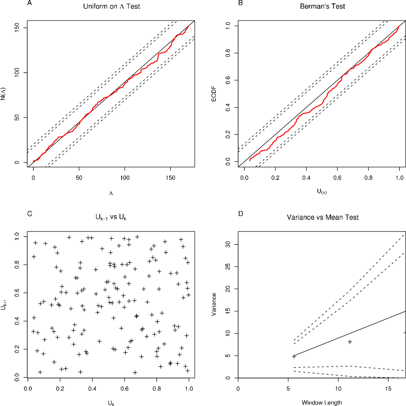
Figure 2: Four of the five Ogata’s tests applied to the simulated data of Fig. 1.

4 A new test based on Donsker’s Theorem: The Wiener Process Test

As we have seen in the previous section each Ogata’s test considered separately has some drawback. This is why Ogota used all of them in his paper [16]. It seems therefore reasonable to try to develop new tests which could replace part of Ogata’s tests and / or behave better than them in some conditions, like when the sample size is small. We are going to apply directly Donsker’s Theorem to our time transformed spike trains as an attempt to fulfill this goal.

Following Billingsley [1, p 121], we start by defining a functional space:

Definition of $D$

Let $D=D[0,1]$ be the space of real functions $x$ on $[0,1]$ that are right-continuous and have left-hand limits:

1. For $0\leq t<1$, $x(t+)=\lim_{s\downarrow t}x(s)$ exists and $x(t+)=x(t)$.

2. For $0\leq t<1$, $x(t-)=\lim_{s\uparrow t}x(s)$ exists.

Donsker’s Theorem

Given iid random variables $\xi_{1},\xi_{2},\ldots,\xi_{n},\ldots$ with mean 0 and variance $\sigma^{2}$ defined on a probability space $(\Omega,\mathcal{F},\mathrm{P})$. We can associate with these random variables the partial sums $S_{n}=\xi_{1}+\cdots+\xi_{n}$. Let $X^{n}(\omega)$ be the function in $D$ with value:

$$X^{n}_{t}(\omega)=\frac{1}{\sigma\sqrt{n}}S_{\lfloor nt\rfloor}(\omega)$$ (15)

at $t$, where $\lfloor nt\rfloor$ is the largest integer $\leq nt$. Donsker’s Theorem states that: The random functions $X^{n}$ converge weakly to $W$, the Wiener process on $[0,1]$.

See [1, pp 146-147] for a proof of this theorem.

Using Donsker’s Theorem

If our model is correct then the $\Lambda_{j+1}-\Lambda_{j}$ are iid random variables from an exponential distribution with rate 1. Since the mean and variance of this distribution are both equal to 1, if we define:

$$\xi_{j}=\Lambda_{j+1}-\Lambda_{j}-1$$ (16)

the $\xi_{j}$s should be iid with mean 0 and variance 1. Once we have observed the $\Lambda_{j}$s and therefore the $\xi_{j}$s we can built the realization of Eq. 15. The latter should “look like” a Wiener process on $[0,1]$. Notice that the realization of Eq. 15 is nearly the same as the function obtained by subtracting $N(\Lambda)$ from $\Lambda$ on Fig. 1 C, before dividing the abscissa by $n$ and the ordinate by $\sqrt{n}$ as illustrated on Fig. 3. This is also seen by looking at the expression of the partial sums in this particular case:

$$S_{n}=\Lambda_{n+1}-\Lambda_{1}-n$$ (17)

Figure 3: Illustration of the “mapping” to a Wiener process. A, The counting process has been subtracted from the integrated intensity of Fig. 1 C, on the transformed time scale. B, The corresponding realization of the $X^{n}_{t}$ function of Eq. 15.

The next element we need in order to get a proper test is a way to define a tight region of $[0,1]\times\mathbb{R}$ where, say, 95% of the realizations of a Wiener process should be. This turns out to be a non trivial but luckily solved problem. Kendall et al [12] have indeed shown that the boundaries of the tightest region containing a given fraction of the sample paths of a Wiener process is are given by a so called Lambert W function. They have moreover shown that this function can be very well approximated by a square root function plus an offset: $a+b\,\sqrt{t}$. We next need to find the $a_{\alpha}$ and $b_{\alpha}$ such that the realizations of a Wiener process are entirely within the boundaries with a probability $1-\alpha$. There is no analytical solution to this problem but efficient numerical solutions are available. Loader and Deely [13] have shown that the first passage time of a Wiener process through an arbitrary boundary $c(t)$ is the solution of a Volterra integral equation of the first kind. They have proposed a “mid-point” algorithm to find the first passage time distribution. Their method does moreover provide error bounds when $c(t)=a+b\,\sqrt{t}$. Then using the “symmetry” of the Wiener process with respect to the time axis we have to find $a_{\alpha}$ and $b_{\alpha}$ such that the probability to have a first passage $\leq 1$ is $\frac{\alpha}{2}$.

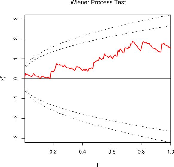
Figure 4: Illustration of the “Wiener process test”. The same graph as Fig. 3 B is shown with 95% and 99% boundaries appearing as dotted curves. The boundaries have the form: $a+b\,\sqrt{t}$, the coefficients are given in the text.

Using an integration step of 0.001 and, $a_{0.05}=0.299944595870772$, $b_{0.05}=2.34797018726827$, we get: $0.9499<P_{0.95}<0.9501$. Using $a_{0.01}=0.313071417065285$, $b_{0.01}=2.88963206734397$, we get: $0.98998<P_{0.99}<0.99002$. In the sequel we will refer to the comparison of the sample path of $X_{t}^{n}$ in Eq. 15 with boundaries whose general form is: $a_{\alpha}+b_{\alpha}\,\sqrt{t}$ as a Wiener process test.

Finite sample properties

We now estimate the empirical coverage probability of our two regions for a range of “realistic” sample sizes, from 10 to 900, using Monte Carlo simulations. The results from 10000 simulated “experiments” are shown on Fig. 5 A. The empirical coverage probability of the region with a nominal 95% confidence is at the nominal level across the whole range studied. The empirical coverage probability of the region with a nominal 99% confidence does slightly worse. The empirical coverage is roughly 98% for a sample size smaller than 100, 98.5% between 100 and 300 and reaches the nominal value for larger sample sizes. The overall performances of the test are surprisingly good given the simplicity of its implementation.

Since we are also interested in carrying out multiple testing using for instance Ogata’s first test, Berman’s test and our “Wiener process test”, we studied the dependence of false negatives under the three possible pairs formed from these three tests. The results are shown on Fig. 5 B. Here we see that Berman’s and Ogata’s first tests are independent (i.e., the empirical results are compatible with the hypothesis of independence). But neither of these tests is independent of the “Wiener process test” when a 95% confidence level (on each individual test) is used. In both cases (Berman and Ogata’s first test) when a trial is rejected at the 95% level it is less likely to be also rejected by the “Wiener process test”. If we combine the three tests at the 99% level and decide to reject the null hypothesis if any one of them is rejected, we obtain an empirical coverage probability of $\sim 0.96$ for a sample size between 10 and 100. Above this size the probability becomes $\sim 0.97$.

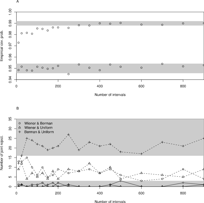
Figure 5: A, Empirical coverage probabilities of the 95 and 99% confidence regions for the Wiener test. Each dot on the graph was obtained from 10000 simulated “experiments”. Each experiment was made of a number, $n$, of draws given on the abscissa. Each draw was the realization of an exponential distribution with rate 1. The procedure described by applying Eq. 16 before Eq. 15 was then applied. The resulting step function was compared, at the steps locations with the boundaries values. The grey band correspond to 95% confidence bands for a binomial distribution with 10000 draws and a success probability of 0.95 (bottom) and 0.99 (top). B, Number of joint rejections of paired tests. Using the same simulations as in A, the number of joint rejection of the “Wiener process test” and of the “Berman’s test” (circles), of the “Wiener process test” and of the “Uniform test” (i.e., Ogata’s first test, triangles), of the “Berman’s test” and of the “Uniform test” (crosses) at the 95% level (dotted lines) and at the 99% level (continuous line). Gray areas, 95% confidence region for a binomial distribution with 10000 trials and a rejection probability of $0.05^{2}$ (top) and $0.01^{2}$ (bottom). The p values of the Kolmogorov statistic of the “Berman” and “Uniform” tests were obtained with the exact method of [14] and implemented in function ks.test of R.

A remark

It is clear from the hypothesis of Donsker’s theorem that the “Wiener process test” cannot replace Ogata’s second test (Berman’s test). As long as the distribution of the mapped intervals has the same first and second moments than an exponential distribution with rate 1, the data will pass the test.

5 Real data examples

We illustrate in this section the performances of the tests on real data. The data, like the software implementing the test and the whole analysis presented in this article are part of our STAR (Spike Train Analysis with R) package for the R software. The data were recorded extracellularly in vivo from the first olfactory relay of an insect, the cockroach, Periplaneta americana. Details about these recordings and associated analysis methods can be found in [4, 20]. The names of the data sets used in this section are the names used for the corresponding data in STAR. The reader can therefore easily reproduce the analysis presented here. We do moreover provide with STAR a meta-file [21, 7], called a vignette in R terminology, allowing the reader to re-run exactly the simulation / data analysis of this article.

5.1 Spontaneous activity data

Two examples of spike trains recorded during a period of 60 s of spontaneous activity are shown on Fig. 6. The spike trains appear as both a counting process sample path and as a “raster plot” on this figure. A renewal model was fitted with the maximum likelihood method to each train. The data from neuron 3 of data set e060517spont were fitted with an inverse-Gaussian model, while the ones of neuron 1 of data set e060824spont were fitted with a log logistic model. The spike times where transformed (Eq. 7) before applying Ogata’s test 1, 2, 3, 5 and the new Wiener test. The results are shown on Fig. 7.

Figure 6: Two actual spike trains. Each plot shows the counting process sample path ($N(t)$) associated with a train. The spikes density and their number are too high for the discontinuities of $N(t)$ to systematically appear. A "raster plot" is drawn at the bottom of each plot. A raster plot is a spike train representation where the occurrence time of each spike is marked by a tick (see [20] for details).

The time transformed spike train of neuron 3 of data set e060517spont passes Berman’s test (Fig. 7 A2) as well as Ogata’s third test (Fig. 7 A3) but fails to pass Ogata’s tests 1 and 5 (Fig. 7 A1 and A4) as well as the new Wiener process test (Fig. 7 A5). The time transformed spike train of neuron 1 of data set e060824spont passes Ogata’s first test (Fig. 7 B1) as well as Berman’s test (Fig. 7 B2), but fails Ogata’s tests 3 (Fig. 7 B3) and 5 (Fig. 7 B4) as well as the new Wiener process test (Fig. 7 B5).

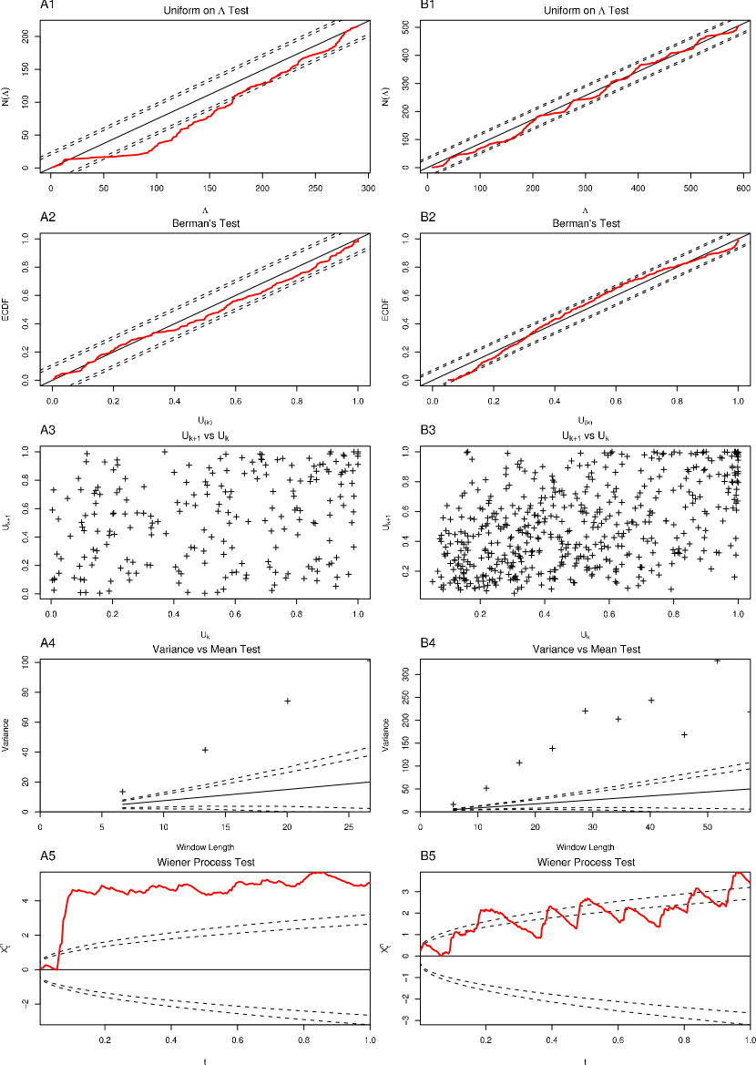
Figure 7: The tests applied after time transformation. A, neuron 3 from data set e060517spont fitted with an inverse-Gaussian renewal model. B, neuron 1 from data set e060824spont fitted with a log logistic renewal model. Notice that the tests are here applied directly to the data used to fit the model. The domains defined by the boundaries (dotted lines) have therefore not exactly their nominal coverage value.

5.2 Stimulus evoked data

The odor evoked responses of neuron 1 of data set e070528citronellal are illustrated here. This is the occasion to use a more sophisticated intensity model, albeit still a wrong one (see bellow). The “raw data” are shown on Fig. 8. An inhomogeneous Poisson model was fitted to trial 2 to 15 using a smoothing spline approach [8, 20]. This estimated time dependent intensity was then used to transform the spike times of the first trial. The tests are shown on Fig. 9. In this case the train contains 98 spikes making Ogata’s test 5 barely applicable (not shown on figure). Ogata’s test 3 (Fig. 9 C) is hard to interpret since with few spikes and a sparse filling of the graph, the presence or absence of a pattern is not obvious. Ogata’s test 1 (Fig. 9 A) and Berman’s test (Fig. 9 B) are passed but the Wiener process test (Fig. 9 D) is not.

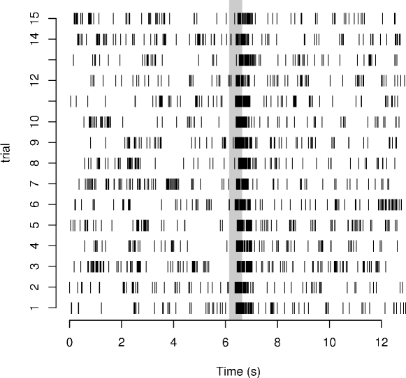
Figure 8: An example of odor evoked responses. Neuron 1 of data set e070528citronellal is used. 15 citronellal odor puffs were applied successively. Each puff was 0.5 long [4, 20] (the gray area corresponds to the opening time of the valve delivering the odor). Odor presentations were performed 1 mn apart. The spike trains of each trial are represented as raster plots. The first trial is at the bottom of the graph, the 15th on top.

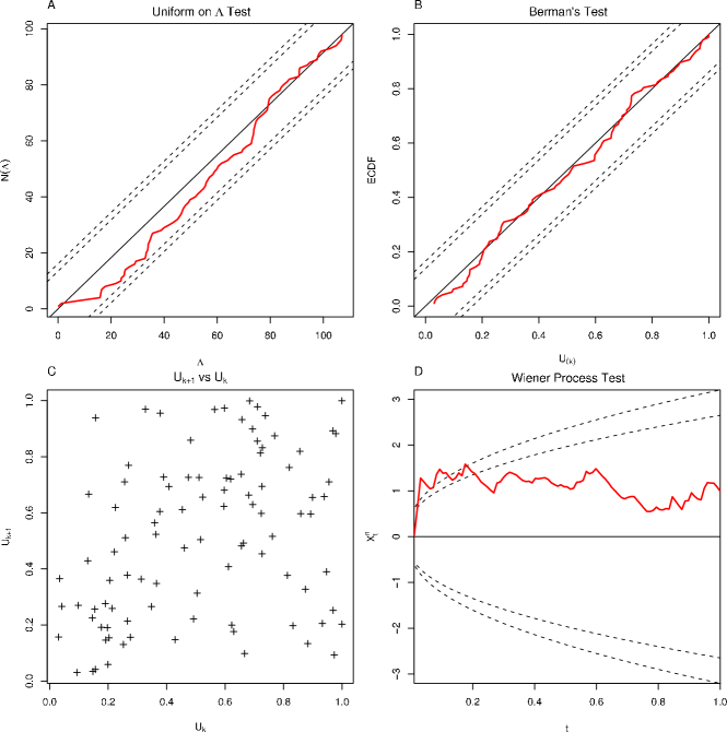
Figure 9: The tests applied after time transformation. An inhomogeneous Poisson model was fitted to trial 2 to 15 and used to transform the spike times of trial 1.

6 Conclusions

Ogata [16] introduced a tests battery for counting process models. He made moreover rather clear through his use of the tests that more than a single one of them should be used in practice. Brown et al [3] introduced in the neuroscience literature Berman’s test (Ogata’s second test) which has become the only test used (when any is used) in this field. We could also remark that only one case of a model fitted to real data actually passing this test has ever been published [3, Fig. 1A]. Clearly our examples of Fig. 7 A2 and B2 and of Fig. 9 B, would multiply this number by four. But we have to stick to Ogata’s implicit message. Our choice of examples reiterates this point showing cases where Berman’s test is passed. We do not want to imply that Berman’s test is a “bad” test but to warn the neuroscience community that misleading conclusions can be obtained when only this test is used.

We have also introduced the “Wiener process test” a direct application of Donsker’s Theorem to the time transformed spike trains. The test is simple to implement (Eq. 16 and 15) and exhibits good finite sample properties (Fig. 5). It is clearly not a replacement for the Ogata’s tests battery but a complement (Fig. 7 and 9). It’s finite sample properties make it particularly useful in situations were a small number of spikes makes the interpretation of Ogata’s tests 3 and 5 potentially ambiguous (Fig. 9).

References

- [1] Patrick Billingsley. Convergence of Probability Measures. Wiley - Interscience, 1999.
- [2] D. R. Brillinger. Maximum likelihood analysis of spike trains of interacting nerve cells. Biol Cybern, 59(3):189–200, 1988.
- [3] Emery N Brown, Riccardo Barbieri, Valérie Ventura, Robert E Kass, and Loren M Frank. The time-rescaling theorem and its application to neural spike train data analysis. Neural Comput, 14(2):325–346, Feb 2002. Available from: http://www.stat.cmu.edu/~kass/papers/rescaling.pdf.
- [4] Antoine Chaffiol. Étude expérimentale de la représentation des odeurs dans le lobe antennaire de Periplaneta americana. PhD thesis, Université Paris XIII, 2007. Available at: http://www.biomedicale.univ-paris5.fr/physcerv/C_Pouzat/STAR_folder/The%seAntoineChaffiol.pdf.
- [5] E. S. Chornoboy, L. P. Schramm, and A. F. Karr. Maximum likelihood identification of neural point process systems. Biol Cybern, 59(4-5):265–275, 1988.
- [6] D. R. Cox and P. A. W. Lewis. The Statistical Analysis of Series of Events. John Wiley & Sons, 1966.
- [7] Robert Gentleman and Duncan Temple Lang. Statistical Analyses and Reproducible Research. Working Paper 2, Bioconductor Project Working Papers, 29 May 2004. Available at: http://www.bepress.com/bioconductor/paper2/.
- [8] Chong Gu. Smoothing Spline Anova Models. Springer, 2002.
- [9] D.H. Johnson. Point process models of single-neuron discharges. J. Computational Neuroscience, 3(4):275–299, 1996.
- [10] Don H. Johnson and Ananthram Swami. The transmission of signals by auditory-nerve fiber discharge patterns. J. Acoust. Soc. Am., 74(2):493–501, August 1983.
- [11] R. E. Kass and V. Ventura. A spike-train probability model. Neural Comput., 13(8):1713–1720, 2001. Available from: http://www.stat.cmu.edu/~kass/papers/imi.pdf.
- [12] W.S. Kendall, J.M. Marin, and C.P. Robert. Brownian Confidence Bands on Monte Carlo Output. Statistics and Computing, 17(1):1–10, 2007. Preprint available at: http://www.ceremade.dauphine.fr/%7Exian/kmr04.rev.pdf.
- [13] C. R. Loader and J. J. Deely. Computations of boundary crossing probabilities for the Wiener process. J. Statist. Comput. Simulation, 27(2):95–105, 1987.
- [14] George Marsaglia, Wai Wan Tsang, and Jingbo Wang. Evaluating Kolmogorov’s Distribution. Journal of Statistical Software, 8(18):1–4, 11 2003.
- [15] Y. Ogata. On lewis’ simulation method for point processes. IEEE Transactions on Information Theory, IT-29:23–31, 1981.
- [16] Yosihiko Ogata. Statistical Models for Earthquake Occurrences and Residual Analysis for Point Processes. Journal of the American Statistical Association, 83(401):9–27, 1988.
- [17] Murat Okatan, Matthew A. Wilson, and Emery N. Brown. Analyzing Functional Connectivity Using a Network Likelihood Model of Ensemble Neural Spiking Activity. Neural Computation, 17(9):1927–1961, September 2005.
- [18] D. H. Perkel, G. L. Gerstein, and G. P. Moore. Neuronal spike trains and stochastic point processes. I the single spike train. Biophys. J., 7:391–418, 1967. Available from: http://www.pubmedcentral.nih.gov/articlerender.fcgi?tool=pubmed&pubmedi%d=4292791.
- [19] D. H. Perkel, G. L. Gerstein, and G. P. Moore. Neuronal spike trains and stochastic point processes. II simultaneous spike trains. Biophys. J., 7:419–440, 1967. Available from: http://www.pubmedcentral.nih.gov/articlerender.fcgi?tool=pubmed&pubmedi%d=4292792.
- [20] Christophe Pouzat and Antoine Chaffiol. Automatic spike train analysis and report generation. an implementation with R, R2HTML and STAR. Submitted manuscript. Pre-print distributed with the STAR package: http://cran.at.r-project.org/web/packages/STAR/index.html, 2008.
- [21] Anthony Rossini and Friedrich Leisch. Literate Statistical Practice. UW Biostatistics Working Paper Series 194, University of Washington, 2003.
- [22] Wilson Truccolo and John P. Donoghue. Nonparametric modeling of neural point processes via stochastic gradient boosting regression. Neural Computation, 19(3):672–705, 2007. Available at: http://donoghue.neuro.brown.edu/pubs/Truccolo_and_Donoghue_Neural_Comp_%2007.pdf.
- [23] Wilson Truccolo, Uri T. Eden, Matthew R. Fellows, John P. Donoghue, and Emery N. Brown. A Point Process Framework for Relating Neural Spiking Activity to Spiking History, Neural Ensemble and Extrinsic Covariate Effects. J Neurophysiol, 93:1074–1089, February 2005. Available at: http://jn.physiology.org/cgi/content/full/93/2/1074.