Steady-state distribution function for a gas of independent electrons far from equilibrium

Abstract

The quasi-stationary nonequilibrium distribution function of an independent electron gas interacting with a medium, which is at local thermal equilibrium, can be obtained by entropy production rate minimization, subject to constraints of fixed moments. The result is not restricted to the region near equilibrium (linear response) and provides a closure of the associated generalized hydrodynamic equations of the electron gas for an arbitrary number of moments. Besides an access to far from equilibrium states, the approach provides a useful description of semi-classical transport in mesoscopic conductors, particularly because macroscopic contacts can be naturally taken into account.

Introduction - Electron transport in matter is often described by the Boltzmann transport equation (BTE) for the distribution function $f$, from which the (semi-classical) transport properties can be calculated Ziman1967 . Kohler Kohler1948 proved that the stationary solution of the linearized BTE satisfies a variational principle for the entropy production rate, which has been widely used to determine linear transport coefficients Ziman1967 ; Kohler1949 ; Sondheimer1950 ; Martyushev2006 . Schlup Schlup1975 and Jones Jones1983 gave arguments for the validity of Kohler’s principle beyond linear response. Note that a linear BTE does in general not imply a restriction to the near-equilibrium, i.e., linear response, region. First, provided the linearity is not due to linearization of a nonlinear BTE, the linear BTE may be valid for large deviations from equilibrium. Secondly, because forces appear as coefficients of a term linear in $f$, the resulting currents are generally nonlinear functions of the forces. Below, a method is introduced that provides $f$ as a function of its moments by minimization of the total entropy production rate. The result is not restricted to the near-equilibrium case (i.e., to linear response), and serves as a closure of generalized hydrodynamic equations for the moments. Recently, it has been shown that an analogous method applied to a photon gas in matter at local thermal equilibrium, where the BTE is exactly linear, describes nonequilibrium radiation satisfactorily well also far from equilibrium ChristenKassubek2009 .
After introducing the method, a few examples will be discussed, including metallic and nonmetallic electric conduction, and low-frequency transport in mesoscopic conductors.

Basic formulation of the problem - Consider electrons in $d$($=1,2,3$)-dimensional space, with space and velocity vectors ${\bf x}$ and ${\bf v}$, respectively. They may interact with a medium at local thermal equilibrium, such that the electron distribution function $f({\bf x},{\bf v})$ obeys the linear BTE Ziman1967 ,

$$\partial_{t}f+{\bf v}\cdot{\bm{\nabla}}_{x}f+{\bf a}\cdot{\bm{\nabla}}_{v}f=\mathcal{L}(f_{0}-f)\;\;.$$ (1)

The force $m\,{\bf a}=e\,{\bm{\nabla}}_{x}U$ acting on the particles with effective mass $m$ and electron charge $-e$, is related to the gradient of the electric potential $U({\bf x})$, which may be determined later (on the hydrodynamic level) self-consistently from the Poisson equation. The positive definite and self-adjoint linear (integral-) operator $\mathcal{L}$ describes the interaction of the electrons with the medium. The terms $-\mathcal{L}f$ and $\mathcal{L}f_{0}$ can be interpreted, respectively, as absorption of electrons and emission of electrons equilibrated with respect to the medium (e.g., traps, contacts in mesoscopic systems, etc.), which has local temperature $T$ and (electro-)chemical potential $\mu$. The index $0$ indicates the Fermi equilibrium distribution $f_{0}=\{\exp(\frac{H-\mu}{kT})+1\}^{-1}$, where $H(v)$ is the particle energy, $v=\mid{\bf v}\mid$, and $k$ is the Boltzmann constant. Equation (1) applies to a large class of systems in solid state physics Ziman1967 , presumes micro-reversibility, and is usually solved within linear response, i.e., in first order of $\delta f=f-f_{0}$. Typical standard methods are the BGK approximation BathnagarGrossKrook1954 , or Kohler’s variational approach with the help of trial functions. However, if the linearity is not due to a linearization of a nonlinear scattering term but remains valid for larger deviations of $f$ from $f_{0}$, a nonlinear (far from equilibrium) solution is apposite. Note that particle number conservation is generally not assumed, which allows for carrier absorption and emission by the medium (see examples below).
To derive a quasi-steady state solution for general $f$, an arbitrary number $M+1$ of moments are defined:

$$n({\bf x}) = \left(\frac{m}{h}\right)^{d}\int d^{d}v\,f({\bf x},{\bf v})$$ (2)

$${\bf j}({\bf x}) = \left(\frac{m}{h}\right)^{d}\int d^{d}v\,{\bf v}f({\bf x},{\bf v})$$ (3)

$$\Pi_{kl}({\bf x}) = \left(\frac{m}{h}\right)^{d}\int d^{d}v\,v_{k}v_{l}f({\bf x},{\bf v})$$ (4)

etc., where $h$ is Planck’s constant (spin degeneracy can be included later). Equations for $M$ moments follow from multiplication of Eq. (1) by $1$, $v_{k}$, $v_{k}v_{l}$, …, and velocity integration:

$$\partial_{t}n+{\bm{\nabla}}\cdot{\bf j} = P^{(n)}$$ (5)

$$\partial_{t}{\bf j}+{\bm{\nabla}}\cdot\Pi-n{\bf a} = {\bf P}^{(j)}\;\;$$ (6)

etc. ($k,l=1,...,d$). The highest order moment and the terms on the right hand side, $P^{(n)}=(m/h)^{d}\int d^{d}v\mathcal{L}(f_{0}-f)$, ${\bf P}^{(j)}=(m/h)^{d}\int d^{d}v{\bf v}\mathcal{L}(f_{0}-f)$, etc., are functionals of the unknown distribution $f$. In order to close the $M$ moment equations, we will calculate $f$ from entropy production rate minimization, subject to constraints of $M$ fixed moments, given by Eqs. (2), (3), etc.. The distribution and derived quantities will thus depend on them.

Determination of $f$ - It is important to consider the total entropy production rate of the whole isolated system, which consists of two contributions associated with the independent electron gas and with the medium acting as an equilibrium bath. The first part, $\dot{s}_{F}$, can be derived from the entropy density $s_{F}({\bf x})=-k\left(\frac{m}{h}\right)^{d}\int d^{d}v\{f\ln f+(1-f)\ln(1-f)\}$ by differentiation of $s_{F}$ with respect to time, replacement of $\partial_{t}f$ with the help of Eq. (1), partial $v$-integration, and finally writing the result as an entropy balance equation, $\partial_{t}s_{F}+{\bm{\nabla}}\cdot{\bf q}_{s_{F}}=\dot{s}_{F}$, with entropy current density ${\bf q}_{s_{F}}$. This gives $\dot{s}_{F}=k\left(\frac{m}{h}\right)^{d}\int d^{d}v\;\ln\left(\frac{f}{1-f}\right)\mathcal{L}(f-f_{0})$. The second part, $\dot{s}_{B}=W/T$, associated with the medium, is obtained from the heat power density $W=\left(\frac{m}{h}\right)^{d}\int d^{d}v\;(H-\mu)\;\mathcal{L}(f-f_{0})$. The relation $H-\mu=kT\ln(1/f_{0}-1)$ implies $\dot{s}_{B}=k\left(\frac{m}{h}\right)^{d}\int d^{d}v\ln\left(\frac{1-f_{0}}{f_{0}}\right)\mathcal{L}(f-f_{0})$. The total entropy production rate, $\dot{s}_{B}+\dot{s}_{F}$, is

$$\dot{s}=k\left(\frac{m}{h}\right)^{d}\int d^{d}v\;\ln\left(\frac{f(1-f_{0})}{f_{0}(1-f)}\right)\mathcal{L}(f-f_{0})\;.$$ (7)

The distribution function $f$ is then determined by the variational principle $\delta\dot{s}/\delta f=0$ subject to the constraints Eqs. (2), (3), … of fixed moments. This is the main result, and provides a closure for the generalized hydrodynamics of the independent electron gas far from local equilibrium and for an arbitrary number of moments.

Two-moment closure - For illustration, consider $M=2$ moments and assume $\mathcal{L}(f_{0}-f)=r(v)(f_{0}-f)$ with $v$-dependent relaxation rate $r$. An example beyond this relaxation-time approximation will an elastic scatterer in the last example. Optimization of Eq. (7) with constraints (2) and (3) leads to

$$r(v)\left(\ln\frac{f(1-f_{0})}{f_{0}(1-f)}+\frac{f-f_{0}}{f(1-f)}\right)=\lambda^{(n)}+{\bm{\lambda}}^{(j)}\cdot{\bf v}\;\;$$ (8)

with Lagrange parameters $\lambda^{(n)}$ and ${\bm{\lambda}}^{(j)}$. It is readily checked that the optimization problem is convex, which ensures that the solution is a constraint minimum. Solving Eq. (8) for $f$ and elimination of the Lagrange parameters provides $f({\bf v};n,{\bf j})$ and then $P^{(n)},{\bf P}^{(j)}$, and $\Pi_{kl}$.

Weak Nonequilibrium - Expansion with respect to $\delta f=f-f_{0}$ gives $\delta f=f_{0}(1-f_{0})(\lambda^{(n)}+{\bm{\lambda}}^{(j)}\cdot{\bf v})/2r$. Elimination of $\lambda^{(n)}$ and ${\bm{\lambda}}^{(j)}$ with the help of Eqs. (2) and (3) leads to $P^{(n)}=r^{(n)}(n_{0}-n)$ and ${\bf P}^{(j)}=-r^{(j)}{\bf j}$ with

$$r^{(n)} = \frac{\int d^{d}v\,f_{0}(1-f_{0})}{\int d^{d}v\,r^{-1}(v)f_{0}(1-f_{0})}$$ (9)

$$r^{(j)} = \frac{\int d^{d}v\,v^{2}f_{0}(1-f_{0})}{\int d^{d}v\,v^{2}r^{-1}(v)f_{0}(1-f_{0})}\;\;,$$ (10)

For $d=3$, Eq. (10) gives the usual linear response relaxation-time mobility, $e/mr^{(j)}$ Ziman1967 . The stress tensor, $\Pi_{kl}$, stays diagonal and isotropic, and deviates from equilibrium $\Pi_{0,kk}$ by

$$\Delta\Pi_{kk}=\frac{(n-n_{0})}{d}\frac{\int d^{d}v\;v^{2}r^{-1}f_{0}(1-f_{0})}{\int d^{d}v\;r^{-1}f_{0}(1-f_{0})}\;\;.$$ (11)

Note that $f_{0}(1-f_{0})=-\frac{kT}{mv}\partial_{v}f_{0}$, and Eqs. (9)-(11) simplify in the low temperature limit for $\mu=mv_{F}^{2}/2>0$, because $\partial_{v}f_{0}$ is a Dirac $\delta$-function at the equilibrium Fermi velocity $v_{F}=h(n_{0}/\Omega_{d})^{1/d}/m$ (with $\Omega_{1}=2$, $\Omega_{2}=\pi$, $\Omega_{3}=4\pi/3$). For $T\to 0$, $\Pi_{0,kl}=\delta_{kl}n_{0}v_{F}^{2}/(d+2)$. Finite temperature corrections may be considered in terms of $\gamma=2kT/mv^{2}_{F}$, in the same way as done by other standard methods for weak nonequilibrium.

Fermi Sphere, Zero Temperature - For $\mu>0$ and $T\to 0$, Eq. (8) can be solved analytically for strong deviation from equilibrium. After multiplying Eq. (8) by $f(1-f)$, using $(1-f_{0})/f_{0}=\exp(m(v^{2}-v_{F}^{2})/2kT)$ and the fact that $f\in[0,1]$, one can solve the resulting equation with an expansion $f=f^{(0)}+\gamma f^{(1)}+O(\gamma^{2})$. One concludes for $\gamma\to 0$ that $f^{(0)}=1$ and $f^{(0)}=0$ if $\eta({\bf v}):=m(v^{2}-v_{F}^{2})/2kT-\lambda^{(n)}/r-{\bm{\lambda}}^{(j)}\cdot{\bf v}/r$ is negative and positive, respectively (note $\lambda^{(n,j)}\propto 1/\gamma$). Hence, $\eta({\bf v})=0$ defines the boundary of the nonequilibrium Fermi surface for $T\to 0$. For $v$-independent $r$, the Fermi sphere is shifted according to ${\bf j}/n$ and resized according to $n/n_{0}$ as one expects, and the stress tensor becomes

$$\Pi_{kl}=\frac{h^{2}}{5m^{2}}\frac{n^{1+2/d}}{(d+2)\Omega_{d}^{2/d}}\,\delta_{kl}+\,\frac{j_{k}j_{l}}{n}\;\;,$$ (12)

in accordance with the usual expression of the hydrodynamic momentum flux tensor. A factor $2$ in $\Omega_{d}$ must be included for spin degeneracy; for instance, Eq. (12) leads then to the $d=3$ electron gas pressure introduced by Bloch Bloch1933 .
For $v$-dependent $r$ these results change in general far from equilibrium. As an example, consider $r(v)=r_{0}v_{F}/v$ with constant $r_{0}$. For $1d$, one finds $P^{(n)}=n_{0}r_{0}\ln\sqrt{(n/n_{0})^{2}-(j/nv_{F})^{2}}$ and $r^{(j)}=r_{0}n_{0}/n$. The divergence of $P^{(n)}$ at $j=v_{F}n^{2}/n_{0}$ is an artifact due to the specific $r(v)$ and occurs when the shifted Fermi ‘surface’ approaches $v=0$. From $P^{(n)}(n,j)=0$ and Eq. (6) one can derive the relation between $j$ and the electric field. A simple experimental test of the theory would be based on a measurement of the nonlinear current-voltage characteristics of a nano-wire on an appropriate support material, if the associated wire-support interaction in terms of $r(v)$ is known.
A non-spherical deformation of the Fermi sphere for varying current can occur in $d>1$. For illustration, we have calculated the deformed Fermi circle in $d=2$ for $r(v)=r_{0}v_{F}/v$. By comparing the result (solid thick curve in Fig. 1) with a Fermi circle for constant $r$ (dashed curve), one observes that the former is closer to the equilibrium distribution for low $v$-values and further away for larger $v$-values. This reflects the stronger equilibration, induced by the entropy principle ChristenKassubek2009 , at low $v$ for this $r(v)$. It is clear from Eq. (4), that not only the shift but also the deformation of the Fermi sphere gives a contribution to an anisotropy $\Pi_{kl}$.

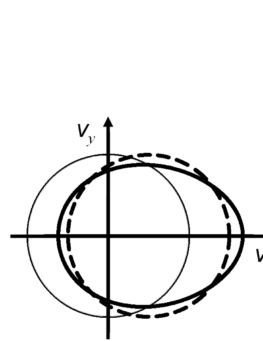
Figure 1: Far from equilibrium Fermi circle in $2d$ for $n=n_{0}$ and $j=n_{0}v_{F}/2$ in $x$-direction for constant $r$ (dashed) and deformed circle for $r\propto 1/v$ (solid). The thin line refers to equilibrium.

Energy Gap, $3d$, Finite Temperature - Consider now $\mu<0$, such that $f_{0}\approx N\exp(-mv^{2}/2kT)\ll 1$, with $N=\exp(\mu/kT)$, describes a dilute, non-degenerate, equilibrium electron gas in an insulator material. The terms $-rf$ and $rf_{0}$ describe trapping and emission of thermally equilibrated electrons from electron traps, respectively. The non-equilibrium distribution is calculated for a step function-like rate $r(v)=r_{1}$ for $v$ $\ll v_{T}:=\sqrt{kT/m}$ and $r(v)=r_{2}=0.1\,r_{1}$ for $v$ $\gg v_{T}$, which models a mobility edge (inset in Fig. 2). The resulting distribution function $f$ is shown in Fig. 3 for three different cases. Again, in $v$-regions of larger scattering rates $r(v)$, $f$ is closer to $f_{0}$ because equilibration is stronger. The effective rate $r^{(j)}(n,j)$, far from equilibrium, as a function of the current density $j$ (with ${\bf j}=j\hat{e}_{z}$ in $z$-direction) is shown for different values of $n$ in Fig. 2. The near equilibrium result, $r^{(j)}(n_{0},j=0)=0.306\,r_{1}$ can be obtained directly from Eq. (10). For large currents, $j\gg n_{0}v_{T}$, as one expects $r^{(j)}\to r_{2}$. It is clear that an additional consideration of higher order moments will allow to describe hot electrons.

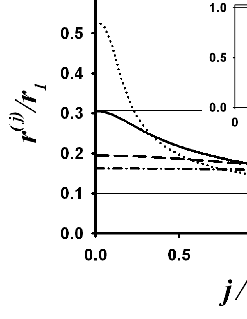
Figure 2: Mean rate $r^{(j)}/r_{1}$ as a function of $j$ for $r(v)$ shown in the inset; dotted: $n/n_{0}=0.6$; solid: $n/n_{0}=1$; dashed: $n/n_{0}=1.4$; dashed-dotted: $n/n_{0}=1.8$. Near equilibrium (upper thin line): $r^{(j)}=0.306r_{1}$; lower thin line: $r_{2}/r_{1}=0.1$.

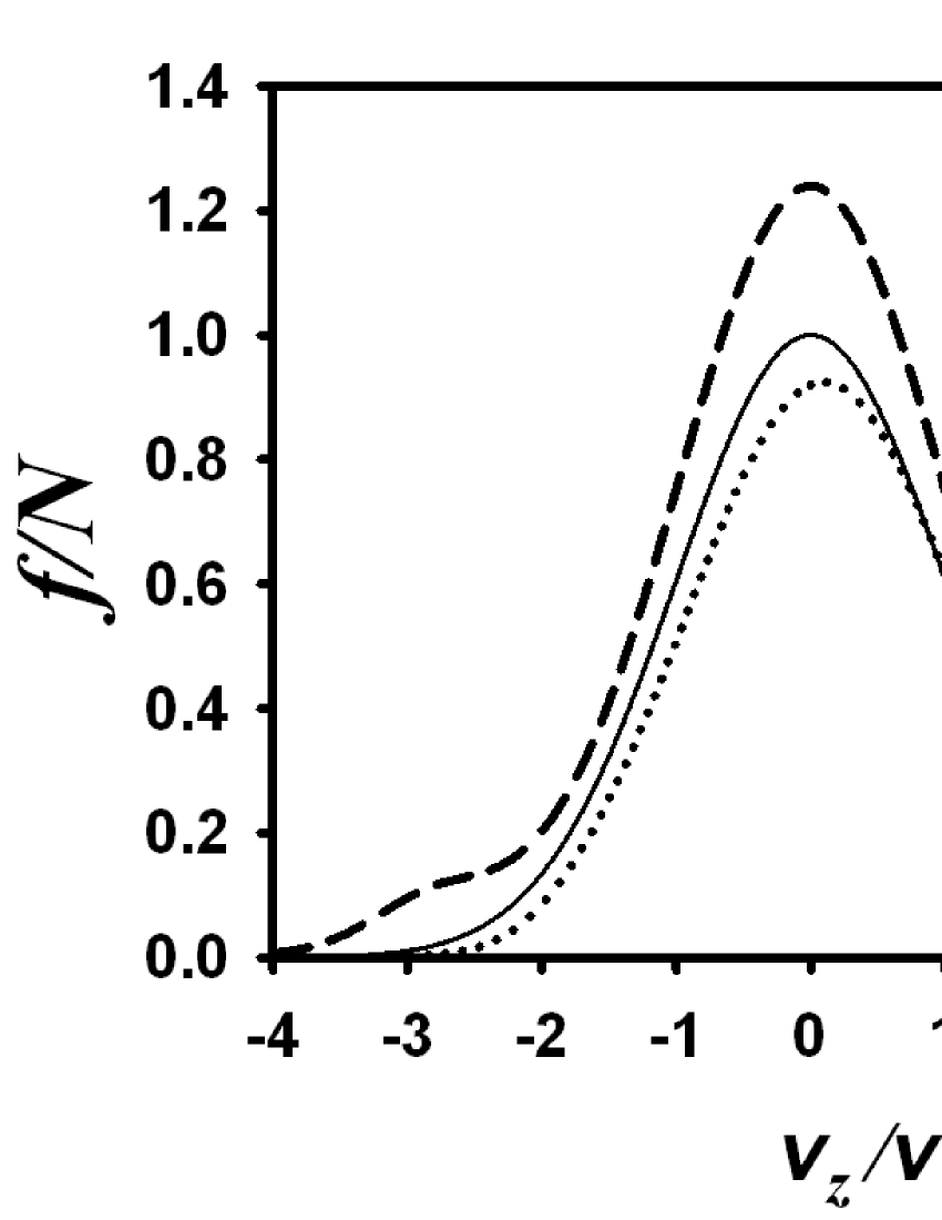
Figure 3: Distribution as a function of $v$ in current direction (arrow in inset). Solid: equilibrium $f=f_{0}$; dashed: $j=0$, $n=2n_{0}$; dotted $n=n_{0}$, $j=n_{0}v_{T}/2$. Inset: $f$-contour for $n=n_{0}$, $j=n_{0}v_{T}/2$. Tail regions with lower $r(v)$ (weaker equilibration) show stronger nonequilibrium.

Low frequency admittance of a 1d wire - The generalized hydrodynamics framework is very useful to describe low-frequency transport in mesoscopic conductors. To illustrate this, the admittance of the one-dimensional symmetric wire shown in Fig.4 is calculated. The contacted long end pieces are described by a finite $r\equiv r_{c}$, which models in a natural way contacts to macroscopic electron reservoirs, where carriers from the wire are absorbed ($-r_{c}f$) and equilibrated carriers are emitted ($r_{c}f_{0}$) into the wire. For $-L/2<x<L/2$ the electrons are supposed to move ballistic, except for a localized elastic scatterer at $x=0$ with transmission probability ${\cal T}=1-{\cal R}$. Hence, $\mathcal{L}(f_{0}-f)=\nu\delta(x)v_{F}(f(-v)-f(v))$ in $-L/2<x<L/2$ with $\nu={\cal R}/{\cal T}$.
Since the purpose is to illustrate the principle, the discussion is restricted to linear response (cf. BriggsLeburton1989 ). Coulomb interaction can be included self-consistently ChristenButtiker1996 . We assume negligible capacitive coupling between the contacts, small contact impedance between the substrate and the contacted wire pieces, and obviously disregard electron-electron interaction effects like Luttinger liquid formation Yacoby1996 or thermal conductance decrease Rechetal2009 .
The low-frequency admittance, $G=G_{0}-i\omega E$, for an applied voltage $\Delta V\exp(-i\omega t)$, with $\Delta V=V_{1}-V_{2}$, includes the DC conductance, $G_{0}$, and the emittance, $E$ ChristenButtiker1996 ; Gabelli2007 .

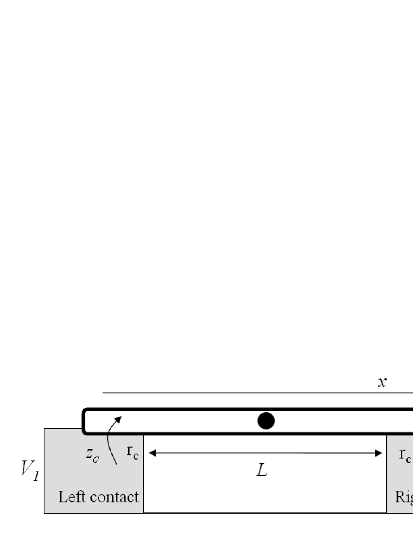
Figure 4: Quantum wire connected to two electrodes at temperature $T$ and potentials $V_{1,2}$, with contact impedance per length, $z_{c}$, and scattering rate $r=r_{c}$. The ballistic region ($r\to 0$) of length $L$, contains a localized elastic scatterer with transmission probability ${\cal T}$.

The linearized hydrodynamic equations (5)-(6) can be written as

$$v_{F}\kappa\Delta n+\partial_{x}j = 0$$ (13)

$$\kappa j+v_{F}\partial_{x}\Delta n = \frac{2e}{h}\partial_{x}U-2\nu\delta(x)j\;\;,$$ (14)

where $\partial_{x}$ denotes the spatial derivative, $\Delta n=n-n_{0}$, and $\kappa=(r-i\omega)/v_{F}$ with $r=r(v_{F})$. By virtue of $v_{F}=hn_{0}/2m$, $n_{0}$ was eliminated. The applied voltage is equal to the total difference in the electro-chemical potential, $V=U-hv_{F}n/2e$. The electrical behavior of the wire-support contact is modeled by a phenomenological contact impedance $z_{c}$ with $-ez_{c}\partial_{x}j=V_{1,2}-U(x)$ on the two sides.
In order to derive $G$, we integrate Eq. (14) from $x=-\infty$ to $x=\infty$ and obtain with $\Delta V=V_{1}-V_{2}$, $I(x)=-ej$, and $\kappa_{c}=(r_{c}-i\omega)/v_{F}$:

$$\frac{e^{2}}{h}\Delta V=\int_{-\infty}^{-L/2}\kappa_{c}I(x)\,dx+(\nu-\frac{i\omega L}{2})I(0),$$ (15)

where the symmetry of the wire was used. The current in the wire in the left contact region $x<-L/2$ must decay, hence $j\propto\exp(\beta x)$ there, with $\beta=(\kappa_{c}^{-2}+2e^{2}z_{c}/h\kappa_{c})^{-1/2}$ that follows from Eqs. (13) and (14). After evaluation of the integral in Eq. (15) one obtains $e^{2}\Delta V/hI(0)=1+\nu+e^{2}z_{c}\kappa_{c}/h-i\omega L/2v_{F}$. With $1+\nu=1/{\cal T}$ and $z_{c}\to 0$, the low frequency admittance $G=I(0)/\Delta V$ becomes $G=\frac{2e^{2}}{h}{\cal T}+i\omega\frac{D}{4}{\cal T}^{2}$ with $D=4e^{2}L/hv_{F}$, where factors of $2$ for two spin states are included. This result is in accordance with Ref. ChristenButtiker1996 in the considered limit case of vanishing capacitance between the contacts. $V(x)$ in the ballistic wire regions has the meaning of a quasi Fermi-level, and the local entropy production rate $\dot{s}(x)=mr(I^{2}+v_{F}e\Delta n^{2})/Tn_{0}e^{2}$ is localized in the contact regions. A generalization to ballistic electrons in arbitrary geometries and arbitrarily far from equilibrium is straight-forward; it requires higher order (multipole) moments in $d>1$, similar to a $P-N$ approximation in (non-diffusive) radiation SiegelHowell1992 . The generalized hydrodynamic equations with the discussed closure may serve as a general footing for simulations of nano-electronics devices in the full range between diffusive and ballistic transport.

Conclusion - It is also straight-forward to extend the method to other than parabolic energy-momentum relations and to generalized moments Struchtrup1998 . For instance, it should be possible to treat in a similar way massless Fermions like neutrinos in stars or electric conduction in graphene, if these particles are independent and the particle-medium interaction can be modeled by $\mathcal{L}(f_{0}-f)$.
Acknowledgement - The author thanks Frank Kassubek for his valuable contributions.

References

- (1) J. M. Ziman, Electrons and Phonons (Clarendon Press, Oxford, 1967); Can. J. Phys., 34, 1256 (1956).
- (2) M. Kohler, Z. Phys. 124, 772 (1948).
- (3) M. Kohler, Z. Phys. 125, 679 (1949).
- (4) E. H. Sondheimer, Proc. Roy. Soc. A 203, 75 (1950).
- (5) L. M. Martyushev and V. D. Seleznev, Phys. Rep. 426, 1 (2006).
- (6) W. A. Schlup, J. Math. Phys. 16, 1733 (1975).
- (7) W. Jones, J. Phys. A: Math. Gen. 16, 3629 (1983).
- (8) T. Christen and F. Kassubek, J. Quant. Spectr. Rad. Transf. 110, 452 (2009).
- (9) P. L. Bhatnagar, E. P. Gross, and M. Krook, Phys. Rev. 94, 511 (1954).
- (10) F. Bloch, Z. Phys. 81, 363 (1933).
- (11) S. Briggs and J. P. Leburton, Phys. Rev. B 39, 8025 (1989).
- (12) T. Christen and M. Büttiker, Phys. Rev. Lett. 77, 143 (1996).
- (13) A. Yacoby et al. Phys. Rev. Lett. 77, 4612 (1996).
- (14) J. Rech, T. Micklitz, and K. A. Matveev, Phys. Rev. Lett. 102, 116402 (2009).
- (15) J. Gabelli et al., Phys. Rev. Lett. 98, 166806 (2007).
- (16) R. Siegel and J. R. Howell, Thermal radiation heat transfer, (Hemisphere Publ. Corp., Washington, 1992).
- (17) H. Struchtrup, Annals of Physics 266, 1 (1998).