Long-range disassortative correlations in generic random trees

Abstract

We explicitly calculate the distance dependent correlation functions in a maximal entropy ensemble of random trees. We show that correlations remain disassortative at all distances and vanish only as a second inverse power of the distance. We discuss in detail the example of scale-free trees where the diverging second moment of the degree distribution leads to some interesting phenomena.

Published in: Phys. Rev. E 81, 041136 (2010). PACS numbers: 05.90.+m, 89.75.Hc, 05.10.–a

I Introduction

The knowledge of correlations is important and interesting for any system. Looking from the practical point of view correlation means additional information: if two quantities are correlated, the knowledge of one of them implies certain information about the other one. In physical systems correlations usually indicate interactions between parts of the system. The prototypical example is given by the Ising spin system where the nearest-neighbors interactions induce long-range correlations leading to a phase transition.

The situation in random graphs is somewhat different. It is known that for random geometries even in the absence of any explicit terms inducing interactions between vertices their degree may be correlated bs ; b1 ; b2 ; b3 ; Satorras2001 ; msz ; pn ; bo ; kim . Moreover, those correlations are long-range, i.e., they fall off as some power of distance bs ; b1 ; b2 ; b3 . They are generated by model constraints rather than by explicit interactions. It should be also stressed that the distance dependent correlation functions in the ensemble of random graphs are much more complicated objects than their fixed lattice counterparts bs ; b2 . To see that let us take some generic correlation function on random graphs

$$\left\langle\sum_{i,j}A({q_{i}})B({q_{j}})\,\delta_{l,|i-j|}\right\rangle,$$ (1)

where $q_{i}$ denotes the degree of the vertex $i$, i.e., the number of branches emerging from it. $A$ and $B$ are some arbitrary functions depending on the vertex degree and $|i-j|$ is the graph (geodesic) distance between vertices $i$ and $j$. For random geometry it makes no sense in general to choose two fixed points—that is why we sum over all the pairs of points on the graph. The graph distance is the length of the shortest path between those two vertices and as such it is dependent on the whole graph. That means that the above expression is not a two-point function but a highly nonlocal object. That is a fundamental difference between random and fixed geometries.

In this paper, we study in detail correlations between degrees of vertices as a function of distance. We consider an ensemble of all labeled trees ${\mathcal{T}}(V)$ with a fixed number of vertices $V$, on which we define the probability measure

$$P(T)\equiv\Omega_{V}^{-1}\frac{1}{V!}\prod_{i\in T}w_{q_{i}}.$$ (2)

$\Omega_{V}$ denotes the partition function of this ensemble (normalization factor) and $q_{i}$ is the degree of vertex $i$; $w_{q}$’s $(q>0)$ are some non-negative numbers (weights). This is a maximal-entropy ensemble with a given degree distribution (see Appendix). An important property of the measure (2) is that it factorizes into a product of one-point measures, so it does not introduce any explicit correlations. This means that any observed correlations arise from the fact that we consider a specific set of graphs and not from the measure itself.

We show that the connected degree-degree correlations are not zero and fall off with the distance as $l^{-2}$

$$\bar{\pi}^{con}_{q,r}(l) = \bar{\pi}_{q,r}(l)-\bar{\pi}_{q}(l)\bar{\pi}_{r}(l)$$ (3)

$$= -\frac{(q-2)(r-2)}{\left[2+(\left\langle q^{2}\right\rangle-4)(l-1)\right]^{2}}\,\pi_{q}\pi_{r}.$$

Here $\bar{\pi}_{q,r}(l)$ is the joint probability that two vertices distance $l$ apart will have degrees $q$ and $r$, respectively. Those correlations are disassortative. The average degree of the distance $l$ neighbors of a vertex with degree $q$ decreases

$$\bar{k}_{l}(q)=2+\frac{\left\langle q^{2}\right\rangle-4}{q+(\left\langle q^{2}\right\rangle-4)(l-1)}.$$ (4)

For $l=1$ this reduces to the results obtained in Ref. kim . In the following sections we provide the detailed definitions of the quantities introduced above and derive those results. We will also discuss what happens for the scale-free trees when $\left\langle q^{2}\right\rangle$ diverges.

The paper is organized as follows: Sec. II introduces some basic definitions concerning correlations in random trees. Then we derive the vertex degree distribution using the field theory approach in Sec. III and proceed on in Sec. III.1 calculating the distance dependent correlation functions. Two examples of Erdös-Rényi and scale-free trees are given in Secs. III.2 and III.3, respectively. In the following Sec. III.4 the results for scale-free trees are verified using Monte Carlo (MC) simulations. Final discussion and summary of our results are given in Sec. IV.

II Correlations

For each graph we introduce

$$n_{q,r}(l)\equiv\sum_{i,j\in G}\delta_{q_{i},q}\delta_{q_{j},r}\delta_{|i-j|,l},$$ (5)

which is the number of pairs of points with degrees $q$ and $r$ separated by the distance $l$. We define two further quantities: the number of pairs at the distance $l$ with one end point of specified degree

$$n_{q}(l)\equiv\sum_{r}n_{q,r},$$ (6)

and the number of all pairs of vertices at the distance $l$

$$n(l)\equiv\sum_{q,r}n_{q,r}(l).$$ (7)

If we want to define the joint probability $\pi_{q,r}(l)$ we have two obvious choices. The first one is

$$\pi_{q,r}(l)\equiv\left\langle\frac{n_{q,r}(l)}{n(l)}\right\rangle_{n(l)\neq 0},$$ (8)

where the subscript denotes that we restrict the average to the ensemble of graphs for which $n(l)$ is not zero. The second possibility is to use

$$\bar{\pi}_{q,r}(l)\equiv\frac{\left\langle n_{q,r}(l)\right\rangle}{\left\langle n(l)\right\rangle}.$$ (9)

In Ref. bo we have argued that the first quenched definition is more natural in the context of random graphs. However, it is much more difficult to work with. In this paper we will assume that the ensemble of generic trees is self-averaging and the two above definitions are equivalent. For a more detailed discussion of this issue we refer to bo . Similarly we define

$$\bar{\pi}_{q}(l)\equiv\frac{\left\langle n_{q}(l)\right\rangle}{\left\langle n(l)\right\rangle},$$ (10)

and the connected two point probability

$$\bar{\pi}^{con}_{q,r}(l)\equiv\bar{\pi}_{q,r}(l)-\bar{\pi}_{q}(l)\,\bar{\pi}_{r}(l).$$ (11)

We further define the connected correlation function bs ; b1 ; b2

$$\pi^{con}_{\bar{q},\bar{r}}(l)\equiv\sum_{q,r}q\,r\,\bar{\pi}^{con}_{q,r}(l).$$ (12)

Finally we define average degree of the vertices at the distance $l$ from a vertex of degree $q$ as follows:

$$\bar{k}_{l}(q)\equiv\frac{\left\langle n_{q,\bar{r}}(l)\right\rangle}{\left\langle n_{q}(l)\right\rangle},$$ (13)

where

$$n_{q,\bar{r}}(l)\equiv\sum_{r}r\,n_{q,r}.$$ (14)

III Generic random trees

We consider an ensemble of all labeled trees with the probability measure (2). The partition function $\Omega_{V}$ is defined as the sum of the weights of all the trees in the ensemble

$$\Omega_{V}\equiv\frac{1}{V!}\sum_{T\in\mathcal{T}(V)}\prod_{i\in T}w_{q_{i}}.$$ (15)

The partition function of the corresponding grand-canonical ensemble is defined by the discrete Laplace transform

$$\Omega(\mu)=\sum_{V=1}^{\infty}e^{-\mu V}\Omega_{V}.$$ (16)

We will use the field theory approach to calculate it jk . We define the function

$$W(\mu)\equiv\int\text{d}\phi\exp\left[N\left(-\frac{1}{2}\phi^{2}+e^{-\mu}\sum_{q=0}\frac{w_{q}}{q!}\phi^{q}\right)\right].$$ (17)

Its formal perturbative expansion in $e^{-\mu}$ will generate Feynman’s diagrams with desired weights and symmetry factors (for an introduction see any textbook on field theory, e.g., Refs. bdfn and ift or Ref. graphs ). This expansion will, however, contain all the graphs including those which are not connected or contain loops. We can restrict the expansion to connected graphs only by considering the function $\log W(\mu)$. To obtain just the tree graphs we will use the expansion in $N^{-1}$. According to Feyman’s rules for the expression (17) each edge in the graph introduces a factor $N^{-1}$ and each vertex a factor $N$ which together contribute $N^{-E+V}$, where $E$ is the number of edges in the graph. If $L$ is the number of independent loops in the graph then $E-V=L-1$, so the first term of the $N^{-1}$ expansion will group graphs with no loops, the second one graphs with one loop, and so on.

That means that the contribution of tree graphs is given by the first term in the saddle-point approximation. The saddle-point equation is

$$\frac{\text{d}}{\text{d}\phi}\left(-\frac{1}{2}\phi^{2}+e^{-\mu}\sum_{q=0}^{\infty}\frac{w_{q}}{q!}\phi^{q}\right)=0.$$ (18)

We will denote by $Z(\mu)$ the solution of the above equation and rewrite it as

$$Z(\mu)=e^{-\mu}\sum_{q=1}^{\infty}\frac{w_{q}}{(q-1)!}Z^{q-1}=e^{-\mu}\frac{F\left(Z(\mu)\right)}{Z(\mu)},$$ (19)

where

$$F(Z)\equiv\sum_{q=1}^{\infty}\frac{w_{q}}{(q-1)!}Z^{q}.$$ (20)

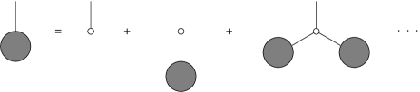
Figure 1: Graphical representation of Eq. (19). Each gray bubble corresponds to the sum over planted trees given by the partition function $Z(\mu)$. Branches without a vertex (small empty circle) at one end denote a stem.

Inserting Eq. (19) into Eq. (17) and taking the logarithm to keep only connected graphs we obtain

$$\begin{split}\Omega(\mu)&=e^{-\mu}\sum_{q=0}^{\infty}\frac{w_{q}}{q!}Z^{q}(\mu)-\frac{1}{2}Z^{2}(\mu).\end{split}$$ (21)

It is easy to check that

$$e^{-\mu}Z(\mu)=\frac{\partial\Omega(\mu)}{\partial w_{1}}.$$ (22)

Figure 1 shows a graphical interpretation of $Z(\mu)$: it is the partition function of the ensemble of planted trees . Planted trees are the trees with a stem attached to one of the vertices. Its properties and resulting critical behavior were calculated in Refs. adfo ; bb ; jk .

Figure 2: Graphical representation of Eq. (23) and the singularity of $Z(\mu)$.

The model has two main phases. In the so called generic or tree phase the the function $F(Z)/Z^{2}$ has a minimum inside its domain (see Fig. 2) and so Eq. (19), which can be rewritten as

$$e^{\mu}=\frac{F(Z)}{Z^{2}},$$ (23)

does not have any solution for $\mu<\mu_{0}$. The function $Z(\mu)$ has a singularity at $\mu_{0}$ given by the condition for the minimum

$$2F(Z_{0})=Z_{0}F^{\prime}(Z_{0}),\quad\text{and}\quad\mu_{0}=\log\frac{F(Z_{0})}{Z^{2}_{0}}.$$ (24)

At this singularity the partition function behaves like

$$Z(\mu)\approx Z_{0}-Z_{1}\sqrt{\mu-\mu_{0}}+Z_{2}(\mu-\mu_{0}),$$ (25)

regardless of the form of the weights $w_{q}$. In this contribution we will limit our self to this phase only. Inserting the expansion (25) into Eq. (19) and expanding to the order $\Delta\mu\equiv\mu-\mu_{0}$ ($Z_{2}$ cancels in the resulting equation) we obtain

$$\frac{Z_{0}^{2}}{Z^{2}_{1}}=\frac{1}{2}\frac{F^{\prime\prime}(Z_{0})Z_{0}^{2}}{F(Z_{0})}-1.$$ (26)

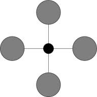
Figure 3: Graphical representation of the partition function $\Omega(q,\mu)$ given by Eq. (27) for $q=4$. Each gray bubble corresponds to the sum over planted trees given by the partition function $Z(\mu)$; the smaller black circle represents the root which contributes a weight factor $e^{-\mu}w_{4}$; the additional $\frac{1}{4!}$ factor comes from the fact that the relative position of branches in the compound tree is irrelevant.

The vertex degree distribution of this model was calculated using the correspondence with the balls in boxes model in Ref. bbj . Here we rederive it using a different method which can be easily extended to the case of two-point correlations studied in Ref. b3 . Let us denote by $\Omega(q;\mu)$ the partition function of the rooted grand-canonical ensemble of trees with the condition that the degree of the root is $q$. Then

$$\begin{split}\Omega(q;\mu)=w_{q}\frac{\partial\Omega(\mu)}{\partial w(q)}=e^{-\mu}\frac{w_{q}}{q!}Z^{q}(\mu).\end{split}$$ (27)

The graphical interpretation of this equation is shown in Fig. 3. The sought degree distribution is proportional to the canonical partition function $\Omega_{V}(q)$. Inserting the expansion (25) into Eq. (27) we obtain

$$\Omega(q;\mu) \approx e^{\mu_{c}}e^{\Delta\mu}\frac{w_{q}}{q!}Z_{0}^{q}\left(1-q\frac{Z_{1}}{Z_{0}}\sqrt{\Delta\mu}\right)$$ (28)

$$\approx e^{\mu_{c}}e^{\Delta\mu}\frac{w_{q}}{q!}Z_{0}^{q}\exp\left(-q\frac{Z_{1}}{Z_{0}}\sqrt{\Delta\mu}\right).$$

The last expression has a known inverse Laplace transform

$$e^{-a\sqrt{\Delta\mu}}\;\xleftrightarrow{\text{Lap.}}\;\frac{1}{2\sqrt{\pi}}\,\frac{a}{V^{\frac{3}{2}}}\;e^{-\frac{a^{2}}{4V}},$$ (29)

so finally keeping only the first terms in the $V^{-1}$ expansion and fixing the normalization we obtain the formula

$$\pi(q)=\frac{1}{F(Z_{0})}\;\frac{w_{q}Z_{0}^{q}}{(q-1)!}.$$ (30)

Using the above formula we can give an interpretation of the right-hand side of Eq. (26)

$$\frac{1}{2}\frac{F^{\prime\prime}(Z_{0})Z_{0}^{2}}{F(Z_{0})}-1 = \frac{1}{2}\frac{\sum_{q=1}\frac{q(q-1)}{(q-1)!}w_{q}Z_{0}^{q}}{F(Z_{0})}-1$$ (31)

$$= \frac{1}{2}\sum_{q=1}q(q-1)\pi(q)-1$$

$$= \frac{1}{2}\left(\left\langle q^{2}\right\rangle-4\right).$$

Here we have used the fact that on trees the average degree $\left\langle q\right\rangle=2$ (in the large $V$ limit). Please note that

$$\left\langle q^{2}\right\rangle-4=\left\langle(q-2)^{2}\right\rangle\geq 0.$$ (32)

The $\left\langle q^{2}\right\rangle$ is equal to $4$ only in the $\omega_{1}\rightarrow 0$ limit.

III.1 Correlations in generic random trees

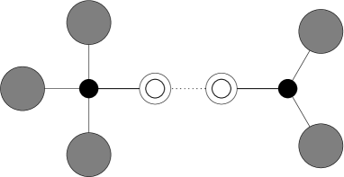
Figure 4: Graphical representation of the partition function $\Omega_{l}(q,r;\mu)$ given by Eq. (33) for $q=4$ and $r=3$. Gray bubbles correspond to the partition function $Z(\mu)$ and the smaller black circles mark the vertices with degrees $q$ and $r$; double circles represent the $l-1$ vertices along the path connecting them in which we sum over all possible insertions of the $Z(\mu)$ function (see Fig. 5).

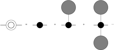
Figure 5: Double circles denote the summation over all possible insertions of the $Z(\mu)$ function (gray bubbles).

We proceed as in the previous section but this time we introduce a partition function $\Omega_{l}(q,r;\mu)$ of all the trees with two points marked, such that the points are at the distance $l$ and have degrees $q$ and $r$, respectively. Because we are considering the trees there is exactly one path linking the two marked vertices (see Fig. 4). As in the previous section we can express the partition function $\Omega_{l}(q,r;\mu)$ by $Z(\mu)$ b2 ; adj

$$\Omega_{l}(q,r;\mu) = \frac{e^{-\mu}w_{q}}{(q-1)!}\;Z^{q-1}(\mu)\frac{e^{-\mu}w_{r}}{(r-1)!}\;Z^{r-1}(\mu)$$ (33)

$$\times \left[e^{-\mu}\sum_{k=2}\frac{w_{k}}{(k-2)!}\;Z^{k-2}\right]^{l-1}.$$

The last term comes from the vertices along the path for which we have to sum up all the possible insertions of the $Z(\mu)$ function (see Fig. 5). This summation can be done in the following way:

$$e^{-\mu}\sum_{q=2}\frac{w_{q}}{(q-2)!}\;Z^{q-2} = e^{-\mu}\frac{\partial}{\partial Z}\sum_{q=1}\frac{w_{q}}{(q-1)!}\;Z^{q-1}$$ (34)

$$= e^{-\mu}\frac{\partial}{\partial Z}\frac{F(Z)}{Z}.$$

Differentiating Eq. (19) with respect to $\mu$ we come to the relation

$$Z^{\prime}(\mu)\left(1-e^{-\mu}\frac{\partial}{\partial Z}\frac{F(Z)}{Z}\right)=-Z.$$ (35)

Using it we finally obtain

$$\begin{split}e^{-\mu}\sum_{q=2}\frac{w_{q}}{(q-2)!}\;Z^{q-2}=1+\frac{Z(\mu)}{Z^{\prime}(\mu)}.\end{split}$$ (36)

Inserting into Eq. (33) first the above formula and then the expansion (25) we get

$$\Omega_{l}(p,q;\mu)\approx\frac{w_{q}}{(q-1)!}\,\frac{w_{r}}{(r-1)!}\;Z_{0}^{q+r-2}$$

$$\times\left(1-\frac{Z_{1}}{Z_{0}}\sqrt{\Delta\mu}\right)^{q+r-2}\left(1-2\frac{Z_{0}}{Z_{1}}\sqrt{\Delta\mu}\right)^{l-1}.$$ (37)

This can be further approximated by

$$\Omega_{l}(p,q;\mu) \approx \frac{w_{q}}{(q-1)!}\,\frac{w_{r}}{(r-1)!}\;Z_{0}^{q+r-2}$$ (38)

$$\times e^{-\left[\frac{Z_{1}}{Z_{0}}(q+r-2)+2\frac{Z_{0}}{Z_{1}}(l-1)\right]\sqrt{\Delta\mu}},$$

and using Eq. (29) we obtain to the leading order in $V$

$$\left\langle n_{qr}\right\rangle\propto\Omega_{l}(p,q;V) \approx \frac{w_{q}}{(q-1)!}\,\frac{w_{r}}{(r-1)!}\;Z_{0}^{q+r-2}$$

$$\times \left[\frac{Z_{1}}{Z_{0}}(q+r-2)+2\frac{Z_{0}}{Z_{1}}(l-1)\right].$$

Finally, we get

$$\bar{\pi}_{q,r}(l)= \,\pi_{q}\pi_{r}\frac{(q+r-2)+\left(\left\langle q^{2}\right\rangle-4\right)(l-1)}{2+\left(\left\langle q^{2}\right\rangle-4\right)(l-1)},$$ (40)

$$\bar{\pi}_{q}(l)= \,\pi_{q}\frac{q+\left(\left\langle q^{2}\right\rangle-4\right)(l-1)}{2+\left(\left\langle q^{2}\right\rangle-4\right)(l-1)}.$$ (41)

Inserting this into Eqs. (11) and (13) we obtain the results (3) and (4). Summing up Eq. (3) over $q$ and $r$ we get the connected correlation function (12)

$$\begin{split}\bar{\pi}^{con}_{\bar{q},\bar{r}}(l)=-\frac{\left[\left\langle q^{2}\right\rangle-4\right]^{2}}{\left[2+(\left\langle q^{2}\right\rangle-4)(l-1)\right]^{2}}.\end{split}$$ (42)

III.2 Example 1

In the first example we put $w_{q}=1$, so all the trees in the ensemble have the same weight. In this case $F(Z)=Ze^{Z}$. The solution of Eq. (24) is $Z_{0}=1$ from which follows:

$$\pi_{q}=\frac{1}{e}\frac{1}{(q-1)!},\quad\left\langle q^{2}\right\rangle=\sum_{q=1}^{\infty}\frac{1}{e}\frac{q^{2}}{(q-1)!}=5.$$ (43)

leading to

$$\bar{\pi}_{q}(l) =\pi_{q}\frac{q+l-1}{1+l},$$ (44)

$$\bar{\pi}^{con}_{q,r}(l) =-\frac{1}{e^{2}}\frac{(q-2)(r-2)}{(l+1)^{2}}\frac{1}{(q-1)!}\frac{1}{(r-1)!},$$ (45)

and

$$\bar{\pi}^{con}_{\bar{q},\bar{r}}(l)=-\frac{1}{(l+1)^{2}},\quad\bar{k}_{l}(q)=2+\frac{1}{q+l-1}.$$ (46)

III.3 Example 2: Scale-free trees

In this example we choose $w_{q}=q^{-\beta}(q-1)!$ which corresponds to the planar graphs studied in Refs. adfo and bb . Then $F(Z)$ is given by the polylogarithm function $\operatorname{Li}_{\beta}(Z)$

$$F(Z)=\sum_{q=1}^{\infty}\frac{Z^{q}}{q^{\beta}}\equiv\operatorname{Li}_{\beta}(Z).$$ (47)

and Eq. (24) takes the form $2\operatorname{Li}_{\beta}(Z_{0})=\operatorname{Li}_{\beta-1}(Z_{0})$. It has the solution for $\beta<\beta_{C}$ with $\beta_{C}\approx 2.4788$ given by $2\zeta(\beta_{C})=\zeta(\beta_{C}-1)$. At the critical value of $\beta=\beta_{C}$ the partition function no longer scales as in Eq. (25) and in principle we cannot use the Laplace transform Eq. (29) anymore. However, as shown in Ref. bepw the large $V$ behavior is not changed and we expect our formula to hold in the large $V$ limit. From Eq. (30) we read-off the degree distribution

$$\pi(q)=\frac{q^{-\beta}Z_{0}^{q-1}}{F(Z_{0})}.$$ (48)

At the critical value of $\beta$, $Z_{0}=1$ and the vertex degree distribution is scale free. The average

$$\left\langle q^{2}\right\rangle=2+\frac{1}{\operatorname{Li}_{\beta}(Z_{0})}\left[\operatorname{Li}_{\beta-2}(Z_{0})-\operatorname{Li}_{\beta-1}(Z_{0})\right],$$ (49)

diverges as $\beta\rightarrow\beta_{C}$. Formula (3) leads for $l>1$ to

$$\lim_{V\rightarrow\infty}\bar{\pi}^{con}_{q,r}(l)=0.$$ (50)

This would imply that the correlations vanish in the large $V$ limit. However, this limit (50) is not uniform. It is easy to check that the integrated correlation functions do not disappear

$$\lim_{V\rightarrow\infty}\bar{\pi}^{con}_{\bar{q},\bar{r}}(l)=-\frac{1}{(l-1)^{2}},$$ (51)

and

$$\lim_{V\rightarrow\infty}\bar{k}_{l}(q)=2+\frac{1}{l-1}.$$ (52)

Please note that the above results are universal and valid for any kind of scale-free trees with $\beta<3$.

III.4 Monte Carlo simulations

The results obtained in the previous sections are valid only in the strict $V\rightarrow\infty$ limit and it is clear that for finite $V$ our formulas will not hold for any $l$. Defining the average distance on a graph

$$\left\langle l\right\rangle=\sum_{l}l\frac{n(l)}{V^{2}},$$ (53)

we may expect that the formulas will be valid only for $l\ll\left\langle l\right\rangle$. The scaling of $\left\langle l\right\rangle$ with the graph size depends on the Hausdorff’s dimension $d_{H}$

$$\left\langle l\right\rangle\sim V^{{1}/{d_{H}}}.$$ (54)

For generic trees considered here $d_{H}=1/2$. For scale-free trees considered in example 2 we expect

$$d_{H}=\frac{1}{\gamma},\qquad\gamma=\frac{\beta_{C}-2}{\beta_{C}-1},$$ (55)

which gives $d_{H}\approx 3$. In the case of scale-free trees the volume dependence manifests itself by the cutoff in the degree distribution $\pi_{q}$ as well bck .

Expecting finite size effects to be more severe in the scale-free trees, we checked the $V$ dependence performing MC simulations of the ensemble described in the example 2. We have used an algorithm similar to “baby-universe surgery” abbjp . The basic move consisted of picking up an edge at random and cutting it. Then the smaller of the two resulting trees was grafted on some vertex of the bigger one. The most time consuming part of the algorithm was to find which tree was smaller. To save time the two trees were traversed simultaneously until one of them was filled completely. Additionally, to pick the attachment point from the bigger tree efficiently, the vertices of the trees were marked during the traversal. This move was supplemented with moves consisting of cutting up leaf nodes and attaching them to some other parts of the tree. This was much faster as it did not require traversing the tree. However, the autocorrelation time for such moves alone was much higher, especially for the scale-free trees. Because those trees are at the phase transition between the generic and the crumpled phase bb the autocorrelation time is high even for the tree grafting algorithm.

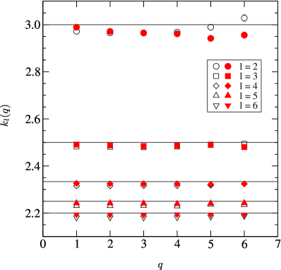
Figure 6: Average degree of distance $l$ neighbors $k_{l}(q)$ for $l=2$ to $6$ and trees with 64 000 (empty symbols) and 128 000 (filled symbols) vertices. Each symbol denotes different $l$; straight lines are the predictions given by Eq. (52).

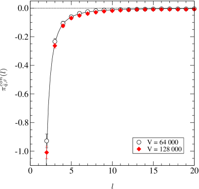
Figure 7: Connected correlation function $\pi_{\bar{q},\bar{r}}^{con}(l)$ for scale-free trees with 64 000 (empty circles) and 128 000 (filled diamonds) vertices. The solid line represents the prediction given by Eq. (51).

We have simulated trees of the size up to 128 000 vertices. To verify to which extent the ensemble is self-averaging we measured the quenched quantities which we then compared to our predictions. In Fig. 6 we have plotted the measured

$$k_{l}(q)=\left\langle\frac{n_{q,\bar{r}}(l)}{n_{q}(l)}\right\rangle,$$ (56)

as a function of $q$ for various values of $l$. Please note the large finite size effects for $l=2$. This is to be expected: For finite $V$ the $\left\langle q^{2}\right\rangle$ is also finite and actually grows slowly with $V$ bck . For larger $l$ the agreement with our results is quite good. Figure 7 shows the quenched correlation function

$$\pi^{con}_{\bar{q},\bar{r}}(l)=\left\langle\frac{n_{\bar{q},\bar{r}}(l)}{n(l)}\right\rangle-\left\langle\frac{n_{\bar{q}}(l)}{n(l)}\right\rangle^{2},$$ (57)

which is also well reproduced by our results.

IV Summary and Discussion

The appearance of the long-range correlations in generic trees is puzzling. Usually we expect the powerlike (scale-free) behavior to be manifested in systems at the criticality. The trees studied here apart from the scale-free example are, however, not critical. The free-energy density can be calculated in the infinite volume limit and remains an analytic function of the weights $\omega_{q}$ bb ; bbj . It has been also shown that the critical behavior in random trees is not associated with the diverging correlation length bbju . The correlations described here are thus of the structural and not of dynamical origin. A possible mechanism explaining it was proposed in Refs. b1 and bo : in connected graphs vertices of degree one must have neighbors of degree greater than one. It remains, however, to be understood how this effect can be propagated to larger distances.

Appendix A Maximal entropy

For each choice of the weights $w_{q}$ and a given number of vertices $V$ the ensemble (2) has a well defined degree distribution $\pi(q)$. Asymptotically for large $V$ this distribution is given by Eq. (30). Ref. BauerBernard contains a proof that the probability measure (2) has maximal entropy among all the measures producing the distribution $\pi(q)$. Here we repeat their arguments for completeness.

We start with an expression for the entropy plus the necessary Lagrange multipliers to force the constraints

$$\cal{S} = -\frac{1}{V!}\sum_{T\in\mathcal{T}}P(T)\log P(T)+\frac{\lambda}{V!}\sum_{T\in\mathcal{T}}P(T)$$ (58)

$$+\sum_{q=1}^{V}\frac{\lambda_{q}}{V!}\left(\sum_{T\in\mathcal{T}}n_{q}(T)P(T)-\pi(q)V\right).$$

Differentiating the above with respect to $P(T)$ we get

$$\log P(T)=\lambda-1+\sum_{q}\lambda_{q}n_{q}(T),$$ (59)

leading to

$$P(T)=e^{\lambda-1}\prod_{q}e^{\lambda_{q}n_{q}(T)}.$$ (60)

Putting

$$e^{\lambda-1}=\frac{\Omega_{V}}{V!},\quad\text{and}\quad e^{\lambda_{q}}=w_{q}$$ (61)

we obtain Eq. (2). We will now prove that this measure is a unique solution of Eq. (58) satisfying the constraints, at least in the $V\rightarrow\infty$ limit. Let us assume that we have another set of weights $\tilde{w}_{q}$ that produces the same probability distribution $\pi(q)$ (30)

$$\pi(q)=\frac{1}{F(Z_{0})}\frac{w_{q}Z_{0}^{q}}{(q-1)!}=\frac{1}{F(\tilde{Z}_{0})}\frac{\tilde{w}_{q}\tilde{Z_{0}}^{q}}{(q-1)!}.$$ (62)

It follows that:

$$\tilde{w}_{q}=\frac{F(\tilde{Z}_{0})}{F(Z_{0})}\left(\frac{Z_{0}}{\tilde{Z}_{0}}\right)^{q}\;w_{q},$$ (63)

hence

$$\prod_{i\in T}\tilde{w}_{q_{i}} = \prod_{i\in T}\frac{F(\tilde{Z}_{0})}{F(Z_{0})}\left(\frac{Z_{0}}{\tilde{Z}_{0}}\right)^{q_{i}}w_{q_{i}}$$ (64)

$$= \left(\frac{F(\tilde{Z}_{0})}{F(Z_{0})}\right)^{V}\left(\frac{Z_{0}}{\tilde{Z}_{0}}\right)^{\sum_{i\in T}q_{i}}\prod_{i\in T}w_{q_{i}}.$$

But this gives identical probability measure to Eq. (2) because of the condition $\sum_{i\in T}q_{i}=2V-2$ valid for each tree $T$.

References

- (1) B. V. de Bakker and J. Smit, Nucl. Phys. B 454, 343 (1995).
- (2) P. Bialas, Phys. Lett. B 373, 289 (1996).
- (3) P. Bialas, Nucl. Phys. B, Proc. Suppl. 53, 739 (1997).
- (4) P. Bialas, Nucl. Phys. B 575, 645 (2000).
- (5) R. Pastor-Satorras, A. Vasquez, and A. Vespignani, Phys. Rev. Lett. 87, 258701 (2001).
- (6) S. Maslov, K. Sneppen, and A. Zaliznyak, Physica A 333, 529 (2004).
- (7) J. Park and M. E. J. Newman, Phys. Rev. E 68, 026112 (2003).
- (8) P. Bialas and A. K. Oleś, Phys. Rev. E 77, 036124 (2008).
- (9) J. Kim, B. Kahng, and D. Kim, Phys. Rev. E 79, 067103 (2009).
- (10) J. J. Binney, N. J. Dowrick, A. J. Fisher, and M. E. J. Newman, The Theory of Critical Phenomena (Oxford University Press, Oxford, 1993).
- (11) P. Cvitanović, Field Theory, Nordita Lecture Notes (1983); http://chaosbook.org/FieldTheory
- (12) D. Bessis, C. Itzykson, and J.-B. Zuber, Adv. Appl. Math. 1, 109 (1980).
- (13) J. Ambjorn, B. Durhuus, J. Frohlich, and P. Orland, Nucl. Phys. B 270, 457 (1986).
- (14) J. Jurkiewicz and A. Krzywicki, Phys. Lett. B 392, 291 (1997).
- (15) P. Bialas and Z. Burda, Phys. Lett. B 384, 75 (1996).
- (16) P. Bialas, Z. Burda, and D. Johnston, Nucl. Phys. B 493, 505 (1997).
- (17) J. Ambjorn, B. Durhuus, and T. Jonsson, Phys. Lett. B 244, 403 (1990).
- (18) Z. Burda, J. Erdman, B. Petersson, and M. Wattenberg, Phys. Rev. E 67, 026105 (2003).
- (19) Z. Burda, J. D. Correia, and A. Krzywicki, Phys. Rev. E 64, 046118 (2001).
- (20) J. Ambjorn, P. Bialas, J. Jurkiewicz, Z. Burda, and B. Petersson, Phys. Lett. B 325, 337 (1994).
- (21) P. Bialas, Z. Burda, and J. Jurkiewicz, Phys. Lett. B 421, 86 (1998).
- (22) M. Bauer and D. Bernard, e-print arXiv:cond-mat/0206150.