Entanglement of Coarse Grained Quantum Field in the Expanding Universe

Abstract

We investigate the entanglement of a quantum field in the expanding universe. By introducing a bipartite system using a coarse-grained scalar field, we apply the separability criterion based on the partial transpose operation and numerically calculate the bipartite entanglement between separate spatial regions. We find that the initial entangled state becomes separable or disentangled after the spatial separation of two points exceed the Hubble horizon. This provides the necessary condition for the appearance of classicality of the quantum fluctuation. We also investigate the condition of classicality that the quantum field can be treated as the classical stochastic variables.

I Introduction

Inflation provides the mechanism to generate the seed fluctuation which leads to the formation of the large scale structure in our present Universe. During the accelerated expansion stage of the inflationary universe, short wavelength quantum fluctuations of the inflaton field are generated by particle creations and then they becomes longwavelength fluctuations larger than the Hubble horizon by the cosmic expansion. The generated longwavelength fluctuations are considered as the classical fluctuations responsible for the origin of structure in our Universe. The important question is how such quantum fluctuations change to classical fluctuations; quantum fluctuations must acquire the classical stochastic nature and transfer to classical density perturbations which lead to the gravitational instability to form the nonlinear structure in the Universe. We must explain what kind of mechanism causes such a quantum to classical transition of primordial fluctuationsGuthAH:PRD32:1985 ; SakagamiM:PTP79:1988 ; BrandenbergerRH:MPLA5:1990 ; NambuY:PL276B:1992 ; AlbrechtA:PRD50:1994 ; PolarskiD:CQG13:1996 ; LesgourguesJ:NPB497:1997 ; KieferC:CQG15:1998 .

In this paper, we aim to investigate this problem from the view-point of the quantum correlation, entanglement. The entanglement is the specific nature of the quantum system. When we calculate a correlation function of observables, we have a possibility that the correlation function cannot be reproduced using a classical probability distribution function if the system is entangled and the classical locality is violated EinsteinA:PR47:1935 ; BellJS:P1:1964 . Thus, we cannot regard the quantum fluctuations as the classical stochastic fluctuations as long as the system is entangled. If the quantum fluctuation becomes classical, the entanglement must be lost. We consider the entanglement of the quantum field between two spatially separated regions in the expanding universe and investigate how the quantum fluctuation acquires the classical nature during inflation. For the quantum field to behave as the classical stochastic field, it is necessary to lose the quantum correlation and the classical distribution function must appear. The entanglement property for the general $N$-partite system is complicated and we do not have a general tool to treat such a system. For a bipartite system, however, we have the necessary and sufficient conditions for the existence of quantum correlation (entanglement) PeresA:PRL77:1996 ; HorodeckiP:PLA232:1997 ; SimonR:PRL84:2000 ; DuanL:PRL84:2000 and apply this criterion to our problem.

In our previous work NambuY:PRD78:2008 , we investigated the behavior of the entanglement of the quantum field using a lattice model of a scalar field. We considered the entanglement between spatially separated two blocks and found that the bipartite entanglement between these two blocks is lost after their separation exceeds the horizon length. We also discussed that the disappearance of the entanglement yields only the necessary condition for the quantum fluctuation to be classical. For the establishment of the classicality of the quantum fluctuation, the existence of the classical distribution function which reproduces any correlation function of the quantum field is necessary. We presented this condition of the classicality in terms of the symplectic eigenvalue of the covariance matrix  NambuY:PRD78:2008 . In this paper, we prepare a bipartite system for the scalar field using the coarse graining of the quantum field. As the coarse graining, we introduce the infrared and the ultraviolet cut off of the Fourier expansion of the scalar field. This coarse graining formally corresponds to the stochastic approach to inflation StarobinskiA:1986 which derives the quantum dynamics of the long wavelength mode of the scalar field as the classical Langevin equation. We investigate the entanglement and the condition of the classicality for the coarse-grained scalar field. Especially, we concentrate on the effect of the expansion rate of the Universe and the effect of the mass of the scalar field on the entanglement. We further investigate the condition of the classicality and look for the condition of the appearance of the classical stochastic nature.

This paper is organized as follows: In Sec. II, we first introduce the concept of the bipartite entanglement and the condition of the classicality. Then, we define the bipartite system for the scalar field via coarse-graining. In Sec. III, we investigate the entanglement of the scalar field in the Minkowski spacetime. In Sec. IV, we consider the entanglement of the scalar field in the expanding universe and investigate the effect of the expansion rate and the mass on the entanglement. We further derive the condition for the classicality. Section V is devoted to the summary and conclusion. We use units in which $c=\hbar=8\pi G=1$ throughout the paper.

II Formalism

II.1 Bipartite entanglement and condition of classicality

In this paper, we focus on a bipartite system composed of two Gaussian modes. A quantum state $\hat{\rho}$ of the bipartite system is defined to be separable if and only if $\hat{\rho}$ can be expressed in the following direct product form

$$\hat{\rho}=\sum_{j}p_{j}\hat{\rho}_{jA}\otimes\hat{\rho}_{jB},\quad\sum_{j}p_{j}=1,\quad p_{j}\geq 0.$$ (1)

where $\hat{\rho}_{jA}$ and $\hat{\rho}_{jB}$ are density operators of the modes of subsystem A and B. If the state of the system cannot be expressed in this form, the quantum state of the system is entangled. If the state is entangled, the observables associated to parties A and B are correlated and their correlations cannot be reproduced with purely classical means. This leads to the phenomena peculiar to the quantum mechanics such as the EPR correlation EinsteinA:PR47:1935 and the violation of Bell’s inequality BellJS:P1:1964 .

For a bipartite Gaussian state with two modes, we have the necessary and sufficient conditions for the separability and we can judge whether the system is entangled or not using these criteria. We adopt in this paper a criterion based on the partial transpose operation for a bipartite systemHorodeckiP:PLA232:1997 ; SimonR:PRL84:2000 ; DuanL:PRL84:2000 . The canonical variables and the commutation relations for the bipartite system with two modes are expressed as

$$\boldsymbol{\hat{\xi}}=\begin{pmatrix}\hat{q}_{A}\\ \hat{p}_{A}\\ \hat{q}_{B}\\ \hat{p}_{B}\end{pmatrix},\qquad[\hat{\xi}_{j},\hat{\xi}_{k}]=i\Omega_{jk},\quad j,k=1,2,3,4$$ (2)

where

$$\boldsymbol{\Omega}=\begin{pmatrix}\boldsymbol{J}&\boldsymbol{0}\\ \boldsymbol{0}&\boldsymbol{J}\end{pmatrix},\qquad\boldsymbol{J}=\begin{pmatrix}0&1\\ -1&0\end{pmatrix}.$$ (3)

The Gaussian state is completely specified by the following covariance matrix

$$V_{jk}=\frac{1}{2}\left\langle\hat{\xi}_{j}\hat{\xi}_{k}+\hat{\xi}_{k}\hat{\xi}_{j}\right\rangle=\frac{1}{2}\mathrm{Tr}\left(\left(\hat{\xi}_{j}\hat{\xi}_{k}+\hat{\xi}_{k}\hat{\xi}_{j}\right)\hat{\rho}\right)$$ (4)

where we assume the state with $\langle\hat{\xi}_{j}\rangle=0$. For a physical state, the density matrix must be non-negative and the corresponding covariance matrix must satisfy the inequality SimonR:PRL84:2000

$$\boldsymbol{V}+\frac{i}{2}\boldsymbol{\Omega}\geq 0$$ (5)

which is the generalization of the uncertainty relation between two canonically conjugate variables. The separability of the bipartite Gaussian state is expressed in terms of the partially transposed covariance matrix $\tilde{\boldsymbol{V}}$ obtained by reversing the sign of party B’s momentum. The necessary and sufficient condition of the separability is given by the inequality SimonR:PRL84:2000 ; DuanL:PRL84:2000

$$\tilde{\boldsymbol{V}}+\frac{i}{2}\boldsymbol{\Omega}\geq 0,$$ (6)

which represents the physical condition for the partially transposed state.

The covariance matrix can be diagonalized by an appropriate symplectic transformation $\boldsymbol{S}\in\mathrm{Sp}(4,\boldsymbol{R}),~{}\boldsymbol{S}\boldsymbol{\Omega}\boldsymbol{S}^{T}=\boldsymbol{\Omega}$ as follows: AdessoG:PRL92:2004 ; AdessoG:PRA70:2004

$$\boldsymbol{S}\boldsymbol{V}\boldsymbol{S}^{T}=\mathrm{diag}(\nu_{+},\nu_{+},\nu_{-},\nu_{-}),\qquad\nu_{+}\geq\nu_{-}\geq 0,$$ (7)

where $\nu_{\pm}$ are symplectic eigenvalues. In terms of symplectic eigenvalues, the physical condition (5) can be expressed as

$$\nu_{-}\geq\frac{1}{2}$$

and the separability condition (6) can be expressed as

$$\tilde{\nu}_{-}\geq\frac{1}{2}$$ (8)

where $\tilde{\nu}$ represents the symplectic eigenvalue of the partially transposed covariance matrix $\tilde{\boldsymbol{V}}$. The logarithmic negativity which measures the degree of the entanglement is defined by

$$E_{N}=-\text{min}\left[\log_{2}(2\tilde{\nu}_{-}),0\right].$$ (9)

If $E_{N}>0$, the bipartite system is entangled. If $E_{N}=0$, the bipartite system is separable.

For the establishment of classicality of the bipartite system, the separability condition (8) is necessary but not sufficient. The separability only means disentanglement of quantum correlations . For the classicality, the quantum expectation values of any operators must be reproduced by an appropriate classical distribution function. Then classical stochastic variables can mimic the original quantum dynamics. We have discussed in our previous paper NambuY:PRD78:2008 that the condition for the symplectic eigenvalue

$$\tilde{\nu}_{-}\gg\frac{1}{2}$$ (10)

is required for the system to be regarded as classical. If the system is separable, there exists a positive normalizable function called the $P$ functionGardinerCW:S:2004 ; SimonR:PRL84:2000 ; DuanL:PRL84:2000

$$P(\boldsymbol{\xi})=\frac{1}{4\pi^{2}}\sqrt{\mathrm{det}\boldsymbol{P}}\exp\left(-\frac{1}{2}\boldsymbol{\xi}^{T}\boldsymbol{P}\boldsymbol{\xi}\right),$$ (11)

$$\quad\boldsymbol{P}=\left(\boldsymbol{V}+\frac{1}{2}\boldsymbol{\Omega}\boldsymbol{S}^{T}\boldsymbol{S}\boldsymbol{\Omega}^{T}\right)^{-1},$$

where $\boldsymbol{S}\in\mathrm{Sp}(2,\boldsymbol{R})\otimes\mathrm{Sp}(2,\boldsymbol{R})$ is the local symplectic transformation of each party and transforms the covariance matrix $\boldsymbol{V}$ to the following standard form DuanL:PRL84:2000

$$\boldsymbol{V}_{II}=\boldsymbol{S}\boldsymbol{V}\boldsymbol{S}^{T}=\begin{pmatrix}ar&&cr&\\ &a/r&&c^{\prime}/r\\ cr&&ar&\\ &c^{\prime}/r&&a/r\end{pmatrix},\quad r=\sqrt{\frac{a-|c^{\prime}|}{a-|c|}}.$$ (12)

Using the $P$ function as a distribution function, it is possible to calculate the quantum expectation value of the normally ordered product of any operators

$$\langle:F(\hat{q}_{A},\hat{p}_{A},\hat{q}_{B},\hat{p}_{B}):\rangle=\int dq_{A}dp_{A}dq_{B}dp_{B}P(q_{A},p_{A},q_{B},p_{B})F(q_{A},p_{A},q_{B},p_{B}).$$ (13)

If the condition (10) is satisfied, the $P$ function acquires the feature of the classical distribution function; the quantum expectation value for any operators can be reproduced by using the $P$ function as the distribution function. This implies that noncommutativity between operators becomes negligible.

II.2 Entanglement of the quantum field

We consider a massive scalar field in the spatially flat expanding universe. The metric is

$$ds^{2}=-dt^{2}+a^{2}(t)d\boldsymbol{x}^{2}=a^{2}(\eta)(-d\eta^{2}+d\boldsymbol{x}^{2}).$$ (14)

The equation of motion for the scalar field is

$$\varphi^{\prime\prime}+\left(m^{2}a^{2}-\frac{a^{\prime\prime}}{a}\right)\varphi-\nabla^{2}\varphi=0$$ (15)

where ^′ denotes the derivative with respect to the conformal time $\eta$. To define the bipartite system for the scalar field, we introduce the coarse-grained scalar field using a filter function in $k$ space. That is, we only include modes with $k_{0}\leq k\leq k_{c}$ in the Fourier expansion of the scalar field. The lower bound $k_{0}$ is the infrared cutoff and corresponds to the system size. The upper bound $k_{c}$ is the ultraviolet cutoff and this value determines the resolution of the measurement. The quantized field $\hat{\varphi}$ and its conjugate momentum $\hat{p}$ can be expressed as

$$\hat{\varphi}(\eta,\boldsymbol{x})=\int\frac{d^{3}k}{(2\pi)^{3/2}}W_{0}\,\theta(k-k_{0})\theta(k_{c}-k)\left(f_{k}\hat{a}_{\boldsymbol{k}}+f^{*}_{k}\hat{a}^{\dagger}{}_{\!\!\!-\boldsymbol{k}}\right)e^{i\boldsymbol{k}\cdot\boldsymbol{x}},$$ (16)

$$\hat{p}(\eta,\boldsymbol{x})=\int\frac{d^{3}k}{(2\pi)^{3/2}}W_{0}\,\theta(k-k_{0})\theta(k_{c}-k)(-i)\left(g_{k}\hat{a}_{\boldsymbol{k}}-g^{*}_{k}\hat{a}^{\dagger}{}_{\!\!\!-\boldsymbol{k}}\right)e^{i\boldsymbol{k}\cdot\boldsymbol{x}},$$ (17)

$$[\hat{a}_{\boldsymbol{k}_{1}},\hat{a}^{\dagger}_{\boldsymbol{k}_{2}}]=\delta^{3}(\boldsymbol{k}_{1}-\boldsymbol{k}_{2}),$$

where $W_{0}$ is a normalization constant of the filter function. The mode functions obey

$$f_{k}^{\prime\prime}+\left(k^{2}+m^{2}a^{2}-\frac{a^{\prime\prime}}{a}\right)f_{k}=0,\quad g_{k}=i\left(f_{k}^{\prime}-\frac{a^{\prime}}{a}f_{k}\right),\quad f_{k}g_{k}^{*}+f_{k}^{*}g_{k}=1.$$ (18)

The commutation relation between the coarse-grained fields (16) and (17) becomes

$$[\hat{\varphi}(\eta,\boldsymbol{x}_{1}),\hat{p}(\eta,\boldsymbol{x}_{2})]=$$

$$\qquad\frac{iW_{0}^{2}}{2\pi^{2}r^{3}}\Bigl{[}\bigl{(}\sin(k_{c}\,r)-(k_{c}\,r)\cos(k_{c}\,r)\bigr{)}-\bigl{(}\sin(k_{0}\,r)-(k_{0}\,r)\cos(k_{0}\,r)\bigr{)}\Bigr{]},$$ (19)

$$;\qquad r=|\boldsymbol{x}_{1}-\boldsymbol{x}_{2}|.$$

For $k_{0}=0,k_{c}=\infty,W_{0}=1$, the ordinal equal time commutation relation is recovered

$$[\hat{\varphi}(\eta,\boldsymbol{x}_{1}),\hat{p}(\eta,\boldsymbol{x}_{2})]=i\delta^{3}(\boldsymbol{x}_{1}-\boldsymbol{x}_{2}).$$ (20)

As our purpose is to define the bipartite system for the quantum field, we specify two spatial points $\boldsymbol{x}_{1},\boldsymbol{x}_{2}$ and define the phase space variables using the scalar field at these points:

$$\hat{\boldsymbol{\xi}}=\begin{pmatrix}\hat{\varphi}(\boldsymbol{x}_{1})\\ \hat{p}(\boldsymbol{x}_{1})\\ \hat{\varphi}(\boldsymbol{x}_{2})\\ \hat{p}(\boldsymbol{x}_{2})\end{pmatrix}.$$ (21)

The variables $(\hat{\varphi}(\boldsymbol{x}_{1}),\hat{p}(\boldsymbol{x}_{1}))$ and $(\hat{\varphi}(\boldsymbol{x}_{2}),\hat{p}(\boldsymbol{x}_{2}))$ correspond to each mode of the bipartite system. For these variables to satisfy the condition of the bipartite system (2), the commutation relation (19) must vanish for $\boldsymbol{x}_{1}\neq\boldsymbol{x}_{2}$ and equals to be $i$ for $\boldsymbol{x}_{1}=\boldsymbol{x}_{2}$. The latter condition gives the normalization of the filter function

$$W_{0}^{2}=\frac{6\pi^{2}}{k_{c}^{3}-k_{0}^{3}}.$$

To analyze the former condition, we consider the following equation

$$f_{c}(x)\equiv\left(\sin x-x\cos x\right)-\left(\sin cx-cx\cos cx\right)=0,\quad 0\leq c\leq 1.$$ (22)

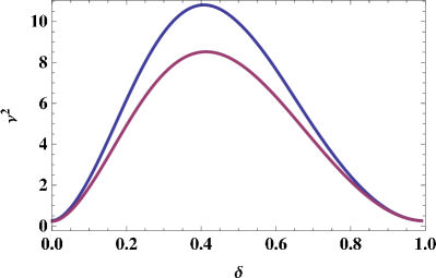
Let $x_{0}=x_{0}(c)$ be the solution of this equation. As shown in Fig. 1, the function $x_{0}(c)$ is the multiple valued function of $c$ and

$$x_{0}=x_{0n}(c),\qquad x_{0n}(1)=n\,\pi,\qquad n=1,2,3,\cdots.$$ (23)

Figure 1: The function $x_{0}(c)$. Each line corresponds to $x_{01},x_{02},x_{03}$.

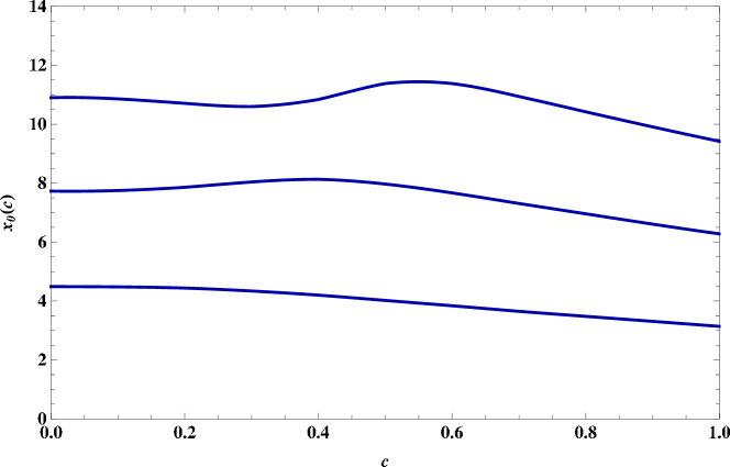
To make the commutation relation vanish at $r\neq 0$, the distance $r$ must satisfy the following equation

$$k_{c}r=x_{0}\left(\frac{k_{0}}{k_{c}}\right),\qquad k_{0}\leq k_{c}.$$ (24)

Conversely, for any given two points with $r\neq 0$, this relation provides the scale of the coarse graining $k_{0}/k_{c}$ which defines the bipartite system for the variable (21). In other words, if we specify the distance between spatially separated two points, at which we want to observe the quantum correlation between them, the scale of the coarse graining of the scalar field is determined by the relation (24). If this condition is satisfied, a measurement of the scalar field as the bipartite system becomes possible. We rewrite Eq. (24) as

$$k_{0}r=\delta\,x_{0}(\delta)$$ (25)

where

$$\delta\equiv\frac{k_{0}}{k_{c}},\qquad 0\leq\delta\leq 1$$

determines the scale of the coarse-graining. For $\delta=1~{}(k_{c}=k_{0})$, the distance is maximum

$$k_{0}r_{\text{max}}=x_{0}(1)=n\pi.$$ (26)

As the value $r_{\text{max}}$ corresponds to the system size related to the infrared cutoff $k_{0}$, we must set $n=1$. Hereafter, we adopt the smallest branch $x_{01}$ as the function $x_{0}(c)$.

The correlation functions of the scalar field are given by

$$c_{1}\equiv\frac{1}{2}\langle\hat{\varphi}(\boldsymbol{x}_{1})\hat{\varphi}(\boldsymbol{x}_{2})+\hat{\varphi}(\boldsymbol{x}_{2})\hat{\varphi}(\boldsymbol{x}_{1})\rangle=\frac{W_{0}^{2}}{2\pi^{2}}\int_{k_{0}}^{k_{c}}\!\!\!dkk^{2}\left(\frac{\sin kr}{kr}\right)|f_{k}|^{2},$$

$$c_{2}\equiv\frac{1}{2}\langle\hat{p}(\boldsymbol{x}_{1})\hat{p}(\boldsymbol{x}_{2})+\hat{p}(\boldsymbol{x}_{2})\hat{p}(\boldsymbol{x}_{1})\rangle=\frac{W_{0}^{2}}{2\pi^{2}}\int_{k_{0}}^{k_{c}}\!\!\!dkk^{2}\left(\frac{\sin kr}{kr}\right)|g_{k}|^{2},$$ (27)

$$c_{3}\equiv\frac{1}{2}\langle\hat{\varphi}(\boldsymbol{x}_{1})\hat{p}(\boldsymbol{x}_{2})+\hat{p}(\boldsymbol{x}_{2})\hat{\varphi}(\boldsymbol{x}_{1})\rangle=\frac{W_{0}^{2}}{2\pi^{2}}\int_{k_{0}}^{k_{c}}\!\!\!dkk^{2}\left(\frac{\sin kr}{kr}\right)\frac{i}{2}(f_{k}g_{k}^{*}-f_{k}^{*}g_{k}),$$

$$a_{1}=c_{1}(r=0),\quad a_{2}=c_{2}(r=0),\quad a_{3}=c_{3}(r=0).$$

By changing the integral variable to $z=k/k_{c}$, we have

$$c_{1}=\frac{3}{1-\delta^{3}}\int_{\delta}^{1}\!\!\!dzz^{2}j_{0}(x_{0}(\delta)z)|f_{k}(\eta)|_{k=k_{0}z/\delta}^{2},$$

$$c_{2}=\frac{3}{1-\delta^{3}}\int_{\delta}^{1}\!\!\!dzz^{2}j_{0}(x_{0}(\delta)z)|g_{k}(\eta)|_{k=k_{0}z/\delta}^{2},$$ (28)

$$c_{3}=\frac{3}{1-\delta^{3}}\int_{\delta}^{1}\!\!\!dzz^{2}j_{0}(x_{0}(\delta)z)\frac{i}{2}(f_{k}(\eta)g_{k}^{*}(\eta)-f_{k}^{*}(\eta)g_{k}(\eta))|_{k=k_{0}z/\delta}.$$

They are components of the $4\times 4$ covariance matrix (4)

$$\boldsymbol{V}=\begin{pmatrix}\boldsymbol{A}&\boldsymbol{C}\\ \boldsymbol{C}&\boldsymbol{A}\end{pmatrix},\quad\boldsymbol{A}=\begin{pmatrix}a_{1}&a_{3}\\ a_{3}&a_{2}\end{pmatrix},\quad\boldsymbol{C}=\begin{pmatrix}c_{1}&c_{3}\\ c_{3}&c_{2}\end{pmatrix}.$$

Using these components of the covariance matrix $\boldsymbol{V}$, the symplectic eigenvalues are expressed as

$$(\nu_{-})^{2}=a_{1}a_{2}-a_{3}^{2}+c_{1}c_{2}-c_{3}^{2}-|a_{1}c_{2}+a_{2}c_{1}-2a_{3}c_{3}|,$$ (29)

$$(\tilde{\nu}_{-})^{2}=a_{1}a_{2}-a_{3}^{2}-c_{1}c_{2}+c_{3}^{2}-|(a_{1}c_{2}-a_{2}c_{1})^{2}+4(a_{1}c_{3}-a_{3}c_{1})(a_{2}c_{3}-a_{3}c_{2})|^{1/2}.$$ (30)

III Entanglement of the quantum field in the Minkowski spacetime

As an application of our formalism, we first investigate the entanglement of the massive scalar field in the Minkowski spacetime. The mode function for the vacuum state in the Minkowski spacetime is

$$f_{k}=\frac{1}{\sqrt{2\omega}}\,e^{-i\omega t},\qquad g_{k}=i\sqrt{\frac{\omega}{2}}\,e^{-i\omega t},\qquad\omega=\sqrt{k^{2}+m^{2}}.$$ (31)

The correlation functions are

$$c_{1}=\frac{3}{2k_{0}}\frac{\delta}{1-\delta^{3}}\int_{\delta}^{1}dzz^{2}j_{0}(x_{0}(\delta)z)\left(z^{2}+\frac{m^{2}\delta^{2}}{k_{0}^{2}}\right)^{-1/2},$$

$$c_{2}=\frac{3k_{0}}{2}\frac{1}{\delta(1-\delta^{3})}\int_{\delta}^{1}dzz^{2}j_{0}(x_{0}(\delta)z)\left(z^{2}+\frac{m^{2}\delta^{2}}{k_{0}^{2}}\right)^{1/2},$$

$$c_{3}=0.$$

The relation between the distance $r$ and the logarithmic negativity is shown in Fig. 2.

Figure 2: The relation between the spatial distance $r$ and the logarithmic negativity $E_{N}$ [log plot of $E_{N}(r)$]. Each line corresponds to the different value of the mass $m/k_{0}=0~{}\text{(blue, the upper line)},10~{}\text{(red)},20~{}\text{(yellow)},40~{}\text{(green, the lower line)}$. The inset is the same plot in the small $r$ region and shows exponential decay of $E_{N}$. The decay rate depends on the mass $m$ in the small $r$ region.

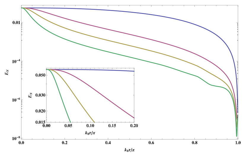
For any value of $m$, as the distance increases, the logarithmic negativity monotonically decreases but does not become zero. This implies that the Minkowski vacuum is always entangled. For $r\lesssim r_{c}\equiv 1/m$, we observe that $r$ dependence of $E_{N}$ is given by

$$E_{N}\sim e^{-r/r_{c}}$$ (32)

and the exponential decay rate is proportional to the mass $m$ (see the inset of Fig. 2). The entanglement concentrates in the region with the size of the Compton wavelength $\sim 1/m$. For $r_{c}\lesssim r\ll 1$, the decay law is

$$E_{N}\sim e^{-r/r_{0}}$$ (33)

where $r_{0}$ is a constant independent of mass $m$. In this region, the decay rate of the entanglement is the same for different values of $m$ including the massless case.

IV Entanglement of the quantum field in the expanding universe

We investigate the effect of the expansion rate of the Universe and the scalar field mass on the entanglement of the coarse-grained scalar field. We assume the following power law expansion of the Universe

$$a(t)=\left(1+\frac{H_{0}t}{p}\right)^{p},\qquad p>1,\quad H_{0}>0.$$ (34)

The conformal time is given by

$$\eta=\int_{0}^{t}\frac{dt}{a}=\frac{1}{H_{0}}\frac{p}{1-p}\left[\left(1+\frac{H_{0}t}{p}\right)^{1-p}-1\right],$$ (35)

and in terms of the conformal time, the scale factor is

$$a(\eta)=\left(\frac{\eta}{\eta_{0}}+1\right)^{\frac{p}{1-p}},\quad\eta_{0}=\frac{1}{H_{0}}\frac{p}{1-p}.$$ (36)

For the accelerated expansion $p>1$, we have $-\infty<\eta<-\eta_{0}$ and in the limit of $p\rightarrow\infty$,

$$\lim_{p\rightarrow\infty}a=\frac{1}{1-H_{0}\eta}=\exp(H_{0}t).$$

We set the initial time and the initial scale factor as $t=\eta=0$ and $a_{0}=1$.

We choose the cutoff parameter for the coarse graining of the scalar field as follows

$$k_{c}=\pi\epsilon aH=\pi\epsilon H_{0}\left(1+\frac{\eta}{\eta_{0}}\right)^{-1},\qquad k_{0}=\pi H_{0}.$$ (37)

At the initial time $t=\eta=0$, we prepare the spatial region with the size $H_{0}^{-1}$ and investigate how the entanglement of the scalar field between the spatially separated regions evolves as the Universe expands. We introduce the parameter $\epsilon$ to specify the scale of coarse graining and this parametrization is conventionally used for the stochastic approach to inflation StarobinskiA:1986 . In our analysis, this parameter must satisfy

$$\frac{H_{0}}{a\,H}\leq\epsilon$$ (38)

which comes from $k_{0}\leq k_{c}$. The value $\epsilon$ need not be smaller than unity that is usually assumed for the stochastic approach to inflation. We calculate the symplectic eigenvalue $\tilde{\nu}_{-}$ as a function of the physical distance

$$r_{\text{phys}}=ar=\frac{1}{\pi\epsilon H}x_{0}\left(\frac{H_{0}}{\epsilon aH}\right)$$ (39)

and the e-folding $N=\ln(a/a_{0})$. What we are interested in is the condition of the separability (8) and the classicality (10). We plot these conditions in the $(r_{\text{phys}},N)$ space.

IV.1 The effect of expansion rate on the entanglement

We first investigate the effect of the expansion rate of the Universe on the entanglement of the massless scalar field. In our previous paper NambuY:PRD78:2008 , we used a lattice model of the massless scalar field and found that the bipartite system becomes separable when the size of the spatial region exceeds the Hubble horizon. We aim to confirm this behavior for the accelerated universe with the power law expansion. The mode equation for the massless field is

$$f_{k}^{\prime\prime}+\left(k^{2}-\frac{\alpha^{2}-1/4}{(\eta+\eta_{0})^{2}}\right)f_{k}=0,\qquad\alpha^{2}=\frac{1}{4}\left(\frac{3p-1}{p-1}\right)^{2},$$ (40)

$$g_{k}=i\left(f_{k}^{\prime}-\frac{p}{1-p}\frac{f_{k}}{\eta+\eta_{0}}\right)$$

As the quantum state of the scalar field, we choose the Bunch-Davis vacuum state, the mode function is given by

$$f_{k}=\frac{\sqrt{\pi}}{2}e^{i(2\alpha+1)\pi/4}(-(\eta+\eta_{0}))^{1/2}H_{\alpha}^{(1)}(-k(\eta+\eta_{0})),$$ (41)

$$g_{k}=-i\frac{\sqrt{\pi}}{2}e^{i(2\alpha+1)\pi/4}k(-(\eta+\eta_{0}))^{1/2}H_{\alpha-1}^{(1)}(-k(\eta+\eta_{0})).$$ (42)

We first present the spatial dependence of the logarithmic negativity $E_{N}$ at the e-folding $N=10$ for the power index $p=100,10,5,3$ (Fig. 3). $E_{N}$ decays as $r_{\text{phys}}$ increases and becomes zero at $r_{\text{phys}}=r_{\text{separable}}$. For large spatial separation $r_{\text{separable}}<r_{\text{phys}}$, $E_{N}=0$ and the system is separable. We numerically check that the $p$ dependence of $r_{\text{separable}}$ is given by

$$r_{\text{separable}}\approx H_{0}^{-1}\exp\left(\frac{N}{p}\right)=H^{-1}.$$ (43)

Figure 3: Spatial dependence of the logarithmic negativity at $N=10$ for the massless field. The distance $r_{\text{phys}}$ is in the unit of $H_{0}^{-1}$. $E_{N}$ goes to zero at $r_{\text{phys}}=r_{\text{separable}}$. Each line corresponds to $p=100~{}\text{(blue, the lower line)},10~{}\text{(red)},5~{}\text{(yellow)},3~{}\text{(green, the upper line)}$.

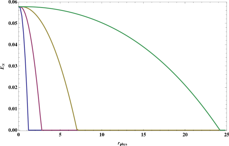
Hence, the horizon scale gives the scale of the separability and this result is consistent with our previous analysis using a lattice model NambuY:PRD78:2008 .

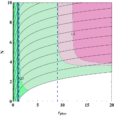
In Fig. 4, we show the behavior of the symplectic eigenvalue $(\tilde{\nu}_{-})^{2}$ in the $(r_{\text{phys}},N)$ space for the power index $p=100,10,5,3$. For the Universe with the power law expansion, the horizon scale $H^{-1}$ changes with time. We observe that the line of the separability condition $(\tilde{\nu}_{-})^{2}=1/4$ asymptotically coincides with the horizon line (the blue solid line). When the distance between two points is smaller than the horizon $H^{-1}$, they are entangled and they become disentangled after their separation exceeds the horion length.

Figure 4: The value of the symplectic eigenvalue $(\tilde{\nu}_{-})^{2}$ in the $(r_{\text{phys}},N)$ space for the massless scalar field in the Universe with power law expansion. The distance $r_{\text{phys}}$ is in the unit of $H_{0}^{-1}$. Each panel corresponds to the different expansion rate $p=100,10,5,3$ from the top left to the down right. The dark green region corresponds to $(\tilde{\nu}_{-})^{2}<1/4$ and the system is entangled in this region. The light green region corresponds to $1/4<(\tilde{\nu}_{-})^{2}<1$ and the system is separable but the classicality condition is not satisfied. The pink region corresponds to $1<(\tilde{\nu}_{-})^{2}$. The blue solid line is $r_{\text{phys}}=H^{-1}$ (horizon scale) and the black solid lines represent different comoving scales.

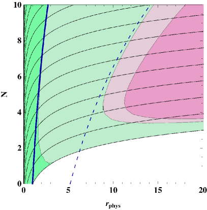
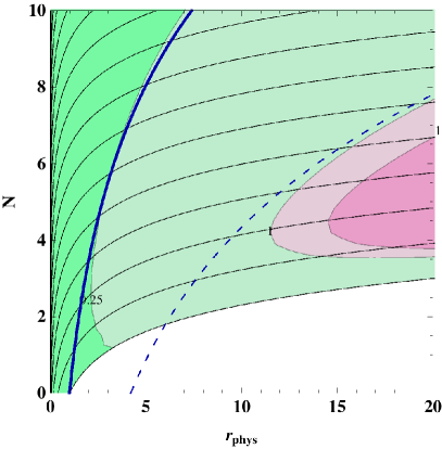
This behavior of disentanglement does not depend on the expansion rate $p$ and the condition of the separability is determined by $r_{\text{phys}}\approx H^{-1}$. Thus, for any value of $p>1$, for sufficiently large value of e-folding, the boundary between separable and entangled region coincides with the horizon line $H^{-1}$. This means the accelerated expansion of the Universe or the existence of the horizon determines the property of the separability of the massless scalar field in the expanding universe.

The line $(\tilde{\nu}_{-})^{2}=1$ giving the criterion of classicality asymptotically approaches several times larger than the horizon scale. In the region $(\tilde{\nu}_{-})^{2}>1$, the noncommutativity between canonical variables can be neglected when we evaluate the expectation values of operators and be consistent with the result obtained in the previous analysis for the behavior of the each comoving wave modeGuthAH:PRD32:1985 ; AlbrechtA:PRD50:1994 ; PolarskiD:CQG13:1996 ; LesgourguesJ:NPB497:1997 ; KieferC:CQG15:1998 ; for superhorizon scale quantum fluctuations, the noncommutativity between canonical variables becomes negligible because the growing mode solution is dominant and we can neglect $\hbar$ in the uncertainty relation. We confirmed the equivalent condition for the classicality from the condition of the existence of the classical distribution function and the symplectic eigenvalues.

IV.2 The effect of the mass on the entanglement

We next investigate the effect of the mass of the scalar field on the entanglement. For the massive scalar field in the de Sitter spacetime ($p=\infty$), the mode equation becomes

$$f_{k}^{\prime\prime}+\left(k^{2}-\frac{\alpha^{2}-1/4}{(\eta+\eta_{0})^{2}}\right)f_{k}=0,\qquad\alpha^{2}=\frac{9}{4}-\frac{m^{2}}{H_{0}^{2}},$$ (44)

$$g_{k}=i\left(f_{k}^{\prime}+\frac{f_{k}}{\eta+\eta_{0}}\right),\qquad\eta_{0}=-\frac{1}{H_{0}}$$

Assuming the Bunch-Davis vacuum state, the mode function is given by

$$f_{k}=\frac{\sqrt{\pi}}{2}e^{i(2\alpha+1)\pi/4}(-(\eta+\eta_{0}))^{1/2}H_{\alpha}^{(1)}(-k(\eta+\eta_{0})),$$ (45)

$$g_{k}=i\frac{\sqrt{\pi}}{2}e^{i(2\alpha+1)\pi/4}(-(\eta+\eta_{0}))^{-1/2}$$ (46)

$$\qquad\times\left[\left(\alpha-\frac{3}{2}\right)H_{\alpha}^{(1)}(-k(\eta+\eta_{0}))+k(\eta+\eta_{0})H_{\alpha-1}^{(1)}(-k(\eta+\eta_{0}))\right].$$

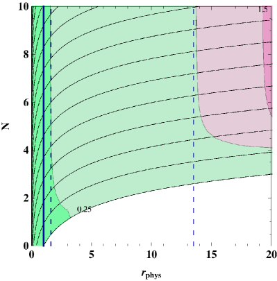
Fig. 5 shows the spatial dependence of $E_{N}$ at $N=10$ for $m^{2}/H_{0}^{2}=0,1/4,1/2,1$. $E_{N}$ decays as $r_{\text{phys}}$ increases and becomes zero at $r_{\text{phys}}=r_{\text{separable}}$. For large spatial separation $r_{\text{separable}}<r_{\text{phys}}$, $E_{N}=0$. We observe that the mass dependence of $r_{\text{separable}}$ is given by

$$r_{\text{separable}}\approx H_{0}^{-1}\left(1-c_{0}\,\frac{m^{2}}{2H^{2}}\right)^{-1/2},\qquad c_{0}\sim 1.4.$$ (47)

Figure 5: Spatial dependence of the logarithmic negativity at $N=10$ for the massive scalar field in the de Sitter spacetime. The distance $r_{\text{phys}}$ is in the unit of $H_{0}^{-1}$. Each line corresponds to $m^{2}/H_{0}^{2}=0~{}\text{(blue, the lower line)},1/4~{}\text{(red)},1/2~{}\text{(yellow)},3/4~{}\text{(green)},1~{}\text{(blue, the upper line)}$.

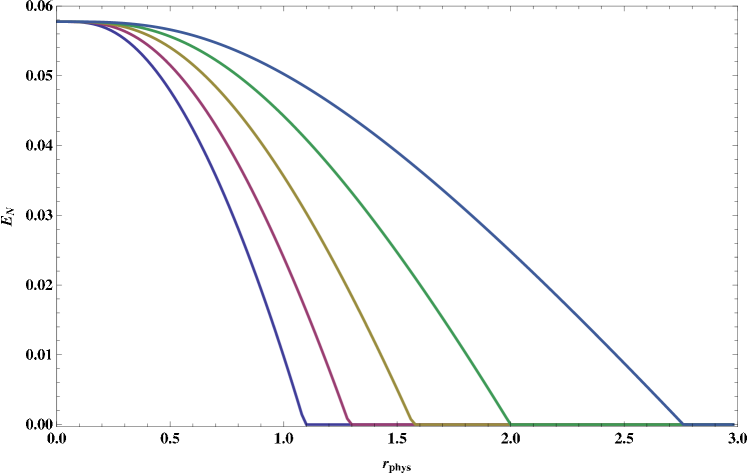
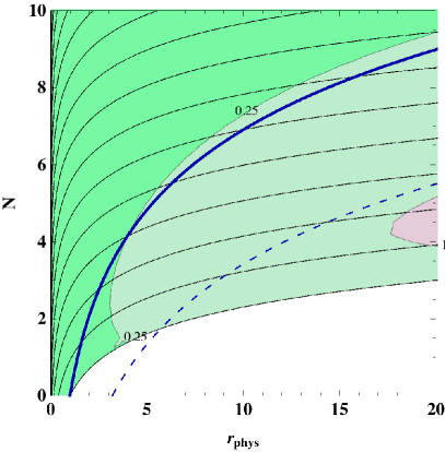
For $m\neq 0$, $r_{\text{separable}}$ does not coincide with the horizon scale $H_{0}^{-1}$, which is the characteristic scale of the disentanglement for the massless scalar field. The mass dependence (47) of $r_{\text{separable}}$ can be understood as follows. Let us recall the form of the mode equation (18). The mode changes its behavior depending on the following wave numbers:

$$\left(\frac{k_{*}}{a}\right)^{2}\equiv\frac{a^{\prime\prime}}{a^{3}}-m^{2}.$$ (48)

For $k>k_{*}$, the mode behaves oscillatory and for $k<k_{*}$, the mode becomes unstable and frozen. This critical wave number corresponds to the physical length

$$r_{*}=\frac{1}{H_{0}}\left(1-\frac{m^{2}}{2H_{0}^{2}}\right)^{-1/2}.$$ (49)

If the physical wavelength of the scalar field is smaller than this length, the scalar field behaves oscillatory and then becomes frozen after its wavelength exceeds $r_{*}$ by the cosmic expansion. For the massless case, $r_{*}$ coincides with the horizon length $H^{-1}$ and the nonzero mass increases the length $r_{*}$. Our numerical result (47) indicates

$$r_{\text{separable}}\approx r_{*}.$$ (50)

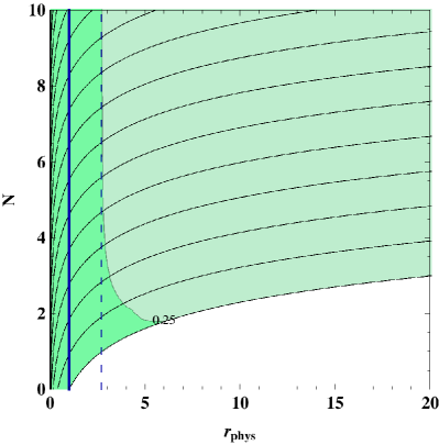
Figure 6 shows the $(r_{\text{phys}},N)$ dependence of the symplectic eigenvalue $(\tilde{\nu}_{-})^{2}$. For the massless case, for the sufficiently large value of the e-folding, the system becomes separable after the physical distance between two points exceeds the horizon $H_{0}^{-1}$. As the mass increases, the line $(\tilde{\nu}_{-})^{2}=1/4$ representing the separability condition deviates from the horizon line $H_{0}^{-1}$ as expected from (50). The line $\tilde{\nu}_{-}=1$, which gives the criterion of the classicality (10), corresponds to the scale $6\sim 7$ times larger than the horizon size.

We compare this behavior of the mass dependence on the entanglement with the Minkowski case. For the Minkowski spacetime, the characteristic size of the entangled region is given by the Compton wavelength $1/m$ and this size decreases as the mass increases. For the de Sitter case, if we consider a sufficiently small region compared to the horizon length, we can neglect the effect of the cosmic expansion and the behavior of the entanglement is the same as the Minkowski case. For larger scales $r_{*}<r_{\text{phys}}$, the system becomes separable and this disentanglement behavior does not occur in the Minkowski spacetime. The size of the entangled region is larger than the horizon scale and increases as the mass increases. We expect that this behavior of the entanglement is related to the causal structure of the de Sitter spacetime.

Figure 6: The $(r_{\text{phys}},N)$ dependence of the symplectic eigenvalue $(\tilde{\nu}_{-})^{2}$ for the massive scalar field in the de Sitter spacetime. The distance $r_{\text{phys}}$ is in units of $H_{0}^{-1}$. Each panel show $(\tilde{\nu}_{-})^{2}$ for $m^{2}/H_{0}^{2}=0,1/4,1/2,1$ from the top left to the down right. The dark green region corresponds to $(\tilde{\nu}_{-})^{2}<1/4$ and the system is entangled. The light green region corresponds to $(\tilde{\nu}_{-})^{2}>1/4$ and the system is separable. The pink region satisfies the condition of the classicality $(\tilde{\nu}_{-})^{2}>1$. The black solid lines represent the different comoving scales. The line $(\tilde{\nu}_{-})^{2}=1/4$ deviates from the horizon scale $H_{0}^{-1}$ (the blue solid line) as the mass increases.

IV.3 Classicality condition and scale of coarse graining

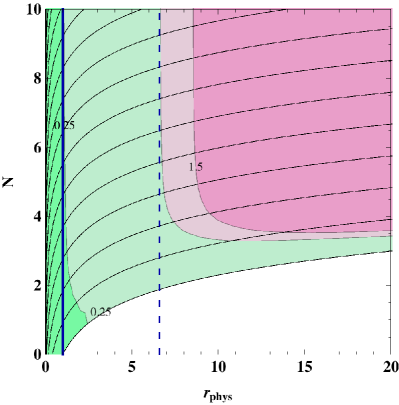
In this subsection, we discuss the relation between the classicality and the scale of coarse graining. As we have already observed, the coarse graining with a sufficiently large scale leads to $\tilde{\nu}_{-}\gg 1/4$ and the system becomes classical. To investigate the effect of the scale of coarse-graining on the classicality, we plot the symplectic eigenvalues as the function of $\delta=k_{0}/k_{c}$ in Fig. 7:

Figure 7: The dependence of the comoving scale $\delta$ of the symplectic eigenvalues for the massive scalar field in the de Sitter universe. The left panel shows $(\nu_{-})^{2}$ (blue line) and $(\tilde{\nu}_{-})^{2}$ (red line) at $N=2$. The right panel is at $N=5$. The mass of the scalar field is $m^{2}/H_{0}^{2}=1/4$. At any time, $\tilde{\nu}_{-}>1/2$ for $1/a<\delta\leq 1$.

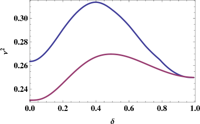
The relation between $\delta$ and the coarse-graining parameter $\epsilon$ is

$$\delta=\frac{H_{0}}{\epsilon\,a\,H}\leq 1.$$ (51)

As the physical distance is

$$ar=\frac{1}{\pi\epsilon H}x_{0}\left(\frac{H_{0}}{\epsilon aH}\right)\sim\frac{1}{\epsilon H},$$ (52)

$\delta$ represents the comoving scale of the bipartite system. For the super horizon scale $H_{0}/(aH)<\delta\leq 1$, as we have already confirmed, the separability condition $(\tilde{\nu})^{2}>1/4$ is satisfied. For late time $a\gg 1$, the classicality condition $(\tilde{\nu})^{2}\gg 1/4$ is also satisfied for a wide range of the comoving scale $\delta$. However, as is shown in the right panel of Fig. 7, for too large a value of $\delta$, the classicality condition is not satisfied as $\nu,\tilde{\nu}$ are decreasing functions of $\delta$ for $\delta\sim 1$. Thus, we have the maximum scale of the coarse graining to retain the classicality. We can estimate this scale using the asymptotic form of the correlation functions  (28) and the definition of the symplectic eigenvalue (30). Assuming the large scale coarse graining $\epsilon\ll 1$, we obtain the following asymptotic form of the symplectic eigenvalue $\nu$ and $\tilde{\nu}$ for the massive scalar field in the de Sitter spacetime:

$$\nu^{2},\tilde{\nu}^{2}\sim\begin{cases}&(a\,\delta)^{4\alpha-4}=\left(\dfrac{1}{\epsilon}\right)^{2}\qquad(\text{ for}~{}\delta\sim 0),\\ &a^{4\alpha-4}(1-\delta)^{2}+1/4=\epsilon^{4m^{2}/(3H_{0}^{2})}\left(a-\dfrac{1}{\epsilon}\right)^{2}+1/4\qquad(\text{ for}~{}\delta\sim 1)\end{cases}$$ (53)

where we have used $\alpha\approx 3/2-m^{2}/(3H_{0}^{2}),~{}m^{2}/H_{0}^{2}\ll 1$. For the small comoving scale $\delta\sim 0$, the classicality condition $\tilde{\nu}^{2}\gg 1/4$ requires $\epsilon\ll 1$ and this is consistent with $\delta\sim 0$ provided that $a\gg 1$ (late time). Thus, sufficiently large scale coarse graining $\epsilon\ll 1$ is necessary to obtain the classicality of the scalar field. For the large comoving scale $\delta\sim 1$, to keep $\tilde{\nu}^{2}\gg 1/4$,

$$1\ll\epsilon^{2m^{2}/(3H_{0}^{2})}=e^{2m^{2}/(3H_{0}^{2})\ln\epsilon}$$ (54)

is necessary and this yields the lower bound of $\epsilon$:

$$e^{-3H_{0}^{2}/(2m^{2})}\ll\epsilon.$$ (55)

Therefore, we need the following condition for the coarse-graining parameter to guarantee the classicality of the coarse-grained field

$$e^{-3H_{0}^{2}/(2m^{2})}\ll\epsilon\ll 1.$$ (56)

For the massless scalar field in the Universe with a power law expansion, we have

$$\nu^{2},\tilde{\nu}^{2}\sim\begin{cases}&\left(\dfrac{a\,\delta\,H}{H_{0}}\right)^{4\alpha-4}=\left(\dfrac{1}{\epsilon}\right)^{2}\qquad(\text{ for}~{}\delta\sim 0),\\ &\left(\dfrac{aH}{H_{0}}\right)^{4\alpha-4}(1-\delta)^{2}+1/4=\epsilon^{-4/p}\left(\dfrac{aH}{H_{0}}-\dfrac{1}{\epsilon}\right)^{2}+1/4\qquad(\text{ for}~{}\delta\sim 1)\end{cases}$$ (57)

where we have used $\alpha\approx 3/2+1/p,~{}p\gg 1$. The condition $\tilde{\nu}^{2}\gg 1/4$ leads to

$$\epsilon\ll 1.$$ (58)

The condition (56) and (58) for the coarse-graining parameter $\epsilon$ are the same as the ones that appeared in the stochastic approach to inflation StarobinskiA:1986 ; SasakiM:NPB308:1988 ; HabibS:PRD46:1992 to ensure the amplitude of the stochastic noise is independent of the coarse-graining parameter. With these conditions, the stochastic calculus based on the Langevin equation reproduces the field theoretic result of expectation values. However, in the context of the stochastic approach, it was not clear why these conditions guarantee the validity of the stochastic approach. From the view point of the entanglement and the classicality of the quantum field, the conditions (56) and (58) are equivalent to $\tilde{\nu}^{2}\gg 1/4$; with this condition, the coarse-grained quantum field becomes separable and there exists a classical distribution function which reproduces the expectation values of the original quantum system. In other words, we have appropriate classical stochastic variables or stochastic processes that mimic the original quantum dynamics. This supports the validity of the stochastic approach which treats the quantum field as the classical stochastic variables.

V Summary and conclusion

We investigated the behavior of the bipartite entanglement of the scalar field in the expanding universe. To define the bipartite system for the quantum field, we introduced the coarse graining of the scalar field. In our formalism, the scale of the coarse graining corresponds to the spatial distance between two points at which we want to measure the bipartite entanglement. This defines the bipartite system with the two mode Gaussian state and we can judge the separability of the system by the criterion based on the partial transpose operation.

For the massless field, the disentanglement occurs when the scale of the coarse graining equals to the horizon length $H^{-1}$. The horizon scale determines the causal structure of the accelerated expanding universe and two points are causally disconnected beyond this scale. We have confirmed that the quantum correlation or the bipartite entanglement disappears beyond this scale for the massless scalar field. This disentanglement behavior is necessary for the quantum field to acquire the classical nature. With inclusion of the mass of the scalar field, we found that the mass increases the scale of the disentanglement. The system becomes separable when the oscillatory behavior of the mode function stops and changes to be frozen. This scale is larger than the horizon length and corresponds to the sonic horizon which discriminates the behavior of the mode function. After the disentanglement occurs and the system becomes separable, the classicality condition is satisfied at a sufficiently late time or for sufficiently large scale coarse graining. We derived the condition for the scale of the coarse graining needed to satisfy the classicality condition at late time and found that the upper and the lower bound for the coarse-graining parameter. These bounds are equivalent to ones that appeared in the stochastic approach to inflation to guarantee the cut-off independence of the stochastic dynamics of the scalar field.

After the classicality condition is satisfied, it is possible to calculate the quantum expectation value of any operators using the classical distribution functions such as the $P$ function and the Wigner function. However, this does not mean that the information on the quantum correlation or the entanglement before the classicalization is lost. The remnant of the quantum correlation is encoded in the classical distribution function and this is responsible for the origin of structure in our Universe. It will be interesting to investigate the relation between the classical stochastic property of the fluctuation after the classicalization and the encoded quantum correlation. The analysis towards such a direction will make clear the mechanism of the quantum to classical transition of the quantum fluctuation in the inflationary universe.