SET: AN ALGORITHM FOR CONSISTENT MATRIX COMPLETION

Abstract

A new algorithm, termed subspace evolution and transfer (SET), is proposed for solving the consistent matrix completion problem. In this setting, one is given a subset of the entries of a low-rank matrix, and asked to find one low-rank matrix consistent with the given observations. We show that this problem can be solved by searching for a column space that matches the observations. The corresponding algorithm consists of two parts — subspace evolution and subspace transfer. In the evolution part, we use a line search procedure to refine the column space. However, line search is not guaranteed to converge, as there may exist barriers along the search path that prevent the algorithm from reaching a global optimum. To address this problem, in the transfer part, we design mechanisms to detect barriers and transfer the estimated column space from one side of the barrier to the another. The SET algorithm exhibits excellent empirical performance for very low-rank matrices.

I Introduction

Suppose that we observe a subset of entries of a matrix. The matrix completion problem asks when and how the matrix can be uniquely recovered based on the observed entries. This reconstruction task is ill-posed and computationally intractable. However, if the data matrix is known to have low-rank, exact recovery can be accomplished in efficient manners, provided that sufficiently many entries are revealed. Low-rank matrix completion problem has received considerable interests due to its wide applications, see for example [5] for more details.

An efficient way to solve the completion problem is via convex relaxation. Instead of looking at rank-restricted matrices, one can search for the matrix with minimum nuclear norm, subject to data consistency constraints. Although in general nuclear norm minimization is not equivalent to rank minimization, the former approach recovers the same solution as the latter if the data matrix satisfies certain incoherence conditions [6]. More importantly, nuclear norm minimization can be accomplished by polynomial complexity algorithms, for example, semi-definite programming or singular value thresholding (SVT) [1].

There are other low-complexity alternatives. Based on the subspace pursuit (SP) and CoSaMP algorithms for compressive sensing [7, 8], the authors of [2] developed the so called ADMiRA algorithm. A modification of the power factorization algorithm was used for matrix completion in [3]. Another approach for solving this problem, termed OptSpace, was described in [4].

The problem considered in this paper and its algorithmic solution differ from all previously published approaches. The problem at hand is to identify one low-rank matrix consistent with the observations. The solution may or may not be unique. In contrast, most results in matrix completion deal with the somewhat more restrictive requirement that the reconstruction is unique. Hence, our approach can be applied to scenarios where the matrix is highly under-sampled, and where potentially many consistent solutions exist. The relaxation on uniqueness allows for the empirically observed performance improvement over other completion techniques.

To solve the consistent matrix completion problem, we propose an algorithm, termed subspace evolution and transfer (SET). We show that the matrix completion problem can be solved by searching for a column (or row) space that matches the observations. As a result, optimization on the Grassmann manifold, i.e., subspace evolution, plays a central role in the algorithm. However, there may exist “barriers” along the search path that prevent subspace evolution from converging to a global optimum. To address this problem, in the subspace transfer part, we design mechanisms to detect and cross barriers. Empirical simulations demonstrate the excellent performance of the proposed algorithm.

Despite resembling the OptSpace algorithm [4] in terms of using optimization over Grassmann manifolds, our approach substantially differs from this algorithm. Searching over only one space (column or row space) represents one of the most significant differences: in OptSpace, one searches both column and row spaces simultaneously, which introduces numerical and analytical difficulties. Moreover, when optimizing over the column space, one has to take care of “barriers” that prevent the search procedure from converging to a global optimum, an issue that was not addressed before since it was obscured by simultaneous column and row space searches.

II Consistent Matrix Completion

Let $\bm{X}\in\mathbb{R}^{m\times n}$ be an unknown matrix with rank $r\ll\min\left(m,n\right)$, and let $\Omega\subset\left[m\right]\times\left[n\right]$ be the set of indices of the observed entries, where $\left[K\right]=\left\{1,2,\cdots,K\right\}$. Define the projection operator $\mathfrak{P}_{\Omega}:\;\mathbb{R}^{m\times n}\rightarrow\mathbb{R}^{m\times n}$ by

$$\bm{X} \mapsto\bm{X}_{\Omega},\;\mbox{where }\left(\bm{X}_{\Omega}\right)_{i,j}=\begin{cases}\bm{X}_{i,j}&\mbox{if }\left(i,j\right)\in\Omega\\ 0&\mbox{if }\left(i,j\right)\notin\Omega\end{cases}.$$

The consistent matrix completion problem is to find one rank-$r$ matrix $\bm{X}^{\prime}$ that is consistent with the observations $\bm{X}_{\Omega}$, i.e.,

$$\left(P0\right):\; \mbox{find }\bm{X}^{\prime}\mbox{ such that }$$

$$\mbox{rank}\left(\bm{X}^{\prime}\right)\leq r\mbox{ and }\mathfrak{P}_{\Omega}\left(\bm{X}^{\prime}\right)=\mathfrak{P}_{\Omega}\left(\bm{X}\right)=\bm{X}_{\Omega}.$$ (1)

This problem is well defined as $\bm{X}_{\Omega}$ is generated from the matrix $\bm{X}$ with rank $r$ and therefore there must exist at least one solution. In this paper, like in other approaches in [2, 3, 4], we assume that the rank $r$ is given. In practice, one may try to sequentially guess a rank bound until a satisfactory solution has been found.

III The SET Algorithm

III-A Why optimize over column spaces only?

In this section, we show that the problem $\left(P0\right)$ is equivalent to finding a column space consistent with the observations.

Let $\mathcal{U}_{m,r}$ be the set of $m\times r$ matrices with $r$ orthonormal columns, i.e., $\mathcal{U}_{m,r}=\left\{\bm{U}\in\mathbb{R}^{m\times r}:\;\bm{U}^{T}\bm{U}=\bm{I}_{r}\right\}.$ Define a function

$$f:\;\mathcal{U}_{m,r} \rightarrow\mathbb{R}$$

$$\bm{U} \mapsto\underset{\bm{W}\in\mathbb{R}^{n\times r}}{\min}\left\|\bm{X}_{\Omega}-\mathfrak{P}_{\Omega}\left(\bm{U}\bm{W}^{T}\right)\right\|_{F}^{2},$$ (2)

where $\left\|\cdot\right\|_{F}$ denotes the Frobenius norm. The function $f$ captures the consistency between the matrix $\bm{U}$ and the observations $\bm{X}_{\Omega}$: if $f\left(\bm{U}\right)=0$, then there exists a matrix $\bm{W}$ such that the rank-$r$ matrix $\bm{U}\bm{W}^{T}$ satisfies $\mathfrak{P}_{\Omega}\left(\bm{U}\bm{W}^{T}\right)=\bm{X}_{\Omega}$. Hence, the consistent matrix completion problem is equivalent to

$$\left(P1\right):\; \mbox{find }\bm{U}\in\mathcal{U}_{m,r}\;\mbox{such that }f\left(\bm{U}\right)=0.$$ (3)

The solution $f\left(\bm{U}\right)$ is not unique in the space $\mathcal{U}_{m,r}$. An important property of $f$ is that $f\left(\bm{U}\right)=f\left(\bm{U}\bm{V}\right)$ for any $r$-by-$r$ orthogonal matrix $\bm{V}$, since $\bm{U}\bm{W}^{T}=\left(\bm{U}\bm{V}\right)\left(\bm{W}\bm{V}\right)^{T}$. Hence, the function $f$ depends only on the subspace spanned by the columns of $\bm{U}$, i.e., the $\mbox{span}\left(\bm{U}\right)$. Note that all columns of the matrix of the form $\bm{U}\bm{W}^{T}$ lie in the linear subspace $\mbox{span}\left(\bm{U}\right)$. The consistent matrix completion problem is essentially finding a column space consistent with the observed entries.

We find the following definitions useful for the exposition to follow. The set of all $r$-dimensional linear subspaces in $\mathbb{R}^{n}$ is called the Grassmann manifold, and is denoted by $\mathcal{G}_{m,r}$. Given a subspace $\mathscr{U}\in\mathcal{G}_{m,r}$, one can always find a matrix $\bm{U}\in\mathcal{U}_{m,r}$, such that $\mathscr{U}=\mbox{span}\left(\bm{U}\right)$. The matrix $\bm{U}$ is referred to as a generator matrix of $\mathscr{U}$. Although a given subspace $\mathscr{U}\in\mathcal{G}_{m,r}$ has multiple generator matrices, a given matrix $\bm{U}\in\mathcal{U}_{m,r}$ uniquely defines a subspace. For this reason, we henceforth use $\bm{U}$ to represent its generated subspace.

III-B The SET algorithm: a high level description

Our algorithm aims to minimize the objective function $f\left(\bm{U}\right)$, provided that the minimum value of $f\left(\bm{U}\right)$ is known to be zero. Ideally, a solution can be obtained by using a line search procedure on the Grassmann manifold. Here, line search refers to iterative refinements of the interval in which the function attains its minimum. Hence, the “subspace evolution” part of the algorithm reduces to a well studied optimization method.

The main difficulty that arises during line search, and makes the SET algorithm highly non-trivial is when during the search, one encounters “barriers”. Careful inspection reveals that the objective function $f$ can be decomposed into a sum of atomic functions, each of which involves only one column of $\bm{X}_{\Omega}$ (see Section III-D for details). Along the gradient descent path, these atomic functions may not agree with each other: some decrease and some increase. Increases of some atomic functions may result in “bumps” in the $f$ curve, which block the search procedure from global optima and are therefore referred to as barriers. The main component of the “transfer” part of the algorithm is to identify whether there exist barriers along the gradient descent path. Detecting barriers is in general a very difficult task, since one does not know the locations of global minima. Nevertheless, we observe that barriers can be detected by the existence of atomic functions with inconsistent descent directions. When such a scenario is encountered, the algorithm “transfers” the starting point of line search to the other side of the barriers, and proceeds from there. Such a transfer does not overshoot global minima as we enforce consistency of the steep descent directions at the points before and after the transfer.

In summary, we start with a randomly generated $\bm{U}\in\mathcal{U}_{m,r}$ and then refine it until $f\left(\bm{U}\right)=0$. At each iteration, we first detect and then cross barriers if there are any, and then perform line search. The details of subspace evolution and transfer are given in Section III-C and III-D. Simulation results are presented in Section IV.

III-C Subspace evolution

Due to space limitation, we focus on the $r=1$ case in Sections III-C and III-D. Furthermore, our exposition aims to make the algorithmic details as transparent to the readers as possible. The highly technical performance and complexity analysis of SET for both $r=1$ and $r>1$ is deferred to the journal version of the paper.

For the optimization problem at hand, we shall refine the current column space estimate $\bm{u}$ following the gradient descent direction. Here, the lowercase letter $\bm{u}$ is used to emphasize that the $\bm{U}$ matrix is a vector when $r=1$. Let $\bm{w}_{\bm{u}}$ be a length-$n$ column vector that achieves $f\left(\bm{u}\right)$, and let $\bm{X}_{r}=\bm{X}_{\Omega}-\mathfrak{P}_{\Omega}\left(\bm{u}\bm{w}_{\bm{u}}^{T}\right)$. Then the gradient of $f$ at $\bm{u}$ is given by

$$\nabla_{\bm{u}}f =-2\bm{X}_{r}\bm{w}_{\bm{u}}.$$ (4)

The gradient descent path is chosen to be the geodesic curve on the Grassmann manifold with direction $\bm{h}=-\nabla_{\bm{u}}f/\left\|\nabla_{\bm{u}}f\right\|_{F}$. A geodesic surve is an analogue of a straight line in an Euclidean space: given two points on the manifold, the geodesic curve connecting them is the path of the shortest length on the manifold. According to [9, Theorem 2.3], the geodesic curve starting from $\bm{u}$, along $\bm{h}$, is given by

$$\bm{u}\left(t\right)=\bm{u}\cos t+\bm{h}\sin t,\quad t\in\left[0,\pi\right).$$ (5)

We restrict $t$ to the interval $\left[0,\pi\right)$ because $f\left(\bm{u}\left(t\right)\right)$ has period $\pi$, i.e., $f\left(\bm{u}\left(t+\pi\right)\right)=f\left(-\bm{u}\left(t\right)\right)=f\left(\bm{u}\left(t\right)\right)$. Interested readers are referred to [9] for more details on geodesics on the Grassmann manifold.

The subspace evolution part is designed to search for a minimizer (in most cases, a local minimizer) of the function $f$ along the geodesic curve. Our implementation includes two steps. The goal of the first step is to identify an interval $\left[0,t_{\max}\right]$ that contains a minimizer. Since $f\left(t\right)$ is periodic, $t_{\max}$ is upper bounded by $\pi$. The second step is devoted to locating the minimizer $t^{*}\in\left[0,t_{\max}\right]$ accurately by iteratively applying the golden section rule [10]. These two steps are described in Algorithm 1. The constants are set to $\epsilon=10^{-9}$, $c_{1}=\left(\sqrt{5}-1\right)/2$, $c_{2}=c_{1}/\left(1-c_{1}\right)$ and $itN=10$. Ideally, the starting step size $\epsilon>0$ should be chosen as small as possible. We fix it to a constant as computers only have finite precision and $10^{-9}$ is already sufficiently small in all our experiments.

Algorithm 1 Subspace evolution.

Input: $\bm{X}_{\Omega}$, $\Omega$, $\bm{u}$, and $itN$.

Output: $t^{*}$ and $\bm{u}\left(t^{*}\right)$.

Step A: find $t_{\max}\leq\pi$ such that $t^{*}\in\left[0,t_{\max}\right]$

Let $t^{\prime}=\epsilon\pi$.

1. Let $t^{\prime\prime}=c_{2}\cdot t^{\prime}$. If $t^{\prime\prime}>\pi$, then $t_{\max}=\pi$ and quit Step A.

2. If $f\left(\bm{u}\left(t^{\prime\prime}\right)\right)>f\left(\bm{u}\left(t\right)\right)$, then $t_{\max}=t^{\prime\prime}$ and quit Step A.

3. Otherwise, $t^{\prime}=t^{\prime\prime}$. Go back to step 1).

Step B: numerically search for $t^{*}$ in $\left[0,t_{\max}\right]$.

Let $t_{1}=t_{\max}/c_{2}^{2}$, $t_{2}=t_{\max}/c_{2}$, $t_{4}=t_{\max}$, and $t_{3}=t_{1}+c_{1}\left(t_{4}-t_{1}\right)$. Let $itn=1$. Perform the following iterations.

1. If $f\left(\bm{u}\left(t_{1}\right)\right)>f\left(\bm{u}\left(t_{2}\right)\right)>f\left(\bm{u}\left(t_{3}\right)\right)$, then $t_{1}=t_{2}$, $t_{2}=t_{3}$, and $t_{3}=t_{1}+c_{1}\left(t_{4}-t_{1}\right)$.

2. Else, $t_{4}=t_{3}$, $t_{3}=t_{2}$ and $t_{2}=t_{1}+\left(1-c_{1}\right)\left(t_{4}-t_{1}\right)$.

3. $itn=itn+1$. If $itn>itN$, then quit the iterations. Otherwise, go back to step 1).

Let $t^{*}=\underset{t\in\left\{t_{1},\cdots,t_{4}\right\}}{\arg\min}f\left(\bm{u}\left(t\right)\right)$ and compute $\bm{u}\left(t^{*}\right)$.

III-D Subspace transfer

Unfortunately, the objective function $f\left(\bm{u}\right)$ may not be a convex function of $\bm{u}$. The described linear search procedure may not converge to a global minimum because the search path may be blocked by what we call “barriers”. We show next how to overcome the problem introduced by barriers.

At this point, we formally introduce the decoupling principle: the objection function $f\left(\bm{u}\left(t\right)\right)$ is the squared Frobenius norm of the residue matrix; it can be decomposed as the sum of the squared Frobenius norm of the residue columns. More precisely, let $\bm{x}_{\Omega_{j}}\in\mathbb{R}^{m\times 1}$ be the $j^{th}$ column of the matrix $\bm{X}_{\Omega}$. Let $\mathfrak{P}_{\Omega_{j}}:\;\mathbb{R}^{m\times 1}\rightarrow\mathbb{R}^{m\times 1}$ be the projection operator corresponding to the $j^{th}$ column, defined by

$$\bm{v} \mapsto\bm{v}_{\Omega_{j}},\;\mbox{where}\;\left(\bm{v}_{\Omega_{j}}\right)_{i}=\begin{cases}\bm{v}_{i}&\mbox{if }\left(i,j\right)\in\Omega\\ 0&\mbox{if }\left(i,j\right)\notin\Omega\end{cases}.$$

Then the objective function $f\left(\bm{u}\left(t\right)\right)$ can be written as a sum of $n$ atomic functions:

$$f\left(\bm{u}\left(t\right)\right) =\underset{\bm{w}\in\mathbb{R}^{n\times 1}}{\min}\left\|\bm{X}_{\Omega}-\mathfrak{P}_{\Omega}\left(\bm{u}\bm{w}^{T}\right)\right\|_{F}^{2}$$

$$=\sum_{j=1}^{n}\underbrace{\min_{\bm{w}_{j}\in\mathbb{R}}\left\|\bm{x}_{\Omega_{j}}-\mathfrak{P}_{\Omega_{j}}\left(\bm{u}\left(t\right)\bm{w}_{j}\right)\right\|_{F}^{2}}_{f_{j}\left(\bm{u}\left(t\right)\right)}.$$ (6)

This principle is essential to understanding the behavior of $f\left(\bm{u}\left(t\right)\right)$.

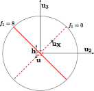
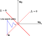
The following example illustrates the concept of a barrier. Consider an incomplete observation of a rank-one matrix $\left[\left[?,2,2\right]^{T},\left[2,?,1\right]^{T}\right],$ where question marks denote that the corresponding entries are unknown. It is clear that the objective function $f\left(\bm{u}\left(t\right)\right)$ is minimized by $\bm{u}_{\bm{X}}=\frac{1}{\sqrt{6}}\left[2,1,1\right]^{T}$, i.e., $f\left(\bm{u}_{\bm{X}}\right)=0$. Suppose that one starts with the initial guess $\bm{u}=\frac{1}{\sqrt{102}}\left[-10,1,1\right]^{T}$. The contours of the atomic function $f_{1}\left(\bm{u}\right)$, projected on the plane spanned by $\bm{u}_{2}$ and $\bm{u}_{3}$, is depicted in Fig. 1a. All $\bm{u}$’s with $\bm{u}_{2}=-\bm{u}_{3}$ lie on the contour $f_{1}\left(\bm{u}\right)=8$. Computations show that the gradient descent direction $\bm{h}$ is pointing upward. However $f\left(\bm{u}\right)=f_{1}\left(\bm{u}\right)+f_{2}\left(\bm{u}\right)=0+f_{2}\left(\bm{u}\right)\leq 5<8$. Any gradient descent algorithms can not pass through the contour $f_{1}\left(\bm{u}\right)=8$. Careful tracking of several line search steps (Fig. 1b) shows that $\bm{u}\left(t\right)$ will approach $\left[-1,0,0\right]^{T}$, but will never cross the contour $f_{1}=8$. That is, the contour $f_{1}=8$ forms a “barrier” for the line search procedure.

(a) Contours of $f_{1}$.

(b) Search paths with zooming in.

Figure 1: An illustrative example for barriers.

It is possible to detect barriers algorithmically. It can be verified that $f_{j}\left(\bm{u}\left(t\right)\right)$ has a unique minimizer and maximizer, given by

$$t_{\max,j}=\underset{t\in\left[0,\pi\right)}{\arg\max}f_{j}\left(\bm{u}\left(t\right)\right)\;\mbox{and}\;t_{\min,j}=\underset{t\in\left[0,\pi\right)}{\arg\min}f_{j}\left(\bm{u}\left(t\right)\right)$$ (7)

respectively. There are closed-form equations for these two quantities given an initial vector $\bm{u}$ and a direction $\bm{h}$. We say that the $k^{th}$ column of $\bm{X}_{\Omega}$ forms a barrier if there exists a $j\in\left[n\right]$, $j\neq k$, such that

1. the maximizer of $f_{k}$ appears before the minimizer of $f_{j}$, i.e., $t_{\max,k}<t_{\min,j}<t_{\max,j}$; and

2. the gradients of $f$ at $\bm{u}\left(0\right)$ and $\bm{u}\left(t_{\max,k}\right)$ are consistent (form a sharp angle), i.e., $\frac{d}{dt}f\left(\bm{u}\left(t\right)\right)|_{t=t_{\max,k}}<0$.

When a barrier is detected, we transfer $\bm{u}$ from one side of it to the other. In our implementation, we focus on the closest barriers to $\bm{u}$ to avoid overshooting. Define

$$\mathcal{J}=\left\{j:\;\mbox{the }j^{th}\mbox{ column of }\bm{X}_{\Omega}\;\mbox{admits barriers}\right\},$$

$$j^{*}=\underset{j\in\mathcal{J}}{\arg\min}\;t_{p,j},\;\mbox{and}$$ (8)

$$k^{*} =\underset{k}{\arg\max}\;\left\{t_{o,k}:\;\mbox{the }k^{th}\mbox{ column of }\bm{X}_{\Omega}\;\mbox{forms a barrier}\right.$$

$$\qquad\qquad\qquad\left.\mbox{for the }j^{*^{th}}\mbox{ column of }\bm{X}_{\Omega}\right\}.$$ (9)

The subspace transfer part is described in Algorithm 2.

Algorithm 2 Subspace transfer

Input: $\bm{X}_{\Omega}$, $\Omega$, and $\bm{u}$.

Output: $t_{st}$ and $\bm{u}\left(t_{st}\right)$.

Steps:

1. Compute $t_{o,j}$ and $t_{p,j}$ for each column $j$ satisfying $\mbox{rank}\left(\left[\bm{u}_{\Omega_{j}},\bm{h}_{\Omega_{j}}\right]\right)=2$.

2. Suppose that there exist barriers.

   1. find $j^{*}$ and $k^{*}$ according to (8) and (9) respectively.

   2. Let $t_{st}=t_{o,k^{*}}$ and compute $\bm{u}\left(t_{st}\right)$.

3. Otherwise, $t_{st}=0$ and $\bm{u}\left(t_{st}\right)=\bm{u}$.

IV Performance Evaluation

Here, we introduce an error tolerance parameter $\epsilon_{e}>0$. In practice, instead of requiring exact data matching, it usually suffices to have $\left\|\mathfrak{P}_{\Omega}\left(\bm{X}^{\prime}\right)-\bm{X}_{\Omega}\right\|_{F}^{2}<\epsilon_{e}\left\|\bm{X}_{\Omega}\right\|_{F}^{2}$ for some small $\epsilon_{e}$. In our simulations, we set $\epsilon_{e}=10^{-6}$.

We tested the SET algorithm by randomly generating low-rank matrices $\bm{X}$ and index sets $\Omega$. Specifically, we decompose the matrix $\bm{X}$ into $\bm{X}=\bm{U}_{\bm{X}}\bm{S}_{\bm{X}}\bm{V}_{\bm{X}}^{T}$, where $\bm{U}_{\bm{X}}\in\mathcal{U}_{m,r}$, $\bm{V}_{\bm{X}}\in\mathcal{U}_{n,r}$, and $\bm{S}_{\bm{X}}\in\mathbb{R}^{r\times r}$. We generate $\bm{U}_{\bm{X}}$ and $\bm{V}_{\bm{X}}$ from the isotropic distribution on the set $\mathcal{U}_{m,r}$ and $\mathcal{U}_{n,r}$, respectively. The entries of the $\bm{S}_{\bm{X}}$ matrix are independently drawn from the standard Gaussian distribution $\mathcal{N}\left(0,1\right)$. This step is important in order to guarantee the randomness in the singular values of $\bm{X}$. The index set $\Omega$ is randomly generated from the uniform distribution over the set $\left\{\Omega^{\prime}\subset\left[m\right]\times\left[n\right]:\;\left|\Omega^{\prime}\right|=\left|\Omega\right|\right\}$.

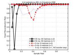
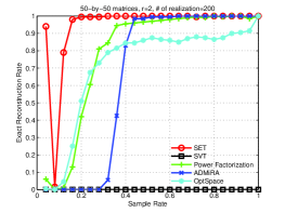
The performance of the SET algorithm is excellent. We tested different matrices with different ranks and different sampling rates, defined as $\left|\Omega\right|/\left(m\times n\right)$. The performance is shown in Fig. 2. The performance improvement due to the transfer step is significant. We also compare the SET algorithm to other matrix completion algorithms. As shown in Figure 3, the SET algorithm outperforms all other tested completion approaches. For most realizations, the SET algorithm needs less than 500 iterations to converge. However, there are examples for which the reconstruction error is still large after 2000 iterations. Studying such realizations indicates that the major reason for this phenomena is a slow convergence rate: after many iterations the barriers are still too far away from space $\bm{U}$ to be detectable. One future research direction is therefore to speed up the SET algorithm. As a final remark, we notice that there exist a critical range of sampling rates, in which the performance deteriorates. As can be observed from the figures, this range shifts to the right as the rank increases.

Figure 2: Performance of the SET algorithm.

Figure 3: Performance comparison.

References

- [1] J. Cai, E. J. Candes, and Z. Shen, “A singular value thresholding algorithm for matrix completion,” Oct. 2008.
- [2] K. Lee and Y. Bresler, “ADMiRA: atomic decomposition for minimum rank approximation,” Apr. 2009.
- [3] J. Haldar and D. Hernando, “Rank-constrained solutions to linear matrix equations using powerfactorization,” IEEE Signal Processing Letters, pp. 16:584–587, 2009.
- [4] R. H. Keshavan, A. Montanari, and S. Oh, “Matrix completion from a few entries,” 2009.
- [5] E. Candes and B. Recht, “Exact matrix completion via convex optimization,” Submitted for publication, 2008.
- [6] E. J. Candes and T. Tao, “The power of convex relaxation: Near-optimal matrix completion,” Mar. 2009.
- [7] W. Dai and O. Milenkovic, “Subspace pursuit for compressive sensing signal reconstruction,” IEEE Trans. Inform. Theory, vol. 55, pp. 2230 – 2249, May 2009.
- [8] D. Needell and J. A. Tropp, “CoSaMP: Iterative signal recovery from incomplete and inaccurate samples,” Applied and Computational Harmonic Analysis, vol. 26, pp. 301–321, May 2009.
- [9] A. Edelman, T. Arias, S. T. Smith, Steven, and T. Smith, “The geometry of algorithms with orthogonality constraints,” SIAM Journal on Matrix Analysis and Applications, vol. 20, pp. 303–353, April 1999.
- [10] P. E. Gill, W. Murray, and M. H. Wright, Practical Optimization. Academic Press, 1982.