Fractal Characterizations of MAX Statistical Distribution in Genetic Association Studies

ABSTRACT: Two non-integer parameters are defined for MAX statistics, which are maxima of $d$ simpler test statistics. The first parameter, $d_{MAX}$, is the fractional number of tests, representing the equivalent numbers of independent tests in MAX. If the $d$ tests are dependent, $d_{MAX}<d$. The second parameter is the fractional degrees of freedom $k$ of the chi-square distribution $\chi^{2}_{k}$ that fits the MAX null distribution. These two parameters, $d_{MAX}$ and $k$, can be independently defined, and $k$ can be non-integer even if $d_{MAX}$ is an integer. We illustrate these two parameters using the example of MAX2 and MAX3 statistics in genetic case-control studies. We speculate that $k$ is related to the amount of ambiguity of the model inferred by the test. In the case-control genetic association, tests with low $k$ (e.g. $k=1$) are able to provide definitive information about the disease model, as versus tests with high $k$ (e.g. $k=2$) that are completely uncertain about the disease model. Similar to Heisenberg’s uncertain principle, the ability to infer disease model and the ability to detect significant association may not be simultaneously optimized, and $k$ seems to measure the level of their balance.

1 Introduction

Geometric objects with non-integer dimensions such as coastal lines, random walk trajectories, Koch snowflakes have been well known [1]. Besides the feature of self-similarity, an important property of most fractals is their non-integer dimensionality. It is perhaps less known that non-integer or fractional parameter values is also a valid concept in statistical distributions. The best example is the fractional degrees of freedom ($df$). The $\chi^{2}$ (chi-square) distribution concerns the sum of squares of standard normal (Gaussian) variables. If $X_{1}$ and $X_{2}$ are two normally distributed variables with zero mean and unit variance, $Y=X_{1}^{2}+X_{2}^{2}$ is then distributed as the $\chi^{2}$ with two ($k=2$) degrees of freedom, denoted by $\chi^{2}_{k=2}$. The analytic expression of the probability density distribution of $\chi^{2}_{k}$ is known: $0.5^{k/2}/\Gamma(k/2)\cdot x^{k/2-1}exp{(-x/2)}$, where $\Gamma$ is the Gamma function [2]. In this expression, there is no conceptual difficulty to extend an integer value of $k$ to non-integers. However, since there is a specific meaning of $k$ in the original definition of chi-square distribution, i.e., the number of standard normal variables to be summed, one may wonder whether non-integer degrees of freedom, though allowed, have any applications.

The chi-square distribution plays an essential role in genetic association analysis, whose goal is to determine whether a genetic marker on a particular chromosome location is associated (correlated) with a human disease or presence/absence of a phenotype of interest [3, 4, 5]. The simplest genetic marker has two possible “values” (alleles), written as $a$ and $A$. Because half of the genetic material of a person is from the father (F), and another half from the mother (M), a marker configuration can be written as F$|$M. The two-allele marker has four possible configurations: $a|a,a|A,A|a$, and $A|A$. If we cannot distinguish the parental origin of an allele easily, as in the case with most technologies current in use, $A|a$ and $a|A$ are grouped into one configuration, and the resulting three configurations (after dropping the vertical bar), $aa,aA,AA$, are called genotypes.

The most popular design for genetic association study right now is the case-control design [6, 7, 8, 9, 10]. In this design, a group of patients (cases) and a group of disease-free normal persons (controls) are recruited, whose DNA molecules extracted, and their genotype throughout the genome (e.g. 10${}^{5}-10^{6}$ markers on 23 chromosomes) are determined (“genotyped”). For a particular marker, the number of case (and control) samples with the $aa,aA,AA$ genotypes are counted. These six genotype counts are stored in a 2-by-3 contingency table, rows for two disease status and columns for three genotypes. Many null hypothesis can be tested, and a significant violation of the null is used as evidence for genetic association between the marker and the disease. Exploration of the protein-coding genes near the marker could provide further insight into the mechanism for the disease.

Establishing the null hypothesis is not as easy as first thought. One obvious choice is to assume the three genotype frequencies to be unchanged in the two (case and control) groups. If we use the Peason’s chi-square test (goodness-of-fit test), the null distribution of the test statistic is $\chi^{2}_{k=2}$. The relation between the degree of freedom $k$ and the size of the contingency table is straightforward: $k$ is equal to the number of rows minus 1 multiplied by the number of columns minus 1 [11]. On the other hand, if the allele $A$ “dominates” allele $a$, there is no difference between the $aa$ and $aA$ genotypes; and after combining the $aa$ and $aA$ columns, the original 2-by-3 table becomes a 2-by-2 table, and the test statistic follows the $\chi^{2}_{k=1}$ null distribution. The similar collapses from 2-by-3 to 2-by-2 table could be carried out in several other ways, corresponding to “recessive”, “multiplicative”, “over-dominant”, etc. disease models, each has a $\chi^{2}_{k=1}$ null distribution for the corresponding test statistic.

If the disease model is known, i.e., if we know the disease risk given a genotype, one can easily choose the null hypothesis and a test so that deviation from the null could be detected. Unfortunately, for many complex human diseases, due to the multiple genes nature and gene-environment interaction, the disease model for a specific risk gene is largely unknown. To increase the chance to detect the association signal under the situation of model uncertainty, several tests, each testing a different null hypothesis, could be applied, and the best result among them is used. We call this procedure the “MAX test”. The MAX test that maximizes the test statistics from two or three disease models is a compromise between using one simple disease model and using no models. As a result, the null distribution of MAX test statistics is neither $\chi^{2}_{k=1}$ nor $\chi^{2}_{k=2}$, but something in between. We will show that this indeed leads to a fractional degrees of freedom $k$ for $\chi^{2}_{k}$, and $2-k$ measures our knowledge about the disease model. The determination of $k$ is complicated by another issue that sometimes the two or three test statistics being maximized are not independent. That leads to another fractional parameter: the number of independent tests $d_{MAX}$.

Although these two fractional parameters are not the same as the fractal dimension for fractals, a common theme is the non-integer value. We will explore the properties of these two parameters in details in this paper, organized as follows: Section 2 introduces statistical tests and MAX statistical test; Section 3 discusses the fractional number of tests for MAX test, from the perspective of family-wide $p$-values; Section 4 discusses the fractional degrees of freedom of chi-square distribution, from the perspective of fitting null distribution of MAX test statistics. In the discussion section, we address the issue on whether the fractional degrees of freedom is connected to fractal dimension in the parameter space.

2 MAX statistical test

When two different statistical tests are carried out on the same dataset [12], the more significant result of the two (i.e., the more extreme test statistic value) can be reported as the overall test result. This is a MAX statistical test. Clearly, MAX test statistic will always be larger than (or at least equal to) individual tests being maximized. Although the null distribution of a MAX test statistic may not be expressible by a simple analytic formula, we do expect the “center of gravity” of the distribution to be shifted to the right to have a larger mean and a thicker tail area (“inflated type I error”), as compared to that of a individual test, for the obvious reason that the maximization procedure increases the mean value.

Here we would like to define a MAX statistic for the case-control genetic association study. A dataset of such study consists of six numbers: number of case samples with $aa,aA,AA$ genotypes ($N_{10},N_{11},N_{12}$), and the number of control samples with these three genotypes ($N_{00},N_{01},N_{02}$) (see Appendix). The row $i$ in $N_{ij}$ indicates the case (1) or control(0) status, and column $j$ indicates the genotype with $j$ copies of $A$ allele.

We consider three different tests which are part of a test family called Cochran-Armitage trend ($CAT$) test [13, 14]. This family of tests is parameterized by a $x$ value, and the null hypothesis is the equality of weighted genotype frequency $xP_{aA}+P_{AA}$ in case and control group. When $x=0$, we are testing $P_{AA,case}=P_{AA,control}$, which corresponds to the genetic recessive model on the risk allele $A$. When $x=1$, we are testing the equality of $P_{aA}+P_{AA}$ in case and control group, which corresponds to genetic dominant model (whenever the risk allele $A$ is present in a genotype, the disease risk is the same regardless of the second allele). When $x=0.5$, we are testing the equality of the allele frequency, $P_{aA}/2+P_{AA}=P_{A}$, in the two groups.

The expression of $CAT$ test statistic is given in Appendix. There are other reformulation of the above formula, such as using the estimated allele frequency difference and Hardy-Weinberg disequilibrium coefficient difference [16], but the simplest calculation of $CAT(x=0)$ or $CAT(x=1)$ is to merge the $aA$ counts ($j=1$) with the $aa$ counts ($j=0$) or $AA$ counts ($j=2$), then calculate the Pearson’s chi-square test statistic (see Appendix).

If the underlying disease model is dominant, multiplicative, or recessive, the $CAT(x=1)$, $CAT(x=0.5)$, or $CAT(x=0)$, respectively, tends to be the largest. Fig.1 shows an example using a dominant model. The histogram determined by 100,000 replicates for $CAT(x=1)$ is peaked at the higher value than the other two $CAT$’s, $CAT(x=0.5)$ is distributed slightly lower than $CAT(x=1)$, whereas the distribution of $CAT(x=0)$ is far towards the smaller values.

If the disease model is unknown, it is when a MAX statistic is useful. One may consider these MAX statistics for case-control genetic data:

$$MAX2 \equiv max(CAT(x=0),CAT(x=1))$$ (1)

$$MAX3 \equiv max(CAT(x=0),CAT(x=0.5),CAT(x=1))$$

MAX2 was discussed in [15, 16], and MAX3 was discussed in [17, 18, 19]. Both MAX2 and MAX3 are “smart” samplings of the disease model space without an exhaustive search.

3 The fractional number of tests in calculating test-family wide $p$-values in MAX statistics

When several tests are applied to the same dataset and these tests are independent, there is a simple formula for calculating the test-family-wide $p$-value, which is also the $p$-value for the MAX test. We can derive the tail probabilities under the null distribution (i.e., $p$-value), $p_{MAX2}$ and $p_{MAX3}$, with the tail starting from the observed test statistic value $M$ by the following procedure ($p_{\chi^{2}}$ is the tail area probability under $\chi^{2}_{k=1}$ distribution):

$$p_{MAX2} \equiv P(MAX2>M|null)$$

$$= 1-P(MAX2<M|null)$$

$$= 1-P(CAT(x=0)<M~{}~{}and~{}~{}CAT(x=1)<M|null)$$

$$\approx 1-P(CAT(x=0)<M|null)\times P(CAT(x=1)<M|null)$$

$$= 1-(1-P(CAT(x=0)>M|null))\times(1-P(CAT(x=1)>M|null))$$

$$= 1-(1-p_{\chi^{2}})^{2}$$

$$p_{MAX3} \equiv P(MAX3>M|null)$$ (2)

$$= 1-P(MAX3<M|null)\approx\dots=1-(1-p_{\chi^{2}})^{3}.$$

The approximation can be replaced by the equal sign for MAX2 only if $CAT(x=0)$ and $CAT(x=1)$ are independent, and for MAX3 only if $CAT(x=0)$, $CAT(x=1)$ and $CAT(x=0.5)$ are independent. The independence assumption is untrue for MAX3 [17], but close to be true for MAX2 [16]. The two approximate formula in Eq.(3), also known as Dunn-S̆idák formula [20, 21], can be written as $1-(1-p_{\chi^{2}})^{d}$ for $d$ tests being maximized in MAX.

If we force the approximation sign in Eq.(3) to be equality, $d$ can be derived from $p_{MAX}$. This value of $d$ (called $d_{MAX}$ here) represents the effective number of independent tests:

$$d_{MAX}=\frac{\log(1-p_{MAX})}{\log(1-p_{\chi^{2}})}.$$ (3)

Note that the tail area probabilities for both MAX and chi-square, $p_{MAX}$ and $p_{\chi^{2}}$, are determined by the same $M$, the starting position of the tail area.

Besides multiple testing correction in test-family-wide $p$-value on the same dataset, the Dunn-S̆idak formula can also be used with the same test on multiple datasets. In particular, in whole genome association or linkage studies, selecting the SNP with the best association or linkage signal among $\sim 10^{5}$ SNPs belong to this application [22, 23], and the genome-wide $p$-value is calculated in the same way. The severe correction on $p$-value in this application is in a sharp contrast to the correction in Eq.(3), of a factor of only 2 or 3.

In order to estimate the effective number of tests for MAX2 and MAX3, we carried out the following simulation. We generated $N_{r}=$100,000 replicates, each replicate is a 2-by-3 genotype counts for 1000 cases and 1000 controls. The allele frequency is randomly chosen but the same allele frequency is used to simulate both case and control genotypes. The genotype frequency is derived from the allele frequency by the Hardy-Weinberg equilibrium. The empirical distribution of MAX2, MAX3, $CAT(x=0)$, $CAT(x=1)$, $CAT(x=0.5)$ can all be determined with 100,000 realizations of test statistic values (and the minimum $p$-value can’t be smaller than 1/100,000$=10^{-5}$). Using several threshold $M$ value (controlling type I error), $d_{MAX2}$ and $d_{MAX3}$ can be calculated by Eq.(3). Two more runs were also carried out with 3000 cases/3000 controls, and 5000 cases/5000 controls.

Fig.2 shows the empirical $d_{MAX2}$ and $d_{MAX3}$ as a function of $p_{\chi^{2}}$, the tail probability for the $\chi^{2}_{1}$ distribution. It can be seen that although there is only a slight reduction of $d_{MAX2}$ from the expected value of 2, $d_{MAX3}$ is much smaller than the expected value of 3. At $p_{\chi^{2}}=0.05$, the value of $d_{MAX3}$ is around 2.1, consistent with a similar result of $d_{MAX3}=2.2$ in [24].

The empirical $d$ values calculated from Eq.(3) for $CAT(x=1)$ and $CAT(x=0)$ are also shown in Fig.2 as a check of accuracy of the simulation. Indeed, the $d$ values do not deviate from the expected value of 1 with the exception at smaller $p_{\chi^{2}}$ values. For low $p_{\chi^{2}}$ values, a smaller number of replicates are used in the determination of the empirical $p$-values, thus variance is large – Fig.2 does show that the estimated $d_{MAX2}$ and $d_{MAX3}$’s are not consistent among the three runs at (e.g.) $p_{\chi^{2}}<0.01$, an indication of large run-to-run variation.

Another source of potential bias is that we keep the allele frequency a minimum distance away from the 0 value in order to avoid the situation of zero genotype count. The range of allele for these 3 runs are (0.1, 0.9), (0.05, 0.95), and (0.02, 0.98) respectively. Only when both the sample size and number of replicates go to infinity, and with unconstrained allele frequency, can one expect the simulation-based estimation of $d_{MAX}$ values to be exact.

4 Chi-square distributions with fractional degrees of freedom that fit the null distribution of Max test statistics

The second fractional parameter value related to the MAX concerns the fitting of MAX null distribution by a non-integer-$k$ $\chi_{k}^{2}$ distribution. As mentioned in Section 1, non-integer-$k$ chi-square distribution $\chi^{2}_{k}$ can be determined easily and is indeed implemented in statistical packages, such as $R$ (http://www.r-project.org/). Here we would like to check which $k$ value in $\chi_{k}^{2}$ leads to a better fit to the MAX null distribution.

In order to avoid confusion between $k$ and $d_{MAX}$, we made component tests to be independent so that $d_{MAX}$ remains an integer. Instead of generating case and control samples with specific genotype then calculate the MAX2, MAX3, $CAT(x=1)$ and $CAT(x=0)$, we randomly sample two, or three independent chi-square values from the $\chi^{2}_{k=1}$ distribution, then the maximization procedure is carried out. Due to the independence between chi-square values, $d_{MAX2}$ and $d_{MAX3}$ should be exactly equal to 2 or 3. Here we use a different notation, Max2 and Max3, to represent this correlation-free simulation (to be compared with Eq.(1):

$$Max2 \equiv max(\chi^{2}_{1},\chi^{2}_{1})$$

$$Max3 \equiv max(\chi^{2}_{1},\chi^{2}_{1},\chi^{2}_{1})$$ (4)

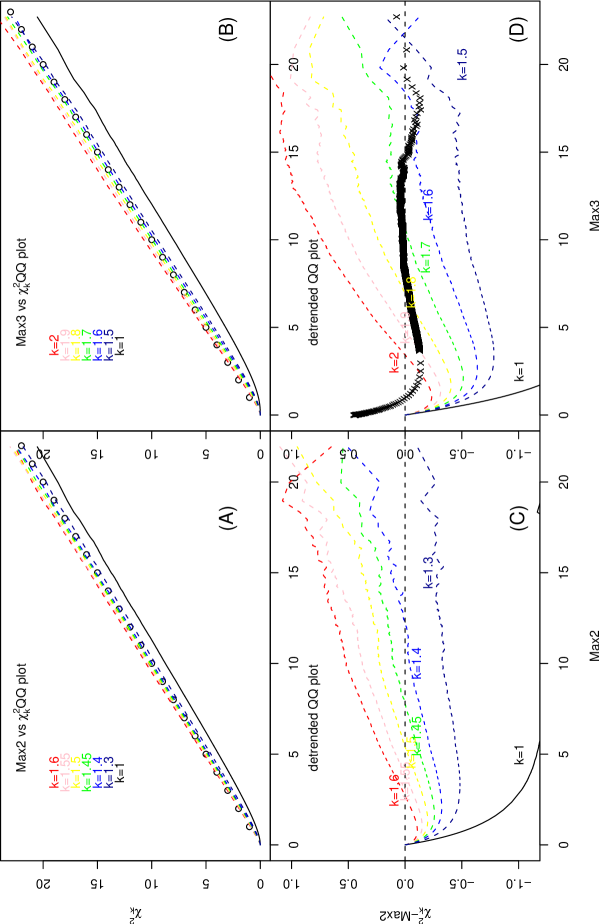
Figure 3: Quantile-quantile (QQ) plot of Max2/Max3 against values sampled from $\chi^{2}_{k}$ with fractional degrees of freedom $k$. (A) QQ plot of Max2 against values sampled from $\chi^{2}_{k}$’s with $k=1,1.3,1.4,1.45,1.5,1.55,1.6$. The circles indicate the QQ-plot between two identical distributions. (B) QQ plot of Max3 against values sampled from $\chi^{2}_{k}$’s with $k=1,1.3,1.5,1.6,1.7,1.8,1.9,2$. (C) Detrended QQ plot of Max2 against values sampled from $\chi^{2}_{k}$’s. (D) Detrended QQ plot of Max3 against values sampled from $\chi^{2}_{k}$’s. The crosses represent the detrended QQ-plot for $0.45+0.96\chi^{2}_{k=1.7}$ against Max3.

Fig.3 shows the result of fittings the empirical Max2 and Max3 by chi-square distribution with non-integer degree of freedoms. Fig.3(A,B) are the quantile-quantile (QQ) plot, where the $x$-axis is the ranked Max2 or Max3 value and $y$-axis is the ranked chi-square values with a fractional degrees of freedom ($k$=1.3, 1.4, 1.45, 1.5, 1.55, 1.6 for Max2, and $k$=1.5, 1.6, 1.7, 1.8, 1.9, 2 for Max3). To reduce variation, the average of 100 runs is used in Fig.3. When two distributions are identical, their QQ-plot should trace the diagonal line with slope=1 (marked by circles). In Fig.3(A,B) chi-square distribution with a range of fractional degrees of freedom seem to fit the Max2 and Max3 distribution well.

To examine more carefully how good fractional $k$ chi-square distributions fit the Max2/Max3 distribution, we draw the detrended QQ-plots in Fig.3(C,D), i.e., $y$-axis is the difference between the sorted chi-square values with fractional $k$ and the sorted Max2 or Max3 values. Fig.3(C,D) show systematic deviations between the two distributions. In other words, no chi-square distribution with one single fractional $k$ value may fit Max2 and Max3 for the entire range of values. For example, at Max2 $\approx 5$, $\chi^{2}_{1.5}-$ Max2$\approx 0$ (good fit), whereas when Max2 $>>5$, $\chi^{2}_{1.5}-$ Max2$>$0 (bad fit).

It is straightforward to determine which $\chi^{2}_{k}$ crosses the zero horizontal line at what position in Fig.3(C,D). First, from Eq.(3), we see a simple relationship between the “head area” of $\chi^{2}_{1}$ and that of Max2/Max3:

$$\sqrt{1-p_{Max2}} = 1-p_{\chi^{2}}$$

$$(1-p_{Max3})^{1/3} = 1-p_{\chi^{2}}.$$ (5)

The approximation in Eq.(3) becomes equality because MAX2/MAX3 is replaced by Max2/Max3. Here is an example in determining the zero crossing point in Fig.3(C): if the tail area $p_{Max2}$ for Max2 is 0.05, the “head area” is 0.95, and the corresponding head area for $\chi^{2}_{1}$ is $\sqrt{0.95}=0.9746794$. That head/tail area for $\chi^{2}_{1}$ can be used to determine the threshold value $M=5.001825$, as marked in Fig.4.

Then, we choose a $\chi^{2}_{k}$ with fractional $k$ so that its tail area determined by $M=5.001825$ is also 0.05. As shown in Fig.4, the threshold value for 0.05 area for $\chi^{2}_{1}$ is 3.841459 and that for $\chi^{2}_{2}$ is 5.991465. A fractional-$k$ $\chi^{2}_{k}$ ($1<k<2$) should have the threshold value for 0.05 tail area at $M=5.001825$. The exact $k$ can be iteratively determined by a bisection method, resulting in $k=1.51$. In other words, at $p_{Max2}=0.05$, $\chi^{2}_{k=1.51}$ is equivalent to the null distribution of Max2.

Fig.5(A) shows the above-mentioned fractional $k$ value vs. the tail area probability $p_{Max2}$ or $p_{Max3}$. We are mostly interested in small tail area values, e.g. $p_{Max2},p_{Max3}<0.05$, in a test. In this range, the equivalent fractional $k$ is constrained from above, e.g. smaller than 1.5 (1.85) for Max2 (Max3). We also attempt to convert the curve in Fig.5(A) to a straight line by variable transformation. This can be accomplished by taking the cubic root of $p_{Max2}$ or $p_{Max3}$: in Fig.5(B), the fractional $k$ vs. $p_{Max2}^{1/3}$ or $p_{Max3}^{1/3}$ exhibit a reasonably good linear trend.

Besides fitting the tail area of Max2/Max3 by a fractional-$k$ $\chi^{2}_{k}$, one may also use a $\chi^{2}_{k}$ that has the same average/mean as Max2 or Max3. We know that the average/mean of $\chi^{2}_{k}$ distribution is simply $k$, so this fractional dimension is very easy to determine. For example, in our simulation the means of Max2 and Max3 are 1.64 and 2.10 respectively. The corresponding fractional-$k$ $\chi^{2}_{k}$’s that have the same mean would be $\chi^{2}_{1.64}$ and $\chi^{2}_{2.10}$. Note that this fitting of Max2/Max3 by $\chi^{2}_{k}$ is to fit the mean which receives contribution from head as well as tail areas. It is not surprising that the resulting $k$’s are different from those that are based on tail areas only. Since the tail area is of major concern in most statistical inferences, we regard the definition of fractional $df$ from the tail area as more useful.

Figs.3-5 all illustrate that a single fractional-$k$ $\chi^{2}_{k}$ cannot fit the Max2/Max3 distribution perfectly. In particular, Fig.3(C,D) shows that the deviation between the two is directional: the matching $\chi^{2}_{k}$ has a fatter tail than Max2/Max3 beyond the crossing point. One method to remove the systematic deviation in Fig.3(C,D) is to use a linear function. For example, Fig.3(D) show the result when the $-0.45+0.04\chi^{2}_{k=1.7}$ linear trend is removed from the detrended QQ-plot of $\chi^{2}_{k=1.7}$ against Max3. It is equivalent to an approximation of sorted Max3 by $0.45+0.96sort(\chi^{2}_{k=1.7})$. Although it is not a perfect approximation, nor a unique one, the trend removal does reduce the systematic deviation.

5 Case-control genetic data

The result from the last section cannot be applied to the case-control data directly because the individual test statistics in Eq.1 are not independent, in particular for MAX3. There have been attempts to derive the null distribution of MAX3 by considering the joint distribution of $CAT(x=0)$, $CAT(x=0.5)$, and $CAT(x=1)$ [24, 25]. From Fig.3(B,D) and Fig.5(B), it is seen that we should not expect a single $\chi^{2}_{k}$ with a fractional $k$ to fit the MAX3 distribution perfectly.

The questions we asked for a real case-control data are: (1) what are the approximate values of $k$ if a $\chi^{2}_{k}$ is forced to fit the tail area probability of MAX3? (2) how good is our approximate distribution of Max3, 0.45+0.96 $\chi^{2}_{k=1.7}$, in fitting MAX3? For answering these questions, we use the case-control data for type 2 diabetes provided in [26].

The tail-area probability of MAX3 can be empirically obtained by permutation: the affection status label of samples are randomly shuffled, then the genotype counts are reconstructed. From such a genotype count table, the MAX3 value can be determined. Repeated calculation of MAX3 in label-shuffled dataset provides a null distribution, and from which one can derive the tail-area probability. The $p_{MAX3}$ thus determined for the top SNPs in [26] is reproduced in Table 1. From the permutation-derived $p_{MAX3}$, we find the best-fit $\chi^{2}_{k}$ that leads to the same $p_{MAX3}$ value, and that fractional degrees of freedom $k$ is listed in Table 1. A range of values of $k$ between 1.2 and 1.7, very similar to the range used in Fig.3(D).

Next, we estimate the tail area probability of MAX3 by an approximate formula discussed in the last section (and Fig.3(D)) for Max3. Due to the difference of Max3 and MAX3, and the approximation nature of the formula, we do not expect the derived tail area probabilities to be exact. Surprisingly, from the result in Table 1, this approximation actually leads to $p_{MAX3}$ that are similar to those obtained from permutation in [26].

Permutation only provides a sampling of the null distribution, and the finite number of replicates could be a source of error. Mimicking Fisher’s exact test, which determines the tail area probability by counting the number of states in the tail area by combinatorics, we can also determine the exact value of $p_{MAX3}$ (J. Tian, C. Xu, H. Zhang, Y. Yang, paper in preperation). This exact tail area probability is listed in the last column of Table 1. Again, we see that the approximation of $p_{MAX3}$ based on fractional-$k$ chi-square distribution isn’t far off from the exact values.

gene/SNP	MAX3	$p_{MAX3}$ (permutation)(1)	$k^{(2)}$	$p_{MAX3}$ (by $k=1.7$ formula)(3)	$p_{MAX}$ (exact)(4)
TCF7L2/rs7900150	34.18437	2.1 $\times 10^{-8}$	1.676	1.36 $\times 10^{-8}$	1.29 $\times 10^{-8}$
CAMTA1/rs1193179	25.71149	6.3 $\times 10^{-7}$	1.213	1.17 $\times 10^{-6}$	1.00 $\times 10^{-6}$
CXCR4/rs932206	23.28708	2.8 $\times 10^{-6}$	1.336	4.19 $\times 10^{-6}$	3.67 $\times 10^{-6}$
ZNF615/rs1978717	23.11983	4.9 $\times 10^{-6}$	1.595	4.57 $\times 10^{-6}$	4.01 $\times 10^{-6}$
HHEX/rs1111875	22.01918	8.6 $\times 10^{-6}$	1.597	8.17 $\times 10^{-6}$	7.82 $\times 10^{-6}$
LOC644419/rs282705	21.93485	9.0 $\times 10^{-6}$	1.598	8.54 $\times 10^{-6}$	6.27 $\times 10^{-6}$

Table 1: SNPs taken from the Table S4 of supplementary material of [26] with tail area probability (obtained from permutation) smaller than $10^{-5}$, and if more than SNPs in a gene are significant at this level, only one SNP is chosen here. The first two columns list the gene/SNP name and the MAX3 value (based on the genotype counts given in the supplementary material of [26]). (1) values of tail area probability provided by [26]; (2) the best fit of $k$ when the values in column “(1)” is used to fit a $\chi^{2}_{k}$ distribution; (3) estimation of the tail area probability of MAX3 by the distribution (for Max3) of 0.45+ 0.96$\chi^{2}_{k=1.7}$; (4) tail area probability of MAX3 by the exact enumeration of all possible combinations.

6 Discussion

In this paper, we introduce two fractional parameter values for MAX test statistics: (1) the fractional number of tests $d_{MAX}$ and (2) the fractional degree of freedom $k$ for the chi-square distribution that fits the Max null distribution. The parameter $d_{MAX}$ has its counterparts in other fields, such as the effective number of parameters for model selection [27, 28, 29, 30], effective number of genetic markers that are in linkage equilibrium [31, 32], effective number of grid points required to represent a climate field [33], effective sample size in genetic study for relatives [34], etc. It was stated in [35] that between the two extreme situations of two tests being independent and being identical, “an intermediate answer is to be anticipated”. In one particular situation, they actually have an example of 1.5 effective number of tests (page 340 of [35]).

There are two universal themes in these diverse studies: (1) Positive correlation causes the effective number to be smaller than the apparent number. This has several consequences, such as dimension reduction as a technique to simplify the dataset, correct ways for comparing statistical models by using the effective number of parameters to measure model complexity, etc. (2) As the effective number is determined from the real data, its value is most likely to be non-integer. Fractionality is the rule, not an exception.

The Bonferroni correlation of $p$-value for multiple testing is known to be conservative. The very reason that it is conservative is because tests can be positively correlated, which is also the cause for reduced values of effective number of tests. Various attempts were made to take into account of correlation among tests making a correction less conservative [36, 37, 38]. Our simulation results show that the reduction of effective number of tests for MAX2 is very small, indicating that $CAT(x=0)$ and $CAT(x=1)$ are not strongly correlated. However, there is a large reduction in the effective number of tests for MAX3, and the multiple factor of 3 is not appropriate in Bonferroni correction for MAX3.

Non-integer degrees of freedom $k$ for $\chi^{2}_{k}$ is our second fractional parameter, which had been encountered occasionally in statistical literature (e.g., [39]). The fact that $df$ can be non-integer is not surprising by itself, but it is more interesting to ask the question on whether it has any geometric interpretation. Our case-control association analyses example may provide a hint, as there is a tangible link between the $k$ value and the size of area in the disease model space.

A disease model can be specified by 4 parameters (see Appendix), but a projection from the 4-dimensional space to 2-dimensional one is possible. Using a 2-by-3 genotype count table as a realization of a disease model, Fig.6 shows two different ways to map a 2-by-3 genotype count table onto a two-dimensional plane. The first, as shown in Fig.6(A), uses the case-control difference of Hardy-Weinberg disequilibrium coefficients ($\delta_{\epsilon}$) and case-control difference of allele frequency ($\delta_{p}$) (see Appendix) [15, 16]. The second, as shown in Fig.6(B), uses the odd ratio of the baseline and heterozygote genotype ($OR_{1}$) and the odd ratio of the baseline and risk homozygote genotype ($OR_{2}$) (see Appendix) [40].

In the absence of constraints, randomly sampled disease model could scatter within a bounded plane in Fig.6 (an outer bound for Fig.6(A) could be: $-1\leq\delta_{p}\leq 1$, $-1/2\leq\delta_{\epsilon}\leq 1/2$), whereas disease models in a given class are located in a more restricted subspace, such as a line segment. We randomly sample dominant, recessive, multiplicative models and use them to generate dataset with 1000 case and 1000 control samples, these generated genotype count tables are mapping to 2-dimensional space in Fig.6. In Fig.6(A), multiplicative models are located along the $y$-axis as this model does not lead to Hardy-Weinberg disequilibrium; and recessive (dominant) models are located in regions with positive (negative) $\delta_{\epsilon}$ values [41, 15, 16]. Similarly, in Fig.6(B), dominant models are located along the line with slope 1 ($OR_{2}=OR_{1}$), multiplicative models are located in the line with slope 2 ($\log(OR_{2})/\log(OR_{1})=2$), and recessive models are on the vertical line ($OR_{1}=1$ and arbitrary $OR_{2}$).

If we sort different test statistics according to their corresponding degrees of freedom $k$ in $\chi^{2}_{k}$ for the null distribution, the following order appears: test on 2-by-3 genotype count table ($k=2$), MAX3 ($d\approx 1.57$), MAX2 ($d\approx 1.5$), $CAT(x=0.5)$ or $CAT(x=0)$ or $CAT(x=1)$ ($k=1$). On the projected disease model space in Fig.6, there is also a gradual narrowing of models for which these tests are designed to detect: genotype count test targets any models in the 2-dimensional space, MAX3 targets three types of models represented by 3 line segments, MAX2 targets two types of models represented by 2 line segments, and $CAT(x)$ targets only one line segments.

In Fig.6, the line segments for the three types of disease models are somewhat blurred into wider areas, but it is caused by random realization of datasets, rather than a manifestation of a fractal geometry. However, the fractional $df=k$ moves up from the integer value 1 to 1.5 and 1.57 when the number of line segments is increased. From this observation, we do not believe fractional $k$ is related to a fractional dimension of the underlying disease model subspace.

Even without a geometric interpretation, we may propose another meaning for $k$: $k-1$ can be used to measure the level of uncertainty in inferred disease model (mode of inheritance). For $CAT(x)$, $k-1=0$, and a significant test result also provides certain information concerning disease model. For genotype test, $k-1=1$ and a significant test does not tell us anything about the disease model. A significant MAX2 test result provides some information on disease model (for example, that the true model is unlikely to be multiplicative), whereas MAX3 offers even less information. If we consider the detection of association signal and inference of disease model as two independent tasks of a genetic association study, then these two components are reminiscent of those studied in the uncertainty principle in quantum physics [42], such as measuring the position and velocity of a particle at the same time.

In conclusion, MAX test provides an interesting example where two non-integer quantities can be defined and measured. The effective number of tests to be maximized is more straightforward and has appeared in other applications as well. The fractional-$k$ $\chi^{2}$ distribution for a test statistic is more intriguing, and seems to have a profound meaning concerning the test’s ability to infer specific information. We have shown that a linear function of fractional-$k$ $\chi^{2}$ distribution approximates the true distribution of MAX quite well. A hallmark of complex systems is its intermediate state between two extremes (order and disorder): a similarly intermediate state can also be described for fractional degrees of freedom in the MAX test which, in the genetic analysis context, sit between testing genetic association under completely specified and completely unknown disease models.

Appendix: Basic notations and results for case-control genetic tests

A case-control dataset consists of $N_{1}$ case samples and $N_{0}$ control samples whose genotype ($aa$ is the baseline homozygote, $aA$ is the heterozygote, $AA$ is the risk homozygote) is known. The dataset can be represented by a 2-by-3 genotype count table:

	aa	aA	AA	sample size
case(1)	$N_{10}$	$N_{11}$	$N_{12}$	$N_{1}=N_{1*}$
control(0)	$N_{00}$	$N_{01}$	$N_{02}$	$N_{0}=N_{0*}$
combined	$N_{*0}$	$N_{*1}$	$N_{*2}$	$N=N_{1}+N_{0}$

The above 2-by-3 genotype count table can be collapsed to several 2-by-2 tables. The following collapsing corresponds to a dominant model (the risk allele $A$ “dominates” allele “a”):

	aa	aA+AA
case(1)	$N_{10}$	$N_{11}$ + $N_{12}$
control(0)	$N_{00}$	$N_{01}$ + $N_{02}$

and the following collapsing corresponds to a recessive model (only two copies of the risk allele $A$ present a disease risk):

	aa+aA	AA
case(1)	$N_{10}$ + $N_{11}$	$N_{12}$
control(0)	$N_{00}$ + $N_{01}$	$N_{02}$

From a 2-by-2 table, Pearson’s chi-square test statistic $X^{2}$ is of the form of $\sum_{row,col}(O_{row,col}-E_{row,col})^{2}/E_{row,col}$ where $O_{row,col}$ is the observed (genotype) count is a table cell indexed by “row” and ”column”, and $E_{row,col}$ is the expected count. The expected count is equal to the product of the row margin $O_{row,*}=\sum_{col}O_{row,col}$ and the column margin $O_{*,col}=\sum_{row}O_{row,col}$. It can be shown that $X^{2}$ is the product of squared matrix determinant and total sample size divided by the product of 4 row and column margins (e.g., [15]). For example, for the recessive model, $X^{2}$ is:

$$D = (N_{10}+N_{11})N_{02}-(N_{00}+N_{01})N_{12}$$

$$X^{2}_{REC} = \frac{D^{2}N}{(N_{*0}+N_{*1})N_{*2}N_{1}N_{0}}$$ (6)

Under the null hypothesis (by chance alone), $X^{2}$ follows the $\chi^{2}_{k=1}$ distribution (chi-square distribution with one degree of freedom). $X^{2}_{DOM}$ can be calculated similarly.

The Cochran-Armitage trend ($CAT$) test is defined after each genotype is assigned a score. Most assignment of the genotype score could be equivalent to a score of $\{x_{i}\}\equiv(0,x,1)$, i.e., the score for the baseline homozygote is fixed at 0, that for the risk homozygote is fixed at 1, and that for the heterozygote is a parameter $x$. The $CAT$ test statistic at $x$ is defined as ([43, 44, 19]:

$$CAT(x)=\frac{N_{1*}N_{0*}}{N}\frac{\left(\sum_{j=0}^{2}x_{j}(N_{1j}/N_{1*}-N_{0j}/N_{0*})\right)^{2}}{\left(\sum_{j=0}^{2}x_{j}^{2}N_{*j}/N-(\sum_{j=0}^{2}x_{j}N_{*j}/N)^{2}\right)}$$

It can be shown that $CAT(x=0)$ is equal to $X^{2}_{REC}$ and $CAT(x=1)$ is equal to $X^{2}_{DOM}$. Under the null hypothesis, $CAT(x)$ at each fixed $x$ value follows the $\chi^{2}_{k=1}$ distribution.

A disease model of a bi-allelic disease locus can be specified by 4 parameters. One is the allele frequency ($p\equiv p_{A}$) and the other three characterize the susceptibility of the disease under each genotype: $(f_{0},f_{1},f_{2})\equiv(P(disease|aa),P(disease|Aa),P(disease|AA))$. The latter three parameters can be replaced by the following three parameters: relative genotype risk for heterozygote: $\lambda_{1}\equiv f_{1}/f_{0}$, that for the risk homozygote, $\lambda_{2}\equiv f_{2}/f_{0}$, and disease prevalence $K=f_{0}[(1-p)^{2}+\lambda_{1}2p(1-p)+\lambda_{2}p^{2}]$. Either a ($p_{A},f_{0},f_{1},f_{2}$) value or a ($p_{A},\lambda_{1},\lambda_{2},K$) value uniquely determines a disease model.

There are several ideas in reducing the number of parameters of a disease model from 4 to 2 “major” parameters. One suggestion [15] is to use the allele frequency difference in case and in control group $\delta_{p}\equiv p_{A}(case)-p_{A}(control)=p_{1}-p_{0}$, and Hardy-Weinberg disequilibrium coefficient difference in the two groups $\delta_{\epsilon}\equiv\epsilon(case)-\epsilon(control)=\epsilon_{1}-\epsilon_{0}$. The Hardy-Weinberg disequilibrium coefficient $\epsilon$ measures the deviation from Hardy-Weinberg equilibrium [3], such that the three genotype frequencies can be written as ($(1-p)^{2}+\epsilon$, $2p(1-p)-2\epsilon$, $p^{2}+\epsilon$). The motivation for this parameterization is that $\delta_{p}$ is directly related to the case-control association signal, and $\delta_{\epsilon}$ is strongly correlated with the disease model.

The group-specific allele frequency and Hardy-Weinberg disequilibrium coefficient can be determined from the 4 parameters $p,\lambda_{1},\lambda_{2},K$ [41], and their differences can be determined as well [16]:

$$\delta_{p}\equiv p_{1}-p_{0} = \frac{f_{0}(p^{2}\lambda_{2}+p(1-p)\lambda_{1})}{K}-\frac{p^{2}(1-f_{0}\lambda_{2})+p(1-p)(1-f_{0}\lambda_{1})}{1-K}$$

$$\delta_{\epsilon}\equiv\epsilon_{1}-\epsilon_{0} = \frac{f_{0}^{2}p^{2}(1-p)^{2}(\lambda_{2}-\lambda_{1}^{2})}{K^{2}}-\frac{f_{0}p^{2}(1-p)^{2}(2\lambda_{1}-1-\lambda_{2}-f_{0}\lambda_{1}^{2}+f_{0}\lambda_{2})}{(1-K)^{2}}.$$

Given a 2-by-3 genotype table, these two parameters can be estimated by:

$$\hat{\delta}_{p} = \hat{p}_{1}-\hat{p}_{0}=\frac{N_{12}+N_{11}/2}{N_{1}}-\frac{N_{02}+N_{01}/2}{N_{0}}$$

$$\hat{\delta}_{\epsilon} = \hat{\epsilon}_{1}-\hat{\epsilon}_{0}=\frac{N_{12}}{N_{1}}-\left(\frac{N_{12}+N_{11}/2}{N_{1}}\right)^{2}-\frac{N_{02}}{N_{0}}+\left(\frac{N_{02}+N_{01}/2}{N_{0}}\right)^{2}.$$

Another idea in selecting two major parameters in the disease model is to ignore $p$ and $K$, and focus only on $\lambda_{1}$ and $\lambda_{2}$. These two parameters can be estimated by the two odd-ratios from subtables consisting of one baseline column and another risk column:

$$\hat{\lambda_{1}}=OR_{1} = \frac{N_{11}N_{00}}{N_{10}N_{01}}$$

$$\hat{\lambda_{2}}=OR_{2} = \frac{N_{12}N_{00}}{N_{10}N_{02}}.$$

Fig.6(A) and (B) illustrate these two ideas of a two-dimensional disease model space.

Figure 1: The distribution of $CAT(x=1)$, $CAT(x=0.5)$ and $CAT(x=1)$ from the 100,000 replicates generated by a dominant model: population risk allele frequency $p=0.1$, penetrance for baseline homozygote is 0.005, and genotype relative risk for both heterozygote and the risk homozygote is $\lambda_{1}=\lambda_{2}=2$. The genotype frequency for the case and the control group is calculated by the formula given in [41].

Figure 2: Fractional number of tests for MAX2 and MAX3 ($d_{MAX2},d_{MAX3}$) determined by Eq.(3) with three simulation runs, as a function of tail area probability under $\chi^{2}_{1}$ ($p_{\chi^{2}_{1}}$). Each run contains 100,000 replicates of genotype count tables for 1000 cases and 1000 controls (3000 cases/3000 controls, 5000 cases/5000 controls for the second and the third run). As a comparison, the effective number of tests for $CAT(x=0)$ and for $CAT(x=1)$ as determined by simulation is also included. As expected, these effective number of tests is essentially equal to 1.

Figure 4: Probability density distribution of $\chi^{2}_{1}$ (labeled by 1), $\chi^{2}_{2}$ (labeled by 2), $\chi^{2}_{k=1.51}$ (dashed line), and simulated Max2 (solid line). The threshold value $M$’s that correspond to tail area of 0.05 for these distributions are also marked. The $\chi^{2}_{k=1.51}$ distribution has the same $M$ as the Max2 distribution, so the two are equivalent at the tail area of 0.05.

Figure 5: (A) The fractional degrees of freedom $k$ of $\chi^{2}_{k}$ that is equivalent to Max2 and Max3 at tail area $\alpha$ as a function of $\alpha$. (B) $k$ is plotted versus $\alpha^{1/3}$.

Figure 6: Simulation of 100 case-control datasets each for three classes of models (dominant, multiplicative, recessive). Each point represents a genotype count table for 1000 cases and 1000 controls. The allele frequency is randomly chosen from (0.1-0.9); disease prevalence is sampled from the normal distribution with a random mean, and standard deviation of 1/10 of the mean; the $\lambda_{2}$ genotype relative risk is randomly chosen between (1.1-10); $\lambda_{1}$ is equal to $\lambda_{2}$, $\sqrt{\lambda_{2}}$, and 1 for dominant, multiplicative, and recessive models. (A) The location of simulated datasets in the $\delta_{\epsilon}$-$\delta_{p}$ parameter space, where $\delta_{\epsilon}$ is the case-control difference of Hardy-Weinberg disequilibrium coefficients and $\delta_{p}$ is the case-control difference of allele frequencies. The symbols “d”, “m”, “r” represent dominant, multiplicative, and recessive models, respectively. (B) The location of the same simulated case-control datasets in the $OR_{1}$-$OR_{2}$ space (both $x$ and $y$-axis are in log scale), where $OR_{1}$ is the odd-ratio of heterozygote genotype vs. baseline homozygote genotype, and $OR_{2}$ is the odd-ratio of risk homozygote genotype vs. baseline homozygote genotype.

References

- [1] B.B. Mandelbrot (1983), The Fractal Geometry of Nature (W.H. Freeman).
- [2] W.H. Press, B.P. Flannery, S.A. Teukolsky, W.T. Vetterling (1988), Numerical Recipes in C (Cambridge University Press).
- [3] B.S. Weir (1996), Genetic Data Analysis II (Sinauer Associates).
- [4] P. Sham (1997), Statistics in Human Genetics (Hodder Arnold Publication).
- [5] D.C. Thomas (2004), Statistical Methods in Genetic Epidemiology (Oxford University Press).
- [6] N. Risch, K. Merikangas (1996), “The future of genetic studies of complex human diseases”, Science, 273:1516-1517.
- [7] H.J. Cordell, D.G. Clayton (2005), “Genetic Epidemiology 3: Genetic association studies”, Lancet, 366:1121-1131.
- [8] J.N. Hirschhorn, M.J. Daly (2005), “Genome-wide association studies for common diseases and complex traits”, Nature Rev. Genet., 6:95-108.
- [9] D.J. Balding (2006), “A tutorial on statistical methods for population association studies”, Nature Rev. Genet., 7:781-791.
- [10] W. Li (2008), “Three lectures on case-control genetic association analysis”, Brief. in Bioinf., 9:1-13.
- [11] A. Agresti (2002) Categorical Data Analysis, 2nd edition (Wiley).
- [12] R.G. Miller (1981), Simultaneous Statistical Inference, 2nd edition (Springer-verlag, NY).
- [13] W.G. Cochran (1954), “Some methods of strengthening the common tests”, Biometrics, 10:417-451.
- [14] P. Armitage (1955), “Tests for linear trends in proportions and frequencies”, Biometrics, 11:375-386.
- [15] Y.J. Suh, W. Li (2007), “Genotype-based case-control analysis, violation of Hardy-Weinberg equilibrium, and phase diagram”, in Proceedings of the 5th Asia-Pacific Bioinformatics Conference, eds. D Sankoff, L Wang, F Chin, pp.185-194 (Imperial College Press).
- [16] W. Li, Y.J. Suh, Y. Yang (2008), “Exploring case-control genetic association tests using phase diagram”, Comp. Biol. Chem, 32:391-399.
- [17] B. Freidlin, G. Zheng, Z. Li, J.L. Gastwirth (2002), “Trend tests for case-control studies of genetic markers: power, sample size and robustness”, Hum. Hered., 53(3):146-152.
- [18] G. Zheng (2003), “Use of max and min scores for trend tests for association when the genetic model is unknown”, Stat. in Med., 22:2657-2666.
- [19] G. Zheng, B. Freidlin, J.L. Gastwirth (2006), “Comparison of robust tests for genetic association using case-control studies”, in ed. J Rojo Optimality: The Second Erich L. Lehmann Symposium, pp. 253-265 (IMS).
- [20] H.K. Ury (1976), “A comparison of four procedures for multiple comparisons among means (pairwise contrasts) for arbitrary sample sizes”, Technometrics, 18:89-97.
- [21] R.K. Sokal, F.J. Rohlf (1995), Biometry, 3rd edition (W.H. Freeman and Company, New York).
- [22] E.S. Lander, L. Kruglyak (1995), “Genetic dissection of complex traits: guidelines for interpreting and reporting linkage results” Nature Genet., 11:241-247.
- [23] B Efron (2004), “Large-scale simultaneous hypothesis testing: the choice of a null hypothesis”, J. Am. Stat. Asso., 99:96-104.
- [24] J.R. González, J.L. Carrasco, F. Dudbridge, L. Armengol, X. Estivill, V. Moreno (2008), “Maximizing association statistics over genetic models”, Genet. Epid., 32:246-254.
- [25] Q. Li, G. Zheng, Z. Li, K. Yu (2008), “Efficient approximation of p-value of the maximum of correlated tests, with applications to genome-wide association studies”, Ann. Hum. Genet., 72:397-406.
- [26] R. Sladek, G. Rocheleau, J. Rung, C. Dina, L. Shen, D. Serre, P. Boutin, D. Vincent, A. Belisle, S. Hadjadj, B. Balkau, B. Heude, G. Charpentier, T.J. Hudson, A. Montpetit, A.V. Pshezhetsky, M. Prentki, B.I. Posner, D.J. Balding, D. Meyre, C. Polychronakos, P. Froguel (2007), “A genome-wide association study identifies novel risk loci for type 2 diabetes”, Nature, 445:881-885.
- [27] J. Moody (1992), “The effective number of parameters: an analysis of generalization and regularization in nonlinear learning systems”, in eds. Moody, Hanson, Lippmann Advances in Neural Information Processing Systems 4, pp. 847-854 (Morgan Kaufmann, Palo Alto, CA).
- [28] J. Mao, A.K. Jain (1997), “A note on the effective number of parameters in nonlinear learning systems”, Neural Networks, 2:1045-1050.
- [29] J. Ye (1998), “On measuring and correcting the effects of data mining and model selection”, J. Am. Stat. Asso., 93:120-131.
- [30] D.J. Spiegelhalter, N.G. Best, B.P. Carlin, A. Van der Linde (2002), “Bayesian measures of model complexity and fit”, J. Roy. Stat. Soc. B, 64(4):583-616.
- [31] J.M. Cheverud (2001), “A simple correction for multiple comparisons in interval mapping genome scans”, Heredity, 87:52-58.
- [32] D.R. Nyholt (2004), “A simple correction for multiple testing for single-nucleotide polymorphisms in linkage disequilibrium with each other”, Am. J. Hum. Genet., 74:765-769.
- [33] C.S. Bretherton, M. Widmann, V.P. Dymnikov, J.M. Wallace, I. Bladé (1999), “The effective number of spatial degrees of freedom of a time-varying field”, J. Climate, 12(7):1990-2009.
- [34] Y. Yang, E.L. Remmers, C. Ogunwole, D. Kastner, P.K. Gregersen, W. Li (2007), “Effective sample size: quick estimation of the effect of related samples in genetic case-control association analyses”, Nature Precedings preprint, hdl:10101/npre.2007.400.1.
- [35] A. Azzalini, D.R. Cox (1984), “Two new test associated with analysis of variance”, J. Roy. Stat. Soc. B, 46:335-343.
- [36] R.J. Simes (1986), “An improved Bonferroni procedure for multiple tests of significance”, Biometrika, 73:751-754.
- [37] B. Efron (1997), “The length heuristic for simultaneous hypothesis tests”, Biometrika, 84:143-157.
- [38] Y. Ninomiya, H. Fujisawa (2007), “A conservative test for multiple comparison based on highly correlated test statistics”, Biometrics, 63:1135-1142.
- [39] J.A. Doornik, H. Hansen (2008), “An omnibus test for univariate and multivariate normality”, Oxford Bull. Econ. Stat., 70:927-939.
- [40] G. Zheng, H.K.T. Ng (2008), “Genetic model selection in two-phase analysis for case-control association studies”, Biostatistics, 9:391-399.
- [41] J.K. Wittke-Thompson, A. Pluzhnikov, N.J. Cox (2005), “Rational inferences about departures from Hardy-Weinberg equilibrium”, Am. J. Hum. Genet., 76:967-986.
- [42] W. Heisenberg (1930), The Physical Principles of Quantum Theory (University of Chicago Press).
- [43] P.D. Sasieni (1997), “From genotypes to genes: doubling the sample size”, Biometrics, 53(4):1253-1261.
- [44] S.L. Slager, D.J. Schaid (2001), “Case-control studies of genetic markers: power and sample size approximations for Armitage’s test for trend”, Hum. Hered., 52:149-153.