Stochastic Langevin equations: Markovian and non-Markovian dynamics

Abstract

Non-Markovian stochastic Langevin-like equations of motion are compared to their corresponding Markovian (local) approximations. The validity of the local approximation for these equations, when contrasted with the fully nonlocal ones, is analyzed in details. The conditions for when the equation in a local form can be considered a good approximation are then explicitly specified. We study both the cases of additive and multiplicative noises, including system dependent dissipation terms, according to the Fluctuation-Dissipation theorem.

Published: Physical Review E80, 031143 (2009)

I Introduction

Most systems in nature cannot be regarded as purely closed systems but open ones, interacting with an environment (e.g. a thermal bath). The evolution of these systems must then be non unitary, i.e., interactions with the environment must lead to dissipation as well stochastic effects, which is the way the environment backreacts on the system. One common way for describing this non unitary evolution is by means of stochastic Langevin-like equations of motion. These non-deterministic equations of motion are used in many systems of interest, such as simulating Brownian motion in (classical and quantum) statistical mechanics and in other areas of physical interest reviews .

A classical example of a system whose dynamics is modeled by a Langevin equation of motion is the one that describes the Brownian motion of a classical particle of coordinate $q$, unitary mass and subjected to a potential $V(q)$ (as usual dots mean derivative with respect to time and $V^{\prime}[q(t)]\equiv dV/dq$),

$$\ddot{q}(t)+\eta\dot{q}(t)+V^{\prime}[q(t)]=\xi(t)\;,$$ (1)

where $\eta$ is a Markovian (local) dissipation term and $\xi(t)$ is a stochastic term with white noise and Gaussian properties, satisfying (throughout this work we consider the Boltzmann constant $k_{B}=1$)

$$\langle\xi(t)\rangle=0\;,\;\;\;\langle\xi(t)\xi(t^{\prime})\rangle=2T\eta\delta(t-t^{\prime})\;.$$ (2)

Approaches with Langevin equations such as Eq. (1) and its generalizations, are used in different contexts, e.g. in classical statistical mechanics to study problems with dissipation and noise, to determine how order parameters equilibrate and in the studies such as dynamic scaling and dynamic critical phenomena critical ; critical2 .

Though extensively used, equations of the form of Eq. (1), with noise properties as given by Eq. (2), can only be considered phenomenologically. This is because it implicitly assumes that the environment interacts instantaneously with the system. This is a physically unacceptable situation that violates causality, since the environment bath has no memory time. Its is worth mentioning that a similar situation happens with the description of the dynamics of a conserved order parameter by a Cahn-Hilliard equation CH , which lacks causality Jou1 . In the case of the Cahn-Hilliard equation this happens because, since it is a diffusion-reaction type of equation, it should be characterized by microscopic scattering events. In real systems scattering events proceed through finite time intervals, which, consequently, must lead to finite memory effects. In order to fix this bad behavior of the Cahn-Hilliard equation, memory effects must be taken into account, as explicitly shown recently in Ref. KKR . In a microscopic description of the effects of the environment degrees of freedom on some select variables taken as the system, the same is expected to happen. Dissipation and stochastic (noise) terms are expected to originate from scattering events, thus giving origin to finite interaction times, that reflect in the system’s equation of motion as nonlocal (i.e. non-Markovian) terms with memory effects. The simplest archetype of this is the description of the system-environment as being modeled by linearly coupled harmonic oscillators oscillators (for a general review, see e.g. Ref. weiss ), which also become to be known as Caldeira-Leggett type of models caldeira . The derived equation of motion for the system variable, when the bath degrees of freedom are integrated out, leads to a generalized Langevin equation (GLE) of the form

$$\ddot{q}(t)+\int_{t_{0}}^{t}dt^{\prime}D(t-t^{\prime})\,\dot{q}(t^{\prime})+V^{{}^{\prime}}[q(t)]=\xi(t)\;,$$ (3)

where $t_{0}$ is some initial time, $D(t-t^{\prime})$ is a dissipation kernel and the noise term $\xi(t)$ is still Gaussian with zero mean but colored, i.e., with two-point correlation, according to the Fluctuation-Dissipation theorem for classical systems, and, thus $\xi(t)$ satisfies

$$\langle\xi(t)\rangle=0\;,\;\;\;\left\langle\xi(t)\xi(t^{\prime})\right\rangle=TD(t-t^{\prime})\;,$$ (4)

where averages are assumed to be taken with respect to a bath of free oscillators with equilibrium distribution $\rho_{B}^{(0)}$ at some temperature $T$. Similar derivations in the context of field theory models (see, for instance Refs. GR ; BMR ) also show the emergence of generalized equations of motion of the form of Eq. (3), with a more complicated structure depending on the form of the coupling of the system (e.g. some field we are interested in the dynamics) with the environment (or bath fields, made of the remaining fields other than the one representing the system field).

Despite the fundamental differences between Eqs. (1) and (3), we expect that when the time scale of the memory kernel $D(t-t^{\prime})$ is much smaller than any other time scales of the system, the local approximation (1), with dissipation coefficient defined by ingold ; hanggi

$$\eta=\int_{-\infty}^{t}dt^{\prime}D(t-t^{\prime})\;,$$ (5)

can still be a good approximation for the system’s dynamics and the effects of finite memory be negligible. There is also an immense saving of effort as well as much more transparent understanding of the physics from a local equation as opposed to a nonlocal one, since the former can generally be analyzed with much less numerical treatment than the latter, thus it is a very important question to know when, and how accurately, a generally nonlocal equation can be approximated by a local form. Likewise, when the memory constrains cannot be ignored, such as when the typical microscopic time scales are large in comparison to the other time scales characterizing the dynamics, we must then be able to have appropriate tools to tackle the non-Markovian equations of motion. This is possible with some restrict forms of kernels, as we are going to see below, which, nevertheless, can represent physically relevant systems of interest, thus, being well motivated.

In this work our objective is to gauge the applicability of an equation of motion of the form of Eq. (1) when compared to the non-Markovian form, when considering some of the most common forms for the dissipation kernel $D(t,t^{\prime})$. These forms for the dissipation kernel include for example the one that describes an Ornstein-Uhlenbeck (OU) process OUref and the exponential damped harmonic (EDH) kernel EDHref (see also Ref. Luczka for a recent review on the different colored noise terms used in the literature). We study both the cases of additive and multiplicative noises, including system dependent dissipation terms, according to the Fluctuation-Dissipation theorem. A detailed numerical analysis is made when the various parameters characterizing the thermal bath, e.g. the bath relaxation (or damping) parameter, frequency and temperature of the bath are varied.

The remaining of this work is organized as follows. In Sec. II we define the prescription to transform the non-Markovian equations in a system of Markovian time differential equations. We study specifically the OU and EDH kernels. In Sec. III we present the numerical results for the non-Markovian equations for different model parameters and compare the results to those coming from their Markovian approximations. The results are obtained for both the cases of additive and multiplicative noises. How the dynamics depends on the various parameters characterizing the thermal bath is studied in details. In Sec. IV we present our conclusions, discuss the various results we have obtained, and we give a possible relation and the relevance of our results for the study of nonequilibrium dynamics in field theory models.

II The non-Markovian Langevin-like Equation

Here we study a GLE describing the interaction of a system, denoted by a variable $\phi$ (which can be e.g. the coordinate of a particle) in interaction with a thermal bath, where the noise has the properties such as in Eq. (4). The GLE studied here is then of the generic form

$$\ddot{\phi}(t)+\phi^{n}(t)\int_{t_{0}}^{t}dt^{\prime}\phi^{n}(t^{\prime})D(t-t^{\prime})\,\dot{\phi}(t^{\prime})+V^{\prime}(\phi)=\phi^{n}(t)\,\xi(t)\;,$$ (6)

where $n=0,1$, with $n=0$ giving the standard GLE of additive form, such as Eq. (3), while for $n=1$ gives a multiplicative GLE. The multiplicative noise and system dependent dissipation form are motivated from field theory calculations GR ; BMR and this is why we have also included this special case here in view of future applications in that case. The potential in Eq. (6) is considered to be one with quadratic and quartic terms, given by

$$V(\phi)=\frac{m^{2}}{2}\phi^{2}+\frac{\lambda}{4!}\phi^{4}\;,$$ (7)

where $m^{2}$ and $\lambda$ are parameters depending on the details of the system under study. Here, we can associate $m$ with the system’s frequency and $\lambda$ with the degree of nonlinearity of the system’s potential (or in the context of field theories, with the strength of the system’s self-interactions).

Nonlinear GLEs of the form of Eq. (6) are notably difficult to solve. Analytical methods can only be used when the equation can be approximated or put in a linear form, such as in the additive noise case and when the quartic term in the system’s potential can be neglected. This is because, in the additive noise and variable independent dissipation case, such as in Eq. (3), the equation is in the form of a convolution, so can be solved through Laplace transform for instance CPC2008 . Otherwise, in the more general cases, we must resort to numerical methods. This is the approach we follow in this paper in order to analyze the dynamics obtained from Eq. (6). Though there are some specific numerical methods using e.g. Fourier transform that may apply for equations with non-Markovian kernels of generic form bao1 , we still would like to be able to solve equations such as Eq. (6) through standard methods, which are less numerically expensive than other alternatives. This is the case, for example, when using Runge-Kutta methods. Recently, the authors CPC2008 have demonstrated the reliability of using a fourth-order Runge-Kutta method when solving GLE of the OU and EDH forms. The way this can be done stems from the fact that non-Markovian equations with kernels of those forms can be replaced by a system of completely local first-order differential equations, which has been described in details in CPC2008 .

As already mentioned, in this work we concentrate our study in equations such as Eq. (6) with non-Markovian kernels of either the OU type OUref

$$D_{OU}(t-t^{\prime})=\eta\,\gamma e^{-\gamma(t-t^{\prime})}\;,$$ (8)

or with the EDH type EDHref

$$D_{H}(t-t^{\prime}) = \eta\,e^{-\gamma(t-t^{\prime})}\frac{\Omega_{0}^{2}}{2\gamma}\left\{\cos[\Omega_{1}(t-t^{\prime})]\right.$$ (9)

$$+ \left.\frac{\gamma}{\Omega_{1}}\sin[\Omega_{1}(t-t^{\prime})]\right\}\;,$$

where in the equations above, $\eta$ sets the magnitude of the dissipation, $\gamma$ sets the relaxation time for the bath kernels, $\tau=1/\gamma$, and $\Omega_{0}$ gives the oscillation time scale in the case of the EDH kernel. In Eq. (9), $\Omega_{1}^{2}=\Omega_{0}^{2}-\gamma^{2}$, and so, in the EDH case the values of $\gamma$ and $\Omega_{0}$ are restricted so to have $\Omega_{1}^{2}\geq 0$.

It can be easily shown that the OU and EDH noises can be generated by the stationary part of the solution of the following differential equations, respectively,

$$\dot{\xi}_{OU}(t)=-\gamma\left[\xi_{OU}(t)-\sqrt{2T\eta}\,\zeta(t)\right]\;,$$ (10)

$$\ddot{\xi}_{H}(t)+2\gamma\dot{\xi}_{H}(t)+\Omega_{0}^{2}\xi_{H}(t)=\Omega_{0}^{2}\sqrt{2T\eta}\,\zeta(t)\;,$$ (11)

where $\zeta$ in Eqs. (10) and (11) is a white Gaussian noise satisfying

$$\langle\zeta(t)\rangle = 0\;,$$

$$\langle\zeta(t)\zeta(t^{\prime})\rangle = \delta(t-t^{\prime})\;.$$ (12)

Taking $t_{0}=0$, we can define a new variable $w(t)$ by bao2 ; CPC2008

$$w(t)=-\int_{0}^{t}dt^{\prime}\phi^{n}(t^{\prime})D(t-t^{\prime})\dot{\phi}(t^{\prime})\;.$$ (13)

This, together with Eqs. (10) and (11), leads to the following system of local first-order differential equations representing the GLE Eq. (6): For the OU case,

$$\dot{\phi} = y\;,$$

$$\dot{y} = -V^{\prime}(\phi)+\phi^{n}w_{OU}+\phi^{n}\xi_{OU}\;,$$

$$\dot{w}_{OU} = -\gamma w_{OU}-D_{OU}(0)\phi^{n}y\;,$$

$$\dot{\xi}_{OU} = -\gamma\left[\xi_{OU}-\sqrt{2T\eta}\,\,\zeta\right]\;,$$ (14)

while for the EDH case we obtain

$$\dot{\phi} = y\;,$$

$$\dot{y} = -V^{\prime}(\phi)+\phi^{n}w_{H}+\phi^{n}\xi_{H}\;,$$

$$\dot{w}_{H} = u-2\gamma w_{H}-D_{H}(0)\,\phi^{n}y\;,$$

$$\dot{u} = -\Omega_{0}^{2}w_{H}+\dot{D}_{H}(0)\,\phi^{n}y-2\gamma D_{H}(0)\,\phi^{n}y\;,$$

$$\dot{\xi}_{H} = z\;,$$

$$\dot{z} = -2\gamma z-\Omega_{0}^{2}\xi_{H}+\Omega_{0}^{2}\sqrt{2T\eta}\,\zeta\;,$$ (15)

where the variable $u(t)$ in Eq. (15) is defined as

$$u(t)=\int_{0}^{t}dt^{\prime}\left[\frac{dD_{H}(t-t^{\prime})}{dt^{\prime}}-2\gamma D_{H}(t-t^{\prime})\right]\phi^{n}(t^{\prime})\frac{d\phi(t^{\prime})}{dt^{\prime}}\;,$$ (16)

and in Eqs. (14) and (15), we also have that $D_{OU}(0)=\eta\,\gamma$, $D_{H}(0)=\eta\,\Omega_{0}^{2}/(2\gamma)$ and $\dot{D}_{H}(0)=0$, which follow from Eqs. (8) and (9). The additive noise case is when $n=0$ is taken in Eqs. (14) and (15), while $n=1$ is for the multiplicative noise case. These two cases, for both types of kernels, are next numerically studied below.

III Contrasting the non-Markovian numerical results with the Markovian approximation ones

Let us now consider our numerical results for the Markovian and non-Markovian dynamics for the system. In the Markovian approximation all memory effects are neglected and the non-Markovian dissipation term in Eq. (6) is replaced by a local dissipation term with magnitude as given by Eq. (5), i.e., we write Eq. (6) in the form

$$\ddot{\phi}(t)+\eta\,\phi^{2n}(t)\,\dot{\phi}(t)+V^{\prime}(\phi)=\phi^{n}(t)\,\xi(t)\;.$$ (17)

As we have mentioned before, in general we expect the local form the GLE to be a valid approximation when the relaxation time scale for the thermal bath, $\tau=1/\gamma$, is much smaller than the characteristic time scale for the system, e.g., $\tau\ll\phi/\dot{\phi}$ (this is equivalent to the quasi-adiabatic condition set in Ref. GR in the field theory case for the validity of the local Markovian approximation). When this condition is met in a sufficiently large time interval $\Delta t=t-t_{0}$, thus $\Delta t/\tau\gg 1$ (which is equivalent as taking $t_{0}\to-\infty$) and the time nonlocal term in Eq. (6) can be written as

$$\phi^{n}(t)\int_{t_{0}}^{t}dt^{\prime}D(t-t^{\prime})\phi^{n}(t^{\prime})\,\dot{\phi}(t^{\prime})$$

$$\simeq\phi^{2n}(t)\,\dot{\phi}(t)\int_{t_{0}\to-\infty}^{t}dt^{\prime}D(t-t^{\prime})\to\eta\,\phi^{2n}(t)\,\dot{\phi}(t)\;,$$ (18)

where in the last step we have used the definition Eq. (5). The result (18) then leads to the local dissipation term in Eq. (17). Of course, under the conditions set above, at sufficiently short times we expect the memory effects to influence the dynamics in some significant way, but these memory effects should quickly become negligible at long times, $t\gg 1/\gamma$. In any event, we thus expect that after some long time period the memory effects can become sufficiently damped such that the Markovian approximation could represent well the overall dynamics of the system. After all, we expect that both dynamics, the non-Markovian and the Markovian ones to both have the same asymptotic state. But we still face with a natural and important question to answer: For a given set of model parameters representing the system and the thermal bath to which it is coupled to, for how long can we expect the memory effects due to the non-Markovian terms to be important and when can they be neglected and then the dynamics be well represented by the local Eq. (17) ? This is because, even though both dynamics are expected to approach each other asymptotically, the time this happens could be so long that the memory effects could lead to important physical effects and the local Markovian dynamics would just not be appropriate to be used. Since the representation of the dynamics in a local form as given by Eq. (17) represents a considerable simplification, for both a numerical point of view, or for analytical analysis (when it is possible), when compared, e.g., to the full nonlocal, integro-differential stochastic Eq. (6), this then becomes an important question to be accessed for most practical studies that make use of stochastic equations of motion. It is also important to investigate how the dynamics is affected by varying not only $\gamma$, but the other parameters characterizing the thermal bath, such as the temperature $T$ and frequency $\Omega_{0}$, whose effects on the dynamics may not so direct as the ones obtained by just varying $\gamma$. Below we try to answer all these questions, performing our study, numerically, in the context of the additive and multiplicative noise cases, with either the OU or EDH kernel terms, defined in the previous section.

Next we show the results of our systematic simulations of the system of differential first-order equations, Eqs. (14) and (15), for the non-Markovian GLE with OU and EDH kernels, respectively. The results are compared to those obtained through the local approximation given by Eq. (17). All our simulations were performed with $300\,000$ realizations over the noise and we have integrated all differential equations using a standard fourth-order Runge-Kutta method with a time stepsize varying between $\delta t=0.01$ and $\delta t=0.001$, which were found to be more than enough for both numerical stability and also for enough numerical precision (as determined in Ref. CPC2008 , these values already assure an overall numerical error of always smaller than about one percent, which suffices for our comparison purposes set here). In all our simulations we have also used the initial conditions $\phi(0)=1$ and $\dot{\phi}(0)=0$. The time in all our evolutions is in units of the (inverse of the) frequency for the system (which is equivalent to consider $m=1$ throughout). Comparisons between the Markovian and non-Markovian dynamics are made varying the relevant parameters of the bath for the two cases of kernels considered, while keeping the system parameters fixed.

III.1 The additive noise case

Figure 1: OU case with additive noise and its Markovian approximation: time evolution for $\varphi(t)$. (a) $\gamma=0.5$, (b) $\gamma=1.0$ and (c) $\gamma=5.0$. The other parameters are taken as $\Omega_{0}=1.0$, $\eta=1.0$, $T=1.0$, $m=1.0$ and $\lambda=1.0$.

Figure 2: EDH case with additive noise and the Markovian approximation: time evolution for $\varphi(t)$. (a) for $\gamma=0.1$, (b) for $\gamma=0.3$ and (c) for $\gamma=0.5$. The other parameters are the same as in Fig. 1.

Let us now turn to our numerical results. The relevant bath parameters are the dissipation magnitude $\eta$, the temperature $T$ (that are common to both Markovian and non-Markovian dynamics), the bath damping parameter $\gamma$, and the bath frequency $\Omega_{0}$ (in the EDH kernel case). Since the dissipation magnitude is common for both types of dynamics, in the following we keep $\eta$ fixed, at the value $\eta=1$ throughout (which can be checked to correspond to lead to an underdamped dynamics in the local equations of motion) and we vary the remaining bath parameters. This will allow us to better understand the importance of the memory effects alone for the dynamics. So, we consider the various dynamics as $\gamma$, $\Omega_{0}$ and $T$ are changed. We include the study of how the dynamics changes with the temperature because this is useful to determine how this internal property of the thermal bath influences the dynamics when comparing to both the Markovian and non-Markovian cases.

We start our analysis by first considering variations in the parameter $\gamma$. Representative values for $\gamma$ are then chosen and all the remaining parameters are initially kept fixed. Note that since $\gamma$ acts as damping the effects of the nonlocal kernels, the larger is $\gamma$ the better must be the local approximation for the full nonlocal dynamics. Then we keep $\gamma$ fixed at the largest value used in our analysis and then consider variations in the other parameters. This will allow us to determine the consequent importance of the remaining parameters and whether a change of those parameters can discriminate the types of dynamics studied, for example discriminate additive and multiplicative stochastic dynamics.

Let us first consider the GLE with additive noise and OU kernel. This is considered in Fig. 1, where we plot side by side our results for the dynamics of the ensemble averaged macroscopic system variable $\phi$, $\langle\phi\rangle=\varphi(t)$, where the average is over the noise realizations. This is obtained from the Markovian and non-Markovian equations, Eqs. (17) and (14), respectively, with $n=0$.

In Fig. 2 we plot side by side our results for $\varphi(t)$ for the Markovian and non-Markovian regimes for the EDH case, again by considering the additive noise ($n=0$).

The effect of changing $\gamma$ seen in both Figs. 1 and 2 is clear and well within the expected: The larger is the relaxation time ($1/\gamma$) for the nonlocal kernels, the larger are the memory effects, resulting in a strong difference with respect to the local approximation, seen most notably at short times. As also expected, at some sufficient long time, that we here see to depend on how large $\gamma$ is, the two dynamics, Markovian and non-Markovian approximate one of the other. This is also seen if we had plotted the correlation $\langle\phi^{2}(t)\rangle$ for both OU and EDH cases. The difference between the Markovian and non-Markovian dynamics can also be better estimated by defining the quantities,

$$\Delta\phi = \langle\phi\rangle_{\rm non-Markovian}-\langle\phi\rangle_{\rm Markovian}\;$$

$$\Delta\phi^{2} = \langle\phi^{2}\rangle_{\rm non-Markovian}-\langle\phi^{2}\rangle_{\rm Markovian}\;.$$ (19)

The results for the differences $\Delta\phi$ and $\Delta\phi^{2}$ are shown in Figs. 3 and 4, for the OU and EDH cases, respectively.

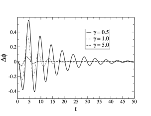
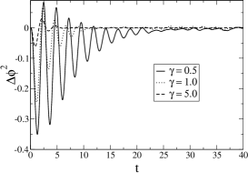
Figure 3: The differences $\Delta\phi$ and $\Delta\phi^{2}$ in the OU additive case. All other parameter kept fixed as before.

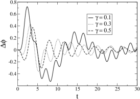
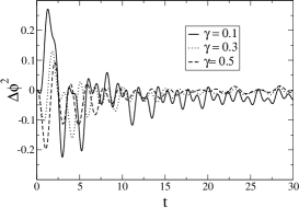
Figure 4: The differences $\Delta\phi$ and $\Delta\phi^{2}$ in the difference $\Delta\phi^{2}$ in the EDH additive case.

The results from the plots shown in Figs. 3 and 4 are useful to determine within which time scale the Markovian and non-Markovian dynamics become sufficiently close (within to some given precision). The results for these time scales for the different simulations we have performed for the Markovian dynamics and for the non-Markovian dynamics with the two types of memory kernels explored here will be given below in Table 1.

An immediate conclusion we can realize from an inspection of the results shown in Figs. 1 - 4 is that the time scale that it takes for the two dynamics to begin to be equivalent is much larger than the time scale for the kernel relaxation itself, $1/\gamma$, and also larger than the typical system’s time scale, which is typically given by the inverse of the system’s frequency ($1/m$). This will remain true for the multiplicative noise case with either the OU or the EDH memory kernels.

III.2 The multiplicative noise case

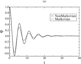
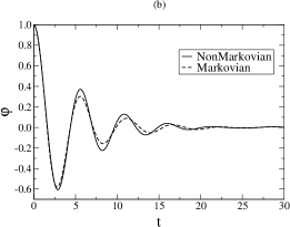
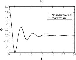
Figure 5: OU case with multiplicative noise and its Markovian approximation: time evolution for $\varphi(t)$. (a) for $\gamma=0.5$, (b) for $\gamma=1.0$ and (c) for $\gamma=5.0$. The other parameters are taken as $\Omega_{0}=1.0$, $\eta=1.0$, $T=1.0$ and $\lambda=1.0$.

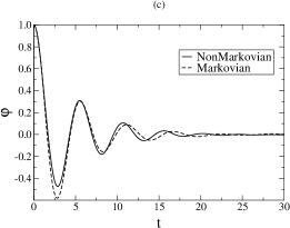
Figure 6: EDH case with multiplicative noise and the Markovian approximation: time evolution for $\varphi(t)$. (a) for $\gamma=0.1$, (b) for $\gamma=0.3$ and (c) for $\gamma=0.5$. All other parameters taken as in the previous figures.

Let us now verify the results concerning the Markovian and non-Markovian stochastic equations when multiplicative noise and system dependent dissipation are concerned. We then here explore the case $n=1$ in Eqs. (14) and (15), for the OU and EDH cases, respectively.

In Fig. 5 we plot side by side our results for $\langle\phi\rangle$ for the Markovian and non-Markovian regimes in the OU case with $n=1$, while in Fig. 6 are the results for the EDH case.

The results for the differences $\Delta\phi$ and $\Delta\phi^{2}$, for the $n=1$ multiplicative noise case, are shown in Figs. 7 and 8, for the OU and EDH cases, respectively.

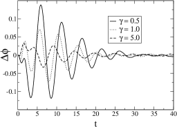
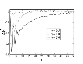
Figure 7: The differences $\Delta\phi$ and $\Delta\phi^{2}$ for the OU multiplicative case. All other parameter kept fixed as before.

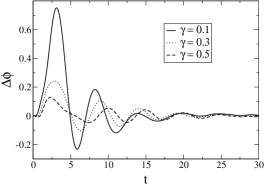
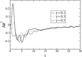
Figure 8: The differences $\Delta\phi$ and $\Delta\phi^{2}$ for the EDH multiplicative case.

The results shown in Figs. 5 - 8 again indicate that, as expected and similar to the additive noise $n=0$ case, that the two dynamics, local and nonlocal, become closer to each other the larger is the kernel damping parameter. They also seem to indicate that in the multiplicative noise case the two dynamics are closer to each other for the same parameters used in the additive noise case. This can be more quantitatively estimated through the differences (19). The results for the time scales when the two dynamics begin to be sufficiently close to each other are also presented in Table 1.

$\gamma$	$\Delta\phi_{\rm OU\;add}$	$\Delta\phi^{2}_{\rm OU\;add}$	$\Delta\phi_{\rm OU\;mult}$	$\Delta\phi^{2}_{\rm OU\;mult}$
0.5	73	28	35	70
1.0	32	25	30	24
5.0	14	7	27	12

$\gamma$	$\Delta\phi_{\rm EDH\;add}$	$\Delta\phi^{2}_{\rm EDH\;add}$	$\Delta\phi_{\rm EDH\;mult}$	$\Delta\phi^{2}_{\rm EDH\;mult}$
0.1	180	89	30	73
0.3	67	33	28	71
0.5	53	26	23	67

Table 1: The approximate time scale, in units of $1/m$, for the non-Markovian dynamics to approach the Markovian one, within a precision of $10^{-3}$ for the differences defined in (19).

We note from the results shown in Table 1 that the system variable $\phi$ in the case of the GLE with OU additive noise tends to approximate the corresponding Markovian dynamics faster than in the case of the multiplicative noise case. The opposite seems to happen to the equal time correlation function $\langle\phi^{2}\rangle$, where in the case of OU multiplicative noise it is faster than in the case of additive noise. The behavior of $\Delta\phi$ in the additive noise cases indicates that the averaged system variable $\langle\phi\rangle$ is approached faster to the Markovian dynamics than in the multiplicative noise cases. The behavior for the dynamics of $\langle\phi^{2}\rangle$, when looking at the behavior of $\Delta\phi^{2}$, is analogous, except in the EDH multiplicative noise case, where it is slower than in the additive noise case.

In addition to the above results obtained for the ensemble average system variable $\phi$, it is also useful to determine how the memory effects influence the thermalization time for the system when put in contact with the thermal bath at some temperature $T$. For this, let us define an effective time dependent temperature for the system according to the equipartition of kinetic energy,

$$T_{\rm eff}(t)=\langle\dot{\phi}^{2}(t)\rangle\;.$$ (20)

The results for $T_{\rm eff}$ for the OU and EDH cases for the additive and multiplicative noise situations are shown in Fig. 9, where it is also plotted the Markovian, local approximation case, for comparison.

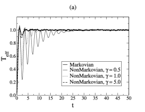
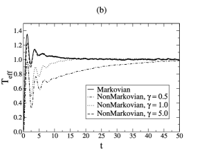
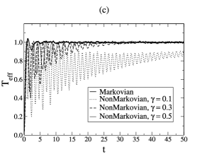
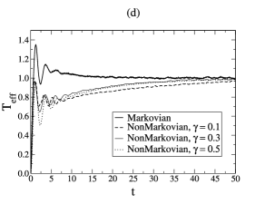
Figure 9: The effective temperature $T_{eff}$ for the (a) OU $n=0$ case, (b) OU $n=1$ case, (c) EDH $n=0$ case and (d) EDH $n=1$ case.

From the plots shown in Fig. 9 we again see the overall behavior seen in the previous plots. The larger is the relaxation time for the memory kernels (i.e., the smaller is the damping parameter $\gamma$ of the memory kernels), the larger the dynamics takes to approach the Markovian approximated one. We also see how memory effects reflects in the thermalization of the system. Larger bath relaxation times lead to a longer time for the system to thermalize. Typically, for comparable bath relaxation time scales, in the additive case the system tends to thermalize faster than in the multiplicative case. In Table 2 we give the approximate time (in units of $1/m$) for thermalization for all the cases studied above and where this behavior for the time for thermalization in each of the types of dynamics analyzed can be verified. Note that in all cases, with additive or multiplicative noise, the Markovian dynamics tend in general to underestimate the time scale for thermalization, when compared to the non-Markovian dynamics, except for large $\gamma$ in the OU additive noise case, where the thermalization in the non-Markovian dynamics tends to be better approximated by the Markovian one. As far the different dynamics are concerned, we observe from both the plots in Fig. 9 as from the results shown in Table 2 for the thermalization times, that the additive noise case always tend to have a smaller thermalization time than the multiplicative noise case. This is observed for both the Markovian and non-Markovian cases.

$\gamma$	$\tau_{\rm markov\;add}$	$\tau_{\rm OU\;add}$	$\tau_{\rm markov\;mult}$	$\tau_{\rm OU\;mult}$
0.5		37		72
1.0	4	18	27	68
5.0		4		38

$\gamma$	$\tau_{\rm markov\;add}$	$\tau_{\rm EDH\;add}$	$\tau_{\rm markov\;mult}$	$\tau_{\rm EDH\;mult}$
0.1		152		126
0.3	4	39	27	77
0.5		33		74

Table 2: The approximate time for thermalization, in units of $1/m$, for the Markovian and non-Markovian dynamics, determined when (20) approaches the temperature of the thermal bath.

III.3 Markovian and non-Markovian dynamics in terms of the temperature of the thermal bath

We now explore how the temperature of the thermal bath will influence the results shown in the previous section. We again concentrate on the differences between the Markovian and non-Markovian dynamics and the thermalization time. For this study we consider the cases with the highest values of $\gamma$ considered in the previous subsection, which gives the best comparison between the dynamics. Keeping the highest values of $\gamma$ allows us to determine whether the comparison between the two dynamics improves or worsens as the temperature is changed.

The results for the differences $\Delta\phi$ and $\Delta\phi^{2}$ for the GLE with OU kernel are shown in Fig. 10, while for the GLE with EDH kernel are shown in Fig. 11. The time scale for which the full non-Markovian dynamics approaches the respective Markovian dynamic approximation, in each of the cases studied here, are tabulated in Table 3.

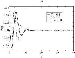
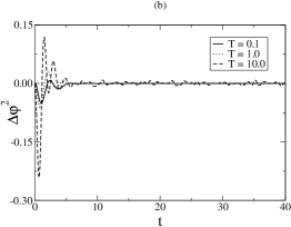
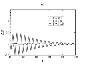
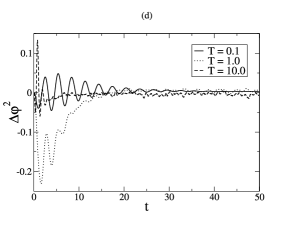
Figure 10: The results for $\Delta\phi$ and $\Delta\phi^{2}$ for the OU $n=0$ case, (a) and (b), respectively, and for the OU $n=1$ case, (c) and (d), respectively.

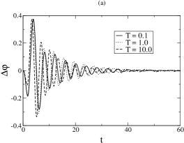
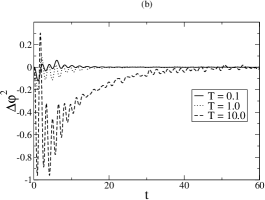
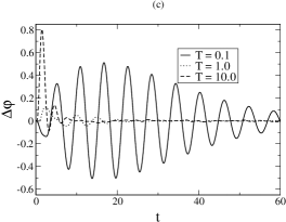
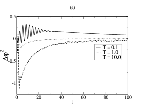
Figure 11: The results for $\Delta\phi$ and $\Delta\phi^{2}$ for the EDH $n=0$ case, (a) and (b), and for the EDH $n=1$ case, (c) and (d).

$T$	$\Delta\phi_{\rm OU\;add}$	$\Delta\phi^{2}_{\rm OU\;add}$	$\Delta\phi_{\rm OU\;mult}$	$\Delta\phi^{2}_{\rm OU\;mult}$	$\Delta\phi_{\rm EDH\;add}$	$\Delta\phi^{2}_{\rm EDH\;add}$	$\Delta\phi_{\rm EDH\;mult}$	$\Delta\phi^{2}_{\rm EDH\;mult}$
0.1	17	10	140	206	68	24	126	220
1.0	14	7	27	12	53	26	23	67
10.0	13	6	6	7	42	49	13	61

Table 3: The approximate time scale, in units of $1/m$, for the non-Markovian dynamics to approach the Markovian one, within a precision of $10^{-3}$ for the differences defined in (19) for different temperatures for the thermal bath. The parameter $\gamma$ considered is the largest one considered in Table 1 in the OU ($\gamma=5.0$) and EDH cases ($\gamma=0.5$).

From the results shown in Table 3 we can see that higher temperatures for the thermal bath give only minor improvements in the OU additive noise case as regarding the approach of the non-Markovian dynamics to the approximated Markovian one. But in the multiplicative (OU) case the changes are much stronger, with $\langle\phi\rangle$ and $\langle\phi^{2}\rangle$ approaching much faster to the Markovian dynamics the larger is the temperature. In the EDH case, for the additive noise, $\langle\phi\rangle$ tends to approach slower to the Markovian approximation and in the multiplicative noise case the approach is much faster, compared to the additive one. But the correlation $\langle\phi^{2}\rangle$ changes much differently. In the EDH additive noise case the Markovian approximation worsens as the temperature is increased, while in the multiplicative case the Markovian approximation improves, but only slightly for high temperatures. Similar behavior to this will also be seen below for the thermalization times for each of the dynamics. We can also observe from the results shown in the plots of Figs. 10 and 11 that for the multiplicative noise case, for both non-Markovian dynamics studied, the memory effects are much stronger at lower temperatures than at high temperatures and these effects last for a much longer time than in the additive noise cases.

We now study how the thermalization time for each of the dynamics studied here will change when the temperature is changed. In Fig. 12 we show the plots for the various cases of dynamics studied here. The thermalization times for each case are tabulated in Table 4.

 

 

 

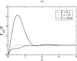
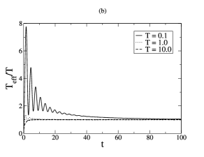
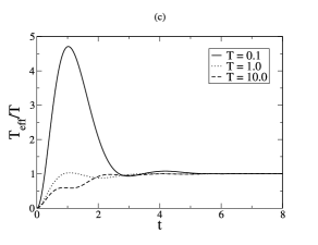
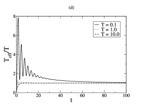
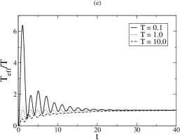
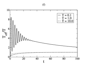
Figure 12: The results for the effective temperature as a function of time, when the temperature of the thermal bath is changed, for the cases of (a) Markovian additive noise, (b) Markovian multiplicative noise, (c) OU additive noise, (d) OU multiplicative noise, (e) EDH additive noise and (f) EDH multiplicative noise.

$T$	$\tau_{\rm markov\;add}$	$\tau_{\rm markov\;mult}$	$\tau_{\rm OU\;add}$	$\tau_{\rm OU\;mult}$	$\tau_{\rm EDH\;add}$	$\tau_{\rm EDH\;mult}$
0.1	7	123	6	135	30	570
1.0	4	27	4	38	33	74
10.0	6	9	7	15	48	65

Table 4: The approximate time for thermalization, in units of $1/m$, for the Markovian and non-Markovian dynamics, determined when (20) approaches the temperature of the thermal bath.

From the results shown in the plots of Fig. 12 and in Table 4, we can clearly see that while the cases with OU noise the thermalization times for the Markovian and non-Markovian dynamics are similar (using the largest values of $\gamma$ considered in Table 1), the non-Markovian dynamics with EDH noise, for both the additive and multiplicative cases, produces thermalization times considerably larger than those of the Markovian cases. As in the case of $\Delta\phi^{2}$ for the EDH additive noise case seen in Table 3, we again see here the anomalous behavior of the thermalization time increasing as the temperature is increased in the EDH additive noise case. This is opposite to the behavior seen in the OU and EDH noise cases with multiplicative noise. Note also that in the case closer to the Markovian dynamics, the OU additive noise case, there is almost no relevant difference in thermalization times as the temperature is varied up to 2 orders of magnitude. For other values of temperature of the thermal bath we tested, we found that these conclusions do not change.

III.4 The non-Markovian dynamics in terms of the frequency of the thermal bath

We now investigate how the frequency of the thermal bath affects the dynamics of the system. Note that in this case only the GLE with EDH kernel is affected (the Markovian and OU dynamics are independent of the frequency of the thermal bath). As before, we can better interpret the results by analyzing the differences (19) and the graph of the effective temperature. From them we obtain the time scale for the non-Markovian dynamics to approach the Markovian one and we can better estimate the differences in thermalization times (if any) in both cases. The results for this case, when the frequency of thermal bath is varied, are shown in Fig. 13 for the differences (19), while the behavior of the effective temperature, when the frequency of the bath is changed, is shown in Fig. 14. In all cases the frequency $\Omega_{0}$ is in units of the frequency of the system, $m$, and the time is in units of $1/m$. As in the previous analysis for the EDH case, we consider $\gamma=0.5$, and all other parameters kept fixed at the values as given before, except $\Omega_{0}$. The time scales for the non-Markovian and Markovian dynamics to approach to each other are given in Table 5, while the time for thermalization for each case is given in Table 6.

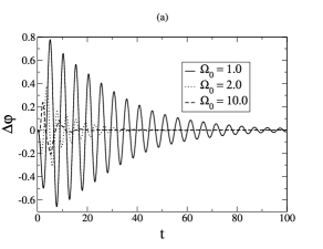
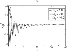
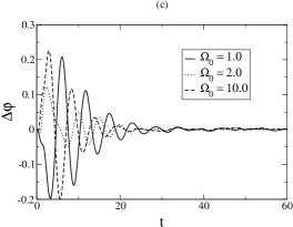
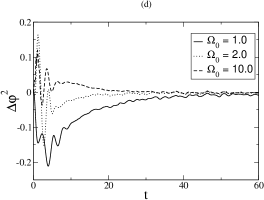
Figure 13: The results for $\Delta\phi$ and $\Delta\phi^{2}$, when the frequency of the thermal bath (in units of $m$) is changed, for the EDH $n=0$ case, plots (a) and (b), respectively, and for the EDH $n=1$ case, plots (c) and (d), respectively.

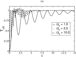
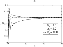
Figure 14: The results for the effective temperature as a function of time, when the frequency of the thermal bath (in units of $m$) is changed, for the cases of (a) EDH additive noise and (b) EDH multiplicative noise.

$\Omega_{0}/m$	$\Delta\phi_{\rm EDH\;add}$	$\Delta\phi^{2}_{\rm EDH\;add}$	$\Delta\phi_{\rm EDH\;mult}$	$\Delta\phi^{2}_{\rm EDH\;mult}$
1.0	53	26	23	67
2.0	24	8	25	38
10.0	22	8	25	33

Table 5: The approximate time scale, in units of $1/m$, for the non-Markovian dynamics to approach the Markovian one, within a precision of $10^{-3}$ for the differences defined in (19) for different frequencies of the thermal bath. The parameter $\gamma$ considered is the largest one considered in Table 1 in the EDH cases ($\gamma=0.5$).

$\Omega_{0}/m$	$\tau_{\rm markov\;add}$	$\tau_{\rm markov\;mult}$	$\tau_{\rm EDH\;add}$	$\tau_{\rm EDH\;mult}$
1.0			33	74
2.0	4	27	13	8
10.0			9	35

Table 6: The approximate time for thermalization, in units of $1/m$, for different frequencies of the thermal bath in the in the Markovian approximation and in the EDH additive and multiplicative noise cases.

From the results seen in Fig. 13 and Table 5 we can note that the smaller is the frequency of the thermal bath the larger it takes for both $\langle\phi\rangle$ and $\langle\phi^{2}\rangle$ in the non-Markovian case to approach the Markovian approximation. As the frequency of the bath is increased beyond the frequency of the system, the time scale for the non-Markovian dynamics to approach the Markovian one tends to decrease, but it also rapidly reaches a point where larger frequencies for the bath would not make the Markovian approximation to improve too much.

The results are seen to be much different again when the thermalization of the system is studied. From the thermalization plots seen in Fig. 14 and the thermalization times given in Table 6, we see that smaller frequencies for the bath, compared to the system’s frequency, lead to much higher thermalization times for the non-Markovian approximation compared to the Markovian one. The thermalization time for the non-Markovian dynamics is seen to decrease with an increase of $\Omega_{0}$, except the multiplicative noise case, where above a certain point $\Omega_{0}\gtrsim m$, the thermalization time starts to increase again. Though the importance of the memory kernel is expected to be less important the larger is $\Omega_{0}$, which makes it fast oscillate, the behavior in the multiplicative noise is probably far less simple, because the higher are the nonlinearities in that case, which are brought by the system dependent dissipation and noise.

IV Conclusions

In this work we have analyzed in details the differences between the dynamics of a system when treating it in terms of its full non-Markovian equation of motion and when expressing it in terms of its Markovian, or local approximated form. Having set the appropriate description for the non-Markovian equations, we have then studied the applicability of the local approximation for these equations. We here have concentrated in two forms for the non-Markovian memory kernel: The OU and EDH cases and we have analyzed the cases of additive and multiplicative noises in both cases. We have seen that in general, for most of the parameters in both cases, the local approximation is far from being to represent a good description of the dynamics. Obviously, since these are all dissipative systems, we expect the two dynamics, non-Markovian and Markovian, to tend to each other asymptotically. We have then analyzed how long it takes for each of the non-Markovian dynamics studied to tend to the Markovian ones. We have analyzed both the time for the system variable, $\langle\phi\rangle$, as well for the equal time correlation, $\langle\phi^{2}\rangle$. We have also analyzed the thermalization time for each of the dynamics by studying the behavior of the correlation function $\langle\dot{\phi}^{2}\rangle$, which, according to the equipartition theorem, can be associated to the temperature of equilibration of the system.

Each of the dynamics were investigated by changing the main parameters characterizing the thermal bath: The damping term for the memory kernels, $\gamma$, the temperature $T$ and the frequency $\Omega_{0}$ of the thermal bath. The parameters of the system were kept fixed for convenience as well the magnitude of the dissipation, $\eta$, which is a linear parameter entering in all the dynamics and that was kept fixed at the point where all the dynamics were initially underdamped. By increasing $\gamma$, the memory kernels are damped faster and the Markovian approximation tends to be better as expected. As $\gamma$ is varied, besides the expected behavior of the non-Markovian dynamics to approach faster the Markovian one the larger is the $\gamma$, it is also observed that for the same value for the memory kernel damping term, in general the cases with EDH non-Markovian dynamics tend to approach faster to the Markovian dynamics than the OU cases, as far the thermalization times in each of the dynamics are concerned. It is also observed that in general the Markovian dynamics tend to overestimate the time for thermalization as compared to the time it takes in the non-Markovian cases. The thermalization times in the studied dynamics also tend to be larger in the multiplicative noise cases than in the additive ones.

When analyzing the behavior of each of the dynamics when varying the temperature and frequency of the thermal bath, we have fixed the value of $\gamma$ and then investigated each of the time scales for non-Markovian dynamics for $\langle\phi\rangle$ and $\langle\phi^{2}\rangle$ to approach the corresponding Markovian approximation. By increasing the temperature it is observed that the Markovian approximation tends to improve, except in the case of the dynamics of the correlation $\langle\phi^{2}\rangle$ in the EDH case with additive noise, where the Markovian approximation tends to worsen and in the OU additive noise case, where the dynamics is weakly dependent on the temperature of the thermal bath. These results seem to indicate that the effective dissipation in the other dynamics is dependent on the temperature of the thermal bath, in particular in the multiplicative noise cases, where the effective dissipation seems to increase much faster with the temperature than in the additive noise cases. The thermalization times shown in Table 4 are also indicative of this behavior. Finally, in the study of how the frequency of the thermal bath affects the dynamics (in the EDH memory kernel cases), we have seen that as the frequency of the thermal bath is increased, the Markovian approximation seems to improve till some frequency close to the system’s frequency. Above that value there is little improvement. We have also verified that for frequencies of the thermal bath much below the system’s one, the Markovian approximation worsens considerably.

A few generic results can also be drawn from the analysis of all cases studied here. In particular, we can note from the obtained results that either the local approximation underestimates the effective dissipation seen in the non-Markovian dynamics, or overestimates it in most of the regions of parameters. The local (Markovian) approximation for the dynamics tends to be better at larger values of the bath damping term $\gamma$ and for larger values of the frequency $\Omega_{0}$ and temperature $T$ of the thermal bath (except for the correlation $\langle\phi^{2}\rangle$ in the case of EDH memory kernel with additive noise). The difference between the dynamics is larger at short times, exactly as expected because of the finite memory times for the non-Markovian equations. The different simulations we have performed with different bath parameters allowed us to estimate the approximate time scales when the Markovian approximation may become an appropriate description of the dynamics. In general, this time scale is much larger in the multiplicative noise cases than in the additive noise ones. Also, given the specific differences seen in each of the dynamics when varying e.g. either $\gamma$, $T$ or $\Omega_{0}$, by looking at these differences when changing the properties of the thermal bath may be a useful way to discriminate possible stochastic phenomena in nature and to tell whether they can be dominated by additive or multiplicative noises.

Finally, we should point out the possible connection and relevance of our studies with those related to the dynamics of field theory models. It has been shown GR ; BMR that non-Markovian kernels of the same form as studied here can also appear in the studies of the effective dynamics of an order parameter in field theories and in cosmology in general. Since the studies of dissipative processes in those applications are related to time non-local terms in the effective evolution equation of the system, for example, for a background scalar field describing the system, or an order parameter for a phase transition problem, we expect our results to be of relevance for understanding the relevant dynamics in those situations as well. In particular, our studies may be useful to clarify the applicability or not of approximating the dynamics in those problems as local ones, as usually it is considered to be the case there. The results we have obtained here shows that, in many cases, the local approximation is not a reliable description of the true non-Markovian dynamics. The difference can be very large at short times and continue to be for long time scales, with memory effects making a strong contribution for the dynamics. This may have strong consequences, for example, when studying thermalization and equilibration times in phase transition problems, or in the problem of the production of particles and radiation in cosmology. In the dynamics of some systems in contact with a thermal bath, as we have seen in the studies performed in this work, the usual local Langevin equation typically underestimates the thermalization with respect to the true dynamics, indicating that the use of local approximated forms for the study of the dynamics can be unappropriated and even lead to erroneous results as regarding to the system’s equilibration and thermalization time scales.

- (1) N. G. van Kampen, Stochastic processes in physics and chemistry, 2nd Ed. (North-Holland, Amsterdam, 1992); H. S. Wio, An introduction to stochastic processes and nonequilibrium statistical physics, Series on Advances in Statistical Mechanics, Vol. 10 (World Scientific, Singapore, 1994).
- (2) K. Kawasaki, in Phase Transitions and Critical Phenomena, Vol. 2, Eds. C. Domb and M. S. Green (Academic, New York, 1976).
- (3) P. C. Hohenberg and B. I. Halperin, Rev. Mod. Phys. 49, 435 (1977).
- (4) J. W. Cahn and J. C. Hilliard, J. Chem. Phys. 28, 258 (1958).
- (5) D. Jou, J. Casas-Vázquez and G. Lebon, Rep. Prog. Phys. 51,1105 (1988); ibid. 62, 1035 (1999).
- (6) T. Koide, G. Krein and R. O. Ramos, Phys. Lett. B636, 96 (2006).
- (7) G. W. Ford, M. Kac and P. Mazur, J. Math. Phys. 6, 504 (1965).
- (8) U. Weiss, Quantum Dissipative Systems (World Scientific, Singapore, 1999).
- (9) A. O. Caldeira and A. J. Leggett, Phys. Rev. Lett. 46, 211 (1981); Ann. Phys. (N.Y.) 149, 374 (1983); ibid. 153, 445 (1984).
- (10) M. Gleiser and R. O. Ramos, Phys. Rev. D 50, 2441 (1994). A. Berera, M. Gleiser and R. O. Ramos, Phys. Rev. D 58, 123508 (1998).
- (11) A. Berera, I. G. Moss and R. O. Ramos, Rep. Prog. Phys. 72, 026901 (2009).
- (12) G.-L. Ingold, in Quantum Transport and Dissipation, Chap. 4, Eds. T. Dittrich, P. Hänggi, G.-L. Ingold, B. Kramer, G. Schön and W. Zwerger (Wiley-VCH, Weinheim, 1998).
- (13) P. Hänggi and P. Jung, Adv. Chem. Phys. 89, 239 (1995).
- (14) G. E. Uhlenbeck and L. S. Ornstein, Phys. Rev. 36, 823 (1930).
- (15) L. Schimansky-Geier and C. Zülicke, Z. Phys. B: Condens. Matter 79, 451 (1990); R. Bartussek, P. Hanggi, B. Lindner and L. S. Geier, Physica. D 109, 17 (1997).
- (16) J. Lucza, Chaos 15, 026107 (2005).
- (17) R. L. S. Farias, R. O. Ramos and L. A. da Silva, Comp. Phys. Comm. 180, 574 (2009).
- (18) K. Lü and J.-D. Bao, Phys. Rev. E 72, 067701 (2005).
- (19) J.-D. Bao, Y.-L. Song, Q. Ji and Y.-Z. Zhuo, Phys. Rev. E 72, 011113 (2005).