$Z$ boson pair production at the LHC to ${\cal O}(\alpha_{s})$
in TeV scale gravity models

Neelima Agarwal^a , V. Ravindran^b , Vivek Kumar Tiwari^a , Anurag Tripathi^b

a)   Department of Physics, University of Allahabad, Allahabad 211002, India.
b)  Regional Centre for Accelerator-based Particle Physics,
    Harish-Chandra Research Institute, Chhatnag Road, Jhunsi, Allahabad 211019, India.

Abstract

The first results on next-to-leading order QCD corrections to production of two $Z$ bosons in hadronic collisions in the large extra dimension ADD model are presented. Various kinematical distributions are obtained to order $\alpha_{s}$ in QCD by taking into account all the parton level subprocesses. We estimate the impact of the QCD corrections on various observables and find that they are significant. We also show the reduction in factorization scale uncertainty when ${\cal O}(\alpha_{s})$ effects are included.

1 Introduction

The Large Hadron Collider (LHC) which will operate at an enormous center of mass energy (${\sqrt{S}}=14TeV$) offers to shed light on the mechanism of spontaneous symmetry breaking. It also promises to be a discovery machine and it is hoped that some signals of new physics beyond the standard model (SM) will be observed. Many exciting possibilities have been envisaged; most popular ones are supersymmetry, a symmetry which relates fermions to bosons, and the possibility of extra dimensions. In this paper we will consider the large extra dimension model by Arkani-Hamed, Dimopoulos and Dvali (ADD) [2, 1]. There are many important discovery channels at the LHC such as $\gamma\gamma,ZZ,W^{+}W^{-}$, jet production etc. These processes have already been studied in the context of anomalous triple gauge boson vertices [3]. In the SM the production of two $Z$ bosons is suppressed as it begins at the order $e^{4}$ in the the electromagnetic coupling and also because of the large $ZZ$ production threshold. The two $Z$ bosons can couple to Kaluza Klein $(KK)$ gravitons, thus $ZZ$ pairs can be produced through virtual graviton exchange at the leading order. These observations make $ZZ$ production one of the important discovery channels. At LHC, Quantum Chromodynamics (QCD) plays an important role through higher order radiative corrections in reducing various theoretical uncertainties in the prediction of various important observables to understand both SM as well as new physics scenarios. In this paper we will consider production of $Z$ boson pairs at the LHC at next-to-leading order (NLO) accuracy in the strong coupling constant.

Leading order studies for $ZZ$ production in the SM can be found in [4]. $Z$ pair with a large transverse momentum jet at LO was studied in [5]. LO studies for $ZZ$ production in the context of extra-dimension models have already been carried out in [6, 7] and limits on the parameters of the model have been placed. But, as we know a leading order (LO) computation is very sensitive to the choice of factorization scale ($\mu_{F}$) which enters through the parton distribution functions at this order. To have a precise prediction of cross section and to have tighter constraints on the parameters of the model it is necessary to carry out a full NLO calculation in the strong coupling constant. This reduces the sensitivity of observables to the factorization scale $\mu_{F}$. Because of its importance $ZZ$ production has also been studied to NLO accuracy in the SM [8, 9]. These results were subsequently updated in [11, 10]. These studies provide the precise estimate of higher order effects through $K$ factor as well as the sensitivity of the predictions to factorization scale. Importantly, the corrections turned out to be larger than the expectations based on soft gluon effects justifying a full-fledged NLO computation taking into all the processes. The significance of NLO computations in the extra dimension models for the two photon production [12, 13] and Drell-Yan production [14, 15] has already been demonstrated. Although NLO results are available in SM, they do not exist in literature in the context of ADD model for $Z$ boson pair production, which is the material of the present paper.

The results which are presented in this paper are obtained using our NLO Monte Carlo code (which is implemented on FORTRAN 77) that can easily accommodate any cuts on the final state particles and obtain various kinematical distributions. Our code is based on the method of two cutoff phase space slicing (for a review of the method see [16]) to deal with soft and collinear singularities in the real emission contributions. The idea is to separate the phase space into soft and collinear regions using small dimensionless parameters $\delta_{s}$ and $\delta_{c}$ respectively. These singularities that appear as poles in $\epsilon$ in dimensional regularization $(n=4+\epsilon)$ in the soft and collinear regions either cancel with virtual contributions or are mass factorized into parton distributions functions. We have evaluated all the soft and collinear sensitive pieces coming from real emission and virtual processes analytically. Traces of Dirac gamma matrices and reduction of one-loop tensor integrals that appear in the intermediate stages of the computation are systematically performed using the symbolic manipulation program FORM [17]. The $\gamma_{5}$ matrices that appear in the intermediate stages of the computation require special care as they are not defined in arbitrary dimensions. We have used naive anti-commutation relations between $\gamma_{5}$ and other gamma matrices in $n$ dimensions and the resulting traces are then computed in $n$ dimensions as they are free of $\gamma_{5}$. Alternatively, one can use other method namely HVBM-scheme which was proposed in [18] and generalized in [19]. In this approach, Gamma matrices and momenta in the loop and final state phase space integrals are split into a 4 and an $n-4$ dimensional part. The $\gamma_{5}$ anti-commutes in 4 dimensions and commutes in $n-4$ dimensions with rest of the $\gamma$ matrices. The results obtained this way coincide with those obtained using the naive anti-commutation relations (see [8, 9]). The finite pieces are evaluated using Monte Carlo integration. We will discuss this method briefly in a later section which will also serve to introduce some of the required notations.

The paper is organized as follows. First we very briefly introduce the ADD model and set up the notations which we use in this paper. Next we discuss the calculation in the framework of slicing method and present the analytical results, and finally we present the kinematical distributions.

2 Next-to-leading order computation

The fact that electroweak symmetry breaking scale of standard model (SM) cannot be made stable against quantum corrections within the framework of SM, leads to exciting possibility of new physics emerging at $TeV$ scales which stabilize the electroweak scale. One of the very fascinating possibilities is the existence of ($d$) extra spatial dimensions. ADD introduced a model [2, 1] in which the SM fields are localized on a 3-brane and gravity propagates in all the $4+d$ dimensions as it is the dynamics of spacetime itself. In a simple setting all the $d$ extra dimensions are compactified over the same scale $R$. Although the SM fields are localized on a 3-brane, they can feel the extra dimensions through their interaction with the tower of massive Kaluza Klein ($KK$) gravitons. The interaction Lagrangian of SM fields with the $KK$ gravitons is given by [20, 21]

$$\mathcal{L}=-\frac{\kappa}{2}\sum_{{\vec{n}}=0}^{\infty}T^{\mu\nu}(x)h_{\mu\nu}^{\vec{n}}(x)$$ (1)

where $\kappa=\sqrt{16\pi}/M_{Pl}$ and the massive KK gravitons are labeled by a $d$-dimensional vector of positive integers, ${\vec{n}}=(n_{1},n_{2},\ldots,n_{d})$. $T^{\mu\nu}$ denotes the energy momentum tensor of the SM. The zero mode corresponds to the usual 4-dimension massless graviton. For a given KK level ${\vec{n}}$, there are, one spin-2 state, $(n-1)$ spin-1 states, and $n(n-1)/2$ spin-0 states, and they are all mass degenerate:

$$m_{\vec{n}}^{2}=\frac{4\pi{\vec{n}}^{2}}{R}.$$ (2)

In this paper we will consider only spin-2 KK states. Let us denote by $M_{s}$ the fundamental scale in $4+d$ dimensions and following [21] we define the relation among the gravitational coupling, the volume of the extra dimensions, and the fundamental scale as

$$\kappa^{2}R^{d}=8\pi(4\pi)^{d/2}\Gamma(d/2)M_{s}^{-(d+2)}.$$ (3)

Although the coupling $\kappa$ is $M_{Pl}$ suppressed, the fact that there are a large number of Kaluza Klein (KK) modes that couple to the SM fields makes the cumulative effect significant. Let us denote the sum of spin-2 KK graviton propagators by $\mathcal{D}_{\rm eff}$, then $\mathcal{D}_{\rm eff}$ times square of the coupling can be written as

$$\kappa^{2}\mathcal{D}_{\rm eff}(s)=\frac{8\pi}{M_{s}^{4}}\left(\frac{\sqrt{s}}{M_{s}}\right)^{d-2}\left[\pi+2iI(\Lambda/{\sqrt{s}})\right]$$ (4)

The function $I(\Lambda/\sqrt{s})$ depends on the ultraviolet cutoff $\Lambda$ on the KK modes and its expression can be found in [21]. We will identify $\Lambda$ with the fundamental scale $M_{s}$. The vertex Feynman rules for coupling of SM fields to KK gravitons can be found in [20, 21, 14]. With all the relevant parameters defined and propagators and vertices known we are equipped to carry out the calculation.

As the gravitons couple to $Z$ bosons, $PP\rightarrow ZZ$ can now also proceed through a process where gravitons appear at the propagator level. These new channels makes it possible to observe deviations from SM predictions if extra dimensions exist. In the following we will consider gravitons only at the propagator level and investigate this process at NLO level.

$PP\rightarrow ZZ$ at NLO has three pieces of computation. A LO piece which is a $2\rightarrow 2$ parton level process; second is the $2\rightarrow 2$ order $a_{s}(\equiv g_{s}^{2}/16\pi^{2})$ piece which originates from loop corrections; the third and final part originates from real emission process where in addition to two $Z$ bosons, a parton is also emitted in the final state. Let us take up these three pieces in turn.

2.1 Leading order

A leading order parton level process has the generic form

$$a(p_{1})+b(p_{2})\rightarrow Z(p_{3})+Z(p_{4}).$$ (5)

In SM this proceeds through quark anti-quark annihilation to two massive $Z$ bosons as shown in Fig. 9. The coupling of fermions to $Z$ bosons is

$$-i\frac{e\mathcal{T}_{W}}{2}\gamma^{\mu}\left(C_{v}-C_{a}\gamma^{5}\right),$$ (6)

where the coefficients $C_{v}$ and $C_{a}$ are defined as

$$C_{v}=T_{3}^{f}-2~{}Q_{f}\sin^{2}\theta_{W},\quad\quad C_{a}=T_{3}^{f},\quad\quad{\cal T}_{W}=\frac{1}{\sin\theta_{W}\cos\theta_{W}}.$$ (7)

The $Q_{f}$ and $T_{3}^{f}$ denote the electric charge and the third component of the weak isospin of the fermion $f$, and $\theta_{W}$ is the weak mixing angle. We give below the matrix element squares summed (averaged) over the final (initial) sate spins, colors and polarizations. The SM at LO gives order $e^{4}$ contribution to the cross sections as given in eq. (2.1). In addition, two more processes are allowed as the KK gravitons can appear at the propagator level, $q\overline{q}\rightarrow G^{*}\rightarrow ZZ$ and $gg\rightarrow G^{*}\rightarrow ZZ$, as shown in Fig. 13. These $q\overline{q}$ and $gg$ initiated contributions which are of order $\kappa^{4}$ are given in eqs. (2.1,2.1).

$${\overline{|M^{(0)}|^{2}}}_{q\overline{q},sm} = \frac{1}{64Nt^{2}u^{2}}\left(C_{v}^{4}+6~{}C_{v}^{2}C_{a}^{2}+C_{a}^{4}\right)e^{4}{\cal T}_{W}^{4}$$

$$\times(n-2)\Big{[}-8m^{2}tu(t+u)+(tu-m^{4})(n-2)(t^{2}+u^{2})$$

$$-2m^{4}(n-12)tu+2(n-4)t^{2}u^{2}\Big{]}$$

$${\overline{|M^{(0)}|^{2}}}_{q\overline{q},gr} = \frac{1}{64N}|{\cal D}_{s}|^{2}\kappa^{4}\Bigg{[}n\Big{\{}8m^{8}-16m^{6}(t+u)+tu(3t^{2}+2tu+3u^{2})$$

$$+m^{4}(9t^{2}+30tu+9u^{2})-2m^{2}(t^{3}+7t^{2}u+7tu^{2}+u^{3})\Big{\}}$$

$$-\Big{\{}8m^{8}-24m^{6}(t+u)+tu(7t^{2}+10tu+7u^{2})$$

$$+m^{4}(17t^{2}+62tu+17u^{2})-4m^{2}(t^{3}+9t^{2}u+9tu^{2}+u^{3})\Big{\}}\Bigg{]}$$

$${\overline{|M^{(0)}|^{2}}}_{gg,gr} = \frac{|{\cal D}_{s}|^{2}\kappa^{4}}{(N^{2}-1)}\frac{1}{128}\times\Bigg{[}128m^{8}+9t^{4}+28t^{3}u+54t^{2}u^{2}+28tu^{3}+9u^{4}$$

$$-256m^{6}(t+u)+192m^{4}(t+u)^{2}-64m^{2}(t+u)^{3}-\frac{72}{\left(n-1\right)^{2}}s^{3}(4m^{2}-s)$$

$$-\frac{3}{n-1}s^{2}\Big{\{}188m^{4}-17t^{2}-226tu-17u^{2}+60m^{2}(t+u)\Big{\}}$$

$$+\frac{32}{(n-2)^{2}}\Big{\{}-44m^{8}+40m^{6}(t+u)-40m^{2}tu(t+u)+9tu(t+u)^{2}$$

$$+m^{4}(-9t^{2}+26tu-9u^{2})\Big{\}}+\frac{4}{n-2}\Big{\{}692m^{8}-13t^{4}-196t^{3}u-362t^{2}u^{2}$$

$$-196tu^{3}-13u^{4}-544m^{6}(t+u)-8m^{4}(t^{2}+83tu+u^{2})$$

$$+16m^{2}(5t^{3}+53t^{2}u+53tu^{2}+5u^{3})\Big{\}}\Bigg{]}$$

Next we give the interference of SM $q\overline{q}$ process with the gravity mediated $q\overline{q}$ subprocess. For convenience we will denote $M^{(0)}_{q\overline{q},sm}{M^{(0)*}_{q\overline{q},gr}}+c.~{}c.$ by ${\overline{|M^{(0)}|^{2}}}_{q\overline{q},int}$.

$${\overline{|M^{(0)}|^{2}}}_{q\overline{q},int} = \frac{1}{64Ntu}\left(C_{v}^{2}+C_{a}^{2}\right)(2{\cal R}e{\cal D}_{s})e^{2}\kappa^{2}{\cal T}_{W}^{2}$$

$$\times\Bigg{[}4m^{6}(n-1)(t+u)+4m^{2}(3n-7)tu(t+u)$$

$$+tu\Big{\{}(8-3n)t^{2}-2(n-4)tu+(8-3n)u^{2}\Big{\}}$$

$$-m^{4}\Big{\{}-40tu+n(t^{2}+22tu+u^{2})\Big{\}}\Bigg{]}$$

here sm and gr repesent contributions from standard model, gravity and interference of SM with gravity induced processes respectively. s, t and u are the usual Mandelstam invariants, $\mathcal{D}(s)=\mathcal{D}_{\rm eff}/i$ and $m$ denotes the mass of $Z$ boson. $N$ denotes the number of color and these are exact expressions in $n$ dimensions. A factor of 1/2 has been included for identical final state Z bosons.

The parton level cross sections obtained from the leading order matrix elements are independent of factorization scale $\mu_{F}$. A LO hadronic cross section obtains its dependence on $\mu_{F}$ solely from the parton distribution functions. Due to this sensitivity to $\mu_{F}$ the LO predictions are generally regarded as first approximation. To have a result which is less sensitive to $\mu_{F}$ and which also includes missing higher order pieces we need to go beyond the leading order.

2.2 Next-to-leading order

In Fig. 10, the order $a_{s}$ loop diagrams that appear in SM and in Fig. 13 the diagrams that have a graviton propagator are presented. Here we consider only 5 flavors of quarks and treat them as massless. These diagrams contribute through their interference with the leading order diagrams. In general loop diagrams give ultraviolet divergences and infrared divergences when the integration over loop momenta is carried out. We use dimensional regularization $(n=4+\epsilon)$ to regulate these divergences; these divergences then appear as poles in $\epsilon$. Note however that owing to the gauge invariance and the fact that the KK gravitons couple to SM energy momentum tensor, a conserved quantity, this process is UV finite. Various tensor integrals were reduced to scalar integrals following the procedure of Passarino-Veltman [22]. The 4-point scalar integrals that appear in the $gg$ initiated box diagrams were taken from [23, 24]. The one loop matrix elements are recorded below. The finite pieces of matrix element squares denoted by a superscript fin are given in the appendix.

The SM contribution is found to be

$$\overline{|M^{V}|^{2}}_{q\overline{q},sm} = a_{s}(\mu_{R}^{2})f(\epsilon,\mu_{R}^{2},s)C_{F}~{}\Bigg{[}~{}\Upsilon\left(\epsilon\right)~{}{{\overline{|M^{(0)}|^{2}}}}_{q\overline{q},sm}+\overline{|M^{V}|^{2}}^{fin}_{q\overline{q},sm}\Bigg{]},$$ (12)

the interference contributions of SM with the gravity mediated processes are

$$\overline{|M^{V}|^{2}}_{q\overline{q},int} = a_{s}(\mu_{R}^{2})f(\epsilon,\mu_{R}^{2},s)C_{F}~{}\Bigg{[}~{}\Upsilon\left({\epsilon}\right){{\overline{|M^{(0)}|^{2}}}}_{q\overline{q},int}+\overline{|M^{V}|^{2}}^{fin}_{q\overline{q},int}\Bigg{]}$$ (13)

$$\overline{|M^{V}|^{2}}_{gg,int} = a_{s}(\mu_{R}^{2}){C_{A}}~{}\Bigg{[}~{}\overline{|M^{V}|^{2}}^{fin}_{gg,int}\Bigg{]}\,,$$ (14)

and the pure gravity contributions are

$$\overline{|M^{V}|^{2}}_{q\overline{q},gr} = a_{s}(\mu_{R}^{2})f(\epsilon,\mu_{R}^{2},s)C_{F}~{}\Bigg{[}~{}\Upsilon\left({\epsilon}\right){\overline{|M^{(0)}|^{2}}}_{q\overline{q},gr}+4(2\zeta(2)-5){\overline{|M^{(0)}|^{2}}}_{q\overline{q},gr}~{}\Bigg{]}$$ (15)

$$\overline{|M^{V}|^{2}}_{gg,gr} = a_{s}(\mu_{R}^{2})f(\epsilon,\mu_{R}^{2},s)C_{A}~{}\Bigg{[}~{}\left\{-\frac{16}{\epsilon^{2}}+\frac{4}{C_{A}\epsilon}\left({11\over 3}C_{A}-\frac{4}{3}n_{f}T_{f}\right)\right\}{{\overline{|M^{(0)}|^{2}}}}_{gg,gr}$$ (16)

$$+ \frac{1}{9}\left(72\zeta(2)+70\frac{n_{f}T_{f}}{C_{A}}-203\right){{\overline{|M^{(0)}|^{2}}}}_{gg,gr}\Bigg{]}$$

where

$$\Upsilon\left({\epsilon}\right) = -~{}\frac{16}{\displaystyle{\epsilon^{2}}}+\frac{12}{\displaystyle{\epsilon}},\quad\quad\quad f(\epsilon,\mu_{R}^{2},s)=\frac{\Gamma\left(1+{\displaystyle{\epsilon\over 2}}\right)}{\Gamma(1+\epsilon)}\left(\frac{s}{4\pi\mu_{R}^{2}}\right)^{\frac{\displaystyle{\epsilon}}{2}}$$ (17)

The theory is renormalized at scale $\mu_{R}$. $C_{F}$ is the Casimir of the fundamental representation while $C_{A}$ is the Casimir of adjoint representation in the color group.

$$C_{F} = \frac{N^{2}-1}{2N},\quad\quad C_{A}=N,\quad\quad T_{f}=\frac{1}{2}$$ (18)

$N$ is the color degree of freedom for quarks and $N^{2}-1$ for gluons. We can now write the order $a_{s}(\mu_{R}^{2})$ contributions coming from virtual diagrams as,

$$d\sigma^{virt} = a_{s}(\mu_{R}^{2})dx_{1}dx_{2}f(\epsilon,\mu_{R}^{2},s)$$ (19)

$$\times\Bigg{[}C_{F}\left(-\frac{16}{\epsilon^{2}}+\frac{12}{\epsilon}\right)\sum_{i}d\sigma^{(0)}_{q_{i}\overline{q}_{i}}(x_{1},x_{2},\epsilon)\left(f_{q_{i}}(x_{1})f_{\overline{q}_{i}}(x_{2})+x_{1}\leftrightarrow x_{2}\right)$$

$$+C_{A}\left\{-\frac{16}{\epsilon^{2}}+\frac{4}{C_{A}\epsilon}\left(\frac{11}{3}C_{A}-\frac{4}{3}n_{f}T_{F}\right)\right\}d\sigma^{(0)}_{gg}(x_{1},x_{2},\epsilon)\Big{(}f_{g}(x_{1})f_{g}(x_{2})\Big{)}$$

$$+C_{F}\sum_{i}d\sigma^{V,fin}_{q_{i}\overline{q}_{i}}(x_{1},x_{2},\epsilon)\left(f_{q_{i}}(x_{1})f_{\overline{q}_{i}}(x_{2})+x_{1}\leftrightarrow x_{2}\right)$$

$$+C_{A}~{}d\sigma^{V,fin}_{gg}(x_{1},x_{2},\epsilon)(f_{g}(x_{1})f_{g}(x_{2}))\Bigg{]}$$

Note the appearance of poles of order 2 in $\epsilon$ in the one loop matrix elements. These correspond to the configurations which are both soft and collinear simultaneously. These double poles cancel when real emission contributions are included, the remaining simple poles do not cancel completely and are factorized into the bare parton distribution functions at the scale $\mu_{F}$. Several checks ensure the correctness of the matrix elements. The $Z$ boson polarization sum $-g_{\mu\nu}+k_{\mu}k_{\nu}/m^{2}$ does not give rise to negative powers of $m$. Further, for gluon initiated process the gluon polarization sum is $-g_{\mu\nu}+(k_{\mu}n_{\nu}+k_{\nu}n_{\mu})/k.n$ where $n$ is an arbitrary light like vector and the results are independent of the vector $n$. The gauge parameter present in the graviton-gluon-gluon vertex [21] does not appear in the matrix element square; this serves as yet another check. Furthermore the SM matrix elements are in agreement with the literature [8].

At NLO we also have to include $2\rightarrow 3$ real emission processes. A generic process is of the form

$$a(p_{1})+b(p_{2})\rightarrow Z(p_{3})+Z(p_{4})+c(p_{5}).$$ (20)

In Fig. 11 we show the $q\overline{q}$ and $qg$ initiated real emission Feynman diagrams which appear in SM. In addition, in the ADD model the $2\rightarrow 3$ diagrams with graviton propagator are shown in Fig. 14. Here all the three kinds, $q\overline{q},qg,gg$ initiated subprocesses occur. The $2\rightarrow 3$ contributions to cross-section reveal the infrared divergences when the integral over the final state particles is carried out. As mentioned above, the sum of virtual and real emission cross section is finite after mass factorization is carried out, we present very briefly below this in the framework of phase space slicing method. For more details we refer to the review [16] and our earlier work [13].

Using two small dimensionless slicing parameters $\delta_{s}$ and $\delta_{c}$ the $2\rightarrow 3$ phase space is divided into soft and collinear regions. The soft is defined as the part of phase space where the final state gluon is soft and has an energy less than $\delta_{s}{\sqrt{s}_{12}}/2$ in the center of mass frame of incoming partons. In this region the cross section simplifies and we have

$$d\sigma^{soft} \simeq a_{s}dx_{1}dx_{2}f(\epsilon,\mu_{R}^{2},s)\left(\frac{16}{\epsilon^{2}}+\frac{16\ln\delta_{s}}{\epsilon}+8\ln^{2}\delta_{s}\right)$$ (21)

$$\times\Bigg{[}\Bigg{(}C_{F}~{}\sum_{i}d\sigma^{(0)}_{q_{i}\overline{q}_{i}}(x_{1},x_{2},\epsilon)f_{q_{i}}(x_{1})f_{\overline{q}_{i}}(x_{2})+x_{1}\leftrightarrow x_{2}\Bigg{)}$$

$$\quad+C_{A}~{}d\sigma^{(0)}_{gg}(x_{1},x_{2},\epsilon)f_{g}(x_{1})f_{g}(x_{2})\Bigg{]}.$$

The region complementary to the soft region is hard region and contains collinear singularities. This region is thus further divided into hard collinear region (the region of phase space where the final state parton is collinear to one of the initial state parton) which contains collinear singularities and hard non-collinear region which is free of any singularities. After mass factorization in ${\overline{MS}}$ scheme, hard collinear region gives the following contribution to the cross section.

$$\!\!\!\!\!\!d\sigma^{HC+CT}\!\!\! = \!\!\!a_{s}(\mu_{R}^{2})dx_{1}dx_{2}f(\epsilon,\mu_{R}^{2},s)$$ (22)

$$\times\Bigg{[}\sum_{i}d{\hat{\sigma}}^{(0)}_{q_{i}\overline{q}_{i}}(x_{1},x_{2},\epsilon)\Bigg{\{}\frac{1}{2}f_{\overline{q}_{i}}(x_{1},\mu_{F}){\tilde{f}}_{q_{i}}(x_{2},\mu_{F})+\frac{1}{2}{\tilde{f}}_{\overline{q}_{i}}(x_{1},\mu_{F})f_{q_{i}}(x_{2},\mu_{F})$$

$$+2\left(-\frac{1}{\epsilon}+\frac{1}{2}\ln\frac{p_{12}}{\mu_{F}^{2}}\right)A_{q\rightarrow q+g}~{}f_{\overline{q}_{i}}(x_{1},\mu_{F})f_{q_{i}}(x_{2},\mu_{F})+x_{1}\leftrightarrow x_{2}\Bigg{\}}$$

$$+d{\hat{\sigma}}^{(0)}_{gg}(x_{1},x_{2},\epsilon)\Bigg{\{}2~{}\cdot\frac{1}{2}{\tilde{f}}_{g}(x_{1},\mu_{F})f_{g}(x_{2},\mu_{F})$$

$$+2\left(-\frac{1}{\epsilon}+\frac{1}{2}\ln\frac{p_{12}}{\mu_{F}^{2}}\right)A_{g\rightarrow g+g}~{}f_{g}(x_{1},\mu_{F})f_{g}(x_{2},\mu_{F})\Bigg{\}}\Bigg{]}.$$

Here terms of order $\delta_{s}$ have been dropped and factors of 2 appear because both the incoming partons can emit gluons. $p_{12}=(p_{1}+p_{2})^{2}$ and the other definitions used in the above equation are as follows.

$$A_{q\rightarrow q+g}\equiv\int_{1-\delta_{s}}^{1}\frac{dz}{z}P_{qq}(z) = 4C_{F}\left(2\ln\delta_{s}+\frac{3}{2}\right),$$

$$A_{g\rightarrow g+g}\equiv\int_{1-\delta_{s}}^{1}\frac{dz}{z}P_{gg}(z) = \left(\frac{22}{3}C_{A}-\frac{8}{3}n_{f}T_{F}+8C_{A}\ln\delta_{s}\right),$$ (23)

and the function ${\tilde{f}_{q,g}}$ are defined by

$${\tilde{f}}_{q}(x,\mu_{F}) = \int_{x}^{1-\delta_{s}}\frac{dz}{z}f_{q}\left(\frac{x}{z},\mu_{F}\right){\tilde{P}}_{qq}(z)+\int_{x}^{1}\frac{dz}{z}f_{g}\left(\frac{x}{z},\mu_{F}\right){\tilde{P}}_{qg}(z),$$

$${\tilde{f}}_{g}(x,\mu_{F}) = \int_{x}^{1-\delta_{s}}\frac{dz}{z}f_{q}\left(\frac{x}{z},\mu_{F}\right){\tilde{P}}_{gq}(z)+\int_{x}^{1}\frac{dz}{z}f_{g}\left(\frac{x}{z},\mu_{F}\right){\tilde{P}}_{gg}(z),$$ (24)

with

$${\tilde{P}}_{ij}(z)=P_{ij}(z)\ln\left(\delta_{c}\frac{1-z}{z}\frac{p_{12}}{\mu_{F}^{2}}\right)+2P^{\prime}_{ij}(z).$$ (25)

and

$$P_{ij}(z,\epsilon)=P_{ij}(z)+\epsilon P_{ij}^{\prime}(z)$$ (26)

Let us now add all the order $a_{s}$ pieces together; the virtual cross-section $d\sigma^{virt}$ in Eq.( 19), the soft piece $d\sigma^{soft}$ in Eq. (21) and the mass factorized hard collinear contribution $d\sigma^{HC+CT}$ as given in Eq. (22). We see that all the poles in $\epsilon$ cancel in the sum

$$d\sigma^{2-body}(\delta_{s},\delta_{c},\mu_{F})=d\sigma^{virt}+d\sigma^{soft}(\delta_{s},\delta_{c})+d\sigma^{HC+CT}(\delta_{s},\delta_{c},\mu_{F}).$$ (27)

We have made explicit the dependence on the slicing parameters and the factorization scale and suppressed other variables. The only order $a_{s}$ piece, $d\sigma^{3-body}(\delta_{s},\delta_{c})$, which remains to be included is hard non collinear; it is finite as the integration over 3-body phase space here does not include soft and collinear regions. Thus, we need to know the phase space only in $n=4$ dimensions. It is easy to parameterize the momenta of particles in the rest frame of the two final state $Z$ bosons and later lorentz transform to the laboratory frame. We can take $p_{1}$ to define the $z$ axis, and using $p_{1}$ and $p_{2}$ define $y-z$ plane.

$$p_{1} = E_{1}\Big{(}1~{},0,~{}0,1\Big{)},$$

$$p_{2} = E_{2}\Big{(}1,~{}0,~{}\sin\psi,~{}\cos\psi\Big{)},$$

$$p_{3} = \frac{\sqrt{p_{34}}}{2}(1,\beta_{x}\sin\theta_{2}\sin\theta_{1},\beta_{x}\cos\theta_{2}\sin\theta_{1},\beta_{x}\cos\theta_{1}),$$

$$p_{4} = \frac{\sqrt{p_{34}}}{2}(1,-\beta_{x}\sin\theta_{2}\sin\theta_{1},-\beta_{x}\cos\theta_{2}\sin\theta_{1},-\beta_{x}\cos\theta_{1}),$$ (28)

where

$$\beta_{x}=\sqrt{1-\frac{4m^{2}}{p_{34}}},\quad\quad p_{34}=(p_{3}+p_{4})^{2},$$ (29)

and $\sin\psi>0$. The momentum $p_{5}$ is determined by momentum conservation. The three body processes are characterized by five independent scalar quantities:

$$p_{12}=(p_{1}+p_{2})^{2},\quad p_{15}=(p_{1}-p_{5})^{2},\quad p_{25}=(p_{2}-p_{5})^{2},$$

$$p_{13}=(p_{1}-p_{3})^{2},\quad p_{24}=(p_{2}-p_{4})^{2}.$$ (30)

Of course any other set of five independent scalars can be chosen. For convenience let us introduce the variables $x$ and $y$, where $x=p_{34}/p_{12}$ and $y$ is the cosine of the angle between $p_{1}$ and $p_{5}$. We have

$$\frac{4m^{2}}{p_{12}}\leq x\leq 1,\quad-1\leq y\leq 1,$$ (31)

and

$$p_{15}=-\frac{p_{12}}{2}(1-x)(1-y),\quad p_{25}=-\frac{p_{12}}{2}(1-x)(1+y).$$ (32)

The phase space is given in 4-dimensions by

$$d\Gamma_{3}=\frac{1}{(4\pi)^{2}}~{}\frac{\beta_{x}}{16\pi}d\cos{\theta_{1}}dx\frac{p_{12}}{2\pi}(1-x)dyd\theta_{2}.$$ (33)

The integration over the 3-body phase space is carried out using Monte Carlo, and it is constrained to avoid collinear and soft regions. The $q\overline{q}$ and $gg$ initiated processes contain both kinds of divergences so the integral is constrained using $\delta_{s}$ and $\delta_{c}$ to avoid these regions. The $qg$ initiated process, however, contain only collinear singularities (as soft fermions do not give singularities) and the 3-body integration is constrained using only $\delta_{c}$.

We want to express the momenta in the laboratory frame so as to facilitate implementation of any cuts, such as rapidity cut, on the final state particles. The transformation matrix can be obtained by first boosting to the $p_{1}+p_{2}$ rest frame and rotating to align $p_{1}$ and $p_{2}$ parallel to the $z-$axis. Finally we will boost to the laboratory frame. Successively carrying out these transformations we obtain the final transformation matrix $M_{ij}$ whose components are as given below:

$$M_{00}=\frac{x_{1}E_{2}+x_{2}E_{1}}{x_{1}x_{2}\sqrt{S}},\hskip 76.82234pt\quad M_{33}=\frac{-2E_{1}(x_{1}E_{2}-x_{2}E_{1})+x_{2}x_{1}^{2}S}{2E_{1}x_{1}x_{2}\sqrt{S}},$$ (34)

$$M_{02}=-\frac{x_{1}\sqrt{x_{1}x_{2}S(4E_{1}E_{2}-x_{1}x_{2}S)}}{2E_{1}x_{1}x_{2}\sqrt{S}},\quad M_{20}=-\frac{\sqrt{x_{1}x_{2}S(4E_{1}E_{2}-x_{1}x_{2}S)}}{x_{1}x_{2}S},$$ (35)

$$M_{03}=\frac{-2E_{1}(x_{1}E_{2}+x_{2}E_{1})+x_{2}x_{1}^{2}S}{2E_{1}x_{1}x_{2}\sqrt{S}},\hskip 76.82234pt\quad M_{30}=\frac{x_{1}E_{2}-x_{2}E_{1}}{x_{1}x_{2}\sqrt{S}},$$ (36)

$$M_{23}=-M_{20},\quad M_{32}=M_{02}.$$ (37)

The remaining matrix elements are zero. $S$ denotes the center of mass energy of the colliding hadrons. The energies $E_{1}$ and $E_{2}$ and $\cos\psi$ can be expressed as

$$\cos\psi=1-\frac{x_{1}x_{2}S}{2E_{1}E_{2}},$$ (38)

$$E_{1}=\frac{1}{4}\sqrt{\frac{x_{1}x_{2}S}{x}}\Big{[}2-(1-x)(1-y)\Big{]},\quad E_{2}=\frac{1}{4}\sqrt{\frac{x_{1}x_{2}S}{x}}\Big{[}2-(1-x)(1+y)\Big{]}.$$ (39)

Applying the above transformation we can obtain all the momenta in the Laboratory frame and can impose any restrictions at the Monte Carlo level. We do not give the matrix elements for $2\rightarrow 3$ processes as the expressions are large and can be obtained on request.

The NLO result is sum $d\sigma^{LO}+d\sigma^{2-body}(\delta_{s},\delta_{c},\mu_{F})+d\sigma^{3-body}(\delta_{s},\delta_{c})$. The sum $d\sigma^{2-body}$ $(\delta_{s},\delta_{c},\mu_{F})$ $+d\sigma^{3-body}(\delta_{s},\delta_{c})$ constitutes QCD correction, but $d\sigma^{2-body}(\delta_{s},\delta_{c},\mu_{F})$ and
$d\sigma^{3-body}(\delta_{s},\delta_{c})$ independently are not physical quantities as these depend on the (arbitrary) slicing parameters. The sum of these two pieces should be independent of the slicing parameters as these were introduced at the intermediate stages of calculation. A verification of this, in the next section, will serve as a test on the code as to the correct implementation of the phase space slicing method.

3 Results

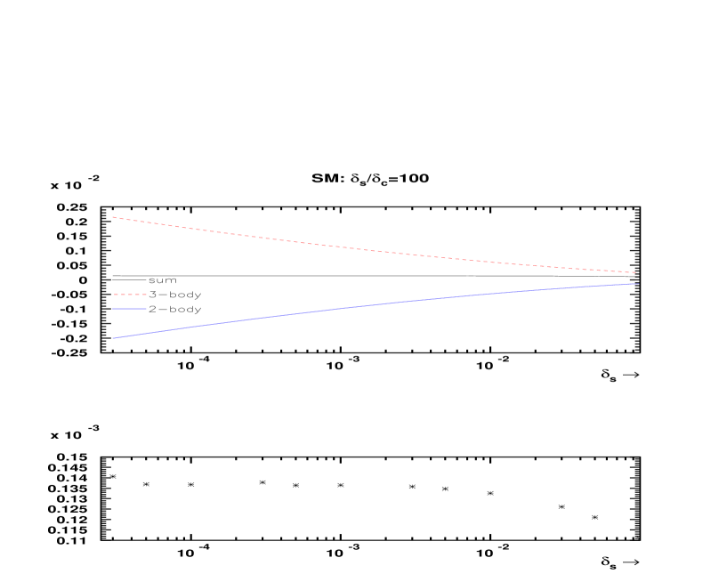
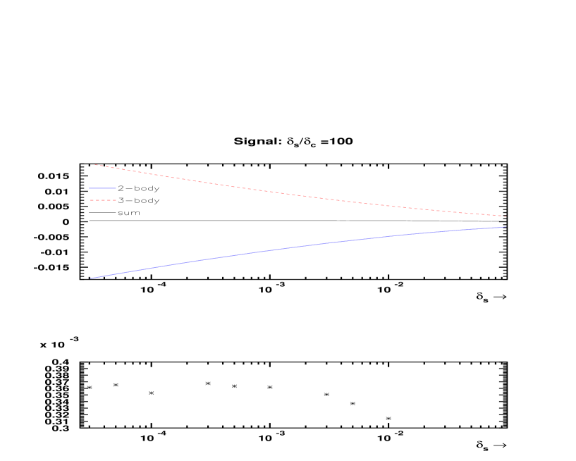
In the previous section we have given all the relevant analytical results, now we proceed to determine some kinematical distributions. First we demonstrate that the sum of 2-body and 3-body contributions is fairly independent of the slicing parameters. In Fig. 1 (for SM) and Fig. 2 (for signal) we show the variations of these two pieces with the slicing parameters in invariant mass, $Q=\sqrt{(p_{3}+p_{4})^{2}}$, distribution at a value of invariant mass equal to $800GeV$. Here both $\delta_{s}$ and $\delta_{c}$ are varied together with the ratio $\delta_{s}/\delta_{c}$ fixed at a value of 100 [16]. We note that the sum of 2-body and 3-body contributions is fairly stable against variations in these parameters and this gives us confidence in our code. In what follows we will use $\delta_{s}=10^{-3}$ and $\delta_{c}=10^{-5}$.

Below we present various distributions for the LHC with a center of mass energy of $14~{}TeV$ as a default choice. However we will also present some results for a center of mass energy of $10~{}TeV$ for the LHC. For numerical evaluation, the following SM parameters [25] are used

$$m=91.1876~{}GeV,\quad\sin^{2}\theta_{W}=0.231$$ (40)

where $\theta_{W}$ is the weak mixing angle. For the electromagnetic coupling constant $\alpha$ we use $\alpha^{-1}=128.89$. CTEQ6 [26, 27] density sets are used for parton distribution functions. 2-loop running for the strong coupling constant is used which is given by the expression,

$$a_{s}(\mu_{R}^{2})=\frac{1}{\beta_{0}\ln{\displaystyle\frac{\mu_{R}^{2}}{\Lambda_{QCD}^{2}}}}\left[1-\frac{(\beta_{1}/\beta_{0})~{}\ln\ln{\displaystyle\frac{\mu_{R}^{2}}{\Lambda_{QCD}^{2}}}}{\beta_{0}\ln{\displaystyle\frac{\mu_{R}^{2}}{\Lambda_{QCD}^{2}}}}\right].$$ (41)

with

$$\beta_{0} = \frac{11}{3}C_{A}-\frac{4}{3}n_{f}T_{f},$$

$$\beta_{1} = \frac{34}{3}C_{A}^{2}-\frac{4}{3}n_{f}T_{f}(3C_{F}+5C_{A}),$$ (42)

where the symbols are as given in Eq. 18 with number of colors equal to three. The number of active light-quark flavors is denoted by $n_{f}~{}(=5)$ and the value of $\Lambda_{QCD}$ is chosen as prescribed by the CTEQ6 density sets. At leading order, that is at order $a_{s}^{0}$, we use CTEQ6L1 density set ( which uses the LO running $a_{s}$ ) with the corresponding $\Lambda_{QCD}=165~{}MeV$. At NLO we use CTEQ6M density set ( which uses 2-loop running $a_{s}$ ) with the $\Lambda_{QCD}=226~{}MeV$; this value of $\Lambda_{QCD}$ enters into the evaluation of the 2-loop strong coupling. The default choice for the renormalization and factorization scale is the identification to the invariant mass of the $Z$ boson pair ie., $\mu_{F}=\mu_{R}=Q$. Furthermore the $Z$ bosons will be constrained to satisfy $|y_{Z}|<2.5$, where $y_{Z}$ is the rapidity of a final state $Z$ boson .

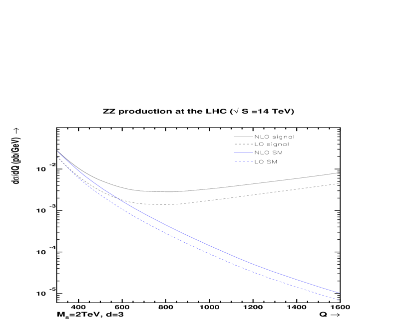
In Fig. 3 we have plotted the invariant mass distribution both for the SM and the signal, in the range 300 $GeV$ to 1600 $GeV$. The distribution is presented at the higher values of $Q$ as it is in this region the deviations from SM are more pronounced. In this plot we display for three extra dimensions ie., $d=3$, for fundamental scale equal to $2~{}TeV$. We see that for this choice of parameters the signal starts deviating significantly from the SM predictions around 400 $GeV$. To highlight the importance of QCD corrections we have also displayed the LO results of SM and the signal, and we observe that the $K$ factors (defined as $K=d\sigma^{NLO}/d\sigma^{LO}$) are large. For the signal the $K$ factor is 1.98 at $Q=600~{}GeV$ and 1.82 at $Q=1600~{}GeV$.

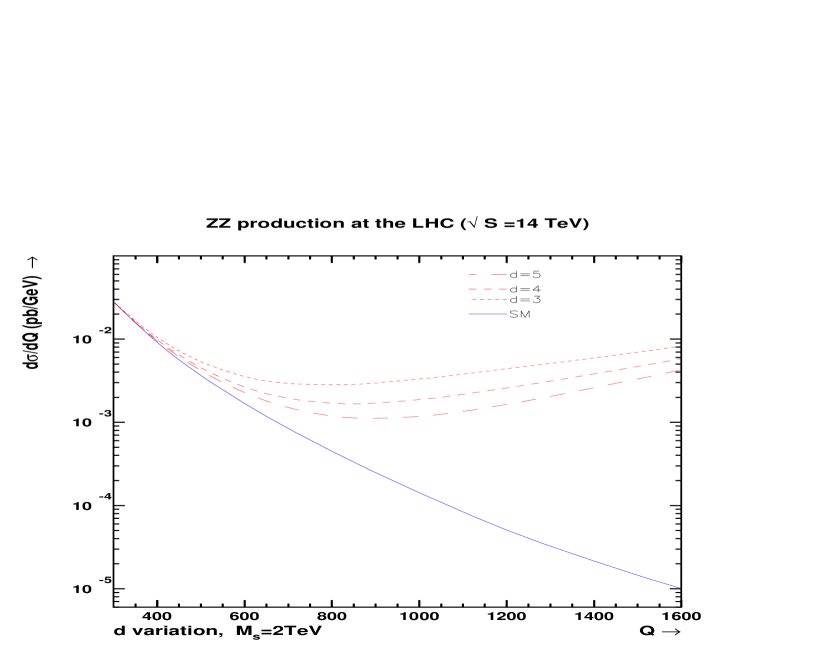
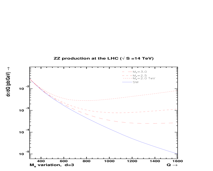
To estimate the effect of the number of extra dimension on the invariant mass distribution, we plot in Fig. 4 the signal for three different values of $d$ (3,4,5) with $M_{s}$ fixed at 2 $TeV$. We note that the lower the value of $d$ more is the strength of the signal. Next in Fig. 5 we have plotted $d\sigma/dQ$ for three different values of $M_{s}$ (2.0, 2.5, 3.0) at a fixed value 3 for the number of extra dimensions. As expected, with increase in the fundamental scale the deviations from SM predictions become less, and significant deviations from SM are observed at higher energies still.

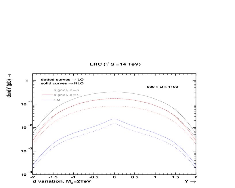
If Fig. 6 we have plotted the rapidity distribution $d\sigma/dY$ at LO and NLO both for SM and the signal for $d=3$ and $d=4$. The rapidity Y is defined as

$$Y=\frac{1}{2}\ln\frac{P_{1}\cdot q}{P_{2}\cdot q},$$ (43)

where $P_{1}$ and $P_{2}$ are incoming proton momenta and $q=p_{3}+p_{4}$ ie., sum of the $Z$ boson 4-momenta. We have plotted this distribution in the interval $-2.0<Y<2.0$ and have carried out an integration over the invariant mass interval $900<Q<1100$ to increase the signal over the SM background. As expected the distribution is symmetric about $Y=0$.

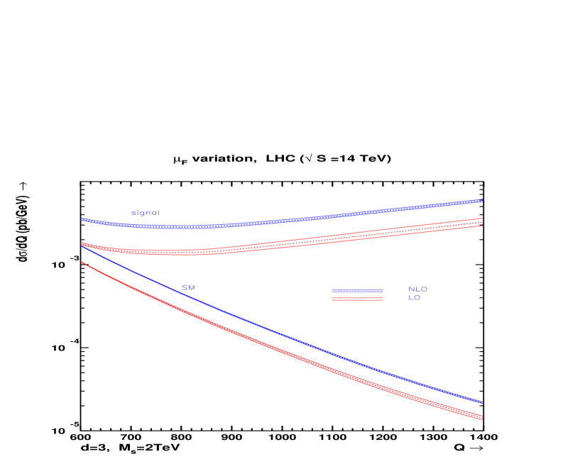
We have mentioned before that the NLO QCD corrections reduce the sensitivity of the cross sections to the factorization scale $\mu_{F}$; this we now show in the Fig. 7. We have plotted SM and the signal both at LO and NLO, and have varied the factorization scale $\mu_{F}$ in the range $Q/2<\mu_{F}<2Q$. The central curve in a given band (shown by the dotted curves) correspond to $\mu_{F}=Q$. In all these the renormalization scale is fixed at $\mu_{R}=Q$. We notice that the factorization scale uncertainties in SM are reduced compared to the signal. This is because of the dominant role of the gluon gluon initiated process in the signal. Most importantly we have been able to demonstrate that a significant reduction in factorization scale uncertainty is achieved by carrying out a full NLO computation. For instance at $Q=1400~{}GeV$ varying $\mu_{F}$ between $Q/2$ to $2Q$ shows a variation of $20.4\%$ at LO for the signal, however the NLO result at the same $Q$ value shows a variation of $6.4\%$.

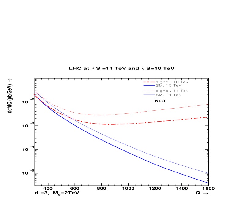
At the end we present in Fig. 8, $d\sigma/dQ$ for LHC with a centre of mass energy of $10~{}TeV$ at NLO both for SM and signal. For comparison we have also plotted the $14~{}TeV$ results in the same figure.

4 Summary and Conclusions

In this paper we have carried out a full NLO QCD calculation for the production of two $Z$ bosons at the LHC at $14TeV$ in the large extra dimension model of ADD. Here we take all order $a_{s}$ contributions, both in the SM and in the gravity mediated processes and their interferences, into account. We have presented all the leading order and one loop virtual matrix element squared for the process. The method of two cutoff phase space slicing, on which our monte carlo FORTRAN code is based, is very briefly discussed. After offering some checks on our monte carlo code we obtained invariant mass and rapidity distributions both at LO and NLO. We use CTEQ 6L1 and CTEQ 6M parton density sets for LO and NLO observables, respectively. Significant enhancements over the LO predictions are observed. The $K$ factors are found to be large in the invariant mass distribution; for instance the signal has a $K$ factor of 1.98 at $Q=600~{}GeV$ and 1.82 at $Q=1600~{}GeV$. We have also presented the effects of variation of number of extra dimensions $d$ and the fundamental scale $M_{s}$ in the $Q$ distribution. We have shown that a significant reduction in LO theoretical uncertainty, arising from the factorization scale, is achieved by our NLO computation. For instance at $Q=1400~{}GeV$ varying $\mu_{F}$ between $Q/2$ to $2Q$ shows a variation of $20.4\%$ at LO for the signal, however the NLO result at the same $Q$ value shows a variation of $6.4\%$. Thus our NLO results are more precise than the LO results and suitable for further studies for constraining the parameters of the ADD model. Invariant mass distribution is also presented for LHC at a center of mass energy of $10TeV$ at the NLO level.

Acknowledgments: The work of NA is supported by CSIR Senior Research Fellowship, New Delhi. NA, AT and VR would also like to thank the cluster computing facility at Harish-Chandra Research Institute. NA and VKT acknowledge the computational support of the computing facility which has been developed by the Nuclear Particle Physics Group of the Physics Department, Allahabad University under the Center of Advanced Study (CAS) funding of U.G.C. India. The authors would like to thank Prakash Mathews, Swapan Majhi and M.C. Kumar for useful discussions.

Figure 1: Variation of 2-body and 3-body contributions (of $d\sigma/dQ$ at $Q=800~{}GeV$ in SM) and their sum with $\delta_{s}$. Here $\delta_{s}/\delta_{c}=100$ has been used.

Figure 2: Variation of 2-body and 3-body contributions (of $d\sigma/dQ$ at $Q=800GeV$ in signal) and their sum with $\delta_{s}$. Here $\delta_{s}/\delta_{c}=100$ has been used.

Figure 3: Invariant mass distribution at LO and NLO in SM and for the signal at $M_{s}=2TeV$ and 3 extra dimensions.

Figure 4: Effect of variation of number of extra dimensions in invariant mass distribution. The fundamental scale $M_{s}$ has been fixed at 2 TeV. The curves correspond to NLO results.

Figure 5: Effect of variation of the fundamental scale $M_{s}$ in the invariant mass distribution. The number of extra dimensions has been fixed at 3. The curves correspond to NLO results.

Figure 6: Rapidity distribution for $M_{s}=2TeV$ for SM and signal for $d=3$ and $d=4$. The dotted curves correspond to the LO and solid curves to NLO. We have integrated over the invariant mass range $900<Q<1100$ to enhance the signal.

Figure 7: Factorization scale variation in the invariant mass distribution. The number of extra dimensions $d=3$ and the fundamental scale $M_{s}=2TeV$ have been chosen. LO curves correspond to CTEQ 6L1 density sets and NLO curves to CTEQ 6M sets.

Figure 8: Invariant mass distribution at NLO for SM and the signal. Here the thicker curves correspond to $\sqrt{S}=10TeV$ and lighter curves to $\sqrt{S}=14TeV$ at the LHC.

5 Appendix

$$\overline{|M^{V}|^{2}}^{fin}_{q\overline{q},sm} = {e^{4}\over N}\left(C_{v}^{4}+6~{}C_{v}^{2}C_{a}^{2}+C_{a}^{4}\right){\cal T}_{W}^{4}~{}\left(\frac{1}{8t^{2}u^{2}}\right)$$ (44)

$$\times\Bigg{[}\Bigg{\{}\frac{u~{}F_{1}(t)}{(t-m^{2})^{2}}\Big{(}3m^{8}(-4t+u)+6m^{6}t(2t+u)-2m^{2}t^{2}u(4t+u)$$

$$+t^{3}u(2t+3u)+m^{4}t(-2t^{2}+tu-3u^{2})\Big{)}$$

$$+u~{}F_{2}(t)\Big{(}m^{4}(8t-2u)-4m^{2}t(2t+u)+t(2t^{2}+2tu+u^{2})\Big{)}+t\leftrightarrow u\Bigg{\}}$$

$$+2\zeta(2)\Big{(}-20m^{2}tu(t+u)-4m^{4}(t^{2}-8tu+u^{2})+tu(5t^{2}+4tu+5u^{2})\Big{)}$$

$$+\frac{F_{3}}{(4m^{2}-s)^{2}}\Big{(}8m^{2}t^{2}u^{2}(t+u)+12m^{8}(t^{2}-8tu+u^{2})$$

$$-tu(t+u)^{2}(3t^{2}+4tu+3u^{2})+4m^{6}(3t^{3}-5t^{2}u-5tu^{2}+3u^{3})$$

$$+m^{4}(3t^{4}+14t^{3}u+78t^{2}u^{2}+14tu^{3}+3u^{4})\Big{)}$$

$$+~{}\frac{tu~{}F_{4}}{s(4m^{2}-s)^{2}}\Big{(}-32m^{6}tu-64m^{8}(t+u)+8m^{2}tu(t+u)^{2}$$

$$-(t+u)^{3}(3t^{2}+4tu+3u^{2})+m^{4}(22t^{3}+82t^{2}u+82tu^{2}+22u^{3})\Big{)}$$

$$+\frac{1}{(t-m^{2})(u-m^{2})(4m^{2}-s)}\Big{(}18m^{10}(t^{2}-8tu+u^{2})$$

$$+m^{8}(-9t^{3}+131t^{2}u+131tu^{2}-9u^{3})-7t^{2}u^{2}(t^{3}+t^{2}u+tu^{2}+u^{3})$$

$$-4m^{4}tu(4t^{3}+23t^{2}u+23tu^{2}+4u^{3})+m^{6}(-9t^{4}+14t^{3}u-66t^{2}u^{2}$$

$$+14tu^{3}-9u^{4})+m^{2}tu(9t^{4}+32t^{3}u+82t^{2}u^{2}+32tu^{3}+9u^{4})\Big{)}\Bigg{]}$$

$$\!\!\!\!\overline{|M^{V}|^{2}}^{fin}_{q\overline{q},int} = {e^{2}\kappa^{2}\over 8N}\left(C_{v}^{2}+C_{a}^{2}\right){\cal T}_{W}^{2}$$

$$\times\Bigg{[}\Big{\{}\frac{G_{1}(t)}{t\left(m^{2}-t\right)}\Big{(}-9m^{8}-4m^{4}t^{2}+3m^{6}(5t+u)-m^{2}tu(9t+u)$$

$$+t^{2}u(2t+3u)\Big{)}+\frac{G_{2}(t)}{t}\Big{(}6m^{6}-2m^{4}(8t+u)+m^{2}t(10t+7u)$$

$$-t(2t^{2}+2tu+u^{2})\Big{)}+t\leftrightarrow u\Big{\}}-\frac{2G_{3}}{tu}\Big{(}-18m^{6}(t+u)$$

$$-37m^{2}tu(t+u)+m^{4}(6t^{2}+80tu+6u^{2})+tu(7t^{2}+4tu+7u^{2})\Big{)}$$

$$+\frac{G_{4}}{tu\left(u-m^{2}\right)\left(m^{2}-t\right)}\Big{(}9m^{10}(t+u)+m^{4}tu(t^{2}+10tu+u^{2})$$

$$-6m^{8}\left(2t^{2}+5tu+2u^{2}\right)+t^{2}u^{2}(3t^{2}+4tu+3u^{2})$$

$$-m^{2}tu(t^{3}+14t^{2}u+14tu^{2}+u^{3})+m^{6}(3t^{3}+19t^{2}u+19tu^{2}+3u^{3})\Big{)}$$

$$-\frac{G_{5}}{s\left(4m^{2}-s\right)^{2}}\Big{(}-128m^{10}+48m^{8}(t+u)+48m^{6}(t^{2}+3tu+u^{2})$$

$$+(t+u)^{3}(3t^{2}+4tu+3u^{2})-m^{2}(t+u)^{2}(5t^{2}+18tu+5u^{2})$$

$$-2m^{4}(7t^{3}+37t^{2}u+37tu^{2}+7u^{3})\Big{)}+\frac{G_{6}}{tu\left(4m^{2}-s\right)}\Big{(}-114m^{8}(t+u)$$

$$+m^{6}(-19t^{2}+334tu-19u^{2})-m^{2}tu(53t^{2}+190tu+53u^{2})$$

$$+17tu(t^{3}+t^{2}u+tu^{2}+u^{3})+m^{4}(19t^{3}+61t^{2}u+61tu^{2}+19u^{3})\Big{)}$$

$$+\frac{G_{7}}{tu\left(4m^{2}-s\right)^{2}}\Big{(}-36m^{10}(t+u)-8m^{8}(3t^{2}-13tu+3u^{2})$$

$$+tu(t+u)^{2}(3t^{2}+4tu+3u^{2})+m^{6}(3t^{3}+61t^{2}u+61tu^{2}+3u^{3})$$

$$+m^{4}(3t^{4}-2t^{3}u-98t^{2}u^{2}-2tu^{3}+3u^{4})-7m^{2}tu(t+u)^{3}\Big{)}\Bigg{]}$$

where

$$F_{1} = \displaystyle{\ln{-\frac{t}{m^{2}}}}~{},\quad\quad\quad\quad F_{2}=2\ln\left(-\frac{t}{m^{2}}\right)\ln\left\{\frac{(t-m^{2})^{2}}{m^{2}s}\right\}+4Li_{2}\left(\frac{t}{m^{2}}\right)-\ln^{2}\left(\frac{-t}{m^{2}}\right)~{},$$

$$F_{3} = \ln{\frac{s}{m^{2}}}~{},~{}~{}\quad\quad\quad\quad F_{4}=\frac{1}{\beta}\Big{[}\ln^{2}(\gamma)+4Li_{2}(-\gamma)+2\zeta(2)\Big{]}~{},~{}~{}$$

$$\gamma = \frac{1-\beta}{1+\beta}~{},\quad\quad\quad\quad\beta=\sqrt{1-4m^{2}/s}.$$ (46)

and

$$G_{1} = {\cal R}e{\cal D}_{s}\ln\left(\frac{-t}{m^{2}}\right),$$

$$G_{2} = 4{\cal R}e{\cal D}_{s}Li_{2}{\left(\frac{t}{m^{2}}\right)}+2{\cal R}e{\cal D}_{s}\ln{\left(\frac{-t}{m^{2}}\right)}\ln{\left(\frac{(m^{2}-t)^{2}}{m^{2}s}\right)}$$

$$+2{\cal I}m{\cal D}_{s}\pi\ln{\left(\frac{(m^{2}-t)^{2}}{m^{2}s}\right)}-{\cal R}e{\cal D}_{s}\ln{\left(\frac{-t}{m^{2}}\right)^{2}}-2{\cal I}m{\cal D}_{s}\pi\ln{\left(\frac{-t}{m^{2}}\right)},$$

$$G_{3} = \zeta(2){\cal R}e{\cal D}_{s},\quad\quad\quad\quad G_{4}={\cal I}m{\cal D}_{s}\pi,$$

$$G_{5} = \frac{{\cal R}e{\cal D}_{s}}{\beta}\ln^{2}{\left(\gamma\right)}+\frac{4}{\beta}{\cal R}e{\cal D}_{s}Li_{2}{\left(-\gamma\right)}+\frac{2{\cal R}e{\cal D}_{s}}{\beta}\zeta(2),$$

$$G_{6} = {\cal R}e{\cal D}_{s},\quad\quad\quad\quad G_{7}={\cal R}e{\cal D}_{s}\ln\left(s/m^{2}\right).$$ (47)

$$\!\!\!\!\overline{|M^{V}|^{2}}_{gg,int}^{fin} = \left(C_{v}^{2}+C_{a}^{2}\right){\cal T}_{W}^{2}\frac{1}{C_{A}}\frac{e^{2}\kappa^{2}}{N^{2}-1}$$ (48)

$$\times\Bigg{[}\Big{\{}H_{1}(t)\Big{(}9m^{4}+2t^{2}+2tu+u^{2}-6m^{2}(t+u)\Big{)}+\frac{H_{2}(t)}{4(t-m^{2})^{2}}\Big{(}-9m^{8}$$

$$+t^{2}u(2t+u)-2m^{2}tu(3t+u)+2m^{6}(5t+3u)-m^{4}(3t^{2}-2tu+u^{2})\Big{)}$$

$$+u\leftrightarrow t\Big{\}}+\frac{H_{3}}{4}\Big{(}18m^{4}+3t^{2}+4tu+3u^{2}-12m^{2}(t+u)\Big{)}$$

$$+\frac{H_{4}}{4(4m^{2}-s)^{2}}\Big{(}-32m^{8}+4m^{6}(t+u)-(t+u)^{2}(t^{2}+4tu+u^{2})$$

$$+m^{4}(6t^{2}+44tu+6u^{2})+2m^{2}(t^{3}-3t^{2}u-3tu^{2}+u^{3})\Big{)}+\frac{H_{5}}{s(4m^{2}-s)^{2}}\Big{(}80m^{10}$$

$$-32m^{8}(t+u)+8m^{2}tu(t+u)^{2}-16m^{6}(t^{2}+5tu+u^{2})$$

$$-(t+u)^{3}(3t^{2}+4tu+3u^{2})+2m^{4}(5t^{3}+31t^{2}u+31tu^{2}+5u^{3})\Big{)}$$

$$-\frac{H_{6}}{4(t-m^{2})^{2}(u-m^{2})^{2}}\Big{(}18m^{12}-34m^{10}(t+u)-t^{2}u^{2}(t^{2}+4tu+u^{2})$$

$$+m^{8}(25t^{2}+36tu+25u^{2})+2m^{2}tu(t^{3}+6t^{2}u+6tu^{2}+u^{3})$$

$$-4m^{6}(2t^{3}+t^{2}u+tu^{2}+2u^{3})+m^{4}(t^{4}-8t^{3}u-20t^{2}u^{2}-8tu^{3}+u^{4})\Big{)}$$

$$+\frac{H_{7}}{4(t-m^{2})(u-m^{2})(4m^{2}-s)}\Big{(}-28m^{10}+8m^{6}tu+26m^{8}(t+u)$$

$$+tu(t^{3}+t^{2}u+tu^{2}+u^{3})-m^{4}(5t^{3}+23t^{2}u+23tu^{2}+5u^{3})$$

$$+m^{2}(t^{4}+4t^{3}u+10t^{2}u^{2}+4tu^{3}+u^{4})\Big{)}\Bigg{]}$$

where

$$H_{1}(t) = \frac{1}{8}\Bigg{(}2{\cal R}e{\cal D}_{s}\ln\left(\frac{-t}{m^{2}}\right)\ln\left(\frac{(m^{2}-t)^{2}}{m^{2}s}\right)$$ (49)

$$+2{\cal I}m{\cal D}_{s}\pi\ln\left(\frac{(m^{2}-t)^{2}}{m^{2}s}\right)+4{\cal R}e{\cal D}_{s}Li_{2}{\left(\frac{t}{m^{2}}\right)}$$

$$-{\cal R}e{\cal D}_{s}\ln\left(\frac{-t}{m^{2}}\right)^{2}-2{\cal I}m{\cal D}_{s}\pi\ln\left(\frac{-t}{m^{2}}\right)\Bigg{)},$$

$$H_{1}(u) = \frac{1}{8}\Bigg{(}2{\cal R}e{\cal D}_{s}\ln\left(\frac{-u}{m^{2}}\right)\ln\left(\frac{(m^{2}-u)^{2}}{m^{2}s}\right)$$ (50)

$$+2{\cal I}m{\cal D}_{s}\pi\ln\left(\frac{(m^{2}-u)^{2}}{m^{2}s}\right)+4{\cal R}e{\cal D}_{s}Li_{2}{\left(\frac{u}{m^{2}}\right)}$$

$$-{\cal R}e{\cal D}_{s}\ln\left(\frac{-u}{m^{2}}\right)^{2}-2{\cal I}m{\cal D}_{s}\pi\ln\left(\frac{-u}{m^{2}}\right)\Bigg{)},$$

$$H_{2}(t) = {\cal R}e{\cal D}_{s}\ln\left(\frac{-t}{m^{2}}\right),\quad\quad\quad\quad H_{2}(u)={\cal R}e{\cal D}_{s}\ln\left(\frac{-u}{m^{2}}\right),$$

$$H_{3} = \zeta(2){\cal R}e{\cal D}_{s},\quad\quad\quad\quad H_{4}={\cal R}e{\cal D}_{s}ln\left(\frac{s}{m^{2}}\right),$$

$$H_{5} = \frac{1}{8}\Big{(}\frac{{\cal R}e{\cal D}_{s}}{\beta}\ln^{2}{\left(\gamma\right)}+\frac{4}{\beta}{\cal R}e{\cal D}_{s}Li_{2}{\left(-\gamma\right)}+\frac{2{\cal R}e{\cal D}_{s}}{\beta}\zeta(2)\Big{)},$$

$$H_{6} = {\cal I}m{\cal D}_{s}\pi,\quad\quad\quad\quad H_{7}={\cal R}e{\cal D}_{s}.$$

\begin{picture}(200.0,40.0) \put(0.0,0.0){} \put(0.0,0.0){} \put(0.0,0.0){} \put(0.0,0.0){} \put(0.0,0.0){} \end{picture}

Figure 9: Leading order diagram in SM. The diagram with the momenta of final state $Z$ bosons interchanged (which is not shown here) also contributes.

Figure 10: Order $a_{s}$ virtual diagrams in SM. The diagrams with the momenta of final state $Z$ bosons interchanged (which are not shown here) also contribute.

Figure 11: Order $a_{s}$ real emission Feynman diagrams in SM. The diagrams with the momenta of final state $Z$ bosons interchanged (which are not shown here) also contribute.

Figure 12: LO gravity mediated diagrams.

Figure 13: Order $a_{s}$ gravity mediated virtual correction Feynman diagrams.

Figure 14: Gravity mediated real emission diagrams which contribute at NLO.

References

- [1] I. Antoniadis, N. Arkani-Hamed, S. Dimopoulos and G. R. Dvali, Phys. Lett. B 436, 257 (1998) [arXiv:hep-ph/9804398].
- [2] N. Arkani-Hamed, S. Dimopoulos and G. R. Dvali, Phys. Lett. B 429, 263 (1998) [arXiv:hep-ph/9803315].
- [3] K. Hagiwara, R. D. Peccei, D. Zeppenfeld and K. Hikasa, Nucl. Phys. B 282 (1987) 253.
- [4] R. W. Brown and K. O. Mikaelian, Phys. Rev. D 19 (1979) 922.
- [5] U. Baur, E. W. N. Glover and J. J. van der Bij, Nucl. Phys. B 318 (1989) 106.
- [6] M. Kober, B. Koch and M. Bleicher, Phys. Rev. D 76, 125001 (2007) [arXiv:0708.2368 [hep-ph]].
- [7] J. Gao, C. S. Li, X. Gao and J. J. Zhang, Phys. Rev. D 80, 016008 (2009) [arXiv:0903.2551 [hep-ph]].
- [8] J. Ohnemus and J. F. Owens, Phys. Rev. D 43, 3626 (1991).
- [9] B. Mele, P. Nason and G. Ridolfi, Nucl. Phys. B 357, 409 (1991).
- [10] L. J. Dixon, Z. Kunszt and A. Signer, Phys. Rev. D 60, 114037 (1999) [arXiv:hep-ph/9907305].
- [11] J. M. Campbell and R. K. Ellis, Phys. Rev. D 60, 113006 (1999) [arXiv:hep-ph/9905386].
- [12] M. C. Kumar, P. Mathews, V. Ravindran and A. Tripathi, Phys. Lett. B 672, 45 (2009) [arXiv:0811.1670 [hep-ph]].
- [13] M. C. Kumar, P. Mathews, V. Ravindran and A. Tripathi, Nucl. Phys. B 818, 28 (2009) [arXiv:0902.4894 [hep-ph]].
- [14] P. Mathews, V. Ravindran, K. Sridhar and W. L. van Neerven, Nucl. Phys. B 713, 333 (2005) [arXiv:hep-ph/0411018].
- [15] M. C. Kumar, P. Mathews and V. Ravindran, Eur. Phys. J. C 49, 599 (2007) [arXiv:hep-ph/0604135].
- [16] B. W. Harris and J. F. Owens, Phys. Rev. D 65, 094032 (2002) [arXiv:hep-ph/0102128].
- [17] J. A. M. Vermaseren, arXiv:math-ph/0010025.
- [18] G. ’t Hooft and M. J. G. Veltman, Nucl. Phys. B 44 (1972) 189;
- [19] P.Breitenlohner, B. Maison, Commun.Math.53 (1977) 11, P.Breitenlohner, B. Maison, Commun.Math.53 (1977) 39, P.Breitenlohner, B. Maison, Commun.Math.53 (1977) 55.
- [20] G. F. Giudice, R. Rattazzi and J. D. Wells, Nucl. Phys. B 544 (1999) 3 [arXiv:hep-ph/9811291].
- [21] T. Han, J. D. Lykken and R. J. Zhang, Phys. Rev. D 59 (1999) 105006 [arXiv:hep-ph/9811350].
- [22] G. Passarino and M. J. G. Veltman, Nucl. Phys. B 160, 151 (1979).
- [23] G. Duplancic and B. Nizic, Eur. Phys. J. C 20, 357 (2001) [arXiv:hep-ph/0006249].
- [24] Z. Bern, L. J. Dixon and D. A. Kosower, Nucl. Phys. B 412, 751 (1994) [arXiv:hep-ph/9306240].
- [25] C. Amsler et al. [Particle Data Group], Phys. Lett. B 667, 1 (2008).
- [26] J. Pumplin, D. R. Stump, J. Huston, H. L. Lai, P. M. Nadolsky and W. K. Tung, JHEP 0207 (2002) 012 [arXiv:hep-ph/0201195].
- [27] D. Stump, J. Huston, J. Pumplin, W. K. Tung, H. L. Lai, S. Kuhlmann and J. F. Owens, JHEP 0310 (2003) 046 [arXiv:hep-ph/0303013].