Dark Energy Properties in DBI Theory

Abstract

The Dirac-Born-Infeld (DBI) action from string theory provides several new classes of dark energy behavior beyond quintessence due to its relativistic kinematics. We constrain parameters of natural potentials and brane tensions with cosmological observations as well as showing how to design these functions for a desired expansion history. We enlarge the attractor solutions, including new ways of obtaining cosmological constant behavior, to the case of generalized DBI theory with multiple branes. An interesting novel signature of DBI attractors is that the sound speed is driven to zero, unlike for quintessence where it is the speed of light.

I Introduction

High energy physics theories for dark energy causing the accelerated expansion of the universe face issues of naturalness – why is the current dark energy density measured so different from the initial conditions of the high energy, early universe, and how is the current low energy form of the potential energy related to the initial high energy form that should receive quantum corrections?

The cosmological constant in particular suffers both problems. Making the field dynamical helps. To more fully solve the amplitude problem one would like an attractor solution, where the present behavior is largely insensitive to the exact initial conditions. To ameliorate the form problem one would like a symmetry or geometric quantity that protects the potential, or ideally have it predicted from a fundamental theory such as string theory. Quintessence models cannot achieve both properties, and even the attractor solutions have difficulty in naturally reaching a dark energy equation of state $w\approx-1$ zws as indicated by cosmological observations.

Paper 1 akl , following the pioneering paper of martinyam , highlighted the DBI class from string theory as possessing desirable properties to serve as dark energy. In particular, it found not only the attractor solutions accessible to quintessence, but three new classes that could achieve or approach $w=-1$, the cosmological constant state. String theory can impose a specific non-trivial kinetic behavior through the Dirac-Born-Infeld (DBI) action that arises naturally in consideration of D3-brane motion within a warped compactification. The field properties are related to the geometric position of a three dimensional brane within higher dimensions, and the brane tension and potential functions are (in principle) given by string theory, in particular through the AdS/CFT correspondence.

In this paper we extend the attractor solutions as well as more fully considering the entire evolution and its observational consequences. In §II we examine in detail the case motivated by the simplest physics and find the viable regions of parameter space constrained through cosmological observations. We show in §III how to construct the required potential for a given cosmic expansion history or equation of state. Generalizing DBI theory to multiple branes or non-standard branes adds a degree of freedom which we analyze in §IV. We explore a new window on constraining DBI dark energy with observations in terms of the dark energy sound speed – this gives a distinct prediction from quintessence – and its effects on the matter density power spectrum in §V.

II Constraints on a Natural DBI Model

The DBI action arises in Type IIB string theory in terms of the volume swept out by a D3-brane in a warped geometry, coupled to gravity. The form is

$$S=\int d^{4}x\,\sqrt{-g}\,\left[-T(\phi)\sqrt{1-\dot{\phi}^{2}/T(\phi)}+T(\phi)-V(\phi)\right],$$ (1)

where we ignore the spatial derivatives of $\phi$. $T$ is the warped brane tension and $V$ is the potential arising from interactions with Ramond-Ramond fluxes or other sectors. See, e.g., siltong for more details. The kinetic factor is often written in terms of a Lorentz boost factor

$$\gamma\equiv\frac{1}{\sqrt{1-\dot{\phi}^{2}/T}}\,,$$ (2)

and the DBI dark energy equation of state is

$$w\equiv\frac{p_{\phi}}{\rho_{\phi}}=-\frac{\gamma^{-1}-1+v}{\gamma-1+v}\,,$$ (3)

where $v=V/T$. The nonrelativistic limit $\gamma-1\ll 1$ leads to the quintessence action and equation of state.

In akl the main consideration was the critical points of the equations of motion and the asymptotic attractor behavior. In this section we consider perhaps the most natural forms for the tension and potential and follow the specific dynamics throughout the history of the universe. A complete string theory would predict the functions $T$ and $V$; while this is not available one can use known behaviors for certain circumstances. For a pure AdS₅ geometry with radius $R$, the warped tension is given by

$$T(\phi)=\tau\,\phi^{4}\,,$$ (4)

with $\tau=1/(g_{s}\tilde{\lambda})$ where $g_{s}$ is the string coupling, $\alpha^{\prime}$ is the inverse string tension, and $\tilde{\lambda}=R^{4}/\alpha^{\prime 2}$ which is identified as the ’t Hooft coupling in AdS/CFT correspondence.

The potential is expected to have quadratic terms arising from the breaking of conformal invariance due to couplings to gravity and other sectors. In addition, quartic terms enter from such interactions, while higher order terms are suppressed, e.g. by powers of $1/R$ siltong ; ast . We therefore take an ansatz

$$V(\phi)=m^{2}\phi^{2}+cT=m^{2}\phi^{2}+c\tau\phi^{4}\,.$$ (5)

Note that we take the potential to have a true zero minimum so that there is no intrinsic cosmological constant.

For reference, we briefly review the equation of motion. The DBI version of the Klein-Gordon equation is

$$\ddot{\phi}+3\gamma^{-2}H\dot{\phi}+\gamma^{-3}V_{,\phi}+\frac{1}{2}(3\gamma^{-2}-2\gamma^{-3}-1)\,T_{,\phi}=0\,,$$ (6)

where $H$ is the Hubble parameter, $V_{,\phi}=dV/d\phi$ and $T_{,\phi}=dT/d\phi$. The energy-momentum tensor has perfect fluid form with energy density $\rho_{\phi}$ and pressure $p_{\phi}$ given by

$$\rho_{\phi}=(\gamma-1)\,T+V\quad;\quad p_{\phi}=(1-\gamma^{-1})\,T-V\,,$$ (7)

and so the equation of motion can also be viewed in terms of the continuity equation

$$\dot{\rho}_{\phi}=-3H(\rho_{\phi}+p_{\phi})=-3H(\gamma-\gamma^{-1})\,T\,.$$ (8)

For the form of Eq. (5), the potential for large $\phi$ is dominated by the quartic term while for small $\phi$ it looks like a quadratic potential. akl identified the ratio $V/T$ as particularly important for determining the attractor, if any. With Eq. (4) this implies that

$$v\equiv\frac{V}{T}=c+\mu^{2}\,(\kappa\phi)^{-2}\,$$ (9)

where $\mu^{2}=(m^{2}\kappa^{2}/\tau)$ and $\kappa^{2}=8\pi G$. At late times, $\phi$ rolls to zero and the quantity $v$ is dominated by the second term in Eq. (9) so $v\to\infty$, giving the ultrarelativistic class of attractor solutions discussed by akl . In particular, since $\lambda\equiv-(1/\kappa V)dV/d\phi\sim 1/\phi$ and $\gamma\sim v\sim\phi^{-2}$ in this limit, then the secondary attractor parameter of akl is $\lambda^{2}/\gamma=$ const. This implies that it is the second class of attractor solution from Table I of akl that is reached and at late times $w=-1+\lambda^{2}/(3\gamma)$. However the evolution at present and at all times before the asymptotic future is of interest.

Figure 1 illustrates the dynamical evolution of these models in the $w$-$w^{\prime}$ plane, where $w^{\prime}=dw/d\ln a$, for various values of $c$ and $\mu^{2}$. The most noticeable common characteristic of the field evolution is that it is a thawing field. That is, the dynamical history lies within the thawing region of the $w$-$w^{\prime}$ phase plane defined originally for quintessence as bounded by $1\leq w^{\prime}/(1+w)\leq 3$, as one of the two major classes of evolution caldwelllinder . Indeed, the field evolves away from a frozen, $w=-1$ state in the high redshift, matter dominated era along the $w^{\prime}=3(1+w)$ line defined by caldwelllinder and shown to be a generic dynamical flow solution by cahndl . The evolution remains within the thawing region, until today (defined by $\Omega_{\phi}=0.72$ and denoted by an x along the evolutionary track) the field lies roughly near $w^{\prime}\approx(1+w)$.

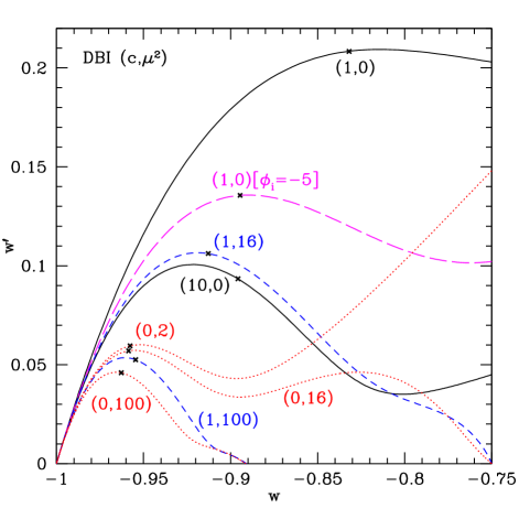
Figure 1: The DBI solutions using quartic/quadratic potential/tension functions of Eq. (9) are plotted in the $w$-$w^{\prime}$ plane. The initial thawing behavior, the values today (denoted by x’s along the curves) with property $w^{\prime}\approx 1+w$, and future attractors to a constant $w$ determined by the value of $\mu^{2}$ are all evident.

At early times, in the matter dominated era, the field is frozen to a cosmological constant state, until the DBI dark energy density become nonnegligible. This is independent of initial field value $\phi_{i}$ and velocity $\gamma_{i}$, as Fig. 2 illustrates. The freezing represents the effects of matter domination and is a different sort of attractor than the late time solution. The thawing occurs in a manner that does depend on $\phi_{i}$, but is insensitive today to $\phi_{i}$ for $|\phi_{i}|<1$. In the future, the DBI attractor ensures the same solution regardless of $\phi_{i}$.

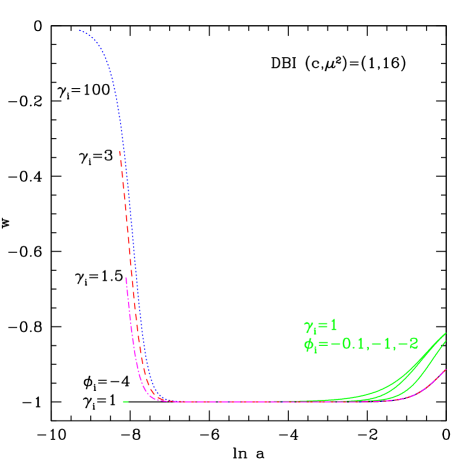
Figure 2: The high Hubble friction during matter domination freezes the field to $w=-1$ for many e-folds in expansion, despite an initial field velocity measured in terms of the Lorentz factor $\gamma_{i}$. This pseudo-attractor ensures that models with different $\gamma_{i}$ then follow the same trajectory, as shown by the convergence of tracks from the left side (early times) to the middle (later times). (Tracks start in the plot at $\Omega_{\phi}=10^{-10}$, with $\phi_{i}=-4$ and the $\gamma_{i}$ as labeled.) The light, green curves diverging from the middle to the right side (today) show this is not a true attractor since the thawing rate does depend on the initial field value $\phi_{i}$ (here fixing $\gamma_{i}=1$). However, the late time, true attractor from DBI dynamics will bring all these trajectories together; indeed at present all models with $\kappa\phi_{i}<1$ have the same dynamics.

At late times the field only notices the quadratic part of the potential; that is, this attractor solution only requires that the potential look quadratic near the minimum – a highly generic state. The evolution of the field up to the present, however, does depend on the quartic term: contrast the $(c,\mu^{2})=(0,16)$ and $(1,16)$ curves in Fig. 1. At all times until the final asymptotic value the specific evolution differs, in particular up to the present.

These differences allow us to constrain the parameters of the theory by comparing to cosmological observations. Here we consider the distance-redshift relation over the range $z=0-1.7$, as given by Type Ia supernovae. We examine the maximum fractional difference $\delta d/d_{\Lambda}$ of the model predictions for distances from those of the flat, cosmological constant plus matter universe with $\Omega_{\Lambda}=1-\Omega_{m}=0.72$.

One question we can ask is what are the bounds on $\mu^{2}$ such that the distance deviation is less than some value, say 2%. Large values of $\phi_{i}$ give a lengthy frozen state (note $(1/V)[dV/d(\kappa\phi)]\sim 1/\phi$ becomes small), lasting until close to the present, so $w\approx-1$. This will give little deviation from a cosmological constant so the most stringent bounds on $\mu^{2}$ occur for small $\phi_{i}$. For $\kappa\phi_{i}\lesssim 1$, though, the potential tends to be dominated by the quadratic, attractor part and the field quickly forgets the initial value (compare the $\kappa\phi_{i}=-0.1$ vs. $\kappa\phi_{i}=-1$ curves in Fig. 2). This also makes the bound fairly insensitive to the value of $c$. A fitting formula to the constraint on $\mu$ is

$$\mu>7.1\,(1+0.002c)\left(\frac{\delta d/d_{\Lambda}}{2\%}\right)^{-1}\,.$$ (10)

Note the weak dependence on $c$. The inverse proportionality to $\delta d/d_{\Lambda}$, for small deviations, arises from the maximum deviation in the equation of state $1+w$. The attractor value is given by akl

$$1+w_{c}=\frac{2}{3\mu^{2}}\left[-1+\sqrt{1+3\mu^{2}}\right]\,,$$ (11)

which is inversely proportional to $\mu$, for $\mu^{2}\gg 1$.

While Eq. (10) gives the most stringent bound to agree with observations, models with lesser values of $\mu$ are viable if the values of $\phi_{i}$ are large enough. Figure 3 show the constraints in the $c$-$\phi_{i}$ plane for a maximum allowed distance deviation of 2%. For $\mu^{2}\gtrsim 55$, the distance deviation is less than 2% for all cases with $c<20$. The maximum tends to be quite shallow: for $\mu^{2}=50$ most of the disallowed lower half plane actually has $0.02<\delta d/d<0.021$. The largest deviation for $\mu^{2}=50$ (40) occurs for $c=20$ and is at the 2.18% (2.44%) level. The figure exemplifies how cosmological observations can directly inform us on string theory parameters.

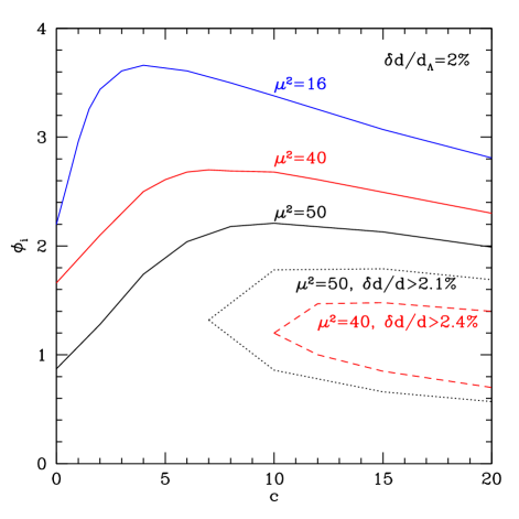
Figure 3: Model parameters can be constrained by comparison to distance data, here taken to be within 2% of $\Lambda$CDM. Above the solid curves for each value of $\mu^{2}$ the deviation is less than 2% (as $\phi_{i}$ gets large, $w$ has deviated less from the value $w=-1$ imposed by the matter dominated freezing). Below the solid curves the distance deviation is larger, but often by a small amount: only within the dotted, black contour is the deviation more than 2.1% for $\mu^{2}=50$, and similarly the dashed, red contour bounds the deviation to 2.4% for $\mu^{2}=40$.

III Customized Expansion History

From Eq. (3), we can write down a solution for the form of the potential for any expansion history desired, i.e. any given equation of state evolution $w(a)$ (including $w$ constant). The reduced potential, $v=V(\phi)/T(\phi)$ must satisfy

$$v(a)=1-\frac{w(a)\,\gamma(a)}{1+w(a)}-\frac{\gamma(a)^{-1}}{1+w(a)}\,.$$ (12)

Note this expression holds even for a time dependent $\gamma$ (we are here interested in the full evolution, not just the attractor state). Combining this expression for $v(a)$ with the solutions of the equations of motion for $\gamma(a)$ and $\phi(a)$, one can construct the potential $V(\phi)$ for any desired equation of state function.

Figure 4 shows the potential $V(\phi)$ constructed (taking $T\sim\phi^{4}$) to give constant $w$ for all times, for the cases $w=-0.99$, $-0.9$, and $-0.8$. (If $w=-1$ exactly then the field does not roll at all and the potential cannot be reconstructed.) The conditions for $w\approx-1$ to be realized (for constant $w$) can be written through Eq. (3) in terms of the initial values (note we are not describing an attractor solution) and are that either $v_{i}\gg\gamma_{i}$ or $v_{i}\gg\gamma_{i}-1$. For $\gamma_{i}=1+\epsilon$, with $\epsilon$ a small quantity, $w\approx-1+2\epsilon/v_{i}$ if the second condition holds. When the first condition holds, $w\approx-1+[(\gamma_{i}^{2}-1)/\gamma_{i}](1/v_{i})$. In either case, $w\to-1$. The potential is steep initially (roughly $\lambda^{2}\sim\Omega_{\phi,i}^{-1}$) and the field rolls to $\phi=0$. The shape of the potential near $\phi=0$ is given by $V(\phi\ll 1)\sim\phi^{2}$ (since we took $T\sim\phi^{4}$), as required by our previous results. However, as noted there, the potential when the dynamics is off the attractor trajectory does not need to stay in the asymptotic form.

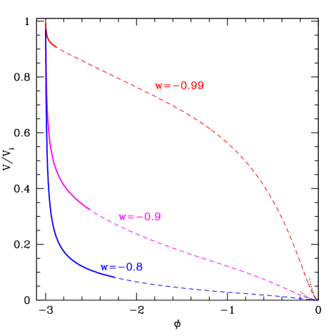
Figure 4: Solutions for the potential function are exhibited that deliver constant values of the equation of state $w$. Solid portions of the curves correspond to the region over which the field has rolled by the present. Short dotted arcs near $\phi=0$ show the $V\sim\phi^{2}$ asymptotic behavior. The potentials do not contain an explicit cosmological constant (i.e. $V(\phi)$ has a true zero minimum), but the equations of state can approach $w=-1$ due to the DBI dynamics.

IV Multi-Brane DBI

In the presence of multiple D3-branes or a non-BPS brane, the DBI action acquires an additional potential $U(\phi)$ multiplying the DBI term gumward ; saridakis ,

$$S = \int d^{4}x\,\sqrt{-g}\,\times$$ (13)

$$\left[-U(\phi)\,T(\phi)\sqrt{1-\dot{\phi}^{2}/T(\phi)}+T(\phi)-V(\phi)\right].$$

The energy-momentum tensor takes a perfect fluid form with energy density $\rho_{\phi}$ and pressure $p_{\phi}$ given by

$$\rho_{\phi}=(\gamma U-1)\,T+V\quad;\quad p_{\phi}=(1-\gamma^{-1}U)T-V\,.$$ (14)

The Lorentz factor $\gamma$ is still given by Eq. (2) and the equation of state for the DBI field is

$$w\equiv\frac{p_{\phi}}{\rho_{\phi}}=-\frac{\gamma^{-1}U-1+v}{\gamma U-1+v}\,.$$ (15)

The extra freedom from the additional potential $U$ means that interesting results occur in both the nonrelativistic and relativistic cases, not just $\gamma\to\infty$ as in the standard DBI model.

IV.1 Equations of Motion and Attractors

The equation of motion for the field follows from either functional variation of the action or directly from the continuity equation for the energy density,

$$\rho^{\prime}_{\phi}=-3(\rho_{\phi}+p_{\phi})=-3(\gamma-\gamma^{-1})\,UT\,,$$ (16)

where a prime denotes a derivative with respect to the e-folding parameter, $d/d\ln a$.

To begin, we define the contributions of the tension and potential to the vacuum energy density relative to the critical density,

$$x^{2}=\frac{\kappa^{2}}{3H^{2}}(\gamma U-1)\,T\quad;\quad y^{2}=\frac{\kappa^{2}}{3H^{2}}V\,,$$ (17)

where $\kappa^{2}=8\pi G$ and $H$ is the Hubble parameter. We allow the parameter $x^{2}<0$ so as to unify the treatment of when $\gamma U>1$ and $\gamma U<1$. The equations of motion are given by

$$\frac{1}{2}(x^{2})^{\prime} = -\frac{3}{2}x^{2}(1-x^{2})\frac{1-\gamma^{-1}U}{\gamma U-1}-\frac{3}{2}x^{2}y^{2}$$ (18)

$$+\frac{\sqrt{3}}{2}\lambda\,y^{2}\sqrt{\frac{(\gamma^{2}-1)\,x^{2}}{\gamma^{2}(\gamma U-1)}}$$

$$y^{\prime} = \frac{3}{2}\,x^{2}y\,\frac{\gamma^{2}-1}{\gamma}\frac{U}{\gamma U-1}+\frac{3}{2}\,y\,(1-x^{2}-y^{2})$$ (19)

$$-\frac{\sqrt{3}}{2}\lambda\,y\sqrt{\frac{(\gamma^{2}-1)\,x^{2}}{\gamma^{2}(\gamma U-1)}}$$

$$\kappa\phi^{\prime} = \sqrt{\frac{3(\gamma^{2}-1)\,x^{2}}{\gamma^{2}(\gamma U-1)}}\,,$$ (20)

where $\lambda=-(1/\kappa V)dV/d\phi$ and

$$\gamma U=1+\frac{V}{T}\frac{x^{2}}{y^{2}}\,.$$ (21)

When $U=1$ these equations reduce to those in akl . The case $\gamma U=1$ can be handled by the above equations since the denominator $\gamma U-1$ always occurs in the finite ratio $x^{2}/(\gamma U-1)$.

We are interested in the DBI field as late time accelerating dark energy, not for inflation, so we take the initial conditions in the matter dominated universe and define the present by $\Omega_{\phi}=0.72$. The attractor solutions to the equations of motion have the critical values

$$x^{2}_{c1} = \frac{\lambda^{2}}{3U^{2}}\frac{\gamma U-1}{\gamma^{2}-1}\quad;\quad x^{2}_{c2}=\frac{3\gamma^{2}}{\lambda^{2}}\frac{\gamma U-1}{\gamma^{2}-1}$$ (22)

$$y^{2}_{c1} = 1-\frac{\lambda^{2}}{3U^{2}}\frac{\gamma U-1}{\gamma^{2}-1}\quad;\quad y^{2}_{c2}=\frac{3}{\lambda^{2}}\frac{\gamma^{2}-\gamma U}{\gamma^{2}-1}$$ (23)

$$\Omega_{\phi,c1} = 1\quad;\quad\Omega_{\phi,c2}=\frac{3\gamma U}{\lambda^{2}}$$ (24)

$$w_{\phi,c1} = -1+\frac{\lambda^{2}}{3\gamma U}\quad;\quad w_{\phi,c2}=0\,.$$ (25)

These are stable, late time attractors, with the $w\neq 0$ solution reached for $\lambda^{2}<3\gamma U$. The form of these solutions reveals that paths to the attractor classes are more diverse compared to standard DBI theory. For example, new windows appear for obtaining $w=-1$ if $U(\phi_{c})\to\infty$ sufficiently quickly. In particular, this cosmological constant behavior can even be realized when $\gamma\to 1$, without the potential running to infinite field values. Now the important limit is when $\gamma U\to\infty$ rather than $\gamma$ alone. These attractors can therefore be achieved when $\gamma$ remains nonrelativistic but $U$ gets large for the asymptotic field value.

The attractor value for $w$ depends on two key parameters: $\lambda^{2}/U$ and $v\lambda^{2}/U^{2}$. The explicit solution is given by

$$w=-1+2\,\left[1+\sqrt{1+12\,\frac{v-1}{\lambda^{2}}+\left(\frac{6U}{\lambda^{2}}\right)^{2}}\right]^{-1}\,,$$ (26)

and the value of the Lorentz boost factor is

$$\gamma=\frac{\lambda^{2}}{6U}+\sqrt{\left(\frac{\lambda^{2}}{6U}\right)^{2}+\frac{\lambda^{2}\,(v-1)}{3U^{2}}+1}\,.$$ (27)

Table 1 shows the parameter combinations that lead to attractors with accelerated expansion. As stated, although the essential classes of attractors (the four groups divided by the horizontal rows) are the same as with standard DBI (cf. Table 1 of akl ), the paths to obtaining them are multiplied. These can deliver cosmological constant like behavior nonrelativistically, due to the influence of the multibrane potential $U$, as well as new approaches to $w=$ constant, arbitrarily close to $w=-1$. (However, as we discuss in the next subsection, one can also absorb $U$ into standard DBI.)

$V/T$	$\lambda^{2}/U$	$\lambda^{2}v/U^{2}$	$\gamma$	$\gamma U$	$w$
$\infty$	moot	$\infty$	$\infty$	$\infty$	$-1$
$\infty$	$0$	0	1	$\infty$	$-1$
$\infty$	$\infty$	$\infty$	$\infty$	$\infty$	const
$\infty$	$\infty$	const	$\infty$	const	const
$\infty$	const	const	const	const	const
$\infty^{\dagger}$	0	0	1	$\infty$	$-1$
const	const	const	const	const	const
const	$\infty$	$\infty$	$\infty$	const	const
const	0	0	1	$\infty$	$-1$
0	const	0	1	const	const
0	0	0	$1$	const∗	$-1$

Table 1: Summary of accelerating attractor properties. The columns give the values of the quantities for the attractor solution, all of which possess asymptotic $\Omega_{\phi}=1$. Each grouping of rows corresponds to one of the classes of standard DBI from Table 1 of akl , with the first row of each group being the standard DBI solution. We see that multibrane DBI increases the number of ways of obtaining accelerating attractor solutions by almost a factor 3 over standard DBI and a factor 11 over quintessence. The dagger indicates that while $V/T=\infty$, $(V/T)/\lambda^{2}=$ const. The asterisk in the last row denotes that the constant is 0 unless $U\to\infty$. The values of constant $w$ are given by Eq. (26).

Class 1 in the first group of rows of the table achieves cosmological constant behavior. This can be realized, for example, through taking $T\sim\phi^{m}$, $V\sim\phi^{c}$, $U\sim\phi^{p}$ with any $p<-2$. In other words, even forms of the tension $T$ and potential $V$ that in standard DBI do not give acceleration, let alone $w=-1$, can give an asymptotic cosmological constant state if $U$ increases sufficiently rapidly, e.g. having an inverse power law form with $p<-2$. The steepness of $U$ trumps the behavior of $V$, $T$ so also the standard case giving $w$ constant (e.g. $T\sim\phi^{4}$, $V\sim\phi^{2}$) would instead yield $w=-1$.

Class 2 in the second group of rows of the table delivers a constant $w$, which can be made arbitrarily close to $-1$ depending on parameter values. An example would be given by the additional multibrane potential with $p=-2$. Here, though, if $V$ and $T$ were such that they would cause an attractor to $w=-1$, then this still holds. Alternately, if $V$ and $T$ could not attain an accelerating attractor, $U\sim\phi^{-2}$ can achieve this with a constant $w$. Note that the presence of $U$ also alters the value of constant $w$ (cf. Eq. 26) from the standard DBI case where $V$, $T$ give a constant $w$.

However, if $U$ does not get large sufficiently quickly, e.g. $p>-2$, then $V$ and $T$ determine the attractor behavior in the same manner as in standard DBI. Figures 5 and 6 illustrates these various behaviors, for cases where standard DBI would predict a constant $w$ attractor and no accelerating attractor, respectively. (We do not show the $V\sim\phi^{1}$ case because as stated this has identical asymptotic behavior to the standard DBI theory.)

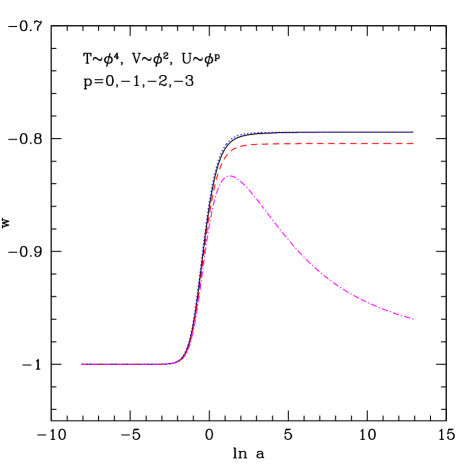
Figure 5: The presence of the multibrane potential $U$ alters the conditions for attractor solutions and opens up new routes to approach $w=-1$. When $\lambda^{2}/U\to 0$, then the cosmological constant is the asymptotic solution. When this combination goes to a constant value, then $w\to$ constant given by Eq. (26), and when the combination goes to $\infty$ then the standard DBI solution is unchanged. For a power law potential $U\sim\phi^{p}$, these correspond to $p<-2$, $=-2$, $>-2$.

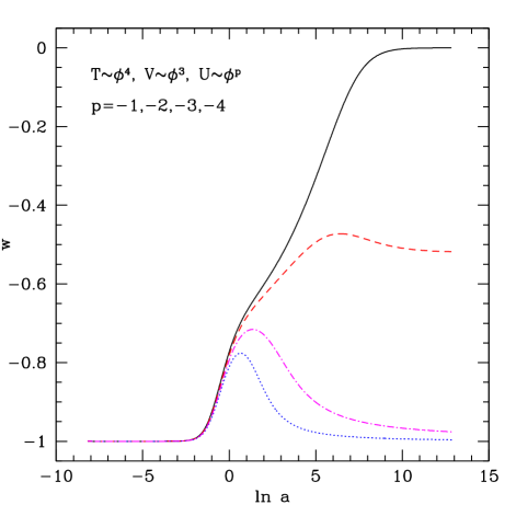
Figure 6: As Fig. 5 but for a form of the standard potential $V$ that would not give an accelerating attractor in standard DBI theory. Here, however, the multibrane potential can give constant $w$ (for $p=-2$) or a cosmological constant (for $p<-2$).

Class 3 is characteristic of exponential potential and tension, where the field runs off to infinity. However, the behavior of $U$ can determine the value of $w$, leading to either a constant $w\neq-1$ attractor or a cosmological constant state, unlike in standard DBI. Class 4 is similar to standard quintessence but again $U$ can deliver $w=-1$.

Just as in §III, one can design a function $U$ to fit a specific expansion history, or equation of state, through Eq. (15). Also note that a constraint on $U$ exists from the nonnegativity of the energy density in Eq. (14). This imposes the condition

$$\gamma U\geq 1-v\,.$$ (28)

This is automatically satisfied for $\gamma U\geq 1$ (we always take $V$, $T$ nonnegative). For $\gamma U<1$ though it limits the allowed forms of $U(\phi)$. When $\gamma U=1$ then $w=-1+\lambda^{2}/3$ at all times, not just asymptotically (when $\lambda^{2}>3$ there is no attractor). This looks like a standard quintessence attractor solution, but can actually be realized by a relativistic $\gamma$ model with $U<1$.

IV.2 Single Brane Equivalence

In examining the nonrelativistic limit of the action (13) we see that it approaches quintessence with a redefinition of the field and potential. This suggests a deeper mapping between the multibrane and standard single brane DBI actions. By defining

$$\varphi\equiv\int\sqrt{U}d\phi$$ (29)

we can rewrite the action (13) in terms of $\varphi$:

$$S=\int d^{4}x\,\sqrt{-g}\left[-TU\sqrt{1-\dot{\varphi}^{2}/(TU)}+T-V\right].$$ (30)

Comparing this action with Eq. (1), we see that it is equivalent to the original DBI action with tension $\hat{T}$ and potential $\hat{V}$ given by

$$\hat{T} =TU,$$ (31)

$$\hat{V} =TU-T+V\,.$$ (32)

Therefore, the general analysis of akl applies to the multibrane situation when viewed in terms of the equivalent single brane, hatted quantities. Specifically, the formulae (17)–(25) hold for

$$x^{2}=\frac{\kappa^{2}}{3H^{2}}(\gamma-1)\,\hat{T}\quad;\quad y^{2}=\frac{\kappa^{2}}{3H^{2}}\hat{V}\,,$$ (33)

with the replacement $U\rightarrow 1$, $v\to\hat{v}$, $\phi\to\varphi$, and $\lambda\to\hat{\lambda}$ where $\hat{\lambda}=-(1/\hat{V})d\hat{V}/d(\kappa\varphi)$. In this formulation, the attractor values for $w$ and $\gamma$, Eqs. (26) and (27), take the same form as in standard DBI.

As an explicit example of the mapping between the multibrane and single brane views, let us consider the case where the (unhatted) tension and the potentials are given by power laws,

$$T\sim\phi^{m},\quad V\sim\phi^{c},\quad U\sim\phi^{p},$$ (34)

and investigate how the attractor values of $\gamma$ and $w$ change as the exponents are varied. This gives an alternate view and derivation of the results in Sec. IV.1. We assume $m$ and $c$ are positive for simplicity. From Eq. (29), the redefined field $\varphi$ is related to the original field $\phi$ as $\varphi\sim\phi^{(p+2)/2}$ and the hatted quantities become

$$\hat{T} =TU\sim\varphi^{\frac{2(m+p)}{p+2}},$$

$$\hat{V} =TU-T+V\sim\varphi^{\frac{2(m+p)}{p+2}}-\varphi^{\frac{2m}{p+2}}+\varphi^{\frac{2c}{p+2}},$$

$$\hat{v} =\hat{V}/\hat{T}\sim 1-\varphi^{-\frac{2p}{p+2}}+\varphi^{\frac{2(c-m-p)}{p+2}}.$$ (35)

Note that, if $p<-2$, $\varphi$ is inversely proportional to $\phi$ and the small-field limit for one is the large-field limit for the other. Thus it is natural to separately study the cases $p>-2$ and $p<-2$.

For the case $p>-2$, all the powers of the terms in $\hat{V}$ are positive and $\varphi$ would go to zero asymptotically. Then the logarithmic derivative $\hat{\lambda}\sim 1/\varphi$ diverges, giving the ultrarelativistic class of attractor solution $\gamma\rightarrow\infty$. To obtain $w=-1$, $\hat{v}/\hat{\lambda}^{2}$ should diverge, which happens if $m-c>2$. Note that this result is independent of $p$. Therefore we conclude that if $U$ is less singular than $1/\phi^{2}$ there is no effect of $U$, in agreement with Sec. IV.1.

If $p=-2$, then $\phi\sim e^{\varphi}$ and the hatted potentials and tension appear exponential. These give constant $w$ attractors, even if (unhatted) $V$ and $T$ would not normally give acceleration. If $V$ and $T$ would give $w=-1$ by themselves, then this is maintained.

If $p<-2$, then as noted above the small-field and large-field limits are reversed. Thus we obtain $w=-1$ in any case: if $V$ and $T$ provide $w=-1$ themselves, then this is maintained, while if they do not give acceleration then $U$ operates in the opposite limit and drives the field to a $w=-1$ attractor. Again, see Figs. 5-6 and Sec. IV.1.

As a curiosity, note we could take the converse view and split the single brane picture into multiple branes. For example, the usual quartic single brane tension $\hat{T}\sim\varphi^{4}$ could be viewed as $T\sim\phi^{m}$ and $U\sim\phi^{m-4}$ as a way of relaxing the conditions on the brane tension. It is this extra freedom from $U$ that generates further paths to the same attractors as in standard DBI.

Another interesting case arises by choosing $T=V=\text{const}$ and $U(\phi)$ as a runaway type potential connecting $U(0)=1$ and $U(\infty)=0$. Then the action can be interpreted as the action for an unstable D-brane in string theory sen and the field $\phi$ represents its tachyonic mode. A standard form for $U(\phi)$ is buchel ; kims ; kutasov

$$U=1/\cosh{\alpha\phi}$$ (36)

where $\alpha$ is a constant. In this case, $\varphi\sim e^{-\alpha\phi/2}$ and $\hat{V}\sim\varphi^{2}$. Then we get $\gamma\to\infty$ and $w=0$.

V Sound Speed

Beyond the homogeneous field properties we can briefly consider perturbations to the dark energy density. These propagate with sound speed $c_{s}$ and define a Jeans wavelength above which the dark energy can cluster. The sound speed is defined in terms of the Lagrangian density $L$ (given by the term in square brackets in Eq. 1 or 13) and canonical kinetic energy $X=(1/2)\dot{\phi}^{2}$ as soundspeed

$$c_{s}^{2}=\frac{L_{,X}}{L_{,X}+2XL_{,XX}}\,,$$ (37)

The result is $c_{s}=1/\gamma$ for both the standard martinyam and generalized DBI actions, since $U(\phi)$ does not change the kinetic structure.

For the attractors depending on the relativistic limit, such as for $w\approx-1$ in the standard DBI case, this implies the sound speed goes to 0 and dark energy can clump on all scales. One of the interesting aspects of multibrane DBI is that this is no longer necessary; $w=-1$ can be achieved with $\gamma=1$ and so $c_{s}=1$. However, when $w\approx-1$ in whichever case then dark energy perturbations cannot grow regardless of the sound speed, so the sound speed is unlikely to give a clear signature of the DBI theory for the cases we consider. Indeed even models of dark energy with $c_{s}=0$ cannot be readily distinguished from those with $c_{s}=1$, when $w\approx-1$ and the dark energy does not couple to matter beandore ; huscranton ; coragm (see matarrese ; lazkoz for the case of coupling).

VI Conclusions

We have investigated possible constraints on DBI string theory from cosmological observations, considering the entire field evolution not just the asymptotic future behavior. In particular, Eq. (10) gives a bound on the deviation of the locally warped region generated by the form-field fluxes from the AdS geometry. It is very interesting if more accurate cosmological data can restrict fundamental string parameters.

To improve the fine tuning problem of initial conditions, we have enlarged attractor solutions to the case of generalized DBI theory which includes an additional potential arising from either multiple coincident branes, or non-BPS branes, or D5-branes wrapping a two-cycle within the compact space and carrying a non-zero magnetic flux along this cycle gumward . We have obtained exact cosmological constant behavior from some attractors of the extended DBI theory. Also, we have noticed that the extended DBI theory can have the identical attractor behavior to single-brane DBI with a different tension and potential.

An interesting novel feature of the DBI attractors is that the sound speed can be driven to zero which enhances dark energy clustering, although this is suppressed when $w\approx-1$. We also showed that a straightforward quadratic plus quartic potential acts like a thawing scalar field, and how more complicated potentials could be designed for a specific cosmic expansion history.

We have analyzed in greater detail than in akl how accurate cosmological observations on the dark energy can constrain some aspects of fundamental string theory within the DBI framework. Input from high energy physics on the forms of the functions is necessary as well. The connections between string theory and astrophysical data offer exciting prospects for revealing the nature of the cosmological constant and the accelerating universe.

- (1) I. Zlatev, L. Wang, & P.J. Steinhardt, Phys. Rev. Lett. 82, 896 (1999)
- (2) C. Ahn, C. Kim, E.V. Linder, arXiv:0904.3328
- (3) J. Martin & M. Yamaguchi, Phys. Rev. D 77, 123508 (2008)
- (4) E. Silverstein & D. Tong, Phys. Rev. D 70, 103505 (2004)
- (5) M. Alishahiha, E. Silverstein, & D. Tong, Phys. Rev. D 70, 123505 (2004)
- (6) R.R. Caldwell & E.V. Linder, Phys. Rev. Lett. 95, 141301 (2005)
- (7) R.N. Cahn, R. de Putter, & E.V. Linder, JCAP 0811, 015 (2008)
- (8) B. Gumjudpai & J. Ward, Phys. Rev. D 80, 023528 (2009)
- (9) E.N. Saridakis & J. Ward, Phys. Rev. D 80, 083003 (2009)
- (10) A. Sen, JHEP 0204, 048 (2002)
- (11) A. Buchel, P. Langfelder, J. Walcher, Ann. Phys. 302, 78 (2002)
- (12) C. Kim, H. Kim, Y. Kim, O.-K. Kwon, JHEP 0303, 008 (2003)
- (13) D. Kutasov, V. Niarchos, Nucl. Phys. B666, 56 (2003)
- (14) J. Garriga & V. Mukhanov, Phys. Lett. B 458, 219 (1999)
- (15) R. Bean & O. Doré, Phys. Rev. D 69, 083503 (2004)
- (16) W. Hu & R. Scranton, Phys. Rev. D 70, 123002 (2004)
- (17) P-S. Corasaniti, T. Giannantonio, A. Melchiorri, Phys. Rev D 71, 123521 (2005)
- (18) D. Bertacca, N. Bartolo, A. Diaferio, S. Matarrese, JCAP 10, 023 (2008)
- (19) L.P. Chimento, R. Lazkoz, I. Sendra, arXiv:0904.1114