Host Galaxies of z=4 Quasars

Abstract

We have undertaken a project to investigate the host galaxies and environments of a sample of quasars at $z\sim 4$. In this paper, we describe deep near-infrared imaging of 34 targets using the Magellan I and Gemini North telescopes. We discuss in detail special challenges of distortion and nonlinearity that must be addressed when performing PSF subtraction with data from these telescopes and their IR cameras, especially in very good seeing. We derive black hole masses from emission-line spectroscopy, and we calculate accretion rates from our $K_{s}$-band photometry, which directly samples the rest-frame $B$ for these objects. We introduce a new isophotal diameter technique for estimating host galaxy luminosities. We report the detection of four host galaxies on our deepest, sharpest images, and present upper limits for the others. We find that if host galaxies passively evolve such that they brighten by 2 magnitudes or more in the rest-frame $B$ band between the present and z=4, then high-z hosts are less massive at a given black hole mass than are their low-z counterparts. We argue that the most massive hosts plateau at $\lesssim 10\hbox{$\rm L^{*}$}$. We estimate the importance of selection effects on this survey and the subsequent limitations of our conclusions. These results are in broad agreement with recent semi-analytical models for the formation of luminous quasars and their host spheroids by mergers of gas-rich galaxies, with significant dissipation, and self-regulation of black hole growth and star-formation by the burst of merger-induced quasar activity.

1 Introduction

In the past decade, we have begun to understand the important role that black holes play in galaxy evolution. Observations suggest that supermassive nuclear black holes are likely present in nearly all normal galaxies, and that black hole mass is correlated with host galaxy bulge mass (Kormendy & Richstone, 1995; Magorrian et al. , 1998) and stellar velocity dispersion (Ferrarese & Merritt, 2000; Gebhardt et al. , 2000; Tremaine et al. , 2002; Marconi & Hunt, 2003; Häring & Rix, 2004). Low-redshift quasars too are consistent with these results: at low redshift, the most luminous quasars reside in massive, early-type host galaxies, and fit the black-hole-mass-spheroid relation for Eddington fractions of about $\sim 40\%$ (McLeod & Rieke, 1995; McLeod, Rieke, & Storrie-Lombardi, 1999; McLure et al. , 1999; McLeod & McLeod, 2001; McLure & Dunlop, 2001; Floyd et al. , 2004; Kiuchi et al., 2009; Silverman et al., 2009). These results have implications for the evolution of luminous, high-redshift quasars. If a galaxy already had a supermassive black hole early on, then according to the local black-hole/bulge relation, it must by today be one of today’s most massive galaxies.

In the context of the $\Lambda$CDM framework for hierarchical structure growth, specific predictions can be made for the evolution of quasar hosts and their environments through cosmic time (Mo & White, 2002; Kauffmann & Haehnelt, 2002). If dissipationless gravitational collapse of cold dark matter were the only process at work, then one would expect the ratio of black hole mass to stellar spheroid mass, $M_{BH}/M_{*}$, to be roughly constant as spheroids merge and their nuclei coalesce. However, luminous quasars like the ones in current samples of quasars at $z\geq 4$ are likely the product of major mergers of gas-rich disk galaxies of comparable mass (Hopkins et al., 2005; Croton, 2006; Di Matteo et al., 2008; Hopkins et al., 2008; Somerville et al., 2008). The central black holes merge, and merger-induced gas accretion results in a burst of quasar activity. Quasar radiative energy and winds eventually halt further mass accretion and clear out the cold gas, halting star-formation. The merger disrupts the original gaseous disks, and the result is a low angular-momentum spheroid of stars that subsequently evolves passively. Semi-analytical models for these processes, along with numerical simulations of the collapse of cold-dark-matter halos, are successful in reproducing many observations of galaxies, galaxy clusters and quasars. In these models, high-z quasars are expected to have less luminous hosts than their low-z counterparts (Kauffmann & Haehnelt, 2000), with the ratio of black hole mass to stellar spheroid mass, $M_{BH}/M_{*}$, decreasing with redshift (Croton, 2006; Somerville et al., 2008).

By necessity, models for quasar host evolution rely on semi-empirical prescriptions for key physical processes, because the resolution of numerical simulations cannot follow all of the crucial physics from the spatial scales of galaxy clusters down to galactic then to atomic scales. Direct observations of high redshift quasar hosts such as the study described here provide one interesting empirical check on the overall validity of the theoretical picture of hierarchical galaxy and black hole formation and evolution.

Detecting the host galaxy “fuzz” is technically challenging at high redshift however because it appears small and faint compared to scattered light from the nucleus in the wings of the point spread function (PSF). Ideally, we would study the fuzz in the rest-frame near-IR, which would both highlight the mass-tracing stellar populations of the hosts and provide the best possible galaxy-to-nuclear light contrast (McLeod & Rieke, 1995). For high-z objects, that would mean observing in the mid-IR, but there are not yet telescopes with the necessary combination of sensitivity and angular resolution to make such observations feasible. Most high-z host studies so far have therefore used near-IR imaging.

At $z\sim 2-3$, the first near-IR imaging of handfuls of objects using 4m-class telescopes produced detections only in the case of radio-loud (RL) quasars (Lehnert et al., 1992; Lowenthal et al. , 1995; Aretxaga, Terlevich, & Boyle, 1998; Carballo et al., 1998). Fuzz was subsequently seen around a few radio-quiet (RQ) quasars using adaptive optics (AO) on 4m telescopes (Aretxaga et al. , 1998; Hutchings et al. , 1999; Kuhlbrodt et al. , 2005), and AO on the Gemini North 8m yielded only one of 9 hosts at $z\sim 2$ (Croom et al., 2004). The well-characterized and stable PSF of NICMOS allowed successful detections of larger samples of RQ hosts in this redshift range (Kukula et al. , 2001; Ridgway et al. , 2001; Peng et al. , 2006), which led to the first tantalizing comparisons with hierarchical models. Peng et al. (2006) suggest that at $z=2$, $M_{BH}/M_{*}$ was several times larger than it is today, and that hosts were not yet fully formed, though those results have been the subject of some debate. For example Falomo et al. (2008) have recently used AO imaging on the VLT to detect the hosts of three luminous quasars at $2<z<3$, which they use to help argue for passively evolving $\sim 5\hbox{$\rm L^{*}$}$ elliptical hosts. Moreover, Malmquist bias in high-z samples would skew detections towards bright quasars in small hosts (Lauer et al. , 2007; Treu et al., 2007; Woo et al., 2008); we discuss this effect further in §7.6.

To provide more leverage for probing the hierarchical models, we would like to measure host properties at $z\sim 4$. So far, host detections have been claimed for just a few objects in this range, all with unknown radio type. Peng et al. (2006) used NICMOS to measure host magnitudes and sizes for two gravitationally lensed quasars at $z=4.1$ and 4.5. Hutchings has used Gemini to observe seven targets with $z\sim 5$ (Hutchings, 2003, 2005); unfortunately, the results are hard to interpret in light of the distortion and nonlinearity effects that we have found to be significant for the same instrument (see below).

With the improvement in sensitivity provided by 6-8m class telescopes, we have begun to expand the sample of quasars imaged at high z. Our long-term program includes new multi-wavelength imaging to search for hosts and to characterize environments; new and archival visible spectroscopy to be used for virial mass estimates of the central engines from emission line properties; and modeling of the accretion disks and hot coronae using data from IR to X-ray, including new X-ray data from ongoing Chandra and XMM observing programs.

In this paper, we describe a sample of 34 $z\sim 4$ quasars that we have imaged in the near-IR. We present the observations and report on the search for hosts. The environments will be described in a subsequent paper (Bechtold & McLeod 2010, in preparation). We adopt the cosmology $\Omega_{\Lambda}=0.7,\Omega_{\rm m}=0.3$, $H_{0}=70\rm~{}km~{}s^{-1}~{}Mpc^{-1}$ throughout. All magnitudes are reported in the Vega system, unless otherwise noted.

2 The Sample

We have observed a sample of quasars selected to have redshifts in the range $3.6\lesssim z\lesssim 4.2$. The sample is listed in Table 1 with names as given in the NASA/IPAC Extragalactic Database (NED). The redshift range was chosen so that the 4000Å break falls between observed $H$- and $K$-bands, so that broad-band colors give maximum leverage for estimating photometric redshifts and stellar populations. Out of the $\sim 300$ quasars known in this interval when we began the project, we observed a randomly-chosen sub-sample of 34 objects, yielding a median $<z>=3.9$ and spanning a range of magnitude as shown in Fig. 1. We plot our sample against the $\sim 1600$ quasars at these redshifts listed in the most recent Sloan Digital Sky Survey (SDSS) Quasar Catalog (Schneider et al. , 2007).

We are observing first in the $K$-band, which samples the rest frame $B$ for these objects. The median observed total nuclear $K_{s}=17.2$ for the quasars in our sample corresponds to $M_{B}=-26.9$ (Vega magnitudes), similar to the local luminous quasar 3C273.

2.1 Radio Loudness

To characterize the radio properties of our sample, we adopt the definition of radio loudness given in Ivezic et al. (2002), who analyzed the radio properties of SDSS qusars. They define the apparent AB magnitude (Oke & Gunn, 1983) at 1.4 GHz as

$$t\equiv-2.5log_{10}\left({{F_{int}\over{3631Jy}}}\right)$$

where $F_{int}$ is the integrated 20cm radio flux measured from a two-dimensional Gaussian fit to the radio source. The radio-to-optical flux density is then defined as

$$R_{i}\equiv 0.4(i^{AB}-t)$$

where $i^{AB}$ is the AB magnitude at Sloan $i$ in the continuum. With these definitions Ivezic et al. (2002) find that radio-loud quasars have $R_{i}\cong 1-4$ and radio-quiet quasars have $R_{i}<1$.

The radio properties for the quasars in our sample are given in Table 2. We compiled the optical magnitudes from a number of sources. When available, we adopted the values for $i^{AB}$ published by members of the Sloan consortium; references are listed in Table 2. For most other objects, we used the $i^{AB}$-band photometry given on the SDSS web site (DR6). For two objects we measured photometry from archival HST images. For these and a few other cases, the only available photometry was from the literature in other filters, which we transformed to $i^{AB}$ using the zero-points given in the NICMOS web site unit converter, and assuming a quasar spectral energy distribution in the form of a power law

$F_{\nu}\propto\nu^{\alpha}$ where the spectral index $\alpha=-0.44$ for $1216\AA\leq\lambda_{rest}<5000\AA$

which is the average derived from the SDSS quasars by VandenBerk et al. (2001) (see also Pentericci et al. (2003)).

We corrected the optical magnitudes for Galactic reddening, using the $E(B-V)$ given by Schlegel et al. (1998) as tabulated in NED. The transformations $A_{r}=E(B-V)/2.751$ and $A_{i}=E(B-V)/2.086$ were adopted (Schneider et al. , 2003).

For most of the sample quasars, the most sensitive radio data comes from the Faint Images of the Radio Sky at Twenty-cm Survey (Becker et al., 1995, FIRST), which we accessed through NED. If the quasar did not fall in one of the FIRST fields, we used the data from NRAO VLA Sky Survey (NVSS; (Condon et al., 1998)). In a few cases the most sensitive radio data had been reported in targeted searches in the literature. For objects detected in FIRST, we adopted the FIRST catalog integrated flux. For others, we derived a 2$\sigma$ upper limit from the root-mean-square fluxes in the maps downloaded from NED.

Of the 34 sample quasars, 16 are radio-quiet, 5 are radio-loud, 4 have no radio data, and 9 have radio data which are not deep enough to know whether or not the quasar is radio-loud or radio-quiet.

Going into our survey, we wanted to test whether radio-loud quasars have different host galaxy properties than the radio-quiet majority. We therefore tended to give priority to observing quasars which we knew to be radio-loud, since they are rare and we knew that it would be difficult to get a statistically large sample of them. In the end, at least 5 quasars in the sample of 34 are radio-loud, compared to approximately 1 expected to be radio-loud, had we observed a sample representative of the radio properties of the bright quasar population at $z\sim 4$ as a whole (Jiang et al., 2007).

2.2 Black Hole Mass Estimate

We estimated the black hole mass $\rm M_{BH}$ for the quasars in our study from emission-line spectroscopy. As described below, we measured the full-width-half-maximum (FWHM) value of the broad CIV emission line and the quasar UV continuum luminosity from new and existing spectra. We then used these to compute black hole mass according to the relation

$$log_{10}\left({\rm M_{BH}\over M_{\sun}}\right)=log_{10}\left[\left({{\rm FWHM_{CIV}}\over{1000km~{}s^{-1}}}\right)^{2}\left({\lambda L_{\lambda 1350}\over{10^{44}erg~{}s^{-1}}}\right)^{0.53}\right]+6.66$$

from Vestergaard & Peterson (2006), who find that the UV continuum luminosity $L_{\lambda 1450}$ can be freely substituted for $L_{\lambda 1350}$. From this we derived

$$log_{10}\left({\rm M_{BH}\over M_{\sun}}\right)=2log_{10}\left({{\rm FWHM_{CIV}}\over{1000km~{}s^{-1}}}\right)+0.53\left[11.37+{2*\rm{DM}\over{5}}-{{\rm{AB}_{1450}+48.60}\over{2.5}}-log_{10}(1+z)\right]+6.66$$

Here, ${\rm AB_{1450}}\equiv-2.5log_{10}f_{\nu}-48.6$, where $f_{\nu}$ is the (reddening-corrected) continuum flux in $erg~{}s^{-1}cm^{-2}Hz^{-1}$ measured at an observed wavelength of $\lambda=1450\AA(1+z)$ as in Fan et al. (2001). $DM$ is the (luminosity) distance modulus.

The $\rm AB_{1450}$ magnitudes were compiled from the literature or measured by us as shown in Table 3. Where available, we adopt the reddening-corrected $\rm AB_{1450}$ tabulated by members of the Sloan consortium, who give values based on spectrophotometry of the quasars at a rest frame wavelength of 1450Å. For 10 of the objects, we measured the continuum fluxes ourselves from spectra obtained from the SDSS Skyserver. For the objects for which no flux-calibrated spectra were available, we used the $i^{AB}$ magnitudes from Table 2 and transformed to $\rm AB_{1450}$ assuming $\alpha=-0.44$ as described in §2.1. For objects with large CIV equivalent widths that contaminate the broadband measurements, the $\rm AB_{1450}$ derived from photometry will be systematically bright. A comparison of the spectroscopically-derived $\rm AB_{1450}$ to the photometrically-derived one for the SDSS objects shows the former to be fainter on average by $0.4\pm 0.3$ mag.

For most objects, we measured the FWHM of the C IV emission lines given in Table 3 using spectra from the SDSS Skyserver or electronic versions of published spectra from several authors who kindly made them available. In a few cases, we digitized published spectra using $``$Plot Digitizer” software. We also carried out new long-slit optical spectroscopy for five targets in the sample, including one for which no other spectroscopy is published, [VH95]2125-4529. For the new observations, we used the DEIMOS spectrograph on the Keck-II telescope (Davis et al., 2003) on the nights of 2008 Oct 24 and 2004 Oct 12 and 13. The objects were observed through a 0.7 arcsec wide slit with the 1200 l/mm first order grating, resulting in a dispersion of 0.33 $\AA$/pixel. A GG495 filter was used to block second order light. Exposures were 600-900 seconds, mostly through clouds or at twilight. We reduced the data using the DEEP2 project IDL reduction pipeline, which flatfielded, sky-subtracted, wavelength-calibrated and extracted the spectra as described in the DEEP2 webpage, http://astro.berkeley.edu/$\sim$cooper/deep/spec2d/. Spectra are shown in Figure 2.

To derive the CIV line width, we subtracted a local continuum fit, derived by fitting a linear curve through the spectra in rest wavelengths 1425Å  to 1500Å  and 1760 Å  to 1860 Å. We replaced absorption features with an interpolated continuum estimate, and then fit a gaussian to the C IV emission line.

The quality of the C IV line profiles for the quasars in our sample ranged from very high-signal-to-noise examples with easy-to-define continua, to barely detected lines in discovery-quality spectra. Moreover, the redshifts of our targets shift the C IV line to wavelengths with strong telluric absorption and night-sky emission features that are difficult to calibrate out completely. Some lines probably are suppressed by undetected absorption features intrinsic to the quasar. As many authors have noted, quasar emission lines are non-Gaussian, in the sense that they have “pointy” peaks. Some C IV lines in our sample were also significantly asymmetric.

For these reasons, we measured the FWHM values by hand, using IRAF’s splot. In cases where part of the line profile was very noisy, we measured the half-width of the better side of the profile and doubled it. In a few of the spectra with very good signal-to-noise, there is clearly a narrow (2000-3000 km s^-1 FWHM) component, and broader wings (10,000-15,000 km s^-1 FWHM). For several objects, we estimated two values of the line width, one for each component; both are listed in Table 3. For [VCV96]Q2133-4625, the C IV profile is so noisy, possibly because of an absorption trough, that it was impossible to derive a FWHM from the published spectrum.

Our resulting black hole mass estimates are given in Table 3. The systematic uncertainties in these estimates for black hole mass are well-known (Wandel et al., 1999; Collin et al., 2002; Dietrich & Hamann, 2004; Kaspi et al., 2005; Vestergaard & Peterson, 2006; Netzer et al., 2007; Kelly & Bechtold, 2007; McGill et al., 2008). The primary assumption is that the CIV emitting gas is in virial equilibrium with the central black hole mass, and is located at a radius that scales with luminosity. For the luminous quasars in our sample, this means extrapolating from the relations tested in emission-line regions studied with reverberation mapping locally (Peterson et al., 2004). Further, the bolometric luminosity of each quasar is assumed to be a constant multiple of the $\lambda$1450 continuum luminosity, which certainly is not the case (e.g. Kelly et al. (2008)).

In Figure 3 we plot the black hole masses of the quasars in our sample along with those for the $\approx 1600$ SDSS quasars in this redshift range recently tabulated by Shen et al. (2008). For the 6 objects in common, our black hole mass estimates generally agree within $\approx 0.2dex$.

2.3 Accretion Rates

We combined the black hole masses with the K-band observations described below to calculate the quasar mass accretion rates. Because the observed K-band samples the rest-frame B-band, the K-band magnitude allows us to compute a B-band luminosity independently of spectral shape. This avoids the errors that result when one must extrapolate from optical photometry to the rest-frame B assuming a spectral index $\alpha$. We apply a B-band bolometric correction factor of 10.7 (Elvis et al., 1994) and we compare the resulting bolometric luminosity to the Eddington luminosity computed from the black hole mass via $L_{Edd}=3.3\times 10^{4}({\rm M_{BH}}/M_{\sun})~{}L_{\sun}$. We have assumed that all of the rest-frame B-band light can be attributed to the nucleus, which is a reasonable estimation for such luminous objects. The resulting accretion rates as fractions of Eddington, $L_{bol}/L_{Edd}$, are tabulated in Table 3.

The median $L_{bol}/L_{Edd}$ for the sample is $0.47\pm 1.6~{}(1\sigma)$, and the minimum value is 0.1. These rates are good matches to those inferred from studies of host galaxies locally; McLeod & McLeod (2001) found that the most luminous local quasars radiate at $\gtrsim 0.1L_{Edd}$, and Floyd et al. (2004) deduce a median rate $0.47$ for the most luminous local quasars.

The calculation of accretion rates yields a handful of quasars with super-Eddington rates. Of these, BR2212-1626 is gravitationally lensed (Warren et al., 2001) and so the continuum luminosity, which we have not corrected for gravitational magnification, is overestimated. Since both $M_{BH}$ and $L/L_{Edd}\propto L^{0.5}$, both quantities are also overestimated. For BRJ0529-3553, we have only a discovery quality spectrum, and the C IV line width is very uncertain. For 5 others which have $L/L_{Edd}>>1$, the C IV profile has good enough signal-to-noise to detect a distinct narrow and broad component. If the FWHM of the broad component is used, very large black hole masses, and sub-Eddington accretion rates are implied. Detailed modeling of the quasar spectra energy distribution and higher quality spectra of all targets would improve the estimates of black hole mass and accretion rate. We do not list the statistical errors for $M_{BH}$ and accretion rate in Table 3 because these numbers are dominated by systematic uncertainties and the simplifying assumptions described above.

Excluding the $L/L_{Edd}>1$ objects, the median rate becomes $0.41\pm 0.3$, consistent with the distribution plotted by Shen et al. (2008) for $z>3$ SDSS quasars.

As a second way to estimate black hole masses for our sample quasars, we assume that all of the quasars are radiating at $0.4L_{Edd}$, with bolometric luminosities determined from $M_{B}$ as above. The derived values are then the minimum plausible black hole mass that the nuclei could have to be emitting at the luminosity observed. These values are listed in Table 3.

3 Near-IR Imaging Observations

We have obtained deep, near-IR images of 34 quasars over the period 2002 September - 2005 January at the Magellan I 6.5m and Gemini North 8m telescopes. We have observed each field in $K_{s}$, with 5 also observed in $H$ or $H_{c}$. Most of the objects (26) were observed with Magellan’s PANIC (Martini et al. , 2004), a $1024\times 1024$ HgCdTe array with a pixel scale of 0$\farcs$125 and a field-of-view (FOV) of 128″. Before PANIC was installed, we imaged a few objects (6) with the old ClassicCam (Persson et al. , 1992), a $256\times 256$ HgCdTe array camera yielding a FOV of only $\sim 30\arcsec$ per exposure. The rest of our targets (7) were observed on Gemini with NIRI (Hodapp, K. W. et al. , 2003), a $1024\times 1024$ InSb array operated at f/6, yielding a pixel scale of 0$\farcs$116 and a FOV of 119″ per exposure. The observations are summarized in Table 1.

With all three instruments, we observed using a 9- or 25- point dither pattern of short exposures ($10-30$ sec each, repeated $1-3$ times per dither position). The times were chosen to keep the quasar images in the nominal linear range, with repeats limited to ensure fair sampling of sky variation. The dithers were typically repeated for half a night, yielding up to a thousand frames per field and average total on-source times of 3 hours for PANIC and NIRI. With NIRI and PANIC, the FOV was big enough for us to use stars on the quasar frames to measure the PSF. Due to ClassicCam’s smaller FOV, we had to alternate quasar dithers with dithers on a nearby star to sample the PSF. The average on-source time for ClassicCam was thus shorter, only about 2 hours, resulting in shallower images. As we describe in the sections below, the ClassicCam images turned out to be of very limited use for the host searches. However, we include them in this paper both because they remain somewhat useful for investigations of the near environments of the quasars, and to illustrate the difficulties of using out-of-field stars for PSF subtraction.

We were fortunate to have excellent seeing for many of the observations, with the final, combined $K_{s}$ quasar images from PANIC and NIRI having full-width half-max (FWHM) ranging from $0\farcs 32-0\farcs 66$ with median value $<FWHM>=0\farcs 43$. ClassicCam images were worse. Photometric calibration was done for the PANIC and NIRI images using the 2MASS stars (usually $1-3$) found on each combined quasar frame. We also cross-checked these values against observations of Persson faint IR standards (Persson et al. , 1998), and estimate that the photometric calibration is accurate to $\sim 0.1\rm mag$. For the ClassicCam images, whose FOV are too small to contain 2MASS stars, we used only the Persson et al.  standards.

4 Data Reduction

For all three instruments, we reduced the data using standard techniques in IRAF with its add-on packages gemini/niri and panic, the latter kindly provided by Paul Martini. The data from each instrument were handled somewhat differently, with flats made from twilight exposures, flat lamp exposures, and object frames for PANIC, NIRI, and ClassicCam respectively. Sky frames were generally made by median-filtering $9-10$ dither positions after masking out sources. For the NIRI images, persistence proved to be a significant problem, which we solved to our satisfaction by including in each frame’s bad pixel mask the object masks from the 2 previous frames.

The PANIC and NIRI detectors are known to be nonlinear by $\approx 1\%$ at 15,000ADU and 11,000ADU respectively, and we kept our quasar+sky counts well below these limits. Still, for the tight tolerances in this project we needed to take some care with the linearity correction. For PANIC we used flat lamp exposures of varying lengths to determine our own second-order correction which differed from the nominal pipeline correction by 0.5% at 15,000ADU. The NIRI pipeline does not offer any nonlinearity correction and we lacked the data to determine our own. We discuss the residual effects of nonlinearity in §5.

In the course of our analysis we detected a geometric distortion in the PANIC images. The distortion was visible as a radial stretch in contour plots of stars taken around an image. Paul Martini gave us a second-order geometric distortion correction derived from the PANIC optical prescription, which we then implemented in the pipeline. We note that the NIRI pipeline does not offer a distortion correction, though distortion proved to be an issue there as well. We discuss the implications further in §5.

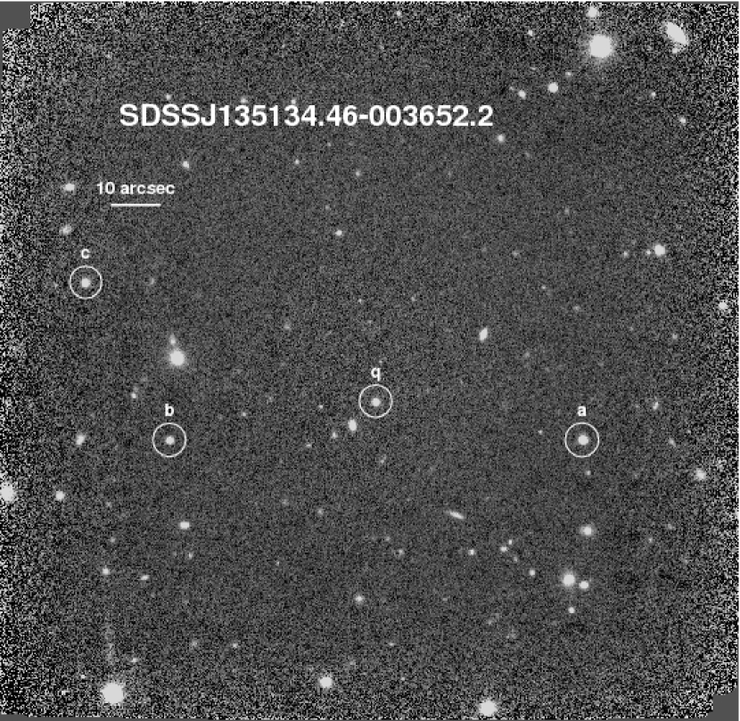
Figure 4: Sample PANIC image showing a $z=4.0$ quasar “q” and PSF stars “a” and “c.” The surface brightness limit in the center is $K=22\hbox{$\rm mag~{}arcsec^{-2}$}$, which is slightly better than average, but at $0\farcs 5$ the seeing is slightly worse than average. At this redshift, the field shown is $\sim 1\rm Mpc$ across.

The hundreds of reduced frames for each quasar were magnified by a factor of two, aligned on the quasar centroid, and combined after rejecting a handful of frames deemed bad because of bias level jumps in one quadrant or poor flattening. The deepest NIRI $K_{s}$ images reach a surface brightness limit of $K_{s}=22.9\hbox{$\rm mag~{}arcsec^{-2}$}$ (measured as a $1\sigma$ pixel-to-pixel variation). The median value is 21.7 $\rm mag~{}arcsec^{-2}$, typical for the PANIC images, while the ClassicCam images are more shallow. A typical PANIC image is shown in Fig. 4, where the FOV corresponds to $\sim 1.3\rm\ Mpc$ at $z=4$, well-suited for studies of quasar environments (see Bechtold & McLeod 2009).

5 PSF Characterization

Any search for host galaxies is only as good as the characterization and removal of the nuclear point source. We followed the traditional practice of selecting “PSF stars” from each image, and using them in model fits to the quasar images. However, in the course of our analysis we discovered some subtle effects of residual distortion and nonlinearity. Because we have not seen these issues addressed in other high-z host searches, including ones also done with NIRI, we discuss them in some detail here. For a recent look at the PSF perils that host galaxy studies might encounter even with HST, see Kim et al. (2008).

5.1 Geometric distortion, or What to Do When The Seeing is Too Good

Beginning with PANIC, our experiments with multiple PSF stars showed that poorer fits tend to result when the PSF star is farther from the quasar. Even though we had performed a distortion correction on the PANIC images, we found that a small residual geometric distortion compromised the fits. The distortion we detected would be insignificant (and indeed not noticeable) for most projects, with camera optics generally designed to create instrumental PSFs small compared to the seeing size. In our case, however, the excellent seeing and tight tolerances required for high-z host detection made the distortion apparent.

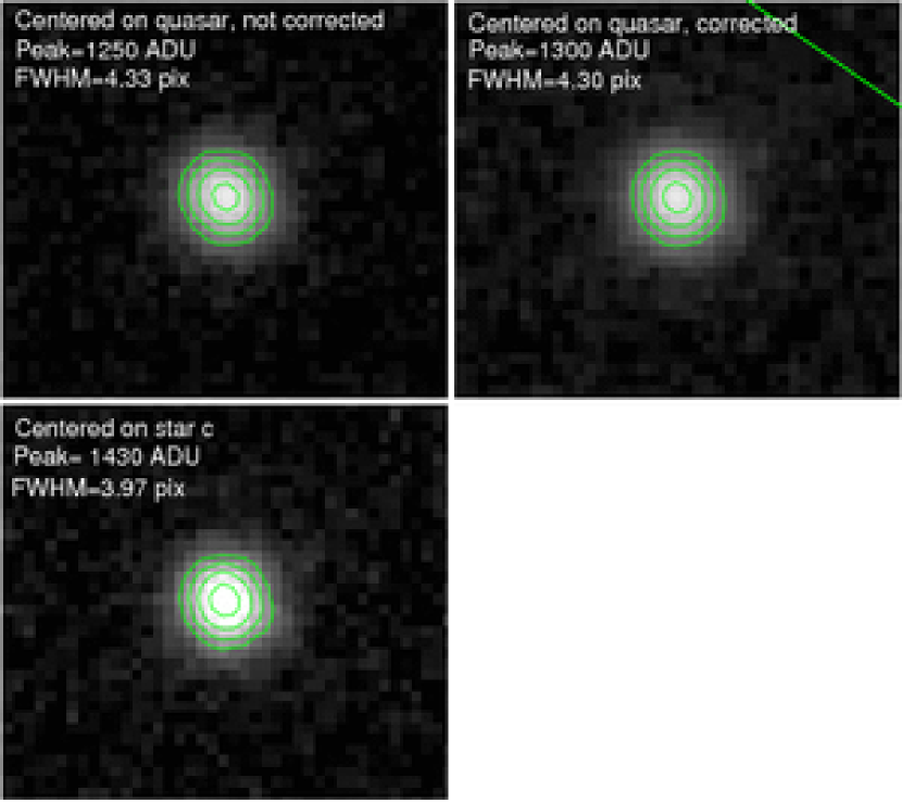
Figure 5: Effects of distortion corrections and recentering for star “c” from Fig. 4. Top left: frames have been aligned to the quasar centroid before combining, and no distortion correction has been performed. The star “c” image is stretched. Top right: the nominal distortion correction has been applied before aligning to the quasar centroid and combining, which has tightened up the star “c” image; however, it is still broader than the image of the quasar taken from the same frame. Bottom left: the distortion-corrected frames have instead been aligned to the centroid of star “c” before combining, effecting a second-order distortion correction for that star. The star “c” image now has the same FWHM and shape as the quasar did in the image aligned on the quasar centroids.

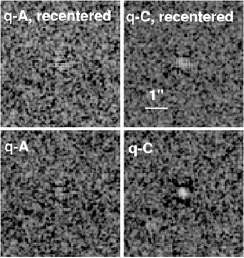
Figure 6: Improvement of fits for the quasar shown in Fig. 4 and 5 after creation of “recentered” PSF frames for stars “a” and “c.” The better fit with star “a” is likely due to its relative proximity to the center of the frame.

To improve the fits, we were able to effect a higher-order distortion correction by recentering each quasar’s hundreds of frames on PSF stars to create “PSF frames” for each target, as suggested to us by Brian McLeod. With distorted images, the pixel scale at the edges is different than that near the center. Therefore, when shifting and combining frames from different dither positions, the shifts computed based on the objects near the center (in this case quasars) will be the wrong number of pixels to align the objects near the edges, yielding a combined image with stretched edges. The recentering technique to help correct for this works as follows. First, as described above, we align the hundreds of images to the quasar centroids, and combine them to create a “quasar frame.” From this we extract a postage-stamp image of the quasar to use for fitting. We then start again with the same hundreds of images and align them this time to the centroid of a particular PSF star, and use these new shifts to combine them to make the “PSF frame” for that star. We then extracted a postage-stamp image of the PSF star from the latter frame for use with the fitting. An example is shown in Fig. 5. We used this technique with good success on most of the PANIC images. Examples of fits performed with and without our re-centering technique are shown in Fig. 6.

The NIRI images also suffer from distortion that proved significant for this project. No distortion correction is used in the NIRI pipeline. We applied our re-centering technique and found that it did improve the NIRI fits considerably, but PSF-PSF tests (where we subtracted PSF stars from each other) showed that residual distortion remains in the K image of SDSSJ012019.99+000735.5 and the H image of BRI0241-0146. For these two images, the only PSF star is far from the quasar.

The ClassicCam images provided their own set of challenges because the PSF stars were observed alternately with the quasars, and inevitable seeing variations resulted. We were able to obtain more reasonable results in most cases by rejecting frames according to the seeing, so that the resulting quasar and PSF star frames had the same FWHM. However, the ClassicCam results are never as satisfactory or robust as the Panic and NIRI results, and will be more useful for studies of the quasar’s near environment than for host detection.

5.2 Nonlinearity

Unfortunately, we also discovered that the near-IR images exhibit a small nonlinearity even after the nominal correction has been applied. This effect was more subtle than the distortion and became apparent only under scrutiny of the ensemble of data for our many objects. Such an effect could easily have escaped our detection in a study with fewer objects. We noticed that our best fits were found for PSF stars with similar brightness to the quasar. PSF stars brighter or fainter than the quasar could leave compact central emission or, more insidiously, rings that mimicked host galaxies in the difference images. Star-minus-star experiments performed on multiple PSFs from the same image confirmed our suspicion.

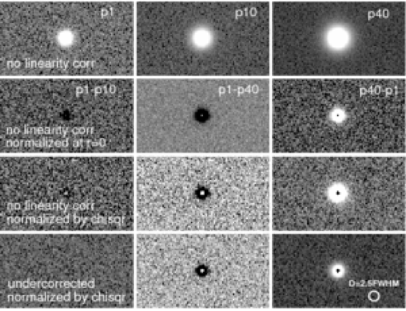
Figure 8: Effects of imperfect linearity corrections on PSF fits. Top row: simulated stars with the same FWHM and noise characteristics as our observed quasars and having relative flux 1, 10, and 40 times. Nonlinearity has intentionally been applied according to the middle curve from Fig. 7. Bottom three rows: results of correcting and subtracting these stars from each other via different schemes. In rows 2 (PSFs normalized to the central pixel before subtraction) and 3 (normalization based on a fit that minimizes residuals) we have performed no linearity correction. Residuals are obvious and the details depend on the normalization. In row 4, we have applied a linearity correction that differs from the one used to generate the stars by $\lesssim 0.5\%$. The spurious residuals are only obvious with the brighter PSFs, and do not extend beyond a diameter of 2.5*FWHM.

This is difficult to illustrate with observed stars because of the residual distortion discussed above. However, we investigated this further by simulating observations of stars of different magnitudes and fitting and subtracting them after applying different plausible linearity corrections. For example, we have used the nonlinearity curve for PANIC shown in Fig. 7 to generate the suite of stars shown in Fig. 8 with radial intensity profiles given in Fig. 9. The counts for the fainter stars were chosen to keep the detector within the range where the response is approximately linear, as is done for the observed targets. For the brightest stars, we allowed the brightness to enter the nonlinear (but not close to saturated) regime. For the PANIC response, this corresponds to $\sim$15000 counts. At this level, the difference between the plausible prescriptions for the linearity correction amounts to $\lesssim 0.5\%$.

When we generated stars using one prescription and then “corrected” them for nonlinearity using another, the 2D residuals in star-star tests were clearly positive. In other words, the uncertainty in the linearity correction can lead to spurious detections when scaling and subtracting point sources that differ in flux. However, in the cases we tried, the spurious residuals were distinguished either by unphysically compact sizes (FWHM less than the image FWHM) as shown in Fig. 9, or else by donuts that could be mistaken for over-subtracted hosts. The latter did not extend past a diameter of $D=2.5~{}\rm FWHM$, as illustrated in Fig. 8.

5.3 Implications

Our results call into question the traditional approach of selecting “PSF stars…chosen to be as bright as possible without encountering detector saturation effects” (Hutchings, 2005). We have used this approach ourselves for low-z quasars (e.g. McLeod & Rieke (1995)) so that noise in the PSF wings is scaled down during the fitting process. However, our current analysis suggests that for PANIC and NIRI at least, a more robust practice is to chose PSF stars whose brightness is similar to the quasar, and whose positions are as close as possible. Which criterion takes priority might depend on the instrument and the observing conditions.

Distortion corrections and linearity corrections are essential, but not sufficient. The PSF star re-centering technique described above provides a higher-order distortion correction, but a possible added complication is that the accuracy of the registration can be dependent on the brightness of the stars. In addition, the characteristics of spurious residuals are dependent on the weighting process used during normalization of the PSF (e.g. normalize to the flux in the central few pixels, use the whole source for the fit, weight the fit by flux, etc.).

In principle, adaptive optics (AO) observations in which images of a PSF are interleaved with those of the quasar should be free from geometrical distortion when both are observed on the same part of the array. However, our results suggest that the case is not so clear. First, the AO observations will suffer from the same nonlinearity issues described above. Second, the adaptive correction procedure can be dependent on the object’s flux and the details of the profile, which can lead to an effective distortion. This underscores the desirability of observing PSF stars simultaneously with, and not just close in time to, the quasar; see however Ammons et al. (2009).

We conclude that the residual effects of distortion and nonlinearity should be addressed by individual near-IR host-hunters for their particular data sets. For the present study, we evaluate the residuals based partly on our knowledge of the brightness and proximity of the PSF stars. In most cases, we adopt as a criterion that positive residuals are considered significant only if they extend beyond a diameter of $D>2.5~{}\rm FWHM$, i.e. a radius $r>1.25~{}\rm FWHM$, which for the typical frame here means $r\gtrsim 0.55\arcsec$. We explore this further with the simulations discussed below. Of course, this particular criterion might not be appropriate for data taken under different seeing conditions or with different flux levels.

5.4 PSF Fits

To begin our search for host galaxies, we modeled each quasar as a point source with shape represented by the PSF star images. We determined a two-dimensional (2D) best-fit model for each quasar using the C program imfitfits provided by Brian McLeod and described in Lehár et al. (2000). This is the same program that we used on NICMOS images of low-redshift quasars (McLeod & McLeod, 2001). We used the 2x magnified images to ensure good sampling of the PSF, and extracted an $8\arcsec\times 8\arcsec$ sub-image for the fitting. Imfitfits makes a model by convolving a theoretical point source with the observed PSF, and then varying any combination of the parameters defining the background level and the position and magnitude of the point source to minimize the sum of the squares of the residuals over all the pixels. By subtracting the best-fit model from the quasar image, we can examine the result for any residual flux due to an extended component.

We achieved excellent results with at least one PSF star in most cases, as shown in Fig. 10. In a few cases where other sources within the 8″ box would bias the fits of the quasar, we have simultaneously fit those other sources as either point sources or galaxies. In these cases, we subtracted only the fitted quasar component for the figures; the other sources remain for comparison.

Our fitting process necessarily subtracts out any unresolved contribution from the host. A logical next step would be to perform a simultaneous fit of a point source plus a model galaxy as is commonly done with lower-redshift quasars. Unfortunately, we have found that for these data, multicomponent fits give uninterpretable results. The problem is that for our data, the likely range of scale lengths for the galaxies are small compared to the seeing disk and too little of the galaxy extends beyond the PSF. The result is that running a multicomponent fit, whether unconstrained or partially constrained (for example by holding fixed the centers, or the centers and the galaxy shape, or the centers and the nuclear flux, …), results in the ”galaxy” component being turned into a meaningless compact or even negative source to improve the fit in the quasar’s core, where PSF variations are the biggest. One idea to get around this problem is to downweight or mask out the core in the fits. However, our tests on real and simulated hosts have shown that the resulting ”galaxy” is sensitively dependent on the weighting scheme. (We had even seen hints of this with the much better resolved hosts in our low-z HST study (McLeod & McLeod, 2001).) Thus, we have developed a different way to estimate host magnitudes and morphologies via the simulations and isophotal diameter analyses described below.

As another tool for assessing host detection, we have generated one-dimensional (1D) radial brightness profiles, measured in circular annuli, of the quasar and PSF images. We present the surface brightness profiles in Fig. 11. For comparison we also generated a “fully-subtracted” profile by normalizing the PSF to the quasar within the central few pixels and subtracting. In most cases, the PSFs are excellent matches to the quasars down to the level of the sky noise.

We caution that the 1D profiles need to be interpreted carefully. For example, for our ClassicCam image of q0311-5537, the profile alone (see Fig. 11) looks like those of some host detections postulated in the literature. However, the 2D fit (see Fig. 10) shows that the residual flux is due to PSF mismatch. For the cases where we do have candidate host galaxies, we can use the 1D profiles to obtain estimates of the host flux. To do this, we subtract a fractional PSF profile that leaves a just-monontonic residual (as any plausible host would not decrease in brightness towards its center), and add up the residual light by integrating. This technique is necessarily crude, but the data do not warrant more sophisticated fits.

6 Detection Limits

In §5 above, we concluded from our PSF-PSF tests that any residual flux from our quasar fits outside a diameter of $D>2.5~{}\rm FWHM$ is likely significant. In this section, we explore this criterion further in two ways: through simulations and through calculations of predicted isophotal diameters for galaxies of various types. This second technique is (as far as we know) a new and potentially very useful approach for quasar host galaxy studies.

6.1 Simulated Hosts

To probe our detection limits we generated suites of fake galaxies and added them to the magnified images of apparently point-like quasars. We selected quasars both brighter and fainter than the median for our sample, and images both at, and deeper than, the median surface brightness limit. We convolved each model galaxy with the quasar image, added the result to the quasar image itself, and reran the analyses with the PSF stars. We also duplicated some of the tests with noiseless (Moffat) PSFs having the same FHWM as the quasars. Our simulated galaxies included both exponentials (central surface brightness $\mu_{0}$, scale length $r_{0}$) and deVaucouleurs profiles (surface brightness $\mu_{eff}$ at effective radius $r_{eff}$). We considered sizes $r_{0}$,$r_{eff}$ of 0.125, 0.25, 0.5, and 0.75″, corresponding to 0.88, 1.5, 3.5, and 5.2kpc at $z=4$. These values are similar to the range observed for $z\sim 4$ galaxies in the Hubble Ultra-Deep Field (HUDF) (Elmegreen et al., 2007) and high-z lensed quasar hosts (Peng et al. , 2006). We tested axial ratios $0.2<b/a<1$.

Visual inspection of the residuals supported the validity of our $D>2.5~{}\rm FWHM$ criterion; detectable galaxies left residual light outside of that diameter. In terms of flux, we found that for the galaxies we tried, the hosts were cleanly visible for an observed $\rm K_{s}-band$ flux ratio $F(host)\gtrsim\text@frac{1}{3}F(nucleus)$. These hosts leave central (negative) holes in the subtracted 2D images and have flux in clear excess of the PSF at $r\approx 1\arcsec$ in the 1D profiles. For hosts with $F(host)<\text@frac{1}{3}F(nucleus)$, the detectability by visual inspection depends on the size. The hardest galaxies to recover were those whose scale lengths or effective radii were $\rm<\text@frac{1}{3}FWHM$, and also the very large $r_{eff}=0.75\arcsec$ deVaucouleurs galaxies for which too much of the galaxy’s flux is at low surface brightness.

6.2 Isophotal Diameter Analysis

Bolstered by the results from our simulation, we recast our detection criterion from Section 5 above as a detection limit in terms of galaxy isophotal diameter $D_{iso}$, here taken to mean the diameter at which the galaxy light drops below the sky noise. In other words, we assume that we can detect any hosts that have $D_{iso}\gtrsim 2.5~{}\rm FWHM$ for the surface brighteness limits of our images.

To explore the range of galaxies that could be detectable as hosts, we have calculated $D_{iso}$ for model exponential and deVaucouleur galaxies following the tradition of Weedman (1986) but updated for the currently favored cosmology. We start with exponential and deVaucouleurs galaxies covering a range of scale lengths similar to those in §6.1. We transport them to $z=4$ by applying cosmological surface-brightness dimming and cosmological angular diameter distances. We calculate their $z=4$ colors and k-corrections by redshifting and integrating a spiral galaxy spectral energy distribution template over the filter bandpasses. [We have also used bluer and redder templates, but we note that for these data, the k-correction is nearly independent of galaxy spectral shape because the observed $K_{s}$-band corresponds to rest-frame $B$.] Finally, we combine these to calculate the isophotal diameters for the galaxies given the surface brightness limits of our images. We also compute each galaxy’s observed magnitude $m_{Ks}\rm(obs)$ by integrating the galaxy flux inside the isophotal diameter.

Fig. 12a shows $D_{iso}$ as a function of observed magnitude $m_{Ks}\rm(obs)$ for a range of galaxy types and sizes, and for the range of surface brightness limits found for the 2x magnified PANIC and NIRI images that we use for host detection. We stress that $m_{Ks}\rm(obs)$ represents only the fraction of the galaxy’s light that falls above the sky noise; it is not simply the absolute magnitude adjusted by the cosmological distance modulus. On these plots, only galaxies above the $\rm 2.5FWHM$ line are in principle detectable as hosts. One can see that for the galaxies considered (i) the faintest visible deVaucouleurs hosts span $\sim 1mag$ at a given surface brightness limit; (ii) the faintest visible exponential hosts span $\sim 1.5mag$; and (iii) deVaucouleurs hosts must be relatively brighter to be detected because more of their light is hidden in the steeply sloped and unresolved core.

In Fig. 12b, we plot these $D_{iso}$ values as a function of $\rm L^{*}$  assuming no evolution in the mass-to-light ratio of the stellar population. We adopt for reference a local $\rm L^{*}$  galaxy of magnitude $M_{B}^{*Vega}=-20.5$. Transported to $z=4$ such a galaxy would have a total magnitude of $m_{Ks,\rm no~{}evolution}^{*Vega}=23.6$, whereas its observed magnitude would be fainter depending on the surface brightness limit. One can see from the figure how the detectability depends on the galaxy scale length. For example, on an image with the median FWHM and with the deepest limiting surface brightness ($\mu=22.4\hbox{$\rm mag~{}arcsec^{-2}$}$), the intermediate-scale ($r_{0}=1.5\rm kpc$) exponentials are visible at lower luminosity than either the small- or large-scale exponentials. The smaller galaxies hide a larger fraction of their flux in the unresolved core. The larger galaxies have lower central surface brightnesses at a given luminosity, and their relatively more shallow disks do not pop above the surface brightness limit until farther out in their profiles. We use these plots to estimate host detection limits for each object.

We note that there are different ways that one might measure the surface-brightness limit of any given image. We have compared our calculated isophotal diameters and apparent magnitudes from this section with those measured on the images for the simulated galaxies discussed above in §6.1. We find them to be in excellent agreement when the surface brightness limit used for the isophotal diameter calculation is that given by the $1\sigma$ pixel-to-pixel sky noise. This is how we have characterized the surface brightness limits for our images in Table 1.

7 Results

In a typical image, we are sensitive to field galaxies as faint as $m_{K}^{Vega}\sim 23$ ($m_{K}^{AB}=24.8$), with the actual limits dependent upon morphology. To translate this apparent magnitude into a corresponding luminosity for a present-day galaxy with the same stellar mass, we need to account for luminosity evolution of the stellar population. A reasonable assumption for the evolution is that the galaxies undergo $\rm\sim 2~{}mag$ (i.e a factor of 6) of fading between $z=4$ and now, which we infer from the $K$-band k-corrections measured for galaxies in the HDF-S (Saracco et al. , 2006). This amount of evolution is also expected in the (rest frame) visible mass-to-light ratio according to the stellar population synthesis models of Bruzual & Charlot (2003) for formation redshifts of $z\gtrsim 5$. If this is the case, our images yield galaxies with stellar masses corresponding to a present-day galaxy with luminosity $\lesssim\hbox{$\rm L^{*}$}$ in the fields around the quasars. A detailed study of the quasar environments will be presented in Bechtold & McLeod (2009). Here we discuss the results for hosts.

7.1 Host Limits

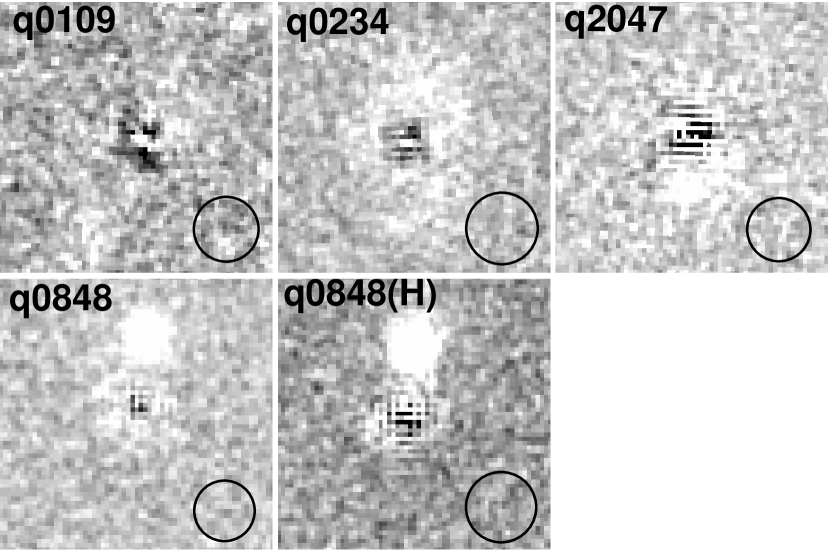
Figure 13: Closeups of likely hosts. Boxes are 4″on a side with North up, East left, and circles as in Fig. 10. Top row: NIRI targets. Bottom row: PANIC object q0848 in K and H.

For host galaxies, our detection limits are of course brighter than the limits for galaxies in the field. We inspected the radial profiles together with the two-dimensional fits to classify detections as y/?/n (likely/maybe/unlikely) with results given in Table 4. We looked for residuals that extend beyond the sizes of the circles shown in Fig. 10, and that are not likely attributable to nearby (projected on the sky) companions. We further used the 1D fits to verify that the residuals were plausibly broader than the PSF. We find four likely hosts, and note that they are seen on the images that have the best seeing, $\rm FWHM<0\farcs 4$, and nearly maximal depth, indicating that we are pushing the limits of detection with these images. Other objects might well have hosts lurking just beneath the noise. Three of the four likely detections are found on NIRI images. The fuzz associated with quasar q0848 in the Ks band was marginally detected in H as well. These four likely hosts are shown in Fig. 13.

For all of the objects observed with PANIC or NIRI, we estimate the host detection limits by applying our $D_{iso}\gtrsim 2.5~{}\rm FWHM$ criterion using the curves in Fig. 12 and the surface brightnesses and FWHMs in Table 1. The results are summarized in Table 4, where we list for each model two possible values for the limit on the host galaxy.

The “conservative” value represents the most luminous host that would be just visible; the galaxies may be luminous but are conspiring to evade detection either by putting too much light in their unresolved cores or by having such a large scale length that the middle radii are below the sky. The “optimistic” value represents the least luminous host that would be just visible. Of course the stellar masses of the galaxies in Table 4 could be considerably smaller than the straight luminosities indicate. For example, if we allow for 2 mag of evolution, then the the present-day equivalents would be galaxies lower in luminosity by a factor of $\sim 6$. In that case, a 12$\rm L^{*}$ galaxy in the Table would represent 2$\rm L^{*}$ of stellar mass.

One can see from Table 4 that for the depth and resolution of our images, the range in upper limits for each type of galaxy typically spans a factor of two. In addition, the luminosity limits for deVaucouleurs galaxies are typically double those for exponentials, reflecting the fact that the peakier spheroids can hide more light in the unresolved core. In general, the least certain limits by the isophotal diameter method will be for those images with big FWHM and/or shallow depths, because in these cases galaxy isophotal diameters are only weakly dependent on galaxy luminosity–in other words, they fall on the flat outer parts of the curves in Fig. 12b. The ClassicCam images were sufficiently insensitive that the limits are not interesting. There are also several PANIC and NIRI images whose conservative limits were so large as to be also uninteresting.

7.2 Host Detections

For the four likely hosts we can also estimate fluxes from the residuals after fitting. We use Fig. 12a first to identify the kind of galaxy that could yield the observed magnitude and isophotal diameter for the surface brightness limit of the image. We then use Fig. 12b to translate that into a possible intrinsic B-band luminosity for the whole galaxy. Note that this luminosity is bigger than the luminosity one would calculate simply from applying the distance modulus to the observed magnitude; it includes contributions from the inner part of the galaxy under the PSF and from the outer part below the sky noise. Finally, we apply 2 mag of evolution to the luminosity and from it calculate the corresponding $M_{B}$ that a galaxy of the same stellar mass would have today.

For q0109, the residuals add up to $m_{K}^{Vega}\rm(obs)\sim 22.7$ and they extend to a diameter of approximately 2$\farcs$. We use Fig. 12a (the 22.4$\rm mag~{}arcsec^{-2}$ depth is appropriate for this image) to learn that this galaxy could for example be a large scale-length exponential disk. Locating this curve on Fig. 12b, we find that the same $D_{iso}$ gives a luminosity of $\sim 30\hbox{$\rm L^{*}$}$ with no evolution. Allowing for 2 mag of evolution yields a galaxy with mass corresponding to a $\sim 5\hbox{$\rm L^{*}$}$ galaxy today. For comparison, the object at $1\farcs 5$ southeast of the quasar has $m_{K}^{Vega}\rm(obs)\sim 22.7$ and $D_{iso}\sim 1\farcs 1$. If it is at the redshift of the quasar, it could represent a companion with roughly half the mass of the host at a projected separation of about 11kpc.

For the bright residuals in q0234, we measure $D_{iso}\sim 2\farcs 6$, while integrating the 1D residuals gives $m_{K}^{Vega}\rm(obs)\sim 19.9$–bright enough to represent a $\sim 60\hbox{$\rm L^{*}$}$ exponential (10$\rm L^{*}$with evolution), again with a large scale length.

A similar analysis for q0848 gives $D_{iso}\sim 1\farcs 2$ and $m_{K}^{Vega}\rm(obs)\sim 19.4$ which could be a $\sim 24\hbox{$\rm L^{*}$}$ (4$\rm L^{*}$with evolution) disk.

For q2047, the residuals extend asymmetrically to the south and possibly represent the combined flux of the host and a companion. This object’s classification as a hyperluminous infrared galaxy by Rowan-Robinson (2000) (based on sub-mm emission that is likely too strong to originate in the quasar’s dust torus) would suggest that we are observing a merger. Integrating the 1D residuals gives $m_{K}^{Vega}\rm(obs)\sim 19.7$. The diameter is harder to define because of the asymmetry but we adopt $1\farcs 6$ as an estimate, which implies a $\sim 40\hbox{$\rm L^{*}$}$-mass, intermediate scale length exponential (7$\rm L^{*}$with evolution).

Table 4 shows that three of the four detections are more luminous than the conservative detection thresholds for exponentials and all fall above the optimistic thresholds. We overplot the estimates on Fig. 14-16.

If we examine the deVaucouleurs curves in Fig. 12 we find that the residuals for q0109 and q0234 are too big for their magnitudes observed to be represented by the curves plotted; in other words, if they are spheroids, they must have $r_{eff}>>4\rm kpc$. On the other hand, the residuals for q0848 and q2047 fall on the curves for $r_{eff}=4\rm kpc$ and could be spheroids with masses of 1-2 times their exponential counterparts.

For the several quasars with detections listed as “?” the data do not warrant any attempt to characterize the magnitudes other than to say that if the hosts are there, they likely lie close to the limits listed in Table 4.

7.3 Color of the Host Galaxy of SDSSpJ084811.52-001418.0

For one of the quasars with a detected host, SDSSpJ084811.52-001418.0, we also obtained a deep H-band image with PANIC. We carried out the PSF estimation and subtraction from the nuclear quasar image for the H-band, and found a residual flux, consistent with the K-band detection. The color of the host light is H-K=0.8. This color is nominally bluer than that of a redshifted spiral galaxy spectral energy distribution, which would have H-K=2.0. The quasar itself has H-K=0.5, as expected for a quasar at this redshift (Chiu et al., 2007).

Thus, the host galaxy is redder than the quasar itself, but bluer than a young stellar population at $z=4$. It could be that the host is experiencing a burst of star-formation, as one would expect to occur for a major merger of gas-rich galaxies, and is metal-poor, so has a weak 4000Åbreak. Another possible explanation, however, is that the host light is contaminated by a foreground galaxy. There is no known damped Ly-$\alpha$ absorber along the SDSSpJ084811.52-001418.0 sight-line (Murphy & Liske, 2004) but other intervening absorption line systems are no doubt present. Finally, we note that the uncertainty in the H-K color is very large, and difficult to estimate. Deeper imaging of a larger sample, or spectroscopy of the fuzz, could distinguish among these possibilities.

7.4 The Local Black-hole/Bulge Relation

In this section we compare our limits with the local black-hole/bulge relation. While the local relation is given for spheroids, we include both exponential and deVaucouleurs models in our discussion to allow for the possibility that the stellar mass might be differently distributed at early cosmological times. Wherever necessary we have adjusted values to our adopted cosmology, and we have transformed host absolute magnitudes in the literature to $M_{B}$ assuming galaxy rest-frame colors $B-V$=0.8, $B-R=1.4$, and $B-H=4$, all appropriate for a spiral-like stellar population. For an older (elliptical-like) population the colors are up to 0.3mag redder, but the uncertainties in these colors are small compared to the other uncertainties.

We have computed rest-frame absolute $B$ magnitude limits for our hosts from the luminosities in Table 4 assuming 2 magnitudes of evolution. We plot our host limits and black hole masses against the local relation in Fig. 14, where the local population is represented by (i) the Tremaine et al. (2002) local galaxies, (ii) the Lauer et al. (2007) local fit, and (iii) the McLure & Dunlop (2001) local ($z<0.3$) luminous quasars, the latter which provide high-mass black hole counterparts analogous to those in our sample of high-z quasars. The results are similar if we use our $0.4L_{edd}$ estimates for the black hole mass. We interpret this figure as follows. The conservative case occurs where the hosts are all at their maximum allowed values, i.e. with limit given by the right-hand bar of each pair and hiding much flux in either a very compact core or in the low surface brightness wings of a shallow profile. In this case, the exponential and deVaucouleurs distributions are both consistent with the local relation for the two magnitudes of evolution assumed; the limits thus do not provide interesting constraints on possible evolution in the relation. The optimistic case occurs when the left-hand bar in each pair gives the upper limit to the galaxy luminosity. In this case, the limits for deVaucouleurs hosts remain uninteresting. On the other hand, hosts with exponential profiles would be less massive for a given black hole mass than are the local (Tremaine) galaxies, though might yet be consistent with local quasars. However, if the evolution correction are more than the two magnitudes assumed, our optimistic exponential upper limits would yield hosts lower in mass for a given black hole mass than local luminous quasars. The Bruzual & Charlot (2003) models suggest that evolution in excess of 2 magnitudes between $z=4$ and now would be expected if for example the population were younger than about 400Myr at $z=4$.

Fig. 15 shows a similar comparison for quasars at various redshifts. The local quasar sample is the McLure & Dunlop (2001) local ($z<0.3$) used above. Intermediate-redshift objects ($z>1$) are from the Peng et al. (2006) compilation of quasars observed with HST’s NICMOS and having virial black hole mass estimates. They include 15 unlensed objects from Ridgway et al. (2001) and Kukula et al. (2001) and 36 objects (most lensed) from their own observations. The points in Fig. 15 are shown with no evolution correction, which explains the (rightward) trend towards more luminous hosts for a given black hole mass as redshift increases. Peng et al. (2006) found that an evolution correction for a passively evolving population formed at high redshift pushes the intermediate-redshift hosts leftward beyond the local relation, implying smaller stellar mass relative to the black hole mass compared to local galaxies. The constraints from our high-z objects are also dependent on the amount of evolution as discussed above.

In Fig. 16, we plot our host limits against rest-frame nuclear $B$-band absolute magnitude, and compare them to those in the $z<0.4$ quasar host galaxy compilation by McLeod & McLeod (2001). Because the observed $K_{s}$ directly traces the rest-frame $B$ for our quasars, the $B$-band absolute magnitude plotted here is independent of the nuclear spectral shape and so provides an complementary approach to using black hole mass as a tracer of the nuclear engine. We see from the plots that the limits for exponential hosts imply galaxies fainter than their low-z counterparts, especially using the optimistic limits (bottom bar in each pair) as a bright limit. The same is true for the optimistic deVaucouleurs limits. As in the previous discussion, any excess evolution would push the two distributions farther apart. An obvious limitation here is that there are few local quasars with luminosities as high as those of the $z=4$ sample. However, one solid conclusion from Fig. 16 is that there does appear to be a maximum allowed host. For the 2 mag of evolution plotted, this maximum corresponds to $M_{B}\sim-24$ in the conservative limit, or $M_{B}\sim-23$ (roughly a 10$\rm L^{*}$ galaxy) in the optimistic case. Alternatively, if there are ever independent suggestions that the mass limit must be less than that corresponding to an 10$\rm L^{*}$ galaxy, then our results would imply that the evolution must be more than the 2 mag assumed.

7.5 K-band Galaxy Evolution: The K-z relation

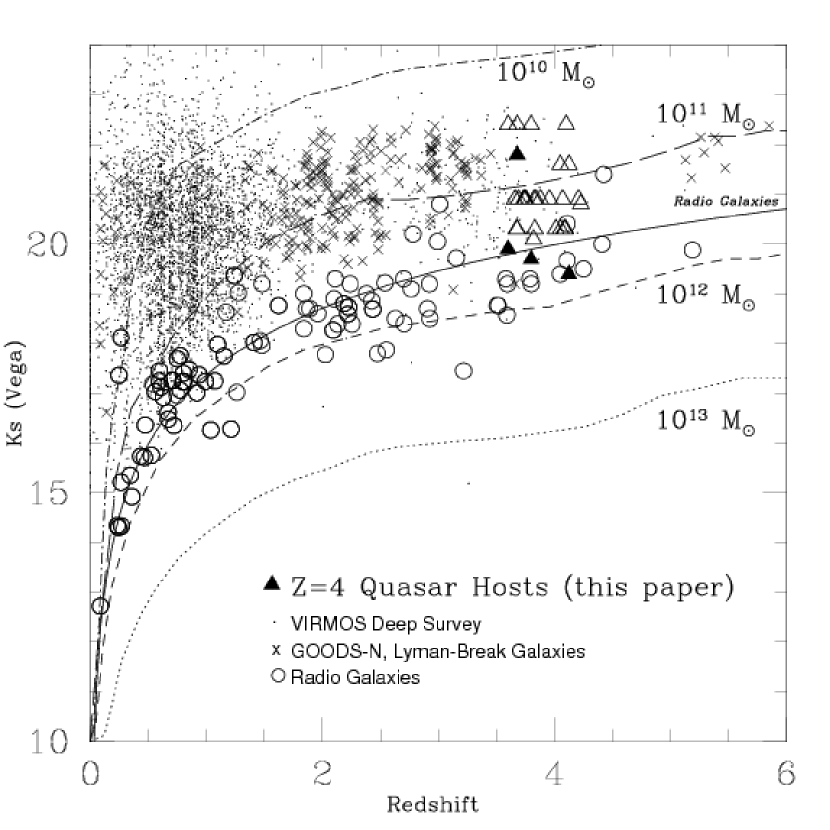
Figure 17: K-z Diagram for Radio Galaxies, Field Galaxies, and $z=4$ Quasar Hosts. The filled triangles are the four detected host galaxies of this survey; open triangles are optimistic limits listed in Table 4. Open circles are radio galaxies (Lacy et al. 2000, De Breuck et al. 2002, Willott et al 2003, De Breuck et al 2006). X’s are optically-selected galaxies (Reddy et al. 2006, McLure et al 2006), and dots are galaxies in the VIRMOS deep galaxy survey (Iovino et al. 2005, Temporin et al. 2008). The solid line is the fit to the locus of radio galaxies, as given by Willott et al. (2003). The dotted, dashed, long-dashed and dot-dashed lines are evolutionary tracks for elliptical galaxies of mass 10${}^{13}M_{\sun}$, 10${}^{12}M_{\sun}$,10${}^{11}M_{\sun}$, and 10${}^{10}M_{\sun}$, respectively, as computed by Rocca-Volmerange et al. (2004). All magnitudes are $K_{s}$ in the Vega system. The detected quasar hosts have $K_{s}$ magnitudes consistent with those of massive galaxies at their redshifts.

To look at our observations another way, we plot $K_{s}$-magnitude versus redshift in Figure 17. The observed $K_{s}$-magnitude of a given galaxy varies with redshift because of k-corrections, evolution of the galaxy’s stellar population, and merging. Here we compare the quasar host galaxies of our study with observations of the $K_{s}$-magnitude of field galaxies at the same redshift.

We plot observed $K_{s}$-magnitudes for radio galaxies (Lacy et al., 2000; De Breuck et al., 2002; Willott et al., 2003; De Breuck et al., 2006), which define the locus of brightest galaxies at all redshifts. The locus of radio galaxies is plotted as a solid line given by

$$K_{s}=17.37+4.53log_{10}z-0.31(log_{10}z)^{2}$$

from Willott et al. (2003). Fainter galaxies found as Lyman dropouts (Reddy et al., 2006) or similar optical selection (Iovino et al., 2005; McLure et al., 2006; Temporin et al., 2008) and subsequent spectroscopic redshift measurement are shown as well. We plot Vega magnitudes for $K_{s}$, and convert from $K_{AB}$ given in the literature by assuming that $K_{AB}=K_{Vega}+{1.84}$. The sharp locus of the radio galaxies is interpreted to indicate a maximum mass for galaxies of $10^{12}\rm M_{\sun}$, possibly the result of a fragmentation limit in cooling proto-galactic gas clouds. Also shown are the expected $K_{s}$-band evolution tracks for elliptical galaxies of various masses as computed by Rocca-Volmerange et al. (2004). The evolution curves for spirals are similar (see Rocca-Volmerange et al. (2004)). We see that between $z=0.25$ and $z=4$, we expect a given mass galaxy to undergo approximately 5 magnitudes of evolution at $K_{s}$.

Note that of the four z=4 hosts detected here, three (SDSS010905.8+001617.1, SDSSpJ023446.58-001415.9, and PC2047+0123) are radio quiet. The other, SDSSpJ084811.52-001418.0, lacks definitive radio data. Despite having radio quiet nuclei, two of the three most luminous hosts have magnitudes comparable to those of radio galaxies at the same redshift.

If we interpret the host galaxy detections with the Rocca-Volmerange et al. (2004) model for spheroids in the K-z diagram, then we can derive the ratio of black hole mass to spheroid mass: we find a ratio of 0.016, compared to the local value of $1.4\pm 0.4\times 10^{-3}$ seen locally (Häring & Rix, 2004). In other words, given the black hole masses we inferred from the emission lines, the local relation would imply more massive host galaxies than we see. This is what is predicted by theory (Croton, 2006; Somerville et al., 2008).

7.6 Malmquist Bias in This Sample

Lauer et al. (2007) have emphasized that surveys of high redshift quasars suffer from such strong Malmquist bias that drawing conclusions about the evolution of host galaxies from small samples is problematic. The problem is that we pick targets based on their quasar luminosity, then look for the host. Even if there is a correlation between host galaxy luminosity and black hole luminosity, the observed host galaxies will be systematically fainter than the mean relation derived from spheroid velocity dispersions. This is because for any plausible galaxy luminosity function, there are many more faint galaxies than bright ones. Thus the intrinsic scatter in the relation causes an excess of low-luminosity galaxies with black holes big enough to make the sample.

To look at this effect quantitatively for our sample, we carried out a Monte-Carlo simulation. We chose galaxies randomly from a Schechter galaxy luminosity function, from L/ $\rm L^{*}$= 0.1 to 15, given by

$$\phi(L)dL={{n_{*}}(L/\hbox{$\rm L^{*}$})^{\alpha}exp(-L/\hbox{$\rm L^{*}$})}dL/\hbox{$\rm L^{*}$}$$

with $\alpha=-0.46$, and $\hbox{$\rm L^{*}$}=2\times 10^{10}L_{\odot}$ (Sparke & Gallagher, 2007). We assume a galaxy mass-to-light ratio M/L=5 (Cappellari et al., 2006; Tortora et al., 2009), so that the corresponding mass of an $\rm L^{*}$ galaxy is M*$\approx 10^{11}M_{\odot}$. Then, we assign to each galaxy a black hole with mass chosen randomly from the Häring & Rix (2004) distribution, in which black holes have mass 0.14% +/-0.04% of the galaxy mass. We further assume that to be found as a luminous quasar and be eligible for inclusion in our sample, the object must have a black hole mass above a certain cutoff, taken to be either $\rm log_{10}(M_{BH}/M_{\odot})=8.5$ or $9.0$. We draw millions of galaxies, and count up the fraction of host galaxies as a function of host galaxy luminosity for all objects with black hole masses above our threshold. The results are shown in Fig. 18.

As expected, we see that for a given value of the black hole cutoff mass, the results will be skewed towards lower-luminosity hosts than inferred from the mean value of the black hole-bulge relation. If we take a cutoff of $\rm log_{10}(M_{BH}/M_{\odot})=8.5$, which is at the small end of our sample, the effect is modest; most of the hosts would be very close to the expected mean value of about 2$\rm L^{*}$. However, if we restrict our sample to the more massive black holes, $\rm log_{10}(M_{BH}/M_{\odot})=9$, the effect is somewhat larger with the bulk of the contributors in the range 4-8$\rm L^{*}$, skewed from the expected mean value of 7$\rm L^{*}$. However, even if we include the effects of the Malquist bias, we could have detected such hosts for the most massive black holes in our sample, those with $\rm log_{10}(M_{BH}/M_{\odot})>9.5$, if the evolution were at least two magnitudes as discussed above.

8 Discussion

When we initiated this program, we hoped to test whether or not quasars at $z=4$ followed the same correlation of black-hole mass and host galaxy spheroid mass seen in spheroids locally. We knew in principle that if the very luminous nuclei in the high redshift objects were hosted by proportionately massive spheroids, they would be relatively straight-forward to detect at K, with the best ground-based seeing. We have taken a very conservative approach to reducing the data, to looking for host galaxy detections, and to estimating host galaxy fluxes and limits.

We explored more than one way to compare our observed detection of hosts and limits on host galaxies to the low redshift spheroids. This comparison is complicated for a number of reasons, primarily the fact that we do not measure spheroid velocity dispersion or mass directly, but must infer the host galaxy properties from the emitted starlight. Nonetheless, our data indicate that the host galaxies of some z=4 quasars in our sample are fainter than we expect from the low-redshift correlations.

We note that for the mean local values $M_{BH}/M_{gal}=0.14\%$ and M/L=5, we expect black holes with $\rm log_{10}(M_{BH}/M_{\odot})=9.5,10,\rm~{}and~{}10.5$, to have host galaxies with $M_{gal}=2,7,\rm~{}and~{}22x10^{12}\hbox{$\rm M_{\odot}$}$, or $L/\hbox{$\rm L^{*}$}=20,70,\rm~{}and~{}220$ respectively. However, such galaxies are implausibly large, and do not have present-day analogues. For example, as shown in Fig. 17, the upper mass envelope for radio galaxies corresponds to $10^{12}\hbox{$\rm M_{\odot}$}$, or $L\approx 10\hbox{$\rm L^{*}$}$. This suggests that the $M_{BH}/M_{gal}$ correlation must plateau at $M_{gal}\approx 10^{12}\hbox{$\rm M_{\odot}$}$.

9 Summary

We observed 34 high redshift quasars in the near-IR to search for their host galaxies. Our conclusions are the following.

1. We found that to characterize the PSF and subtract the nuclear quasar light properly, we had to account for geometric distortions in the camera optics, and non-linearity in the detectors, beyond what is normally corrected for in standard pipeline reductions. We caution that small uncertainties in the linearity correction, and the use of PSF stars which are significantly brighter than the quasar, can lead to undersubtraction of the nuclear PSF, and spurious host galaxy detections.

2. We derived black hole masses for the quasars in the sample from the profile of the C IV emission line, but noted several cases where the profile appears to include a narrow and broad component. Low signal-to-noise spectra could easily miss the broad component, with the result that the black hole mass is underestimated. The black hole masses range from $10^{8.7}$ to $10^{10.7}\hbox{$\rm M_{\odot}$}$. These quasars are very luminous, and so rare as to be not represented in some models for quasar evolution (e.g. Kauffmann & Haehnelt (2000); Di Matteo et al. (2008)). They are more luminous than the knee in the quasar luminosity function, and are probably peak emitters (Hopkins et al., 2008) that are undergoing a major merger.

3. Accretion rates were derived from the observed K photometry, which directly samples the rest-frame B for the sample quasars. The median accretion rate of the sample corresponds to an Eddington fraction of $L_{bol}/L_{Edd}=0.41\pm 0.3$, consistent with the findings for other samples such as the Sloan quasars, and for low redshift quasars whose host galaxies have been studied by a number of authors.

4. We estimated the K-band magnitudes of the host galaxies of the quasars in our sample with a new method which takes into account the isophotal diameter of the galaxies as a function of redshift, as well as the surface brightness limit of the images. We explored parameter space by considering galaxies with exponential and deVaucouleur radial light distributions, and quantified the dependance of derived host galaxy properties on assumed galaxy properties.

5. We detected host galaxies for 4 quasars, at least three of which are radio quiet.The detections all occurred on our deepest, sharpest images. The K-band luminosities of the hosts are consistent with massive galaxies at the redshifts of the quasars. For one object with H-band data, the K-H color is bluer than expected for a star-forming galaxy at the quasar redshift, but the uncertainties in the color are large.

6. We interpreted the detected hosts and limits on host luminosity in several ways, taking into account expected evolution of the stellar populations. We find that if the hosts are already spheroids at early times, then their black-hole/bulge relation could well be consistent with that for local galaxies and luminous quasars; our limits are weak in the case of very compact or very extended spheroids. On the other hand, if the hosts are exponential disks, they likely have less stellar mass for a given black hole mass than would be inferred from the extrapolation of the local relation to high black hole masses, but they could contain as much stellar mass as the spheroidal component of local luminous quasars. Any $B$-band rest frame luminosity evolution in excess of the 2 magnitudes assumed would make any evolution in the black-hole/bulge relation stronger; such would be the case for a stellar population younger than $\sim$400Myr.

7. If we interpret the K-magnitudes of the detected hosts with models for the evolution of massive spheroids we find that the ratio of black hole mass to spheroid mass for the 4 detected hosts is approximately 0.02, compared to $1.4\pm 0.4\times 10^{-3}$ observed in local spheroids. Several authors have pointed out that the Malmquist bias inherent in any study that looks for hosts in very luminous, rare quasars will overestimate the black hole mass to spheroid ratio, given the likely scatter in the correlations, and the fact that faint galaxies outnumber bright ones. We made a rough estimate of the Malmquist bias in our sample through a Monte Carlo simulation. We find that our detection rate is inconsistent with what we should have seen, had the z=4 quasars followed the same relation between black-hole mass and spheroid mass. Instead, the host galaxies in the past appear fainter (and by assumption less massive) than host galaxies today. This conclusion depends on uncertain assumptions for the scatter in the black-hole mass-spheroid correlation, the mass-to-light ratios of galaxies, and the evolution of the spectral energy distribution of spheroids. However, our results are in broad agreement with semi-analytical models for the growth of black holes and merger-induced activity.

Figure 1: Magnitude and redshift distribution for the 34 quasars observed here (squares) and quasars from the Sloan Quasar Catalog (Schneider et al. , 2007).

Figure 2: New Keck DEIMOS spectra of five quasars in the region around CIV in the rest-frame used for estimating black hole masses. The spectrum for [VH]2125-4529 also provided an improved redshift.

Figure 3: Black hole masses as a function of z for the 34 quasars observed here (filled squares) shown on top of those determined for $\approx 1600$ SDSS quasars in this redshift range by Shen et al. (2008). For several objects the CIV line profile shows a distinct broad component whose FWHM yields black hole masses (open squares) an order of magnitude larger than the overall FWHM would indicate.

Figure 7: Nonlinearity data for PANIC camera based on exposures of internal calibration lamps with three possible prescriptions for linearity corrections. Exposure times are generally chosen to keep quasars (and PSF stars) below about 15,000 ADU. At this level the possible corrections vary by $\lesssim 0.5\%$.

Figure 9: Radial profiles for the simulated stars described in §5.2 and shown in Fig. 8. The stars that have not been corrected for linearity. For p40, whose flux puts it into the nonlinear regime, the profile is obviously different. For p10 and p1, the more subtle nonlinearity falsely suggests a host contribution in the profile, though the residuals are unphysically compact.

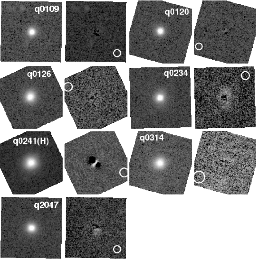
Figure 10: Closeups of quasars (left image in each pair) and residuals after PSF fits, $\sim 8\arcsec$ on a side for targets observed with NIRI. Images are shown with North up, East to the left. The circles have diameter $D=2.5\rm FWHM$. The obviously bad fit for q0241H resulted from telescope mirror support problems, and illustrates the effects of distortion in an extreme case. The q0120 image shows the much more subtle but typical effect of residual distortion and nonlinearity. In the case of q0234, significant residuals are obvious.

Figure 10 cont’d–targets observed with PANIC. In most cases the fit to the core is excellent.

Figure 10 cont’d–targets observed with PANIC.

Figure 10 cont’d–targets observed with PANIC.

Figure 10 cont’d–targets observed with ClassicCam. Fits are generally poorer than those for NIRI and PANIC. As described in the text, for the small ClassicCam field of view, PSF stars were not visible on the same frames as the quasar and had to be obtained in separate observations interleaved with the quasar exposures. In addition, the ClassicCam images generally have broader PSFs and shallower depths.

Figure 11: Radial profiles labeled with instrument names (C1,C2=ClassicCam, N=NIRI, P=PANIC). Quasar data points are plotted with standard-of-the-mean errors. PSFs are shown as solid lines normalized to the central pixel. Dotted lines show positive parts of residuals after subtraction. Vertical bars mark the radius corresponding to a diameter as $D=2.5\rm FWHM$ discussed in the text.

Fig. 11 cont’d.

Figure 12: Isophotal diameter predictions v. observed magnitude $m_{K_{s}}^{Vega}\rm(obs)$ (a) and luminosity $L/L^{*}$ (b) for model galaxies at $z=4$. The observed magnitudes include only the galaxy flux that is inside the isophotal diameter. The luminosity plots assume no evolution; with a more realistic 2 magnitudes of evolution the luminosity axis labels will decrease by a factor of $\sim 6$. The quantity $r$ represents $r_{0}$ and $r_{eff}$ for exponential and deVaucouleurs laws respectively. The three vertical panels in each set represent surface brightness limits appropriate for the range of our NIRI/PANIC observations. Dashed horizontal lines show the median FWHM and $2.5~{}\rm FWHM$. As described in §6.2, we set detection limits for the various host galaxy types according to the criterion $D_{iso}\gtrsim 2.5~{}\rm FWHM$.

Figure 14: Comparison with the local black-hole/bulge relation. Local galaxies are represented by the open circles from Tremaine et al. (2002) plus the diagonal line fit from Lauer et al. (2007). Local luminous quasars from McLure & Dunlop (2001) are shown as filled squares. For each of our objects, the two connected vertical bars mark the optimistic (left end) and conservative (right end) upper limits on luminosity for the range of galaxy scale lengths represented in Fig. 12. Limits are plotted for (a) exponential hosts and (b) deVaucouleurs hosts. Triangles indicate the host luminosity estimates for the 4 host galaxies detected. Our host magnitudes and limits have been corrected for 2 mag of evolution. Data from ClassicCam are not plotted, for clarity. All values from the literature have been adjusted to $H_{0}=70\rm~{}km~{}s^{-1}~{}Mpc^{-1}$.

Figure 15: Comparison with quasars at different redshifts. Local luminous quasars (filled squares) and the diagonal line are the same as in Fig. 14. Intermediate redshift quasars from the Peng et al. (2006) compilation are shown as circles. For each of our objects, limits are plotted as in Fig. 14 except that here we have made no correction for evolution. Data from ClassicCam are not plotted, for clarity.

Figure 16: Nuclear absolute magnitude v. galaxy magnitude. Squares show local quasars from the compilation of McLeod & McLeod (2001) adjusted to $H_{0}=70\rm~{}km~{}s^{-1}~{}Mpc^{-1}$. For each of our high-z quasars, the two vertical bars mark the optimistic (bottom end) and conservative (top end) absolute magnitude limits for the range of galaxy scale lengths represented in Fig. 12 and assuming 2 magnitudes of evolution. Triangles indicate the four detected hosts at z=4. For clarity, the data from ClassicCam are not plotted.

Figure 18: Results of Monte Carlo simulation of Malmquist bias for M/L=5. Curves represent the fraction of bright galaxies at each luminosity expected to have black hole masses above the cutoff value shown when drawn at random from a Schechter function and assigned a black hole mass according to the present-day Magorrian relation and its scatter. The vertical bars show the corresponding galaxy mass predicted from the Magorrian relation with no scatter. For the bigger cutoff black hole mass, the Malmquist bias is more severe, in that there is a larger contribution from galaxies with lower-luminosities than that inferred from Magorrian relation mean.

Table 1: Sample and Observations

							Time	FWHM	SBlim
Name	z	$\rm r_{AB}$	ref	Date	Inst	Filter	(min)	(″)	$mag/^{\prime\prime 2}$
SDSSpJ010905.81+001617.1	3.680	20.50	Fan01,SS	2003 Sep 11	N	Ks	250	0.35	22.62
SDSSJ012019.99+000735.5	4.101	19.96	SS	2003 Nov 05	N	Ks	125	0.32	22.41
SDSSpJ012650.77+011611.8	3.660	19.20	Fan99	2003 Nov 03	N	Ks	125	0.41	22.36
SDSSpJ023446.58-001415.9	3.600	20.17	Fan01,SS	2003 Sep 12	N	Ks	245	0.39	22.64
BRI0241-0146	4.053	18.50	SL96,ACS	2005 Jan 26-27	P	Ks	143	0.55	21.67
BRI0241-0146	4.053	18.50	SL96,ACS	2003 Sep 10	N	H	219	0.45	23.28
BRJ0301-5537	4.133	19.20	P01	2002 Sep 22	C1	Ks	108	0.82	20.84
BRJ0311-1722	4.039	18.30	P01	2002 Sep 21	C1	Ks	129	0.38	20.83
SDSSpJ031427.92+002339.4	3.680	20.55	Fan01,SS	2003 Nov 06	N	Ks	125	0.57	22.30
SDSSpJ032226.10-055824.7	3.957	20.07	SS	2004 Jan 05	P	Ks	135	0.41	21.76
SDSSpJ034109.35-064805.1	4.070	20.48	SS	2004 Jan 04	P	Ks	135	0.41	21.95
BR0401-1711	4.227	19.60	P01	2005 Jan 28	P	Ks	94	0.43	21.58
SDSSpJ040550.26+005931.2	4.050	20.22	Fan01	2004 Jan 02	P	Ks	128	0.35	21.81
BRJ0529-3552	4.172	18.80	P01	2003 Jan 20	C2	Ks	108	0.42	20.45
PMNJ0741-5305	3.743	21.90	L01	2004 Jan 06	P	Ks	135	0.47	21.87
SDSSpJ084455.08+001848.5	3.690	19.90	S01,SS	2004 Jan 05	P	Ks	142	0.45	21.78
SDSSpJ084811.52-001418.0	4.124	19.24	SS	2004 Jan 02	P	Ks	162	0.36	21.98
SDSSpJ084811.52-001418.0	4.124	19.24	SS	2004 Jan 04	P	Hc	199	0.41	22.82
SDSSpJ085430.18+004213.6	4.084	20.29	SS	2004 Jan 03	P	Ks	155	0.50	21.70
SDSSJ094822.97+005554.3	3.878	20.30	SS	2004 Mar 09	P	Ks	196	0.39	22.00
SDSSJ094822.97+005554.3	3.878	20.30	SS	2005 Jan 28	P	Hc	203	0.70	22.81
SDSSJ095755.63-002027.5	3.753	19.36	SS	2005 Jan 26	P	Ks	250	0.46	22.16
SDSSJ095755.63-002027.5	3.753	19.36	SS	2005 Jan 27	P	Hc	202	0.42	22.32
SDSSJ100151.58-001627.0	3.674	19.31	SS	2004 Mar 11	P	Ks	169	0.57	21.85
SDSSpJ101832.46+001436.4	3.826	20.22	SS	2004 Mar 10	P	Ks	209	0.40	21.87
SDSSpJ102043.82+000105.8	4.207	20.53	SS	2004 Mar 08	P	Ks	182	0.43	21.88
SDSSJ135134.46-003652.2	4.010	20.13	SS	2004 Mar 11	P	Ks	209	0.51	21.92
SDSSJ151618.44-000544.1	3.735	20.23	SS	2004 Mar 08	P	Ks	148	0.41	21.86
SDSSpJ152443.19+011358.9	4.095	20.14	SDSS2	2003 Jul 17-18	P	Ks	213	0.58	21.67
SDSSpJ154014.57+001854.7	3.830	20.41	S01,SS	2004 Mar 10	P	Ks	169	0.50	21.89
SDSSpJ161926.87-011825.2	3.840	20.17	Fan00	2004 Mar 09	P	Ks	155	0.44	21.90
SDSSpJ165527.61-000619.2	3.990	20.05	Fan00	2003 Jul 19	P	Ks	157	0.64	21.67
[HB89]2000-330	3.773	17.6	HB,WFPC2	2002 Sep 22	C1	Ks	117	0.82	20.72
PC2047+0123	3.799	19.46	S91	2003 Sep 10-11	N	Ks	154	0.35	22.46
[VH95]2125-4529	3.763	19.50	HV96	2003 Jul 18	P	Ks	146	0.56	21.54
[VCV96]Q2133-4625	4.180	21.23	VV,HV96	2003 Jul 17	P	Ks	243	0.66	21.84
BR2212-1626	3.990	18.80	SL96	2002 Sep 21	C1	Ks	117	0.42	20.69
BR2212-1626	3.990	18.80	SL96	2003 Jul 19	P	Hc	157	0.57	21.89
BRJ2317-4345	3.943	18.80	P01	2002 Sep 20	C1	Ks	117	0.46	20.69

Table 2: Radio Properties

					$F_{1.4GHz}$				RL or
Name	z	E(B-V)	$i^{AB}$	i ref	(mJy)	Flux ref	t	R $(2\sigma)$	RQ?
SDSSpJ010905.81+001617.1	3.680	0.026	20.31	SS	$<$ 0.110	FIRST	18.80	0.90	Q
SDSSJ012019.99+000735.5	4.101	0.037	19.82	SS	$<$ 0.112	FIRST	18.78	0.72	Q
SDSSpJ012650.77+011611.8	3.660	0.026	19.17	Fan99	0.210	C01	18.09	0.43	Q
SDSSpJ023446.58-001415.9	3.600	0.022	19.88	SS	$<$ 0.108	FIRST	18.82	0.73	Q
BRI0241-0146	4.053	0.028	18.24	ACS	$<$ 0.150	FIRST	18.46	0.13	Q
BRJ0301-5537	4.133	0.010	18.97	P01	…	[NED]	…	…	?
BRJ0311-1722	4.039	0.032	18.01	P01	$<$ 2.500	NVSS	15.41	1.34	?
SDSSpJ031427.92+002339.4	3.680	0.100	20.04	SS	$<$ 0.112	FIRST	18.78	0.81	Q
SDSSpJ032226.10-055824.7	3.957	0.053	19.86	SS	$<$ 2.500	NVSS	15.41	2.08	?
SDSSpJ034109.35-064805.1	4.070	0.053	20.09	SS	$<$ 2.500	NVSS	15.41	2.17	?
BR0401-1711	4.227	0.026	19.33	P01	$<$ 2.500	NVSS	15.41	1.87	?
SDSSpJ040550.26+005931.2	4.050	0.444	19.08	Fan01	$<$ 2.500	NVSS	15.41	1.77	?
BRJ0529-3552	4.172	0.031	18.51	P01	$<$ 2.500	NVSS	15.41	1.54	?
PMNJ0741-5305	3.743	0.227	21.08	L01	44.000	G93	12.29	3.51	L
SDSSpJ084455.08+001848.5	3.690	0.035	19.74	SS	5.830	NVSS	14.49	2.10	L
SDSSpJ084811.52-001418.0	4.124	0.030	18.93	SS	$<$ 2.500	NVSS	15.41	1.71	?
SDSSpJ085430.18+004213.6	4.084	0.049	19.84	SS	$<$ 2.500	NVSS	15.41	2.07	?
SDSSJ094822.97+005554.3	3.878	0.109	19.85	SS	2.320	FIRST	15.49	1.75	L
SDSSJ095755.63-002027.5	3.753	0.033	19.28	SS	$<$ 0.149	FIRST	18.47	0.63	Q
SDSSJ100151.58-001627.0	3.674	0.037	19.18	SS	$<$ 0.146	FIRST	18.49	0.58	Q
SDSSpJ101832.46+001436.4	3.826	0.043	19.98	SS	$<$ 0.151	FIRST	18.45	0.91	Q
SDSSpJ102043.82+000105.8	4.207	0.040	19.75	SS	2.000	FIRSTc	15.65	1.64	L
SDSSJ135134.46-003652.2	4.010	0.034	19.79	SS	$<$ 0.148	FIRST	18.47	0.83	Q
SDSSJ151618.44-000544.1	3.735	0.057	19.89	SS	$<$ 0.045	C01	19.77	0.35	Q
SDSSpJ152443.19+011358.9	4.095	0.055	19.88	SS	$<$ 0.143	FIRST	18.51	0.85	Q
SDSSpJ154014.57+001854.7	3.830	0.092	20.06	SS	$<$ 0.151	FIRST	18.45	0.94	Q
SDSSpJ161926.87-011825.2	3.840	0.117	19.69	Fan00	$<$ 0.025	C01	20.41	0.01	Q
SDSSpJ165527.61-000619.2	3.990	0.298	19.54	Fan00	0.010	C01	21.40	-0.74	Q
[HB89]2000-330	3.773	0.130	17.04	WFPC2	570.00	W90	9.51	3.01	L
PC2047+0123	3.799	0.105	19.07	S91	0.105	S92	18.85	0.09	Q
[VH95]2125-4529	3.763	0.022	19.15	HV96	…	[NED]	…	…	?
[VCV96]Q2133-4625	4.180	0.025	21.04	HV96	…	[NED]	…	…	?
BR2212-1626	3.990	0.028	18.49	SL96	$<$ 2.500	NVSS	15.41	1.54	?
BRJ2317-4345	3.943	0.011	18.57	P01	…	[NED]	…	…	?

Table 3: Black Hole Properties

				$\rm FWHM_{CIV}$			$\rm M_{BH}$	$L_{bol}/L_{Edd}$	$\rm M_{BH}$
Name	z	$\rm AB_{1450}$	AB ref	($km~{}s^{-1}$)	CIV ref	$M_{B}^{Vega}$	CIV	CIV	$0.4L_{Edd}$
SDSSpJ010905.81+001617.1	3.680	20.89	Fan01	4980	Fan01	-25.5	9.1	0.40	9.0
SDSSJ012019.99+000735.5	4.101	19.96	Fan01	4840	SS	-26.7	9.3	0.69	9.4
SDSSpJ012650.77+011611.8	3.660	19.58	Fan99	3991/8756	Fan99	-26.6	9.2/9.8	0.89/0.19	9.4
SDSSpJ023446.58-001415.9	3.600	20.40	S01	3030	SS	-26.1	8.7	1.45	9.2
BRI0241-0146	4.053	18.23	i	9552	C02	-28.3	10.2	0.34	10.1
BRJ0301-5537	4.133	18.97	i	6728	P01	-27.3	9.8	0.39	9.7
BRJ0311-1722	4.039	18.00	i	15117	P01	-28.5	10.7	0.15	10.2
SDSSpJ031427.92+002339.4	3.680	20.33	Fan01	3758	SS	-25.9	8.9	0.74	9.1
SDSSpJ032226.10-055824.7	3.957	20.21	SS	7100	SS	-26.5	9.6	0.33	9.4
SDSSpJ034109.35-064805.1	4.070	20.70	SS	7033	SS	-26.0	9.5	0.25	9.2
BR0401-1711	4.227	19.34	i	2004/5504	C02	-27.8	8.7/9.5	7.83/1.04	9.9
SDSSpJ040550.26+005931.2	4.050	19.27	Fan01	3070	Fan01	-27.1	9.0	1.83	9.6
BRJ0529-3552	4.172	18.52	i	3210	P01	-27.9	9.2	2.40	9.9
PMNJ0741-5305	3.743	21.04	i	9990	L01	-26.9	9.7	0.37	9.5
SDSSpJ084455.08+001848.5	3.690	20.05	S01	1752/8605	Keck	-25.7	8.3/9.7	2.4/0.1	9.0
SDSSpJ084811.52-001418.0	4.124	18.93	SS	5371	Keck	-27.3	9.6	0.62	9.7
SDSSpJ085430.18+004213.6	4.084	20.10	SS	5580	Keck	-26.5	9.4	0.49	9.4
SDSSJ094822.97+005554.3	3.878	21.05	SS	6078	SS	-26.4	9.2	0.58	9.3
SDSSJ095755.63-002027.5	3.753	20.10	SS	4964	SS	-27.1	9.2	1.15	9.6
SDSSJ100151.58-001627.0	3.674	20.08	SS	6813	SS	-26.8	9.5	0.47	9.5
SDSSpJ101832.46+001436.4	3.826	20.19	S01	5657	SS	-26.3	9.3	0.44	9.3
SDSSpJ102043.82+000105.8	4.207	20.35	SS	8847	SS	-27.4	9.7	0.46	9.7
SDSSJ135134.46-003652.2	4.010	20.74	SS	5420	SS	-26.9	9.2	0.98	9.5
SDSSJ151618.44-000544.1	3.735	20.10	Fan00	10631	SS	-26.1	9.9	0.10	9.2
SDSSpJ152443.19+011358.9	4.095	20.73	SS	10228	SS	-26.9	9.8	0.28	9.5
SDSSpJ154014.57+001854.7	3.830	20.20	S01	9707	S01	-26.0	9.8	0.11	9.1
SDSSpJ161926.87-011825.2	3.840	20.04	Fan00	6076	Fan00	-25.8	9.4	0.22	9.1
SDSSpJ165527.61-000619.2	3.990	20.22	Fan00	3102/12181	Fan00	-27.2	8.8/10.0	3.21/0.21	9.6
[HB89]2000-330	3.773	17.01	i	4081	K01	-28.7	9.7	1.55	10.2
PC2047+0123	3.799	19.23	S92	6316	Keck	-27.4	9.6	0.58	9.7
[VH95]2125-4529	3.763	19.12	i	6257	Keck	-26.6	9.7	0.28	9.4
[VCV96]Q2133-4625	4.180	21.04	D03	…	…	-25.5	…	…	8.9
BR2212-1626	3.990	18.52	SL96	2739/6185	C02	-28.5	9.1/9.8	5.59/1.10	10.1
BRJ2317-4345	3.943	18.55	i	4612	P01	-27.4	9.5	0.79	9.7

Table 4: Results from $K_{s}$ Imaging

			$L_{exp}/\hbox{$\rm L^{*}$}$		$L_{deV}/\hbox{$\rm L^{*}$}$					$L_{host}/\hbox{$\rm L^{*}$}$
Name	z	$K_{s,quasar}^{Vega}$	min	max	min	max	$K_{s,min}^{Vega}$	Host	$K_{s,host}^{Vega}$	no ev	ev	$M_{B,host}^{Vega}$
SDSSpJ010905.81+001617.1	3.680	18.3	9	14	15	19	21.40	y	21.8	30	5	-22.2
SDSSJ012019.99+000735.5	4.101	17.5	7	14	15	15	21.80	n	…	…	…	…
SDSSpJ012650.77+011611.8	3.660	17.1	24	42	42	72	19.90	?n	…	…	…	…
SDSSpJ023446.58-001415.9	3.600	17.6	9	15	19	24	20.80	y	19.9	60	10	-23.0
BRI0241-0146	4.053	15.9	53	130	92	140	18.40	n	…	…	…	…
BRI0241-0146	4.053	16.5	…	…	…	…	…	n	…	…	…	…
BRJ0301-5537	4.133	16.9	…	…	…	…	…	n	…	…	…	…
BRJ0311-1722	4.039	15.6	…	…	…	…	…	n	…	…	…	…
SDSSpJ031427.92+002339.4	3.680	17.9	53	130	92	140	18.40	n	…	…	…	…
SDSSpJ032226.10-055824.7	3.957	17.5	24	42	42	72	19.90	n	…	…	…	…
SDSSpJ034109.35-064805.1	4.070	18.2	24	42	42	72	19.90	?n	…	…	…	…
BR0401-1711	4.227	16.5	42	53	72	91	19.60	n	…	…	…	…
SDSSpJ040550.26+005931.2	4.050	17.0	19	32	32	42	20.60	n	…	…	…	…
BRJ0529-3552	4.172	16.3	…	…	…	…	…	n	…	…	…	…
PMNJ0741-5305	3.743	16.9	32	53	53	91	19.40	n	…	…	…	…
SDSSpJ084455.08+001848.5	3.690	18.1	32	53	53	91	19.40	n	…	…	…	…
SDSSpJ084811.52-001418.0	4.124	16.9	19	32	33	42	20.30	y	19.4	24	4	-22.0
SDSSpJ084811.52-001418.0	4.124	17.4	…	…	…	…	…	y?	…	…	…	…
SDSSpJ085430.18+004213.6	4.084	17.6	42	72	72	130	19.00	n	…	…	…	…
SDSSJ094822.97+005554.3	3.878	17.6	24	42	42	53	19.90	n	…	…	…	…
SDSSJ094822.97+005554.3	3.878	18.2	…	…	…	…	…	n	…	…	…	…
SDSSJ095755.63-002027.5	3.753	16.7	32	53	53	91	19.40	n	…	…	…	…
SDSSJ095755.63-002027.5	3.753	17.5	…	…	…	…	…	n	…	…	…	…
SDSSJ100151.58-001627.0	3.674	17.0	53	130	92	140	18.40	n	…	…	…	…
SDSSpJ101832.46+001436.4	3.826	17.6	24	42	42	72	19.90	n	…	…	…	…
SDSSpJ102043.82+000105.8	4.207	16.9	32	42	53	72	19.60	n	…	…	…	…
SDSSJ135134.46-003652.2	4.010	17.2	42	92	72	130	18.70	n	…	…	…	…
SDSSJ151618.44-000544.1	3.735	17.8	24	42	42	72	19.90	n	…	…	…	…
SDSSpJ152443.19+011358.9	4.095	17.3	53	140	92	…	18.20	n	…	…	…	…
SDSSpJ154014.57+001854.7	3.830	18.0	42	72	72	130	19.00	y?	…	…	…	…
SDSSpJ161926.87-011825.2	3.840	18.1	32	42	53	72	19.60	n	…	…	…	…
SDSSpJ165527.61-000619.2	3.990	16.9	71	…	130	…	18.80	n	…	…	…	…
[HB89]2000-330	3.773	15.2	…	…	…	…	…	n	…	…	…	…
PC2047+0123	3.799	16.5	9	14	15	19	21.40	y	19.7	40	7	-22.6
[VH95]2125-4529	3.763	17.3	71	130	130	…	18.40	n	…	…	…	…
[VCV96]Q2133-4625	4.180	18.8	71	…	130	…	18.40	n	…	…	…	…
BR2212-1626	3.990	15.6	…	…	…	…	…	n	…	…	…	…
BR2212-1626	3.990	16.3	…	…	…	…	…	n	…	…	…	…
BRJ2317-4345	3.943	16.6	…	…	…	…	…	n	…	…	…	…

References

- Ammons et al. (2009) Ammons, S.M., Melbourne, J., Max, C.E., Koo, D.C., & Rosario, D.J.V. 2009, AJ, 137, 470.
- Aretxaga, Terlevich, & Boyle (1998) Aretxaga, I., Terlevich, R. J., & Boyle, B. J. 1998, MNRAS, 296, 643.
- Aretxaga et al. (1998) Aretxaga, I., Le Mignant, D., Melnick, J., Terlevich, R. J., & Boyle, B. J. 1998, MNRAS, 298, L13.
- Bechtold & McLeod (2009) Bechtold, J., & McLeod, K. 2009, Paper II, in prep.
- Becker et al. (1995) Becker, R. H., White, R. L., & Helfand, D. J. 1995, ApJ, 450, 559
- Bruzual & Charlot (2003) Bruzual, G., & Charlot, S. 2003, MNRAS, 344, 1000
- Cappellari et al. (2006) Cappellari, M., et al. 2006, MNRAS, 366, 1126
- Carballo et al. (1998) Carballo, R., Sánchez, S. F., González-Serrano, J. I., Benn, C. R., & Vigotti, M. 1998, AJ, 115, 1234.
- Carilli et al. (2001) Carilli, C. L., et al. 2001, ApJ, 555, 625.
- Chiu et al. (2007) Chiu, K., Richards, G. T., Hewett, P. C., & Maddox, N. 2007, MNRAS, 375, 1180
- Collin et al. (2002) Collin, S., Boisson, C., Mouchet, M., Dumont, A.-M., Coupé, S., Porquet, D., & Rokaki, E. 2002, A&A, 388, 771
- Condon et al. (1998) Condon, J. J., Cotton, W. D., Greisen, E. W., Yin, Q. F., Perley, R. A., Taylor, G. B., & Broderick, J. J. 1998, AJ, 115, 1693
- Constantin et al. (2002) Constantin, A., Shields, J. C., Hamann, F., Foltz, C. B., & Chaffee, F. H. 2002, ApJ, 565, 50.
- Croom et al. (2004) Croom, S. M., Schade, D., Boyle, B. J., Shanks, T., Miller, L., & Smith, R. J. 2004, ApJ, 606, 126.
- Croton (2006) Croton, D. J. 2006, MNRAS, 369, 1808
- Davis et al. (2003) Davis, M., et al. 2003, Proc. SPIE, 4834, 161
- De Breuck et al. (2002) De Breuck, C., van Breugel, W., Stanford, S. A., Röttgering, H., Miley, G., & Stern, D. 2002, AJ, 123, 637
- De Breuck et al. (2006) De Breuck, C., Klamer, I., Johnston, H., Hunstead, R. W., Bryant, J., Rocca-Volmerange, B., & Sadler, E. M. 2006, MNRAS, 366, 58
- Dietrich & Hamann (2004) Dietrich, M., & Hamann, F. 2004, ApJ, 611, 761
- Dietrich et al. (2003) Dietrich, M., Appenzeller, I., Hamann, F., Heidt, J., Jäger, K., Vestergaard, M., & Wagner, S. J. 2003, A&A, 398, 891
- Di Matteo et al. (2008) Di Matteo, T., Colberg, J., Springel, V., Hernquist, L., & Sijacki, D. 2008, ApJ, 676, 33
- Elmegreen et al. (2007) Elmegreen, D. M., Elmegreen, B. G., Ravindranath, S., & Coe, D. A. 2007, ApJ, 658, 763
- Elvis et al. (1994) Elvis, M., et al. 1994, ApJS, 95, 1
- Falomo et al. (2008) Falomo, R., Treves, A., Kotilainen, J. K., Scarpa, R., & Uslenghi, M. 2008, ApJ, 673, 694
- Fan et al. (1999) Fan, X., et al. 1999, AJ, 118, 1
- Fan et al. (2000) Fan, X., et al. 2000, AJ, 119, 1
- Fan et al. (2001) Fan, X., et al. 2001, AJ, 121, 31
- Ferrarese & Merritt (2000) Ferrarese, L., & Merritt, D. 2000, ApJ, 539, L9.
- Floyd et al. (2004) Floyd, D. J. et al. 2004, MNRAS, 355, 196.
- Gebhardt et al. (2000) Gebhardt, K., et al. 2000, ApJ, 539, L13.
- Griffith & Wright (1993) Griffith, M. R., & Wright, A. E. 1993, AJ, 105, 1666.
- Häring & Rix (2004) Häring, N., & Rix, H.-W. 2004, ApJ, 604, L89
- Hawkins & Veron (1996) Hawkins, M.R.S. & Veron, P. 1996, MNRAS, 281, 348.
- Hewitt & Burbidge (1989) Hewitt, A., & Burbidge, G. 1989, ApJS, 69, 1.
- Hodapp, K. W. et al. (2003) Hodapp et al. 2003, PASP, 115, 1388.
- Hopkins et al. (2005) Hopkins, P. F., Hernquist, L., Cox, T. J., Di Matteo, T., Martini, P., Robertson, B., & Springel, V. 2005, ApJ, 630, 705
- Hopkins et al. (2008) Hopkins, P. F., Hernquist, L., Cox, T. J., & Kereš, D. 2008, ApJS, 175, 356
- Hutchings et al. (1999) Hutchings, J. B., Crampton, D., Morris, S. L., Durand, D., & Steinbring, E. 1999, AJ, 117, 1109.
- Hutchings (2003) Hutchings, J. B. 2003, AJ, 125, 1053.
- Hutchings (2005) Hutchings, J. B. 2005, PASP, 117, 1250.
- Iovino et al. (2005) Iovino, A., et al. 2005, A&A, 442, 423
- Ivezic et al. (2002) Ivezic, Z. et al. 2002, AJ, 124, 2364.
- Jiang et al. (2007) Jiang, L.et al. 2007, ApJ, 656, 680.
- Kaspi et al. (2005) Kaspi, S., Maoz, D., Netzer, H., Peterson, B. M., Vestergaard, M., & Jannuzi, B. T. 2005, ApJ, 629, 61
- Kauffmann & Haehnelt (2000) Kauffmann, G. & Haehnelt, M. 2000, MNRAS, 311, 576.
- Kauffmann & Haehnelt (2002) Kauffmann, G. & Haehnelt, M. 2002, MNRAS, 332, 529.
- Kelly & Bechtold (2007) Kelly, B. C., & Bechtold, J. 2007, ApJS, 168, 1
- Kelly et al. (2008) Kelly, B. C., Bechtold, J., Trump, J. R., Vestergaard, M., & Siemiginowska, A. 2008, ApJS, 176, 355
- Kim et al. (2008) Kim, M., Ho, L. C., Peng, C. Y., Barth, A. J., & Im, M. 2008,ApJS,197,283
- Kiuchi et al. (2009) Kiuchi, G., Ohta, K.,& Akiyama, M. 2009, ApJ, 696, 1051
- Kormendy & Richstone (1995) Kormendy, J., & Richstone, D. 1995, ARA&A, 33, 581.
- Kuhlbrodt et al. (2005) Kuhlbrodt, B., Orndahl, E., Wisotzki, L., & Jahnke, K. 2005, A&A, 439, 497.
- Kuhn et al. (2001) Kuhn, O. et al. 2001, ApJS, 136, 225.
- Kukula et al. (2001) Kukula, M. J., Dunlop, J. S., McLure, R. J., Miller, L., Percival, W. J., Baum, S. A., & O’Dea, C. P. 2001,MNRAS, 326, 1533.
- Lacy et al. (2000) Lacy, M., Bunker, A. J., & Ridgway, S. E. 2000, AJ, 120, 68
- Landt et al. (2001) Landt, H., Padovani, P., Perlman, E. S., Giommi, P., Bignall, H., & Tzioumis, A. 2001, MNRAS, 323, 757.
- Lauer et al. (2007) Lauer, T. R., Tremaine, S., Richstone, D., and Faber, S.M. 2007, ApJ,670, 249.
- Lehár et al. (2000) Lehár, J., et al. 2000, ApJ, 536, 584.
- Lehnert et al. (1992) Lehnert, M. D., Heckman, T. M., Chambers, K. C., & Miley, G. K. 1992, ApJ, 393, 68.
- Lowenthal et al. (1995) Lowenthal, J. D., Heckman, T. M., Lehnert, M. D., & Elias, J. H. 1995, ApJ, 439, 588.
- Magorrian et al. (1998) M agorrian, J., et al. 1998. AJ, 115, 2285.
- Marconi & Hunt (2003) Marconi, A., & Hunt, L. K. 2003, ApJ, 589, L21.
- Martini et al. (2004) Martini, P., Persson, S.E. Murphy, D.C., Birk, C., Shectman, S.A., Gunnels, S.M., & Koch, E. 2004, Proc. SPIE, 5492, 1653
- McGill et al. (2008) McGill, K. L., Woo, J.-H., Treu, T., & Malkan, M. A. 2008, ApJ, 673, 703
- McLeod & Rieke (1995) McLeod, K. K., & Rieke, G. H. 1995, ApJ, 454, L77.
- McLeod, Rieke, & Storrie-Lombardi (1999) McLeod, K. K., Rieke, G. H., & Storrie-Lombardi, L. J. 1999, ApJ, 511, L67.
- McLeod & McLeod (2001) McLeod, K. K. & McLeod, B. A. 2001, ApJ, 546, 782.
- McLure et al. (1999) McLure, R. J., Kukula, M. J., Dunlop, J. S., Baum, S. A., O’Dea, C. P., & Hughes, D. H. 1999, MNRAS, 308, 377.
- McLure & Dunlop (2001) McLure, R. J., & Dunlop, J. S. 2001, MNRAS, 327, 199.
- McLure et al. (2006) McLure, R. J., et al. 2006, MNRAS, 372, 357
- Mo & White (2002) Mo, H. J., & White, S. D. M. 2002, MNRAS, 336, 112.
- Murphy & Liske (2004) Murphy, M. T., & Liske, J. 2004, MNRAS, 354, L31
- Netzer et al. (2007) Netzer, H., Lira, P., Trakhtenbrot, B., Shemmer, O., & Cury, I. 2007, ApJ, 671, 1256
- Oke & Gunn (1983) Oke, J.B. & Gunn, J.E. 1983, ApJ, 266, 713.
- Peng et al. (2006) Peng, C. Y., et al. 2006, ApJ, 649, 616.
- Pentericci et al. (2003) Pentericci, L. et al. 2003, A&A, 410, 75.
- Péroux et al. (2001) Péroux, C., Storrie-Lombardi, L. J., McMahon, R. G., Irwin, M., & Hook, I. M. 2001, AJ, 121, 1799.
- Persson et al. (1998) Persson, S. E., Murphy, D. C, Krzeminski, W., Roth, M., & Rieke, M. J. 1998, AJ, 116, 2475.
- Persson et al. (1992) Persson, S. E., West, S. C., Carr, D. M., Sivaramakrishnan, A., & Murphy, D. C. 1992, PASP, 104, 204.
- Peterson et al. (2004) Peterson, B. M., et al. 2004, ApJ, 13, 682
- Reddy et al. (2006) Reddy, N. A., Steidel, C. C., Erb, D. K., Shapley, A. E., & Pettini, M. 2006, ApJ, 653, 1004
- Ridgway et al. (2001) Ridgway, S., Heckman, T., Calzetti, D., & Lehnert, M. 2001, ApJ, 550, 122.
- Rocca-Volmerange et al. (2004) Rocca-Volmerange, B., Le Borgne, D., De Breuck, C., Fioc, M., & Moy, E. 2004, A&A, 415, 931.
- Rowan-Robinson (2000) Rowan-Robinson, M. 2000, MNRAS, 316, 885
- Saracco et al. (2006) Saracco, P. et al. 2006, MNRAS, 367, 349.
- Schlegel et al. (1998) Schlegel, D.J., Finkbeiner, D.P., & Davis, M. et al. 1998, ApJ, 500, 525.
- Schneider et al. (1991) Schneider, D. P., Schmidt, M., & Gunn, J. E. 1991, AJ, 101, 2004.
- Schneider et al. (1992) Schneider, D. P., van Gorkom, J. H., Schmidt, M., & Gunn, J. E. 1992, AJ, 103, 1451.
- Schneider et al. (2001) Schneider, D. P., et al. . 2001, AJ, 121, 1232.
- Schneider et al. (2003) Schneider, D. P. et al. 2003, AJ, 126, 2579.
- Schneider et al. (2007) Schneider, D. P. et al. 2007, AJ, 134, 102.
- Shen et al. (2008) Shen, Y., Greene, J. E., Strauss, M. A., Richards, G. T., & Schneider, D. P. 2008, ApJ, 680, 169.
- Silverman et al. (2009) Silverman, J. D., et al. 2009, ApJ, 696, 396
- Somerville et al. (2008) Somerville, R. S., Hopkins, P. F., Cox, T. J., Robertson, B. E., Hernquist, L. 2008, MNRAS, 391, 481
- Sparke & Gallagher (2007) Sparke, L. S., & Gallagher, J. S., III 2007, Galaxies in the Universe: An Introduction. Second Edition. By Linda S. Sparke and John S. Gallagher, III. ISBN-13 978-0-521-85593-8 (HB); ISBN-13 978-0-521-67186-6 (PB). Published by Cambridge University Press, Cambridge, UK.
- Storrie-Lombardi et al. (1996) Storrie-Lombardi, L. J., McMahon, R. G., Irwin, M. J., & Hazard, C. 1996, ApJ, 468, 121.
- Storrie-Lombardi & Wolfe (2000) Storrie-Lombardi, L. J., & Wolfe, A. M. 2000, ApJ, 543, 552.
- Temporin et al. (2008) Temporin, S., et al. 2008, A&A, 482, 81, accessed through http://cencosw.oamp.fr/En/VVDS-DEEP/
- Tortora et al. (2009) Tortora, C., Napolitano, N. R., Romanowsky, A. J., Capaccioli, M., & Covone, G. 2009, MNRAS, 396, 1132
- Tremaine et al. (2002) Tremaine, S., et al. 2002, ApJ, 574, 740.
- Treu et al. (2007) Treu, T., Woo, J.-H., Malkan, M. A., & Blandford, R. D. 2007, ApJ, 667, 117
- VandenBerk et al. (2001) VandenBerk, D.E. et al. 2001, AJ, 122, 549.
- Véron-Cetty & Véron (1996) Véron-Cetty, M.-P., & Véron, P. 1996, ESO Scientific Report (7th ed; Garching: ESO), c1996
- Véron-Cetty & Véron (2001) Véron-Cetty, M.-P., & Véron, P. 2001, A&A, 374, 92.
- Vestergaard & Peterson (2006) Vestergaard, M., & Peterson, B. M. 2006, ApJ, 641, 689.
- Wandel et al. (1999) Wandel, A., Peterson, B. M., & Malkan, M. A. 1999, ApJ, 526, 579
- Warren et al. (2001) Warren, S. J., Møller, P., Fall, S. M., & Jakobsen, P. 2001, MNRAS, 326, 759
- Weedman (1986) Weedman, D. W. 1986, Quasar Astronomy, (Cambridge U. Press)
- Willott et al. (2003) Willott, C. J., Rawlings, S., Jarvis, M. J., & Blundell, K. M. 2003, MNRAS, 339, 173
- Woo et al. (2008) Woo, J.-H., Treu, T., Malkan, M. A., & Blandford, R. D. 2008, ApJ, 681, 925
- Wright & Otrupcek (1990) Wright, A., & Otrupcek, R. 1990, PKS Catalog (1990), 0.