Strong nonlocality: A trade-off between states and measurements

Abstract

Measurements on entangled quantum states can produce outcomes that are nonlocally correlated. But according to Tsirelson’s theorem, there is a quantitative limit on quantum nonlocality. It is interesting to explore what would happen if Tsirelson’s bound were violated. To this end, we consider a model that allows arbitrary nonlocal correlations, colloquially referred to as “box world”. We show that while box world allows more highly entangled states than quantum theory, measurements in box world are rather limited. As a consequence there is no entanglement swapping, teleportation or dense coding.

I Introduction

Despite its great explanatory and predictive power, the standard formalism of quantum theory - in which states are represented by vectors in a complex Hilbert space - retains an abstract mathematical character. Of course there is no reason why Nature should not be described by an abstract mathematical formalism. But it is notable that in quantum theory textbooks, the formalism is simply postulated. It is not, say, derived from a small set of elementary physical considerations in the manner of special relativity. This invites the question: why that structure, as opposed to any other?

One way to approach this question, or at least gain some insight, is to compare and contrast quantum theory with other models - theoretical possibilities which do not describe our universe, but which can nonetheless be explored. In this paper, we investigate one particular non-classical, non-quantum theory. In barrett , this theory was called generalized non-signalling theory, or GNST for short, as it admits all non-signalling correlations popescu ; boxes . Here we call it box world.

One of the notable features of box world is that, as in quantum theory, measurements on separate but entangled systems can produce outcomes that are nonlocally correlated, i.e., which cannot be explained by any local hidden-variable model bell ; CHSH . It is already known that nonlocal correlations are useful in many information theoretic tasks qi1 ; qi2 . But in quantum theory, there is a quantitative limit on the amount of nonlocality that correlations can have tsirelson . In box world, by contrast, arbitrary nonlocal correlations can be produced, as long as they do not permit instantaneous signalling. This has consequences. For example, with stronger than quantum correlations, it is known that communication complexity problems become trivial, requiring only constant communication van-dam ; brassardetal . On the other hand, as we show in this paper, possibilities for measurement in box world are in some ways rather limited. It turns out that there is nothing analogous to a Bell measurement. We also show that there is no entanglement swapping, teleportation, or dense coding. This extends to the whole of box world previous special-case results in barrett ; coupler .

As entanglement swapping is possible in the quantum world swapping , it follows that box world does not contain quantum theory as a special case, and that it cannot be the true theory describing reality.

II A framework for probabilistic theories

In order to compare classical theories, quantum theories, and alternatives such as box world, we need a common mathematical framework in which the different theories can be written down. We begin by describing such a framework. It is operational in flavour. This means, for example, that system, preparation and measurement are all taken as basic terms. Different ways of preparing a system will prepare different states. The state of a system determines the outcome probabilities for any measurement that can be performed on the system. The framework we describe and the notation we use is closely based on that of lucien and barrett . However, we should note that there is nothing very novel in the framework itself, and that numerous formalisms have been developed over the years, intended to be operational generalizations of classical and quantum theory (see e.g., lucien ; dariano ; convex1 ; convex2 ).

II.1 Single systems

One way of specifying the state of a system would be to give an exhaustive list of the outcome probabilities for every possible measurement. However, as Hardy points out lucien , most physical theories have enough structure that it is not necessary to give such an exhaustive list in order to specify the state fully. Instead, for each type of system, assume that its state can be completely characterised by the outcome probabilities for some finite subset of all possible measurements. Following Hardy, we refer to the subset chosen to represent the state as fiducial measurements. If the outcome probabilities for the fiducial measurements are known, then the state is known, and the outcome probabilities for any other measurement can be inferred. For example, the state of a single qubit in quantum theory corresponds to a density operator on a 2-dimensional Hilbert space. But equally, it can be completely characterised by the outcome probabilities of measurements corresponding to the three Pauli operators, $\sigma_{x},\sigma_{y}$ and $\sigma_{z}$. Note that the choice of which measurements to use as fiducial measurements is not unique.

A convenient way of writing down the state is as a vector $\mathbf{P}$, with components $P(a|x)$, where this is the probability of obtaining outcome $a$ when fiducial measurement $x$ is performed. Obviously, $P(a|x)$ must be positive and normalised such that $\sum_{a}P(a|x)=1$. For example, for binary valued $a$ and $x$:

$$\mathbf{P}=\left(\begin{array}[]{c}P(0|0)\\ P(1|0)\\ \hline\cr P(0|1)\\ P(1|1)\end{array}\right).$$ (1)

Within a particular operational model, it is not necessarily the case that any vector $\mathbf{P}$ represents an allowed state (that is, a state which can actually be prepared). In quantum theory there is no qubit state that assigns probability 1 to the +1 outcome for all three Pauli measurements. An operational model must specify, for each type of system, a set $\mathcal{P}$ of states which can physically be prepared. We assume that arbitrary probabilistic mixtures of states can be prepared (e.g., by tossing some coins and preparing either state $\mathbf{P}$ or state $\mathbf{Q}$ depending on the result). Hence $\mathcal{P}$ is convex.

II.2 Multi-partite systems

Most of the interesting questions that can be asked in information theory involve more than one system. So how should we describe the state of a multi-partite system in a general operational model? Consider $n$ systems, $A_{1},\ldots,A_{n}$, with a set of fiducial measurements for each. If a fiducial measurement $x_{1}$ is performed on $A_{1}$, $x_{2}$ on $A_{2}$, and so on, then at the least, the joint state of $A_{1},\ldots,A_{n}$ should determine a joint probability for each combination of outcomes. We assume something further: a specification of the joint probability of each combination of outcomes for each possible combination of fiducial measurements is sufficient to determine completely the joint state. Note that this property does indeed hold in both quantum theory and classical probability theory. But it is not trivial. For example, in an alternative quantum theory, formulated using real instead of complex Hilbert spaces, the property does not hold realqm1 ; realqm2 ; realqm3 .

It is convenient to write a multi-partite state of $n$ systems in the form of an $n$-dimensional array, with entries $P(\mathbf{a}|\mathbf{x})$, where $\mathbf{x}=(x_{1},\ldots,x_{n})$ specifies a fiducial measurement for each subsystem, $\mathbf{a}$ is a list of the corresponding measurement outcomes, and $P(\mathbf{a}|\mathbf{x})$ is the probability of getting $\mathbf{a}$ given $\mathbf{x}$. For example, for two systems, each with a binary measurement choice $x$, and binary outcomes $a$:

$$\mathbf{P}=\left(\begin{array}[]{cc|cc}P(00|00)&P(01|00)&P(00|01)&P(01|01)\\ P(10|00)&P(11|00)&P(10|01)&P(11|01)\\ \hline\cr P(00|10)&P(01|10)&P(00|11)&P(01|11)\\ P(10|10)&P(11|10)&P(10|11)&P(11|11)\end{array}\right)$$ (2)

Conditions of positivity and normalisation apply as before.

Finally, all multi-partite states must satisfy the no-signalling conditions:

$\sum_{a_{n}}P(\mathbf{a}|\mathbf{x})$   is independent of $x_{n}$ for all $n$.

These ensure that separated parties cannot send messages to one another simply by making measurements on their subsystems. Arguably, if the no-signalling conditions do not hold, then we had no right to be speaking of separate subsystems in the first place.

A multi-partite state is a product state if $\mathbf{P}$ satisfies

$$P(\mathbf{a}|\mathbf{x})=P_{1}(a_{1}|x_{1})P_{2}(a_{2}|x_{2})\ldots P_{n}(a_{n}|x_{n}),$$ (3)

where $P_{i}(a_{i}|x_{i})$ is a valid state of the $i$th system. A state is separable if it can be written as a convex combination of product states, otherwise it is entangled.

II.3 Measurements

In general, the fiducial measurements will not be the only measurements that one can perform on a system. For example, on a single qubit, there is a measurement corresponding to $\sigma_{45^{\circ}}=1/\sqrt{2}(\sigma_{x}+\sigma_{z})$. On two qubits there is a Bell measurement. By the definition of the fiducial measurements, it must be possible to derive the measurement probabilities for all such measurements from the $P(\mathbf{a}|\mathbf{x})$.

In fact, by considering mixtures of states, it can be shown that the probability $\mathrm{Pr}(r)$ of obtaining a particular outcome $r$ in any measurement must be a linear function of the fiducial measurement probabilities lucien ; barrett . We can therefore associate an effect $\mathbf{R}_{r}$ with each measurement outcome, where $\mathbf{R}_{r}$ is an array with components $R_{r}(\mathbf{a}|\mathbf{x})$, such that

$$\mathrm{Pr}(r)=\mathbf{R_{r}}\cdot\mathbf{P}\equiv\sum_{\mathbf{ax}}R_{r}(\mathbf{a}|\mathbf{x})P(\mathbf{a}|\mathbf{x}).$$ (4)

A measurement with various possible outcomes is associated with a set $\{\mathbf{R}_{r}\}$. For example, consider again a qubit in quantum theory, with fiducial measurements chosen to be $\sigma_{x},\sigma_{y},\sigma_{z}$. The measurement corresponding to $\sigma_{45^{\circ}}$ is represented by the $1$-dimensional arrays

$$\mathbf{R}_{+1}=\left(\begin{array}[]{r}2^{-\frac{3}{2}}\\ -2^{-\frac{3}{2}}\\ \hline\cr 2^{-1}\\ 2^{-1}\\ \hline\cr 2^{-\frac{3}{2}}\\ -2^{-\frac{3}{2}}\end{array}\right),\ \ \ \mathbf{R}_{-1}=\left(\begin{array}[]{r}-2^{-\frac{3}{2}}\\ 2^{-\frac{3}{2}}\\ \hline\cr 2^{-1}\\ 2^{-1}\\ \hline\cr-2^{-\frac{3}{2}}\\ 2^{-\frac{3}{2}}\end{array}\right)$$ (5)

Note that the array $\mathbf{R}_{r}$ associated with a measurement outcome is not in general unique, since there may be a different array $\mathbf{R}^{\prime}_{r}$ satisfying $\mathbf{R}_{r}\cdot\mathbf{P}=\mathbf{R}^{\prime}_{r}\cdot\mathbf{P}\;\forall\,\mathbf{P}\in\mathcal{P}$.

A particular operational model must contain a specification of the set of measurements that can physically be performed on a particular type of system. There is a constraint: any measurement must correspond to a set $\{\mathbf{R}_{r}\}$ such that

$$\mathbf{R}_{r}\cdot\mathbf{P}\geq 0\ \ \forall r\ \forall\,\mathbf{P}\in\mathcal{P}$$ (6)

and

$$\sum_{r}\mathbf{R}_{r}\cdot\mathbf{P}=1\ \ \forall\,\mathbf{P}\in\mathcal{P}.$$ (7)

Furthermore, if a measurement is performed on one subsystem of a bipartite system, it is possible to calculate the subsequent (“collapsed”) state of the other subsystem, conditioned on a particular outcome. Clearly this should be an allowed state of that subsystem.

II.4 Dynamics

In addition to preparations and measurements, it may be possible to perform transformations on a system, i.e., to act on it in such a way that the system is preserved but its state changes. In the most general case, a system can change into a system of a different type. But here we consider only transformations that preserve the type of system. Such a transformation can be represented as a map $\mathbf{T}:\mathcal{P}\rightarrow\mathcal{P}$. As with measurements, a consideration of mixed states implies that $\mathbf{T}$ is linear. Thus a transformation can be represented by an array such that

$$P^{\prime}(\mathbf{a}^{\prime}|\mathbf{x}^{\prime})=\sum_{\mathbf{ax}}T(\mathbf{a}^{\prime}|\mathbf{x}^{\prime},\mathbf{a}|\mathbf{x})P(\mathbf{a}|\mathbf{x}).$$ (8)

For each type of system, an operational model should specify a set of physically possible transformations. A valid transformation should satisfy

$$\mathbf{T}(\mathbf{P})\in\mathcal{P}\ \forall\mathbf{P}\in\mathcal{P}.$$ (9)

There are other consistency conditions that the sets of allowed states, measurements and transformations should satisfy, which we will not go into in detail. For example, if a transformation is followed by a fiducial measurement, then this process taken as a whole should correspond to a valid measurement on the initial state.

III Box World

Box world is one particular operational model, which has a natural definition in terms of the framework defined above, and which it is interesting to compare with the quantum and classical theories. Box world is defined as follows. Any $\mathbf{P}$ satisfying:

1. Positivity: $P(\mathbf{a}|\mathbf{x})\geq 0$

2. Normalisation: $|\mathbf{P}|=\sum_{\mathbf{a}}P(\mathbf{a}|\mathbf{0})=1$

3. No-signalling: $\sum_{a_{n}}P(\mathbf{a}|\mathbf{x})$ is independent of $x_{n}$

is an allowed state.

Two subtleties: first, the normalisation condition is only stated for the measurement choice $\mathbf{x}=\mathbf{0}$. But the no-signalling conditions are then sufficient to ensure normalisation for all measurement choices since they imply

$$\sum_{\mathbf{a}}P(\mathbf{a}|\mathbf{x})=\sum_{\mathbf{a}}P(\mathbf{a}|\mathbf{x^{\prime}}).$$ (10)

Second, although the no-signalling conditions refer only to fiducial measurements, it can be shown that they are sufficient to prevent signalling using any kind of measurement barrett .

Box world permits many states that do not have counterparts in quantum theory. An interesting example is this bipartite state:

$$P_{PR}(a_{1}a_{2}|x_{1}x_{2})=\left\{\begin{array}[]{ccl}\frac{1}{2}&:&a_{1}+a_{2}=x_{1}x_{2}\;\textrm{(mod 2)}\\ 0&:&\mathrm{otherwise}\end{array}\right.,$$ (11)

where $x_{1},x_{2},a_{1},a_{2}\in\{0,1\}$. The correlations generated by performing fiducial measurements on this state are nonlocal, meaning that they violate the Clauser-Horne-Shimony-Holt (CHSH) inequality CHSH . In fact, they are more nonlocal than is possible in quantum theory, because they return a value of 4 for the CHSH expression. Tsirelson’s theorem tsirelson shows that quantum correlations always return a value $\leq 2\sqrt{2}$, and CHSH showed that local correlations always return a value $\leq 2$. These superquantum nonlocal correlations have appeared in the literature before popescu ; boxes , and they are sometimes referred to as a Popescu-Rohrlich (PR) box. Thus we refer to this state as the PR box state.

What are the allowed measurements in box world? The model is defined so that any set $\{\mathbf{R}_{r}\}$ satisfying conditions (6) and (7) above corresponds to a physically possible measurement. In the following, we explore what kinds of measurement this actually allows, and the consequences for information processing. Intuitively, the fact that conditions (6) and (7) must be satisfied means that there is a tradeoff between states and measurements. If there is a larger space of states, then there is a smaller set of measurements that are compatible with those states. The space of states in box world is in an obvious sense maximal, so one would expect the possibilities for measurement to be less interesting than in, say, quantum theory. This is indeed the case.

IV Measurements in box world

The following property of measurements in box world is proven in Appendix D of barrett .

Theorem 1

All effects in box world can be represented using only positive arrays where each component satisfies

$$0\leq R(\mathbf{a}|\mathbf{x})\leq 1.$$ (12)

From hereon, assume that effects are indeed represented this way.

In the case of multi-partite systems, we have already defined product states, and distinguished separable and entangled states. Similar definitions apply to effects. A multi-partite effect is a product effect if

$$R(\mathbf{a}|\mathbf{x})=R_{1}(a_{1}|x_{1})R_{2}(a_{2}|x_{2})\ldots R_{n}(a_{n}|x_{n}),$$

where $R_{i}(a_{i}|x_{i})$ is a valid effect on the $i$th system. An effect is separable if it can be written as a sum of product effects, otherwise it is entangled. (Note that the sum here really is just a sum - not a convex combination, as in the definitions applicable to states.) Any array $\mathbf{R}$ with one entry $\in(0,1]$ and the rest zero represents a product effect. Hence Theorem 1 yields

Corollary 1

There are no entangled effects in box world.

Section VI shows that Theorem 1 also prevents entanglement swapping and teleportation in box world.

A certain class of measurements is particularly simple and will play a special role in what follows.

Definition 1

A measurement is basic if it can be implemented by a sequence of fiducial measurements on individual subsystems, where later measurement choices may depend (deterministically) on earlier outcomes, and the final measurement outcome $r$ is given by a deterministic function of the fiducial measurement outcomes $\mathbf{a}$.

An example of a basic measurement for two subsystems is given in Figure 1, where fiducial measurement $x_{1}=0$ is performed on the first subsystem and then measurement $x_{2}=a_{1}$ is performed on the second, and the final measurement outcome is given by $r=a_{2}$.

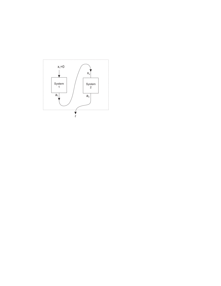
Figure 1: An example of a basic measurement on two systems, each with $x,a\in\{0,1\}$.

In general, it is reasonable to require that measurements of this form are in the set of allowed measurements in an operational model. In fact, as we can also choose such basic measurements at random, it is also reasonable to require that convex combinations of basic measurements (defined in an obvious way) are allowed. Note that for a single system, each basic measurement corresponds to a fiducial measurement, possibly with relabelled outputs.

Theorem 2

All valid measurements on single or bipartite systems in box world are convex combinations of basic measurements.

This means that any measurement on a single or bipartite system can be implemented by a probabilistic protocol involving only fiducial measurements. Especially given Corollary 1, it would be natural to assume that Theorem 2 generalises to multi-partite systems in box world, and indeed this was hypothesized in Ref. barrett . However, things are not so simple.

Theorem 3

For tri-partite systems, there are measurements which do not reduce to a convex combination of basic measurements.

Section V.2 illustrates this with a specific example.

Finally, there is at least some limitation on the power of measurements in box world, even in the multi-partite case.

Theorem 4

For any single or multi-partite system, all allowed measurements can be simulated using fiducial measurements and post-selection (i.e., the measurement is allowed to sometimes fail).

V Proofs

Some preliminary remarks will be useful. First, recall Theorem 1, which states that the entries of an effect $\mathbf{R}$ can be assumed non-negative. This is used throughout this section.

Now consider the arrays $\mathbf{R}_{r}$ corresponding to the outcomes of a basic measurement. Suppose that a basic measurement is carried out, with final outcome $r$, and that during its execution, the fiducial measurements $\mathbf{x}$ are performed, with outcomes $\mathbf{a}$. In this case, say that the triple $\{r,\mathbf{a},\mathbf{x}\}$ is realized. A basic measurement can be represented such that the component $R_{r}(\mathbf{a}|\mathbf{x})$ is equal to 1 if and only if it is possible for $\{r,\mathbf{a},\mathbf{x}\}$ to be realized, else it is 0. From hereon we make this choice. For example, the bipartite measurement illustrated in Fig. 1 is represented by

$$R_{0}(a_{1}a_{2}|x_{1}x_{2}) = \left(\begin{array}[]{c|c}\begin{array}[]{cc}1&0\\ 0&0\end{array}&\begin{array}[]{cc}0&0\\ 1&0\end{array}\\ \hline\cr\begin{array}[]{cc}0&0\\ 0&0\end{array}&\begin{array}[]{cc}0&0\\ 0&0\end{array}\end{array}\right),$$ (23)

$$R_{1}(a_{1}a_{2}|x_{1}x_{2}) = \left(\begin{array}[]{c|c}\begin{array}[]{cc}0&1\\ 0&0\end{array}&\begin{array}[]{cc}0&0\\ 0&1\end{array}\\ \hline\cr\begin{array}[]{cc}0&0\\ 0&0\end{array}&\begin{array}[]{cc}0&0\\ 0&0\end{array}\end{array}\right).$$ (34)

Definition 2

The total measurement array for a measurement $\{\mathbf{R}_{r}\}$ is given by

$$\mathbf{M}=\sum_{r}\mathbf{R}_{r}.$$ (35)

From Eq. (7), $\mathbf{M}$ satisfies

$$\mathbf{M}\cdot\mathbf{P}=1\ \ \forall\mathbf{P}\in\mathcal{P}.$$ (36)

Now consider the total measurement array corresponding to a basic measurement. It has a simple form, which can be described iteratively. First, since each $\mathbf{a}$ corresponds to a specific $r$, the component $M(\mathbf{a}|\mathbf{x})$ is equal to 1 if and only if it is possible for the pair $\{\mathbf{a},\mathbf{x}\}$ to be realized. The probability of $\{\mathbf{a},\mathbf{x}\}$ being realized is given by

$$\mathrm{Pr}(\mathbf{a},\mathbf{x})=M(\mathbf{a}|\mathbf{x})\times P(\mathbf{a}|\mathbf{x}).$$ (37)

Now, for a single system, $M(a|x)=\delta_{xi}$ for some $i$. For a multi-partite system composed of $n$ subsystems, there must exist some $k$, and some $i$, such that the first step in the basic measurement is to perform the fiducial measurement $x_{k}=i$ on the $k$th subsystem. Let $\mathbf{\hat{x}}_{k}$ represent a sequence of measurements and $\mathbf{\hat{a}}_{k}$ a sequence of outcomes on the remaining $n-1$ subsystems. $\mathbf{M}$ satisfies

$$M(\mathbf{a}|(x_{k}\neq i)\mathbf{\hat{x}}_{k})=0.$$ (38)

Define a new $(n-1)$-dimensional array $\mathbf{M}_{a_{k}}$ such that

$$M_{a_{k}}(\mathbf{\hat{a}}_{k}|\mathbf{\hat{x}}_{k})\equiv M(a_{k}\mathbf{\hat{a}}_{k}|(x_{k}=i)\mathbf{\hat{x}}_{k}).$$ (39)

For all $a_{k}$, $\mathbf{M}_{a_{k}}$ must correspond to a valid basic measurement on $(n-1)$ subsystems.

Finally, with a suitable choice of deterministic function of $\mathbf{a}$ for the output $r$, $M(\mathbf{a}|\mathbf{x})$ (consisting of 0s and 1s) can be decomposed into any sum of arrays $R_{r}(\mathbf{a}|\mathbf{x})$ (also consisting of 0s and 1s). For the measurement of Figure 1, outcomes are represented by $R_{0}$ and $R_{1}$ as in Eqs. (23) and (34), and $\mathbf{M}$ is given by

$$M(a_{1}a_{2}|x_{1}x_{2})=\left(\begin{array}[]{c|c}\begin{array}[]{cc}1&1\\ 0&0\end{array}&\begin{array}[]{cc}0&0\\ 1&1\end{array}\\ \hline\cr\begin{array}[]{cc}0&0\\ 0&0\end{array}&\begin{array}[]{cc}0&0\\ 0&0\end{array}\end{array}\right).$$ (40)

V.1 Proof of Theorem 2

Consider a measurement on $n$ systems with outcomes $\{\mathbf{R}_{r}\}$ and total measurement array $\mathbf{M}$. The measurement is a convex combination of basic measurements if it can be performed by rolling dice, say, and then performing one basic measurement or another depending on the outcome of the dice roll. In this case it is obvious that $\mathbf{M}$ is a convex combination of total measurement arrays for basic measurements.

The first step in the proof of Theorem 2 is to note that the converse also holds. That is, given $\mathbf{M}$ and $\{\mathbf{R}_{r}\}$, if $\mathbf{M}$ can be written as a convex combination of total measurement arrays for basic measurements, then there is a convex combination of basic measurements with the same total measurement array $\mathbf{M}$, and with outcomes corresponding to $\{\mathbf{R}_{r}\}$. To see this, suppose that $\mathbf{M}=\sum_{i}q_{i}\mathbf{M}_{i}$, where $0\leq q_{i}\leq 1$, $\sum_{i}q_{i}=1$ and $\mathbf{M}_{i}$ is the total measurement array for a basic measurement. Construct an appropriate convex combination of basic measurements as follows. With probability $q_{i}$, let the order of fiducial measurements to perform be that dictated by $\mathbf{M}_{i}$. The probability of measuring $\mathbf{x}$ and obtaining outputs $\mathbf{a}$ is given by Equation (37) (which continues to hold for convex combinations of basic measurements). In the case that $\{\mathbf{a},\mathbf{x}\}$ is realized, announce result $r$ with probability $\mathrm{Pr}(r|\mathbf{a},\mathbf{x})=R_{r}(\mathbf{a}|\mathbf{x})/M(\mathbf{a}|\mathbf{x})$ (where if $\{\mathbf{a},\mathbf{x}\}$ is realized, the right hand side must be $\geq 0$ and $\leq 1$). The overall probability of obtaining outcome $r$ is now given by

$$\mathrm{Pr}(r) = \sum_{\mathbf{a}\mathbf{x}}\mathrm{Pr}(r|\mathbf{a},\mathbf{x})\mathrm{Pr}(\mathbf{a},\mathbf{x})$$ (41)

$$= \sum_{\mathbf{a}\mathbf{x}}R_{r}(\mathbf{a}|\mathbf{x})P(\mathbf{a}|\mathbf{x})$$ (42)

$$= \mathbf{R}_{r}.\mathbf{P},$$ (43)

as required.

In order to prove Theorem 2, it is thus sufficient to show that for any measurement on a single or bi-partite system in box world, $\mathbf{M}$ can be written as a convex combination of total measurement arrays for basic measurements. Let a subnormalised basic measurement array have the form $\mathbf{M}=\alpha\overline{\mathbf{M}}$, for $0\leq\alpha\leq 1$ and $\overline{\mathbf{M}}$ a total measurement array. The strategy is to show that given a (non-zero) subnormalised $\mathbf{M}$, it is always possible to subtract a (non-zero) subnormalised basic measurement array $\mathbf{M}_{B}$ to leave a subnormalised $\mathbf{M}^{\prime}=\mathbf{M}-\mathbf{M}_{B}$ with at least one additional zero entry. By iteration, we can then prove that any normalised $\overline{\mathbf{M}}$ can be built from a convex combination of basic measurement vectors.

Since the total measurement array $\mathbf{M}$ is central to the analysis of this section, from here on we use the term ‘measurement’ to refer both to the measurement itself and to $\mathbf{M}$, depending on context.

We will use variables with subscripts to denote sets of numbers, indexed by the value of the subscript. For example, $a_{x}$ refers to a set of $a$ values (one for each value of $x$). We will use notation such as $x^{*}$ to refer to a particular $x$-value.

V.1.1 Single-system measurements

In Ref. barrett it is shown that all single-system measurements in box world are mixtures of fiducial measurements. We include an alternative proof here to illustrate the techniques used in the bi-partite case in a simpler setting.

Consider a (non-zero) subnormalised $\mathbf{M}$ associated with a single system characterised by any set of fiducial measurements. One of the following must hold:

1. It is possible to subtract a (non-zero) subnormalised basic measurement $\mathbf{M}_{B}$ from $\mathbf{M}$ to leave a valid subnormalised $\mathbf{M}^{\prime}=\mathbf{M}-\mathbf{M}_{B}$. In this case there must be a measurement choice $x^{*}$ for which $M(a|x^{*})>0\;\forall\,a$, hence it is possible to subtract the subnormalised basic measurement $M_{B}(a|x)=k\delta_{x,x^{*}}$ where $k=\min_{a}(M(a|x^{*}))$. This generates at least one additional 0 entry in $\mathbf{M}^{\prime}.$

2. It is not possible to subtract a (non-zero) subnormalised basic measurement from $\mathbf{M}$ without creating a negative component. In this case, there must exist a set $a_{x}$ such that $M(a_{x}|x)=0\;\forall\,x$. In terms of the representation of $\mathbf{M}$ as an array, there must be at least one zero in each block.

Case 2, however, is impossible. Consider the state $\mathbf{P}$ defined by $P(a|x)=\delta_{a,a_{x}}$. $\mathbf{P}$ is clearly an allowed state, as it is positive, normalised and non-signalling. However, if case 2 holds then

$$\mathbf{M}.\mathbf{P}=\sum_{ax}M(a|x)P(a|x)=0.$$ (44)

This implies that $\mathbf{M}.\mathbf{P}=0$ for all states $\mathbf{P}$. But the only way to achieve this is to take $\mathbf{M}=0$, which contradicts the initial assumption that $\mathbf{M}$ is non-zero. Therefore case 1 is the only possibility. Subnormalised basic measurements can be subtracted from $\mathbf{M}$ until the zero vector remains. Hence any single-system measurement can be expressed as a finite sum of subnormalised basic measurements. Since $\overline{\mathbf{M}}.\mathbf{P}=1$ for any state $\mathbf{P}$ and normalised $\overline{\mathbf{M}}$, this procedure yields a decomposition of $\overline{\mathbf{M}}$ as a convex combination of basic measurements.

V.1.2 Bi-partite system measurements

Consider a (non-zero) subnormalised $\mathbf{M}$, associated with a bipartite system, with components $M(ab|xy)$. (In this subsection, fiducial measurements are labelled $x,y$, and outcomes $a,b$, rather than $x_{1},x_{2}$ and $a_{1},a_{2}$ respectively.) One of the following must hold:

1. It is possible to subtract a (non-zero) subnormalised basic measurement $\mathbf{M}_{B}$ from $\mathbf{M}$ to leave a valid subnormalised $\mathbf{M}^{\prime}=\mathbf{M}-\mathbf{M}_{B}$. In this case at least one of the following must also be true:

   1. There exists an $x^{*}$, and a set $y_{a}$, such that $M(ab|x^{*}y_{a})>0\;\forall\,a,b$. It is possible to subtract the subnormalised basic measurement $M_{B}(ab|xy)=k\delta_{x,x^{*}}\delta_{y,y_{a}}$ from $\mathbf{M}$, where $k=\min_{a,b}M(ab|x^{*}y_{a})$, generating at least one additional 0 element in $\mathbf{M}^{\prime}$.

   2. There exists a $y^{*}$, and a set $x_{b}$, such that $M(ab|x_{b}y^{*})>0\;\forall\,a,b$. It is possible to subtract the subnormalised basic measurement $M_{B}(ab|xy)=k\delta_{y,y^{*}}\delta_{x,x_{b}}$ from $\mathbf{M}$, where $k=\min_{a,b}M(ab|x_{b}y^{*})$, generating at least one additional 0 element in $\mathbf{M}^{\prime}$.

2. It is not possible to subtract a (non-zero) subnormalised basic measurement from $\mathbf{M}$ without creating a negative component. In this case there exist sets $a_{x}$, and $b_{xy}$, such that $M(a_{x}b_{xy}|xy)=0\;\forall\,x,y$, and there exist sets $b_{y}$, and $a_{xy}$, such that $M(a_{xy}b_{y}|xy)=0\;\forall\,x$ . In terms of the representation of $\mathbf{M}$ as an array, this means that each row of blocks (corresponding to fixed $x$) contains a row of components (corresponding to fixed $x$ and $a=a_{x}$) with at least one zero entry in each block (where $b=b_{xy}$). Similarly, each column of blocks contains a column of components with at least one zero entry in each block.

But case 2 is impossible. The example at the end of this subsection may be helpful in understanding the various stages of the following.

To derive a contradiction, suppose that case 2 holds. Consider a value $x^{*}$, and the corresponding $a_{x^{*}}$ and $b_{x^{*}y}$ for which $M(a_{x^{*}}b_{x^{*}y}|x^{*}y)=0\;\forall y$. Consider a product state $\mathbf{P}$ such that $P(a_{x^{*}}b_{x^{*}y}|x^{*}y)=1\;\forall y$, and another product state $\mathbf{P}^{\prime}$ obtained from $\mathbf{P}$ by swapping the outputs $a=a_{x^{*}}$ with $a=a^{\prime}$ when $x=x^{*}$ (a local relabelling of the outputs).

From Equation (36) and the definition of a subnormalised total measurement array, it is clear that

$$\mathbf{M}.(\mathbf{P}-\mathbf{P}^{\prime})=\sum_{a,b,x,y}M(ab|xy)(P(ab|xy)-P^{\prime}(ab|xy))=0.$$ (45)

This implies that

$$\sum_{y}(M(a_{x^{*}}b_{x^{*}y}|x^{*}y)-M(a^{\prime}b_{x^{*}y}|x^{*}y))=0,$$ (46)

hence $M(a^{\prime}b_{x^{*}y}|x^{*}y)=0\;\forall y$. By modifying the chosen parameters $x^{*}$ and $a^{\prime}$, this generalises to the result that $M(ab_{xy}|xy)=0\;\forall\,a,x,y$. Similarly, $M(a_{xy}b|xy)=0\;\forall\,b,x,y$. In terms of the array, each subarray, corresponding to particular values of $x$ and $y$, contains both a row and a column of zeroes.

But now consider an arbitrary element $M(a^{*}b^{*}|x^{*}y^{*})$. Let $\mathbf{P}$ be a bipartite product state with $P(a^{*}b^{*}|x^{*}y^{*})=1$ and $P(a^{*}b_{x^{*}y}|x^{*}y)=1\;\forall\,y\neq y^{*}$, and $\mathbf{P}^{\prime}$ a bipartite product state obtained from $\mathbf{P}$ by swapping $a=a^{*}$ with $a=a_{x^{*}y^{*}}$ when $x=x^{*}$. From Equation (45), $M(a^{*}b^{*}|x^{*}y^{*})=0$. This contradicts the initial assumption that $\mathbf{M}$ is nonzero. Hence case 2 is impossible, and either case 1a or case 1b must hold. Iteratively subtracting subnormalised basic measurements from $\mathbf{M}$ until the zero vector remains yields an expression for $\mathbf{M}$ as a convex combination of basic measurements.

We now illustrate the above proof for an example bi-partite measurement, where each subsystem is characterised by two fiducial measurements each with three outputs. Consider a situation in which case 2 holds (it is not possible to remove a basic measurement), and the representation of $\mathbf{M}$ as an array contains zeroes as follows (with all other elements unknown):

$$\left(\begin{array}[]{c|c}\begin{array}[]{ccc}0&.&.\\ |&.&.\\ |&0&-\end{array}&\begin{array}[]{ccc}.&|&.\\ .&0&.\\ \!-\!&-&0\end{array}\\ \hline\cr\begin{array}[]{ccc}|&.&.\\ 0&-&-\\ |&.&.\end{array}&\begin{array}[]{ccc}.&|&.\\ 0&|&-\\ .&0&.\end{array}\end{array}\right)$$ (47)

Here, the outer matrix corresponds to the measurement choice ($x$ vertically, $y$ horizontally), and the inner submatrices correspond to the outcomes ($a$ vertically, $b$ horizontally). By comparing pairs of product states as above, deduce that each line of zeroes can be extended perpendicularly, yielding a row and column of zeroes in each submatrix:

$$\left(\begin{array}[]{c|c}\begin{array}[]{ccc}0&0&0\\ .&0&.\\ .&0&.\end{array}&\begin{array}[]{ccc}.&.&0\\ 0&0&0\\ .&.&0\end{array}\\ \hline\cr\begin{array}[]{ccc}0&.&.\\ 0&0&0\\ 0&.&.\end{array}&\begin{array}[]{ccc}0&.&.\\ 0&.&.\\ 0&0&0\end{array}\end{array}\right)$$ (48)

It then follows that all of the unknown elements must also be zero. For example, in order to show that $M(10|00)=0$ (the element below the top left element), consider the states $\mathbf{P}$ and $\mathbf{P}^{\prime}$ as follows (non-zero elements of $\mathbf{P}$ are shown boxed and non-zero elements of $\mathbf{P}^{\prime}$ are shown in bold):

$$\left(\begin{array}[]{c|c}\begin{array}[]{ccc}\textbf{1}&0&0\\ \framebox{1}&0&0\\ 0&0&0\end{array}&\begin{array}[]{ccc}0&0&\textbf{1}\\ 0&0&\framebox{1}\\ 0&0&0\end{array}\\ \hline\cr\begin{array}[]{ccc}\framebox{{1}}&0&0\\ 0&0&0\\ 0&0&0\end{array}&\begin{array}[]{ccc}0&0&\framebox{{1}}\\ 0&0&0\\ 0&0&0\end{array}\end{array}\right)$$ (49)

V.2 Proof of Theorem 3

We prove Theorem 3 with an explicit counterexample - that is, a joint measurement on three subsystems, which cannot be considered as a convex combination of basic measurements. The subsystems are characterised by two binary-outcome fiducial measurements each. The joint measurement has 8 possible outcomes, $\mathbf{R}_{0},\ldots,\mathbf{R}_{7}$, with

$$R_{0}(001|000)=R_{1}(110|000)=1$$ (50)

$$R_{2}(000|100)=R_{3}(100|100)=1$$ (51)

$$R_{4}(101|010)=R_{5}(111|010)=1$$ (52)

$$R_{6}(010|001)=R_{7}(011|001)=1,$$ (53)

and all other components $0$. This measurement is rather subtle. Note that each individual effect here is in fact a product effect, in keeping with Corollary 1, which states that there are no entangled effects. Nevertheless the measurement as a whole cannot be realised as a basic measurement or convex combination thereof.

To see that this cannot be constructed from basic measurements, consider the total measurement array $\mathbf{M}$, illustrated in Figure 2. Note that element $M(001|000)$ is surrounded by 3 zeroes in the block with $x=y=z=0$ (i.e. $M(101|000)=M(011|000)=M(000|000)=0$). As the total measurement array for a basic measurement is insensitive to the output of the last subsystem measured, it consists of lines of 1s inside blocks. A basic measurement cannot therefore have non-zero $M(001|000)$ without also having nonzero $M(101|000),M(011|000)$ or $M(000|000)$. Given that all the convex coefficients and basic measurements must be positive, it is therefore impossible to construct $M(abc|xyz)$ from convex combinations of basic measurements. Since each non-zero element of $M(abc|xyz)$ corresponds to a different measurement outcome, there are no equivalent vectors which implement the same measurement, hence this measurement is impossible to simulate by any convex combination of basic measurements.

Figure 2: This diagram shows the three-dimensional array corresponding to the total measurement array of a non-basic tri-partite measurement. The shaded and unshaded entries have values 1 and 0 respectively. Note that the shaded 2x1x1 rectangles can each be slid parallel to their long edge to complete the 2x2x2 cube in the front upper left of the array (corresponding to performing fiducial measurements x=0 on each subsystem). The invariance of the total measurement array under such transformations is a consequence of the no-signalling conditions.

It remains only to show that $\{\mathbf{R}_{r}\}$ does indeed represent a valid measurement. The condition that $\mathbf{R}_{r}.\mathbf{P}\geq 0$ for all valid $\mathbf{P}$ is ensured by the positivity of the entries of $\mathbf{R}_{r}$. In addition, outcome probabilities should sum to $1$, meaning that

$$\sum_{r}\mathbf{R}_{r}.\mathbf{P}=\mathbf{M}.\mathbf{P}=\sum_{a,b,c,x,y,z}M(abc|xyz)P(abc|xyz)=1,$$ (54)

for all states $\mathbf{P}$ satisfying the positivity, normalisation and the no-signalling conditions. To see that this is indeed the case, evaluate the sum in Equation (54) to obtain

$$\mathbf{M}\cdot\mathbf{P}=\begin{array}[]{l}P(001|000)+P(110|000)\\ +P(000|100)+P(100|100)\\ +P(101|010)+P(111|010)\\ +P(010|001)+P(011|001)\end{array}$$ (55)

The no-signalling conditions ensure that

$$P(000|100)+P(100|100) = P(000|000)+P(100|000)$$

$$P(101|010)+P(111|010) = P(101|000)+P(111|000)$$

$$P(010|001)+P(011|001) = P(010|000)+P(011|000)$$

Substituting in Equation (55), and using the normalisation of $\mathbf{P}$,

$$\mathbf{M}\cdot\mathbf{P}=\sum_{a,b,c}P(abc|000)=1.$$ (56)

Hence $\{\mathbf{R}_{r}\}$ represents a valid tri-partite measurement that cannot be simulated by a convex combination of basic measurements.

V.3 Proof of Theorem 4

Although joint measurements on three or more subsystems in box world cannot generally be implemented using fiducial measurements, Theorem 4 implies that they are still in some sense simple, as they can be simulated using local fiducial measurements and post-selection.

To simulate a general measurement described by $\{\mathbf{R}_{r}\}$, first perform a random fiducial measurement $\mathbf{x}$ on the complete system (composed of a random fiducial measurement $x_{1},x_{2},\ldots,x_{N}$ on each subsystem), in which each $\mathbf{x}$ occurs with constant probability $q$. If result $\mathbf{a}$ is obtained in the fiducial measurement, then the general measurement outcome $r$ is given with probability

$$\mathrm{Pr}(r|\mathbf{a}\mathbf{x})=\frac{R_{r}(\mathbf{a}|\mathbf{x})}{\max_{\mathbf{ax}}M(\mathbf{a}|\mathbf{x})}$$ (57)

and ‘failure’ is declared with probability

$$\mathrm{Pr}(\mathrm{fail}|\mathbf{a}\mathbf{x}) = 1-\sum_{r}\mathrm{Pr}(r|\mathbf{a}\mathbf{x}))$$ (58)

$$= 1-\frac{M(\mathbf{a}|\mathbf{x})}{\max_{\mathbf{ax}}M(\mathbf{a}|\mathbf{x})}$$

Note that due to the way they are constructed, and the fact that $R_{r}(\mathbf{a}|\mathbf{x})\geq 0$, these probabilities are all positive, and the total probability for declaring failure or some output is one.

The probability of obtaining output $r$ given that the simulated measurement succeeds is then given by

$$\mathrm{Pr}(r|\mathrm{success}) = \frac{\sum_{\mathbf{ax}}qP(\mathbf{a}|\mathbf{x})\mathrm{Pr}(r|\mathbf{a}\mathbf{x})}{\sum_{r^{\prime}}\sum_{\mathbf{ax}}qP(\mathbf{a}|\mathbf{x})\mathrm{Pr}(r^{\prime}|\mathbf{a}\mathbf{x})}$$ (59)

$$= \sum_{\mathbf{ax}}R_{r}(\mathbf{a}|\mathbf{x})P(\mathbf{a}|\mathbf{x})$$

which is exactly what one would expect from a perfect implementation of the measurement. We have therefore proved Theorem 4.

The same approach does not apply to quantum theory because there $R_{r}(\mathbf{a}|\mathbf{x})$ can contain negative components. In fact, the theorem does not hold for quantum theory. Bell measurements, for example, cannot be simulated by local Pauli measurements and post-selection.

VI Consequences for information processing

One reason for investigating the available measurements in box world is that we can draw conclusions about information processing in box world, and contrast this with information processing in quantum theory. The facts that there are no entangled effects in box world, that measurements are limited to probabilistic mixtures of basic measurements (for single and bipartite systems), and can be simulated with postselection (for any system) imply that information processing in box world is in some ways rather limited. This is despite the fact that box world allows highly entangled states, which can exhibit strong nonlocality in violation of Tsirelson’s bound.

Consider first entanglement swapping swapping . In quantum theory, the simplest example of entanglement swapping is as follows. Alice and Bob share two quantum systems in a singlet state $|\psi_{-}\rangle_{AB_{1}}$, and Bob and Charlie share two more systems, also in a singlet state $|\psi_{-}\rangle_{B_{2}C}$. Bob performs a Bell basis measurement on systems $B_{1}$ and $B_{2}$ and announces the outcome. Alice’s and Charlie’s systems will now be in a maximally entangled state (where which entangled state they share depends on Bob’s outcome). Refs. barrett and coupler both offer proofs that an analogous procedure is impossible in box world in the special case that each system is characterised by two binary-output fiducial measurements. Here we show that this result is general.

Theorem 5

In box world, there is no entanglement swapping. In particular, suppose that Alice shares with Bob any number of systems in a joint state $\mathbf{P}$, and Bob shares with Charlie any number of systems in a joint state $\mathbf{Q}$ and that the initial joint state of all systems is a direct product of $\mathbf{P}$ and $\mathbf{Q}$. Then there is no measurement that Bob can perform on his systems that will, for some outcome, result in an entangled state shared between Alice and Charlie.

Proof. Let the systems held by the parties be denoted $A$, $B_{1}$, $B_{2}$ and $C$, such that $\mathbf{P}$ is the state of $A$ and $B_{1}$ and $\mathbf{Q}$ is the state of $B_{2}$ and $C$. The proof is general enough that any of these may themselves be composite systems. Let $\mathbf{P}_{\mathbf{b_{1}}\mathbf{y_{1}}}$ be the collapsed state of the $A$ system, conditioned on fiducial measurement $\mathbf{y_{1}}$ being performed on the $B_{1}$ system with outcome $\mathbf{b_{1}}$. The collapsed state is defined such that its components satisfy

$$P_{\mathbf{b_{1}}\mathbf{y_{1}}}(\mathbf{a}|\mathbf{x})=\frac{P(\mathbf{a}\mathbf{b_{1}}|\mathbf{x}\mathbf{y_{1}})}{\sum_{\mathbf{a}}P(\mathbf{a}\mathbf{b_{1}}|\mathbf{x}\mathbf{y_{1}})}.$$ (60)

If $\mathbf{Q}$ is a joint state of systems $B_{2}$ and $C$, then $Q_{\mathbf{b_{2}}\mathbf{y_{2}}}$ is a collapsed state of the $C$ system, defined similarly.

Suppose that Bob makes a joint measurement on all of his subsystems, with an outcome $r$, and that Alice and Charlie perform fiducial measurements $\mathbf{x}$ and $\mathbf{z}$ with outcomes $\mathbf{a}$ and $\mathbf{c}$. It is quite easy to show that the probability of getting outcomes $r,\mathbf{a},\mathbf{c}$ is given by

$$\mathrm{Pr}(r\mathbf{ac}|\mathbf{xz})\!=\!\sum_{\mathbf{b_{1}y_{1}}\atop\mathbf{b_{2}y_{2}}}R_{r}(\mathbf{b_{1}b_{2}}|\mathbf{y_{1}y_{2}}\!)P(\mathbf{a}\mathbf{b_{1}}|\mathbf{x}\mathbf{y_{1}}\!)Q(\mathbf{b_{2}}\mathbf{c}|\mathbf{y_{2}}\mathbf{z}\!).$$ (61)

Equation (61) can be reexpressed as

$$\mathrm{Pr}(r\mathbf{ac}|\mathbf{xz})=\sum_{\mathbf{b_{1}b_{2}y_{1}y_{2}}}C^{r}_{\mathbf{b_{1}b_{2}y_{1}y_{2}}}P_{\mathbf{b_{1}y_{1}}}(\mathbf{a}|\mathbf{x})Q_{\mathbf{b_{2}y_{2}}}(\mathbf{c}|\mathbf{z}),$$ (62)

with

$$C^{r}_{\mathbf{b_{1}b_{2}y_{1}y_{2}}}=R_{r}(\mathbf{b_{1}b_{2}}|\mathbf{y_{1}y_{2}})P(\mathbf{b_{1}}|\mathbf{y_{1}})Q(\mathbf{b_{2}}|\mathbf{y_{2}}).$$ (63)

The collapsed state of the $AC$ system, given outcome $r$ for Bob’s measurement, satisfies

$$P_{r}(\mathbf{ac}|\mathbf{xz})=\frac{\mathrm{Pr}(r\mathbf{ac}|\mathbf{xz})}{\mathrm{Pr}(r|\mathbf{xz})}=\frac{\mathrm{Pr}(r\mathbf{ac}|\mathbf{xz})}{\sum_{\mathbf{ac}}\mathrm{Pr}(r\mathbf{ac}|\mathbf{xz})}$$ (64)

from which it follows that

$$P_{r}(\mathbf{ac}|\mathbf{xz})=\sum_{\mathbf{b_{1}b_{2}y_{1}y_{2}}}\lambda^{r}_{\mathbf{b_{1}b_{2}y_{1}y_{2}}}P_{\mathbf{b_{1}y_{1}}}(\mathbf{a}|\mathbf{x})Q_{\mathbf{b_{2}y_{2}}}(\mathbf{c}|\mathbf{z})$$ (65)

where

$$\lambda^{r}_{\mathbf{b_{1}b_{2}y_{1}y_{2}}}=\frac{C^{r}_{\mathbf{b_{1}b_{2}y_{1}y_{2}}}}{\sum_{\mathbf{b_{1}b_{2}y_{1}y_{2}}}C^{r}_{\mathbf{b_{1}b_{2}y_{1}y_{2}}}}.$$ (66)

Due to the positivity of $R_{r}(\mathbf{b_{1}b_{2}}|\mathbf{y_{1}y_{2}})$ (Theorem 1), the $\lambda^{r}_{\mathbf{b_{1}b_{2}y_{1}y_{2}}}$ are all positive. Note also that $\sum_{\mathbf{b_{1}b_{2}y_{1}y_{2}}}\lambda^{r}_{\mathbf{b_{1}b_{2}y_{1}y_{2}}}=1$. Thus Equation (65) represents a separable state for Alice and Charlie. Hence Bob’s measurement cannot introduce entanglement between Alice and Charlie, whatever the result. $\square$

Corollary 2

In box world, states cannot be teleported.

This is immediate given the impossibility of swapping entanglement. If teleportation were possible in box world, then it would be possible to achieve entanglement swapping by teleporting one half of an entangled state.

Note that in skipchick1 ; skipchick2 , it is shown that entanglement swapping is possible in an alternate theory within the probabilistic framework, that has a smaller state space than box world . This is a good illustration of the trade off between states and measurements in probabilistic theories.

Our final theorem concerns dense coding. In quantum theory, dense coding allows Alice to send two bits of classical information to Bob via the transmission of only one qubit, provided that they intially share an entangled state dense . This contrasts the fact that if no entanglement is shared, a single qubit can only be used to transmit one bit of classical information holevo . The procedure is as follows. Suppose that Alice and Bob share two qubits in a singlet state $|\psi_{-}\rangle_{AB}$. Alice now performs one of four possible unitary transformations, $I$, $\sigma_{x}$, $\sigma_{y}$, $\sigma_{z}$ on her qubit, depending on the two classical bits she wishes to send. She sends the qubit to Bob, who, with the two qubits in his possession, performs a Bell basis measurement. The outcome of this measurement tells him with certainty which transformation Alice performed.

Theorem 6

In box world, there is no dense coding.

Proof. Suppose that Alice and Bob initially share a bipartite system in a joint state $\mathbf{P}$. In a dense coding protocol, Alice would perform a transformation $\mathbf{T}$ on her system, where $\mathbf{T}$ depends on the message she wishes to send. Recalling Equation 8 for single systems, the effect of Alice’s transformation on the global state is $\mathbf{P}\rightarrow\mathbf{P}^{\prime}$ where

$$P^{\prime}(a^{\prime}b|x^{\prime}y)=\sum_{ax}T(a^{\prime}|x^{\prime},a|x)P(ab|xy).$$ (67)

Alice sends her system to Bob, who performs a measurement on the bipartite system. However, by Theorem 2, Bob’s

measurement is a convex combination of basic measurements. If Bob is to learn the message with certainty, random choices cannot help, so assume his measurement is a basic measurement. There are two cases: either the basic measurement begins with a fiducial measurement on system $A$ or it begins with a fiducial measurement on system $B$. In the second case, Bob could equally have performed the fiducial measurement on system $B$ before Alice sends system $A$, indeed before she performs her transformation. Hence the protocol is equivalent to a protocol with no entanglement, in which Alice simply begins with a single system, performs a transformation and sends it to Bob. The amount of classical information transmitted can be no more than the sending of a single box allows. In the first case, the proof is slightly more involved. Consider the fiducial measurement on system $A$ that Bob is to perform. In an equivalent protocol, Alice performs this measurement herself, just after her transformation, and then sends to Bob the classical outcome of the measurement, instead of system $A$. Let this measurement have $d$ possible outcomes. In any protocol in which the only transmission from Alice to Bob is a number from $1$ to $d$, it is impossible for Bob to distinguish $>d$ messages, even if there is pre-shared entanglement. But even without pre-shared entanglement, the transmission of system $A$ would suffice for Bob to distinguish $d$ possible messages. Alice simply encodes the message into the outcome of the $d$-outcome fiducial measurement. Hence the dense coding protocol confers no advantage. $\square$

VII Conclusions

Box world is not classical, nor quantum, but it has a natural and easy definition in terms of an operational framework. Of course it does not describe our universe. So why bother with it? Simply for the sake of comparison with quantum theory. In particular, it is interesting to explore the information processing possibilities of box world and to compare these with the possibilities in quantum theory. There are ways in which box worlders are better off than the inhabitants of a quantum universe: as van Dam showed van-dam , they find communication complexity problems trivial. But in other ways, the box worlders are worse off: the results of this paper imply that they cannot do entanglement swapping, teleportation or dense coding.

These differing powers can be traced back to a tradeoff that exists between the states which a theory allows and the measurements it allows. Box world is permissive with respect to states - all nonlocal correlations can be realized. But this forces a paucity of measurements which means that the theory is very restricted in other ways. Quantum theory is actually remarkable in the balance it achieves between the two, yielding potent nonlocal correlations in addition to a broad range of possible measurements and dynamics. This leads us to speculate that quantum theory is, in at least some ways, optimal.

Finally, one issue that we have not raised is that of computation. It is possible to define a circuit model for computation in box world, similar to the classical and quantum circuit models barrett . Would a box computer be even more powerful than a quantum computer? Alternatively, in view of the restricted dynamics, would it perhaps be no better than a classical computer?

Acknowledgments The authors thank Andreas Winter for a helpful discussion on dense coding. AJS acknowledges support from a Royal Society University Research Fellowship, and also support from the U.K. EPSRC “QIP IRC’ project’ whilst working on this paper at the University of Bristol. Part of this work was done whilst JB was supported by an HP Fellowship. JB is currently supported by an EPSRC Career Acceleration Fellowship. This work was supported in part by the EU s FP6-FET Integrated Projects SCALA (CT-015714) and QAP (CT-015848).

References

- (1) J. Barrett, Phys. Rev. A 75, 032304 (2007).
- (2) S. Popescu and D. Rohrlich, Found. Phys. 24, 379 (1994).
- (3) J. Barrett, N. Linden, S. Massar, S. Pironio, S. Popescu and D. Roberts, Phys. Rev. A 71, 022101 (2005).
- (4) J. S. Bell, Physics 1, 195 (1964).
- (5) J. F. Clauser, M. A. Horne, A. Shimony and R. A. Holt, Phys. Rev. Lett. 23, 880 (1969).
- (6) H. K. Lo, S. Popescu and T. P. Spiller, Introduction to quantum computation and information (World Scientific, 1998).
- (7) M. A. Nielsen and I. L. Chuang, Quantum Computation and Quantum Information (Cambridge University Press, Cambridge, 2000).
- (8) B. S. Tsirelson, Lett. Math. Phys. 4, 93 (1980).
- (9) W. van Dam, arXiv:quant-ph/0501159.
- (10) G. Brassard, H. Buhrman, N. Linden, A. A. Méthot, A. Tapp and F. Unger, Phys. Rev. Lett. 96, 250401 (2006).
- (11) A. J. Short, S. Popescu and N. Gisin, Phys. Rev. A 73, 012101 (2006).
- (12) M. Żukowski, A. Zeilinger, M. A. Horne and A. K. Ekert, Phys. Rev. Lett. 71, 4287 (1993).
- (13) L. Hardy, arXiv:quant-ph/0101012.
- (14) G. M. D’Ariano, arXiv:0807.4383.
- (15) G. W. Mackey, Mathematical Foundations of Quantum Mechanics (Addison-Wesley, Reading, MA, 1963).
- (16) D. J. Foulis and C. H. Randall in Interpretations and Foundations of Quantum Mechanics, edited by H. Neumann (Bibliographisches Institut, Wissenschaftsverlag, Mannheim, 1981).
- (17) E. C. G. Stueckelberg, Helv. Phys. Acta 33, 727 (1960).
- (18) W. K. Wootters, in Complexity, Entropy, and the Physics of Information, edited by W. H. Zurek (Addison-Wesley 1990).
- (19) C. M. Caves, C. A. Fuchs, and R. Schack, J. Math. Phys. 43, 4537 (2002).
- (20) P. Skrzypczyk, N. Brunner, and S. Popescu, Phys. Rev. Lett. 102, 110402 (2009).
- (21) P. Skrzypczyk, N. Brunner, New J. Phys. 11, 073014, (2009).
- (22) C. H. Bennett and S. J. Wiesner. Phys. Rev. Lett., 69, 2881, (1992).
- (23) A. S. Holevo, Probl. Peredachi Inform., 9, 3 (1973).