Abstract

The exchange of electroweak gauginos in the $t-$ or $u-$channel allows squark pair production at hadron colliders without color exchange between the squarks. This can give rise to events where little or no energy is deposited in the detector between the squark decay products. We discuss the potential for detection of such rapidity gap events at the Large Hadron Collider (LHC). Our numerical analysis is divided into two parts. First, we evaluate in a simplified framework the rapidity gap signal at the parton level. The second part covers an analysis with full event simulation using PYTHIA as well as Herwig++, but without detector simulation. We analyze the transverse energy deposited between the jets from squark decay, as well as the probability of finding a third jet in between the two hardest jets. For the mSUGRA benchmark point SPS1a we find statistically significant evidence for a color singlet exchange contribution. The systematical differences between current versions of PYTHIA and HERWIG++ are larger than the physical effect from color singlet exchange; however, these systematic differences could be reduced by tuning both Monte Carlo generators on normal QCD di–jet data.

1 Introduction

One of the main objectives of the Large Hadron Collider (LHC) is the search for supersymmetric (SUSY) particles [1]. In the energy range of the LHC we expect squark pair production to be one of the most important channels for the production of superparticles [2]. Since squark pairs are produced at lowest order QCD, the production cross sections are of the order of the strong coupling strength squared ${\cal O}(\alpha_{s}^{2})$. Furthermore, in some contributing subprocesses, e.g. $ud\rightarrow\tilde{u}\tilde{d}$, both quarks in the initial state are valence quarks. As a result, even heavy squarks have a reasonable production cross section because the parton distribution functions of valence quarks fall off most slowly of all partons for large Bjorken$-x$.

Squark pair production also includes contributions with electroweak (EW) exchange particles at tree [3, 4] or one-loop [5] level. The tree–level EW contributions can change the production cross section by up to $50\%$ [4]. Moreover, EW gaugino exchange in the $t-$ or $u-$channel gives rise to events with no color connection between the produced squarks. QCD radiation then preferentially takes place in the phase space region between the respective color connected initial quark and final squark, not between the two outgoing squarks. If the rapidity region between both squarks is indeed free of QCD radiation it is called a “rapidity gap”. The situation is different for the lowest order QCD contribution. The final squarks are color–connected and radiation into the region between them is expected. This difference might allow to isolate events with electroweak gaugino (color singlet) exchange, which could e.g. lead to new methods to determine their masses and couplings.

The above discussion describes a single partonic reaction producing stable squarks. In reality, the squarks will decay. Even if we assume that each squark decays into a single jet (and a neutralino or chargino, which may decay into leptons and the lightest neutralino, which we assume to be the lightest superparticle [LSP]), the rapidity distribution of these jets will differ from that of the squarks. Squark decay also leads to additional parton showers from final state radiation. Moreover, the underlying event produced by the beam remnants and their interactions can also deposit energy in the gap. Finally, rapidity gap events can also occur in pure SUSY QCD processes, which have to be considered as background in this context.

There has been quite a lot of discussion of rapidity gaps in the Standard Model (SM), both as a possibility to probe novel features of QCD in $e^{+}e^{-}$ annihilation [6], deep–inelastic scattering [7] and purely hadronic interactions [8, 9, 10], and as a means to enhance the signal for Higgs production from $W^{+}W^{-}$ and $ZZ$ fusion at hadron colliders [11, 12, 13]. Much of this work was triggered by the observation of true gap events in early Tevatron data [14]. However, we are not aware of any discussion of rapidity gap events in the production of strongly interacting superparticles. We will show that color singlet exchange can indeed lead to detectable differences in the final state characteristics of squark pair events even after including squark decay, hadronization, and the underlying event. However, in order to fully exploit this potential, semi– and non–perturbative features of the strong interactions have to be better understood, e.g. by analyzing ordinary QCD di–jet events.

This paper is organized as follows. In Sec. 2 we discuss the rapidity gap signal in squark pair production at the parton level, i.e. ignoring the underlying event and keeping the squarks stable. In Sec. 3 we discuss our numerical results for a full simulation. The possibility to tune Monte Carlo generators with the help of SM QCD processes in order to reduce systematic theoretical uncertainties is discussed in Sec. 4. The final Section contains a short summary and concluding discussion.

2 Rapidity Gap Events with Stable Squarks

In this Section we explore the physics of rapidity gap events under the simplifying assumption that squarks are stable. This serves two purposes. First, it allows to simply describe the physical reason why QCD radiation into a large rapidity region might be suppressed, leading to the formation of a gap [15, 16]; this is described in the first Subsection. Secondly, it facilitates a first comparison of parton shower based event generator programs to each other, and to a parton–level program using exact leading–order matrix elements. These comparisons are presented in the second Subsection. In the third Subsection we discuss interference between color singlet and non–singlet exchange.

2.1 The Basic Argument

Consider the parton level squark pair production process $u(p_{1})u(p_{2})\rightarrow\tilde{u}_{L}(k_{1})\tilde{u}_{L}(k_{2})$. It can proceed through color non–singlet (gluino) exchange, Fig. 1(a), as well as via color singlet (neutralino) exchange, Fig. 1(b): in both cases both $t-$ and $u-$channel diagrams contribute.

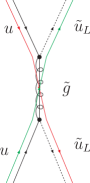
(a) CNS exchange

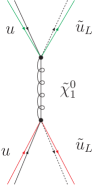
(b) CS exchange

(c) non–rapidity gap event

(d) rapidity–gap event

Figure 1: The two Feynman diagrams show $t-$channel $2\rightarrow 2$ scattering for color non–singlet (CNS) and color singlet (CS) exchange. The colored lines denote the color flow between the incoming quarks and outgoing squarks. The two lower diagrams indicate the color flow of the green (thick line) and red (thin line) color charge in the center of mass system; the circles lie in the rapidity ranges which are filled up by the gluon radiation off the scattered color charges.

The pattern of gluon radiation in these reactions, which may or may not lead to a rapidity gap, can be explained using the picture of an accelerated color charge [12]. Figs. 1(c),(d) sketch the momentum as well as color flow for these reactions in the center–of–mass system (CMS). For a $t-$channel color non–singlet (CNS) exchange process the green color charge of Fig. 1(a) has to scatter from the momentum direction $p_{2}$ to $k_{1}$, i.e. over an angle $\pi-\Theta_{CMS}$, with small $\Theta_{CMS}$ being preferred dynamically. As a result, we expect “bremsstrahlung” gluons to be emitted by the “green” charge over most of the angular, or rapidity, region, as indicated by the large green circle. The “red” charge is also scattered by an angle $\pi-\Theta_{CMS}$. For the dynamically preferred case $\Theta_{CMS}<\pi/2$ we therefore expect the entire rapidity region to be filled with soft gluon radiation; no “gap” arises. This also holds for squared $u-$channel color non–singlet exchange. Here the “green” color flows from $p_{2}$ to $k_{2}$, but $\Theta_{CMS}$ close to $\pi$ is preferred dynamically.

Now consider squared color singlet (CS) $t-$channel contribution, as sketched in Fig. 1(d). In this case the “green” color is accelerated from direction $p_{2}$ to direction $k_{2}$, i.e. it is scattered by $\Theta_{CMS}$, with small $\Theta_{CMS}$ being dynamically preferred. The resulting bremsstrahlung will mainly populate the region indicated by the small green circle. Similarly, bremsstrahlung from the “red” color will mainly populate the region indicated by the small red circle. Note that for $\Theta_{CMS}<\pi/2$, little or no soft bremsstrahlung is expected to occur in the region between the two squarks, leading to the occurrence of a rapidity gap.

It should be noted, however, that according to this argument the gap probability is not exactly zero even in CNS exchange contributions. For example, the squared $t-$channel diagram also contributes at $\Theta_{CMS}\sim\pi$, which, according to the above argument, should lead to a rapidity gap. Conversely, the probability for emission into the gap vanishes only in the limit of vanishing gluon momentum. This implies that emission into the gap is possible, although the corresponding probability is not enhanced by large logarithms. These arguments imply that one will not be able to distinguish between CS and CNS exchange contributions on an event–by–event basis. We do nevertheless expect significant differences in distributions of observables that are sensitive to QCD radiation.

2.2 Simple Monte Carlo Simulations

The discussion of the previous Subsection indicates that the angular distribution of gluons in $qq\rightarrow\tilde{q}_{L}\tilde{q}_{L}g$ events should be very different for CNS and CS exchange contributions. As a first step, we want to verify this expectation using an explicit parton level calculation. Here, as for all our numerical studies, we assume the mSUGRA [17] benchmark scenario SPS1a [18] ($m_{0}=100$ GeV, $m_{1/2}=250$ GeV, $A_{0}=-100$ GeV, $\tan\beta=10\Rightarrow m_{\tilde{q}}=560$ GeV) with conserved $R-$parity. Events are generated using the event generator MadGraph [19], using the pre–defined SPS1a table of sparticle masses and branching ratios. We use the CTEQ5L [20] parameterization of the parton distribution functions; correspondingly the one–loop expression for the strong gauge coupling with five active flavors is taken, where $\Lambda_{\rm{QCD}}=142$ MeV. For simplicity we only consider the case $q=u$. Since the QCD effects we are interested in are flavor blind, it is not necessary to generate the full set of combinations of initial and final flavors [4]. We regulate infrared singularities by requiring the gluon to have a transverse momentum in excess of 20 GeV. This is still soft on the scale of the hard process ($m_{\tilde{q}}\simeq 560$ GeV), i.e. the arguments presented in the previous Subsection should still be valid. We also require the squarks to have pseudorapidity $|\eta|\leq 3.2$.

In the following we plot histograms of the quantity $\Delta$ defined as:

$$\Delta=\frac{\eta_{g}-(\eta_{1}+\eta_{2})/2}{|\eta_{1}-\eta_{2}|/2}\,,$$ (1)

where $\eta_{g}$ is the rapidity of the gluon and $\eta_{1(2)}$ is the rapidity of the first (second) final state squark. Therefore a gluon radiated into the rapidity region spanned by the two squarks ($\eta_{1}<\eta_{g}<\eta_{2}$ for $\eta_{1}<\eta_{2}$ ) gives rise to $\Delta<1$, whereas a gluon outside of this region ($\eta_{g}<\eta_{1},\eta_{2}$ or $\eta_{g}>\eta_{1},\eta_{2}$) leads to $\Delta>1$. Recall that the squarks are kept stable in this Section.

We generated samples of 10,000 events each with pure squared CS and CNS exchange contributions. This is a further simplification, since in reality CS (neutralino) and CNS (gluino) exchange contributions can interfere; we will come back to this point shortly. We do include interference between $t-$ and $u-$channel contributions within each class of events.

Since we wish to look for rapidity gaps, we require the two squarks in the final state to be well separated in rapidity:

$$\Delta\eta=|\eta_{1}-\eta_{2}|\,\geq 3.0\,.$$ (2)

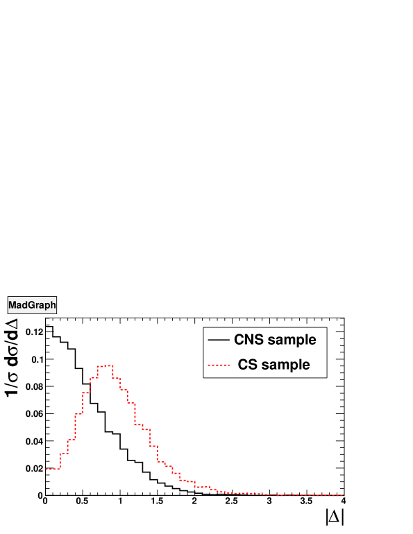
Figure 2: Normalized $\Delta$–distributions of the process $uu\rightarrow\tilde{u}_{L}\tilde{u}_{L}g$ for events generated by MadGraph. Only events passing the cut (2) are included in the distribution and used for the calculation of the integrated cross section $\sigma$. The black (solid) curve denotes the results for the CNS sample (gluino exchange) and the red (dashed) curve denotes the results for the CS sample (neutralino) exchange. Here, as well as in all subsequent numerical results, we use the nominal LHC energy, $\sqrt{s}=14$ TeV.

The resulting normalized $\Delta$ distributions, shown in Fig. 2, confirm our expectation. The CNS distribution has its maximum around $\Delta=0$, i.e. in the middle between the squarks. It decreases approximately linearly with increasing $\Delta$ values as long as $\Delta\raisebox{-3.69899pt}{~{}\shortstack{$<$ \\ [-0.07cm] $\sim$}}~{}1.5$. In contrast, the CS distribution peaks around $\Delta=0.9$, i.e. near the produced squarks, with steep decreases to both sides. In particular, emission at $\Delta=0$ is strongly suppressed by destructive interference between diagrams where the gluon is emitted off the initial or final state. Note also that, while suppressed, the CS distribution does not vanish even at $\Delta=0$, confirming the caveat we made at the end of the previous Subsection.

A parton–level simulation is not sufficient to demonstrate the existence of an experimentally detectable rapidity gap; rather, full hadron–level simulations are needed. We employ the two generators PYTHIA 6.4 [21] and Herwig++ [22]; in PYTHIA 6.4, the old shower model, i.e. the virtuality ordered showering model, is used. These generators can simulate full events, including parton showers, underlying event and hadronization. However, we first want to check that they reproduce the exact radiation pattern shown in Fig. 2. To this end, we generate $uu\rightarrow\tilde{u}_{L}\tilde{u}_{L}$ events with MadGraph. The parton level events are then interfaced via the SUSY Les Houches Accord [23] to the event generators.

This requires that the color flow of each event is specified. We do this following the procedure of Ref. [24], which is also used by MadGraph. Here, all contributions to a single $2\rightarrow 2$ scattering process like $uu\rightarrow\tilde{u}_{L}\tilde{u}_{L}$ are split up according to their different color flows, labeled by $i$:

$${\cal M}=\sum_{i}{\cal M}_{i}\,.$$ (3)

Note that parton shower algorithms generating initial and final state radiation work with probabilities rather than with quantum field theoretical amplitudes. However, simply generating a color flow with probability determined by $\left|{\cal M}_{i}\right|^{2}$ could lead to the wrong total, color–summed probability for generating the given final state: since different ${\cal M}_{i}$ can interfere, $\left|{\cal M}\right|^{2}\neq\sum_{i}\left|{\cal M}_{i}\right|^{2}$. Following Ref. [24], we therefore re–scale the $\left|{\cal M}_{i}\right|^{2}$:

$$\left|{\cal M}_{\rm{full},i}\right|^{2}=\frac{\left|{\cal M}\right|^{2}}{\sum_{i}\left|{\cal M}_{i}\right|^{2}}\left|{\cal M}_{i}\right|^{2}\,.$$ (4)

Note that all $\left|{\cal M}_{\rm{full},i}\right|^{2}$ are positive definite [24]. Moreover, by construction $\sum_{i}\left|{\cal M}_{\rm{full},i}\right|^{2}=\left|{\cal M}\right|^{2}$. We can thus generate events with color flow $i$ with probability determined by $\left|{\cal M}_{\rm{full},i}\right|^{2}$.

Nevertheless this method does not properly include the interference between terms with different color flow, except in the overall normalization. This is considered acceptable, since these terms are suppressed by inverse powers of the number of colors $N_{c}$. We will follow this practice, and drop all terms that are suppressed by inverse powers of $N_{c}$.

To be specific, consider the process $q_{i}q_{j}\rightarrow\tilde{q}_{k}\tilde{q}_{l}$, where $i,j,k,l\in\{1,2,3\}$ are color indices. Strong and electroweak $t-$ and $u-$channel diagrams then generate two color flows. Flow “1” is defined through the color tensor $\delta_{il}\delta_{jk}$, i.e. the color flows from the first quark to the second squark, and from the second quark to the first squark; flow “2” is defined through the tensor $\delta_{ik}\delta_{jl}$, i.e. the color flows from the first quark to the first squark, and from the second quark to the second squark. In the following we drop possible $s-$channel contributions. These have small matrix elements; at the LHC they are further suppressed since they require the existence of an antiquark in the initial state [4]. We then have

$${\cal M}_{1} = {\cal M}_{t,{\rm QCD}}+{\cal M}_{u,{\rm EW}}\,;$$

$${\cal M}_{2} = {\cal M}_{u,{\rm QCD}}+{\cal M}_{t,{\rm EW}}\,.$$ (5)

Here, ${\cal M}_{t,QCD}$ describes $t-$channel gluino exchange, ${\cal M}_{u,{\rm EW}}$ describes the exchange of an electroweak gaugino in the $u-$channel, and so on.

Recall that in Fig. 2 we had considered pure CNS or pure CS exchange. In order to compare these “exact” (leading order) matrix element results with the results of PYTHIA and HERWIG++, we therefore “switch off” either the QCD or the electroweak contributions. To leading order in $1/N_{c}$ there is then a one–to–one correspondence between Feynman diagrams and color flows, i.e. each diagram has a unique color flow, and each color flow only gets contributions from one type of diagram. Moreover, we require at least one gluon to have $p_{T}>20$ GeV. We generated 30,000 events for each simulation, in order to obtain a similar number of events after cuts as in the MadGraph simulation.

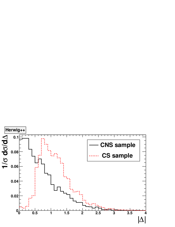
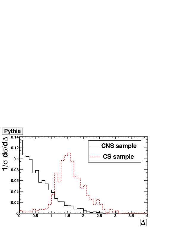
Figure 3: Normalized $\Delta-$distributions for gluon radiation simulated with Herwig++ (top) and PYTHIA 6.4 (bottom). Labeling as in Fig. 2.

In Fig. 3 we show the resulting normalized $\Delta$ distributions for the gluon with the largest $p_{T}$, as predicted by HERWIG++ (top) and PYTHIA 6.4 (bottom). We see that both event generators predict large differences between CNS and CS exchange, in qualitative agreement with the MadGraph prediction of Fig. 2.

However, there are also significant discrepancies between the three predictions. In the CNS case, PYTHIA 6.4 closely reproduces the MadGraph prediction, whereas HERWIG++ generates a distribution that extends to larger values of $\Delta$, leading to a less pronounced peak at $\Delta=0$. In the CS case, PYTHIA 6.4 generates a distribution that peaks at $\Delta\simeq 1.5$, quite far away from the squarks, with very few gluons populating the region $\Delta<0.5$. We should mention here that the “new shower” model of PYTHIA 6.4, which became the default model in the C++ version of PYTHIA [25], failed to predict a gap even in the pure CS exchange case. This is why we only show results based on the “old” showering algorithm; it is based on virtuality ordering, with angular ordering imposed a posteriori. In contrast, HERWIG++ predicts the maximum of the distribution to occur at $\Delta\simeq 0.75$, i.e. between the two squarks, with a very rapid fall–off towards smaller $\Delta$. As a result, the HERWIG++ prediction for $\Delta=0$ also falls below the MadGraph result.

We conclude that both event generators reproduce the gross features of the normalized MadGraph prediction. Since the former typically generate several gluons, we do not actually expect exact agreement with the fixed–order prediction of the latter. The comparison also shows significant differences between PYTHIA 6.4 and HERWIG++. In fact, the differences between PYTHIA and Herwig++ become even larger once we consider the unnormalized distributions. In the pure QCD sample, Herwig++ predicts about 35% more events with $\delta\eta\geq 3.0$ to contain at least one gluon with $p_{T}\geq 20$ GeV. In the pure EW sample, this difference between the two generators even amounts to a factor of seven, with Herwig++ again predicting more gluon radiation. At the present time these differences should be interpreted as systematic uncertainties of the predictions. We will therefore continue to show predictions from both generators. In Sec. 4 we will suggest how this uncertainty might be reduced using real data.

2.3 Interference between Color Singlet and Color Non–Singlet Exchange

Before turning to fully realistic simulations, we want to study the effects of interference of CS (neutralino) and CNS (gluino) exchange contributions, which we have ignored so far. In fact, at least as far as the total squark production cross section is concerned, the biggest effect of electroweak gaugino exchange is due to interference with the dominant QCD diagrams [4]. For our benchmark point SPS1a, this increases the total cross section for the production of $SU(2)$ doublet, “$L-$type” squarks by about 16%.

To test the effect of the electroweak CS exchange contribution on the $\Delta$ distribution, we generated 100,000 $uu\rightarrow\tilde{u}_{L}\tilde{u}_{L}g$ events with either pure QCD or QCD$+$EW contributions, again requiring $p_{T}(g)>20$ GeV.

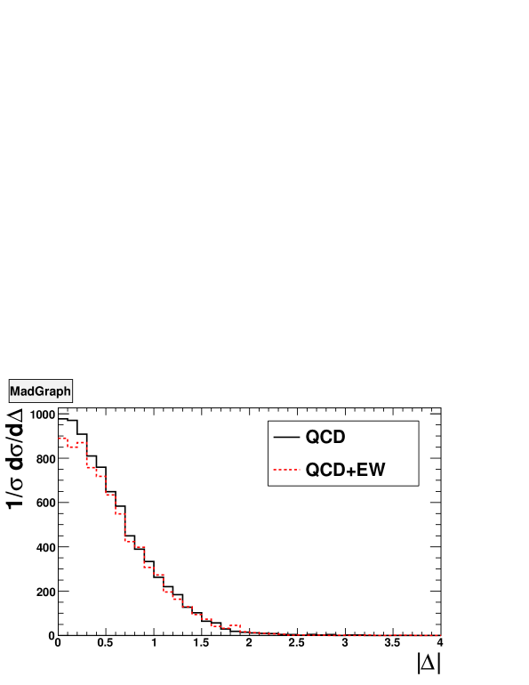
Figure 4: $\Delta$–distributions for gluon radiation simulated with MadGraph. The black (solid) curve denotes the results for the CNS sample (pure QCD exchange particles) and the red (dashed) curve denotes the results for the CNS+CS sample (QCD and EW exchange particles). One has 7962 events after the cut (2) in the pure QCD sample and 7506 events in the mixed QCD+EW sample.

The resulting $\Delta$ distributions are shown in Fig. 4. We are showing unnormalized distributions, because it makes the difference between the two samples more visible and shows the feature of an efficiency reduction.

The latter is illustrated by the fact that the total number of events with two squarks having a rapidity–distance larger than three is 7962 for the QCD sample and 7506 for the QCD+EW sample, so including EW contributions reduces the efficiency of passing the cut of Eq.(2) by $(6.1\pm 1.7)\%$ (statistical error only). This can be explained as follows. Requiring a large $\Delta\eta$ between the two squarks singles out events where the CMS scattering angle $\theta$ is close to either 0 or $\pi$, and with sizable squark CMS velocities $\beta$. The latter condition implies that the $t-$ and $u-$channel propagators depend strongly on $\theta$:

$$\hat{t}-M^{2}_{\tilde{V}}=m^{2}_{\tilde{q}}-\frac{\hat{s}}{2}(1-\beta\cos\theta)-M^{2}_{\widetilde{V}}\,,$$ (6)

where $M_{\tilde{V}}$ is the mass of the exchanged gaugino and $\hat{s},\,\hat{t}$ and $\hat{u}$ are the partonic Mandelstam variables; the expression for $u-$channel propagators can be obtained by the replacement $\cos\theta\rightarrow-\cos\theta$. These propagators prefer large $\beta|\cos\theta|$; however, $t-$ and $u-$channel propagators prefer different signs of $\cos\theta$. Thus a large value of $\Delta\eta$ suppresses the relative importance of the interference of $t-$ and $u-$channel diagrams. We showed in Ref. [4] that the dominant electroweak contributions are precisely due to such interference terms. Moreover, in pure QCD $t-$ and $u-$channel diagrams interfere destructively, which makes the peaks at large $|\cos\theta|$ even more pronounced. Therefore the cut of Eq.(2) reduces the importance of the electroweak contributions.

For $\Delta\leq 0.2$, the difference between the pure QCD and QCD+EW predictions amounts to $\sim 10\%$, larger than the integrated difference of 6% discussed above. Evidently including EW contributions slightly decreases the probability to emit a gluon at small $\Delta$. This can be understood from Eqs.(2.2): ${\cal M}_{1}$, where the color flow will lead to a gap if $\theta\simeq\pi$, receives an electroweak $u-$channel contribution which is in fact peaked at $\theta=\pi$, where the pure QCD contribution is minimal; analogous statements hold for ${\cal M}_{2}$.

The size of the effect seen in Fig. 4 is smaller than one would expect from our observation [4] that EW contributions increase the total cross section for $\tilde{u}_{L}\tilde{u}_{L}$ production by about 16%. There are two reasons for this. First, we argued above that the cut of Eq.(2) reduces the relative size of these interference terms. Secondly, in Fig. 4 we are studying the $2\rightarrow 3$ process $uu\rightarrow\tilde{u}_{L}\tilde{u}_{L}g$. Here including the EW contribution increases the total cross section (with $p_{T}(g)>20$ GeV, but without cut on the squark rapidities) by only 9%. This last observation indicates that Fig. 4 understates the importance of EW contributions: in addition to changing the shape of the $\Delta$ distribution of emitted hard gluons, they also reduce the probability of emitting a hard gluon anywhere in phase space. The importance of this second effect can best be investigated with the help of event generator programs, which produce $\tilde{q}\tilde{q}+n\,g$ events with (approximately) correct relative weight for any $n=0,1,2,\dots$. This is the topic of the next Section.

3 Full Event Simulation

We now turn to full event simulation, including squark decays, hadronization, jet reconstruction and the “underlying event”, however without simulating the detector. To be specific, we consider rapidity–gap events for squark pair production at the LHC, where electroweak (EW) contributions at tree level are included. The production of the first two generations of squarks via $t-$ and $u-$channel diagrams is taken into account. $s-$channel contributions are neglected, since they are quite small [4], and are not expected to lead to rapidity–gap events. Quark mass effects, the mixing between $SU(2)$ doublet and singlet squarks and flavor mixing effects are neglected. The mass spectrum and branching ratios of the sparticles are obtained from SPheno [26]. Analytical expressions for the squared and averaged matrix elements are given in Ref. [4]. We implemented the relevant matrix elements for QCD and as well for EW contributions in a simple parton–level simulation. Jets are reconstructed via the $k_{T}$ clustering algorithm of FastJet [27]. Events are analyzed using the program package root [28].

We saw in Subsec. 2.2 that the angular distributions of the hardest gluons in PYTHIA 6.4 (with the “old” shower algorithm) and Herwig++ roughly agrees with an “exact” (leading order) MadGraph calculation. We therefore continue to use these two generators, hoping that the difference between their predictions can be used as a measure of the current theoretical uncertainty.

Our goal is to find evidence for the different color flows in CS (EW) and CNS (pure QCD) exchange contributions. In Ref. [4] we have shown that production of two $SU(2)$ doublet squarks receives the largest EW contributions, partly because the $SU(2)$ gauge coupling is larger than the $U(1)_{Y}$ gauge coupling. Moreover, most relevant matrix elements are proportional to the mass of the exchanged gaugino, and in mSUGRA winos are about two times heavier than the bino. For example, in SPS1a, the cross section for production of two $SU(2)$ doublet squarks is enhanced by $13\%$ by the EW contributions. If at least one $SU(2)$ singlet squark is in the final state, EW contributions are much smaller, leading to an increase of the total squark pair production cross section of only $4$%. In order to enhance the importance of the EW contributions, and hence the rapidity gap signal, we thus look for cuts that single out the contribution from the pair production of $SU(2)$ doublet squarks.

This is possible at least for $m_{\tilde{g}}\raisebox{-3.69899pt}{~{}\shortstack{$>$ \\ [-0.07cm] $\sim$}}~{}m_{\tilde{q}}>|M_{2}|,|M_{1}|$, which is true for the SPS1a benchmark point we are considering. In this case $SU(2)$ singlet squarks prefer to decay into the neutralino with the largest bino component [29], which is usually the $\tilde{\chi}_{1}^{0}$ in mSUGRA. In contrast, $SU(2)$ doublet squarks prefer to decay into charginos and neutralinos dominated by wino components [29], which are typically the $\tilde{\chi}_{2}^{0}$ and $\tilde{\chi}_{1}^{\pm}$ in mSUGRA. Since $\tilde{\chi}_{1}^{0}$ is stable while $\tilde{\chi}_{2}^{0}$ and $\tilde{\chi}_{1}^{\pm}$ can decay leptonically, the relative contribution of doublet squarks can be enhanced experimentally by requiring the presence of energetic, isolated charged leptons, in addition to $\geq 2$ jets and missing transverse momentum [30]. By requiring the presence of two leptons with equal charges we single out events where both squarks decay semi–leptonically; in contrast, events with two oppositely charged leptons could come from $\tilde{q}_{R}\tilde{q}_{L}$ production followed by $\tilde{q}_{L}\rightarrow q\tilde{\chi}_{2}^{0}\rightarrow q\ell^{+}\ell^{-}\tilde{\chi}_{1}^{0}$ decays ($\ell=e,\,\mu,\,\tau$). Note that we do not veto the presence of additional charged leptons, i.e. we also accept events with three or four charged leptons.

In SPS1a, $SU(2)$ doublet squarks $\tilde{q}_{L}$ almost always decay into either $\tilde{\chi}_{1}^{\pm}q^{\prime}$ or into $\tilde{\chi}_{2}^{0}q$, with relative frequency of approximately $2:1$. The electroweak gauginos $\tilde{\chi}_{2}^{0}$ and $\tilde{\chi}_{1}^{\pm}$ in turn almost always decay leptonically. Our requirement of two like–sign charged leptons therefore accepts nearly all $\tilde{u}_{L}\tilde{u}_{L}$ and $\tilde{d}_{L}\tilde{d}_{L}$ pair events, as well as more than half of $\tilde{u}_{L}\tilde{d}_{L}$ events (rejecting only events where both $\tilde{u}_{L}$ and $\tilde{d}_{L}$ decay into a chargino). Most of the charged leptons produced in $\tilde{\chi}_{2}^{0}$ and $\tilde{\chi}_{1}^{\pm}$ decays are $\tau$ leptons. For the sake of simplicity, we assume that the $\tau$ detection efficiency is 100$\%$. The final state from the production of two $SU(2)$ doublet squarks thus typically contains two or more $\tau$ leptons, $\geq 2$ jets and missing $E_{T}$.

Altogether we therefore impose the following cuts. We require that the two highest transverse momentum jets satisfy

$$E_{T}(j_{i})\geq 100\,{\rm GeV}\,;\quad\left|\eta(j_{i})\right|\leq 5.0\quad(i=1,2).$$ (7)

We further suppress SM backgrounds by requiring a large amount of missing transverse energy,

$$E_{T}/\hskip 12.80373pt\geq 100\,{\rm GeV}.$$ (8)

Squark pair events containing at least one $SU(2)$ singlet squark are suppressed by requiring the existence of two like–sign charged leptons, with

$$p_{T}(\ell_{i})\geq 5\,{\rm GeV}\,;\quad\left|\eta(\ell_{i})\right|\leq 2.4\quad(i=1,2).$$ (9)

In order to be able to define a meaningful rapidity gap, the two leading jets should be well separated in rapidity:

$$\Delta\eta\equiv\left|\eta(j_{1})-\eta(j_{2})\right|\geq 3.0\,.$$ (10)

We have to take into account that the two jets have finite radii. The gap region is therefore defined as

$$\rm{min}[\eta(j_{1}),\eta(j_{2})]+0.7\leq\eta\leq\rm{max}[\eta(j_{1}),\eta(j_{2})]-0.7\,.$$ (11)

One can expect that most of the particles produced during hadronization are within the cone of $0.7$ of the corresponding jets [31].

Since we want to avoid “event pile–up”, i.e. multiple $pp$ interactions during the same bunch crossing, we assume an integrated luminosity of 40 fb^-1 at $\sqrt{s}=14$ TeV. Using LO cross sections [4], this corresponds to about $484,000$ squark pair events for pure QCD, about $121,000$ of which contain two $SU(2)$ doublet squarks; these numbers increase to $502,000$ (all squark pairs) and $140,000$ (only $SU(2)$ doublets) events once electroweak contributions are included.

In our simulation we generated squark pair events, with sample sizes equal to the expected numbers of events given above. After applying all cuts, in the Herwig++ simulation, 3574 and 4032 events remain in the QCD and QCD+EW samples, respectively. In the PYTHIA 6.4 simulation, 3271 QCD and 3723 QCD+EW events are retained. The overall efficiency of our cuts relative to the entire squark pair sample is therefore less than 1%. Of course, this is partly desired. Focusing on the production of two $SU(2)$ doublets reduces the number of events by a factor of about four. Moreover, we saw above that requiring two like–sign leptons removes nearly half of all $\tilde{d}_{L}\tilde{u}_{L}$; this is a pity, since in this channel the EW contributions are relatively most important [4]. This reduces the event samples by another factor of about 1.3.

Since most “primary” jets from squark decay are quite central, the cut of Eq.(10) reduces the event samples by another factor of about 15. We note that the efficiency of this cut is higher than that of the analogous cut of Eq.(2) applied to the squarks: since squark decays release a large amount of energy, the jets resulting from these decays can be further apart in rapidity than the decaying squarks, if the quarks are emitted in a direction close to the flight direction of their squark parents. Since the cut of Eq.(10) favors such configurations, in most of the accepted events, squark decay will not lead to an additional acceleration of the color charge over a large angle. The discussion of the previous Subsection regarding the angular region covered by QCD radiation should therefore remain qualitatively correct. Finally, almost half of the remaining events are removed by the kinematical cuts of Eqs.(7), (8) and (9). We note that the total cut efficiency for events containing two $SU(2)$ doublet squarks is nearly the same for the pure QCD and QCD+EW samples after summing over all channels.

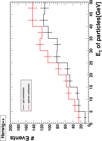
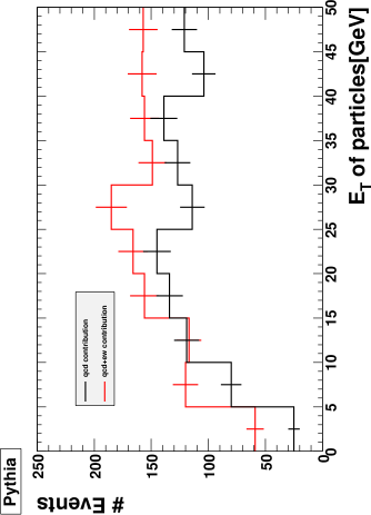
Figure 5: Transverse energy in the rapidity–gap region (11) as predicted by full event simulations of squark pair production using HERWIG++ (top) and PYTHIA 6.4 (bottom). Black histograms show pure QCD results, while the red (gray) histograms include electroweak contributions. The errors are statistical only.

Our first attempt to isolate “rapidity gap events” uses a completely inclusive quantity. We define $E_{T,{\rm particles}}^{\rm{gap}}$ as the total transverse energy deposited in the gap region defined in Eq.(11); this is computed from all photons and hadrons in the event (after hadronization and decay of unstable hadrons), but does not include the leptons produced in $\tilde{\chi}^{0}$ and $\tilde{\chi}^{\pm}$ decays. The distribution of $E_{T,{\rm particles}}^{\rm{gap}}$ is shown in Fig. 5 for Herwig++ (top) and PYTHIA 6.4 (bottom). In this and all following figures, black and red histograms denote pure QCD and QCD+EW predictions, respectively. We also show the statistical error for each bin.

We note that including EW contributions increases the number of events, although in most bins this effect is statistically not very significant. However, in the first bin, where the total $E_{T}$ is less than 5 GeV, the inclusion of these CS exchange contributions increases the number of events by a factor of $2.8\pm 1.1$ and $2.36\pm 0.56$ in the Herwig++ and PYTHIA 6.4 simulations, respectively. This indicates that CS exchange does lead to “gap” events where little or no energy is deposited between the two hard jets.

However, only 0.6% (1.6%) of all events passing our cuts in Herwig++ (PYTHIA 6.4) are true gap events in this sense. Evidently PYTHIA predicts many more such gap events. This may partly be due to the differences in showering off CS exchange events seen in Fig. 3. However, PYTHIA also predicts many more gap events in a pure QCD (CNS exchange) simulation. We remind the reader that PYTHIA predicted significantly fewer events to contain a hard gluon even in a pure SUSY QCD sample. Moreover, the two event generators not only use different parton shower algorithms; their modeling of hadronization, and of the underlying event, also differs. Overall, the difference between the two generators is as large as the effect from the CS events: PYTHIA 6.4 without CS exchange contributions predicts almost exactly the same number of events in the first bin as Herwig++ with CS exchange. PYTHIA 6.4 also predicts a $E_{T,{\rm particles}}^{\rm{gap}}$ distribution which is quite flat beyond 20 GeV, whereas the distribution predicted by Herwig++ flattens out only at about 40 GeV. One might thus be able to use the higher bins, where the effect of the CS exchange contributions is not very sizable, to decide which generator describes the data better, or to tune the Monte Carlo generators to the data. This should reduce the difference between the two predictions.

The results of Fig. 5 only include contributions from squark pair production. Non–supersymmetric backgrounds are negligible after our basic cuts of Eqs.(7)–(10). However, other supersymmetric final states may contribute; in the present context they have to be considered as background. Owing to the large cross section, events containing at least one gluino in the final state are of particular concern.

In order to check this, we generated all hard SUSY $2\rightarrow 2$ processes with at least one gluino in the final state using PYTHIA. These processes add up to a cross section of about 24 pb for SPS1a, which exceeds the squark pair production cross section by a factor of two. With only the basic cuts of Eqs.(7)–(10), these additional contributions more than double the entries of the first $E_{T}$ bin in Fig. 5, compared to the result for CNS squark pair production. This would reduce the significance noticeably. However, gluino events practically always contain at least one additional hard jet from $\tilde{g}\rightarrow\bar{q}+\tilde{q},\ q+\tilde{q}^{*}$ decays. This SUSY background can thus be suppressed efficiently, with negligible loss of signal, by vetoing the presence of a third energetic jet. In the following we therefore continue to focus on squark pair events.

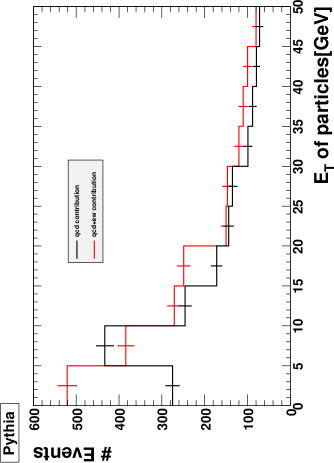
Figure 6: Same as Fig. 5, bottom frame (PYTHIA 6.4 prediction), except that the underlying event has been switched off.

One reason for the small number of true gap events, and the correspondingly large statistical error, is the energy deposition of the “underlying event”, which describes the beam remnants. These “spectator partons” do not participate in the primary partonic squark pair production reaction, but may interact via semi–hard QCD reactions [32]. The underlying event can thus deposit a significant amount of transverse momentum, with little or no phase space correlation with the primary jets. The importance of this component of the total $E_{T}$ flow is illustrated in Fig. 6, which shows the PYTHIA 6.4 prediction for the total $E_{T,{\rm particles}}^{\rm{gap}}$ distribution with the underlying event switched off. Clearly the first few bins now contain many more events than in Fig. 5. For example, we now have 521 (278) entries in the first $5$ GeV bin for QCD+EW (QCD) simulation, as compared to 59 (25) in Fig. 5. Recall that including EW contributions increased the PYTHIA 6.4 event sample after cuts by only about 450 events; evidently about 50% of these additional events would be true gap events, if the underlying event were absent. The underlying event in PYTHIA 6.4 thus leads to a gap “survival probability” [10] of $\sim 10\%$ at the LHC.

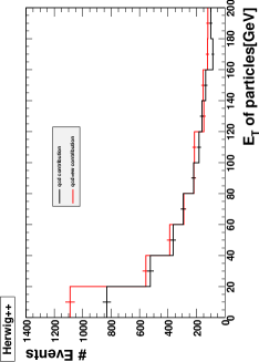
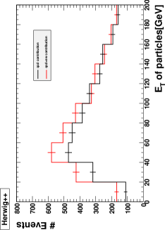
Figure 7: Same as Fig. 5, top frame (Herwig++ prediction), except that the $x-$axis has been extended to 200 GeV; moreover, in the left frame the underlying event has been switched off.

The left frame of Fig. 7 shows analogous results for the Herwig++ simulations, where we have extended the $x-$axis to 200 GeV. In this case, only about 50% of the additional events due to EW interactions appear in the first bin, even though the bin width has been increased to 20 GeV; we again observe a smaller effect due to CS exchange than in the PYTHIA simulation. Note that also the pure QCD prediction now peaks in the first (wide) bin. In Herwig++ the underlying event typically deposits about 45 GeV of transverse energy in the gap. Switching this effect on thus leads to distributions with broad peaks around 50 GeV, as shown in the right frame of Fig. 7.

Of course, the $E_{T}$ deposited by the underlying event differs from event to event. Therefore some true gap events do remain even if the underlying event has been switched on, as we saw above. In fact, the effect of the underlying event is somewhat larger in the pure QCD simulations than in the QCD+EW case. In the Herwig++ simulation of Fig. 7, the underlying event reduces the number of events in the first bin for the pure QCD (QCD+EW) simulation by about a factor of eight (six). Figs. 5 and 6 show a similar effect for PYTHIA 6.4: the underlying event reduces the number of events in the first (5 GeV wide) bin by a factor of about ten (eight) for the pure QCD (QCD+EW) case. This is not implausible, since the beam remnants are color connected to the partons participating in squark pair production, leading to some correlation between the “hard” and “underlying” parts of the total event.

The significance of the enhanced rapidity gap signal due to EW effects depends on how exactly the comparison is done. Let us focus on Herwig++ predictions for definiteness; PYTHIA predicts somewhat larger significances. Simply looking at the first bin of Fig. 5 gives a statistical significance of about 2.5$\sigma$ given the current MC statistics. However, in an experiment one would compare the actual event number with a prediction of pure QCD. Assuming this prediction indeed remained at 9 events with negligible MC error, and the experiment indeed counted 25 events, the statistical significance would be $16/\sqrt{9}=5.3\sigma$! On the other hand, the absolute normalization of the curves in Figs. 5 and 7 cannot really be trusted, since they rely on LO cross sections. If we want to analyze the change of the shape of the distribution, the larger $E_{T}$ range depicted in Fig. 7 is more appropriate. According to the right frame of that figure, pure QCD and QCD+EW predictions agree to 2% when all bins with $E_{T}\geq 100$ GeV are summed. The sum up to 100 GeV then differs by 5.3$\sigma$ according to current MC statistics; this could become 8 standard deviations with infinite MC statistics, assuming the central values remain the same.

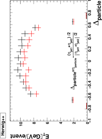
Figure 8: The average amount of deposited transverse energy per bin as a function of $\Delta$ as predicted by Herwig++. The black (red or grey) points denote the results for the pure QCD (QCD+EW) sample. The vertical error bars indicate the statistical uncertainty, while the horizontal bars show the bins.

We also studied the average $E_{T}$ flow as a function of the scaled rapidity variable $\Delta$, defined analogously to Eq.(1):

$$\Delta=\frac{\eta-\left[\eta(j_{1})+\eta(j_{2})\right]/2}{\left|\eta(j_{1})-\eta(j_{2})\right|/2}\,.$$ (12)

The $E_{T}$ flow in the gap region as predicted by Herwig++ is shown in Fig. 8. Recall that the rapidity gap region as defined in Eq.(11) is somewhat smaller than the region $|\Delta|<1$; this explains the sharp drop of the average deposited $E_{T}$ for $|\Delta|>0.6$. We see that including EW, CS exchange contributions reduces the average deposited $E_{T}$ by about 8%, or 8.5 GeV per unit of $\Delta$, around $\Delta=0$. The error bars in Fig. 8 show that this effect is statistically quite significant. However, given the large modeling uncertainty, and the sizable energy measurement errors, the size of the effect is presumably too low to be physically significant.

Predicting the total transverse energy flow is difficult, since this observable is strongly affected by semi– and non–perturbative effects. We could try to reduce the importance of these effects by focusing on charged particles whose $p_{T}$ exceeds a few GeV [11]. Instead we go one step further and discuss the occurrence of relatively soft “minijets” in the “gap region” defined in Eq.(11).

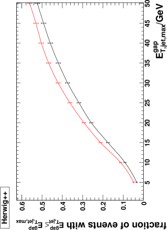
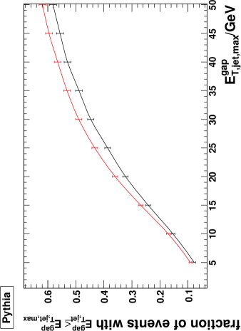
Figure 9: Fraction of squark pair events passing a minijet veto in the rapidity–gap region (11), as predicted using full event simulations using Herwig++ (top) and PYTHIA 6.4 (bottom). The black curve is for the pure QCD sample, and the red (gray) curve for the QCD+EW sample.

Fig. 9 shows the fraction of events where the energy $E_{T,\rm{jet}}^{\rm{gap}}$ of the most energetic jet in the gap region (11) is less than the value $E_{T,\rm{jet,max}}^{\rm{gap}}$ displayed on the $x-$axis. Since Fig. 9 shows event fractions, all curves asymptotically approach 1 at large $E_{T,\rm{jet,max}}^{\rm{gap}}$. We assume that jets with transverse energy above $E_{T,{\rm thresh}}=5$ GeV can be reconstructed. If the true threshold is higher, the curves should simply be replaced by constants for $E_{T,\rm{jet,max}}^{\rm{gap}}\leq E_{T,{\rm thresh}}$. We expect that the underlying event by itself generates few, if any, reconstructable jets. The results here are nevertheless still not quite immune to non–perturbative effects, since reconstructed jets may also contain a few particles stemming from the underlying event. Note also that a jet whose axis lies in the gap region might contain (mostly quite soft) particles that lie outside of this region. Conversely, even though we use a cluster algorithm, where by definition each particle belongs to some jet, some particles in the gap region might be assigned to a jet whose axis lies outside this region.

We see that PYTHIA 6.4 (lower frame) predicts more events without jet in the gap region than Herwig++ (upper frame). This is consistent with Fig. 5, where PYTHIA also predicted more events with little or no energy deposited in the gap region. It also conforms with our observation at the end of Subsec. 2.2 that PYTHIA tends to generate fewer hard gluons than Herwig++ does. In fact, for $E_{T,{\rm jet,max}}^{\rm gap}=20$ GeV, which corresponds to the cut $p_{T}(g)>20$ GeV employed in Subsec. 2.2, we again find a ratio of about 1.3 between the PYTHIA and Herwig++ predictions for the pure SUSY QCD case.

Moreover, both PYTHIA 6.4 and Herwig++ predict a significant increase of the fraction of events without jet in the gap region once EW, CS exchange contributions are included; the effect is statistically most significant for $E_{T,\rm{jet,max}}^{\rm{gap}}\sim 20$ to 40 GeV. Here both generators predict an increase of the fraction of events without (sufficiently hard) jet in the gap by about 0.05. Taking a threshold energy of 30 GeV as an example, Herwig++ predicts about 1,570 out of the total of 4,032 events without jet in the gap once EW effects are included. This should allow to measure the fraction of events without jet in the gap to an accuracy of about 0.01; a shift of the jet–in–the gap fraction by 0.05 thus corresponds to a change by about five standard deviations (statistical error only).

Unfortunately a pure SUSY QCD PYTHIA simulation leads to a fraction of events without jet of 0.45 for the same threshold energy, which is higher than the Herwig++ prediction including EW contributions. Clearly these large discrepancies between the two MC generators have to be resolved before reliable conclusions about the color flow in squark pair events can be drawn.

4 Tuning MC Generators with SM QCD

We saw in the last Section that the systematic differences between PYTHIA and Herwig++ are larger than the physical differences between the QCD and QCD+EW data samples. In this Section, we demonstrate that PYTHIA and Herwig++ make similarly different predictions for standard QCD di–jet events. These pure QCD events can thus be used to tune the Monte Carlo generators. Here “tuning” refers to both the setting of parameters (shower scales etc.), and to details of the algorithms used to describe parton showers and the underlying event.

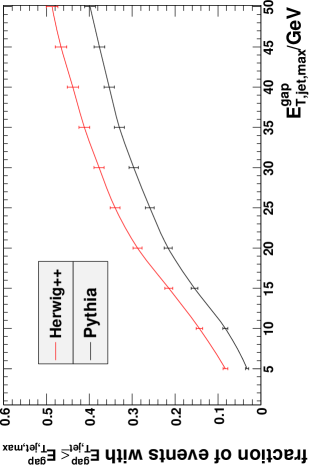
Figure 10: Fraction of events without hard jet in the rapidity–gap region for the pure QCD $2\rightarrow 2$ processes as function of the jet energy threshold. The effects of the underlying event, parton shower and hadronization are included. The black (red) curve denotes the results for PYTHIA (Herwig++).

To illustrate this, we generated standard QCD di–jet events, where we require the transverse momentum of the jets to exceed 500 GeV, so that the kinematics and the relevant Bjorken$-x$ values are comparable to the squark pair events discussed in the two previous Sections. We include all standard QCD $2\rightarrow 2$ processes, i.e. we do not demand that the final state only consists of quarks. The color structure may therefore be different than in SUSY QCD squark pair events. However, the large transverse momentum, as well as the required large rapidity gap, require quite large Bjorken$-x$ values. This enhances the contribution from $qq\rightarrow qq$ scattering, which has exactly the same color structure as the $qq\rightarrow\tilde{q}\tilde{q}$ events in SUSY QCD.

The results are shown in Fig. 10, where we again plot the fraction of events without hard jet in the gap region, as function of the threshold energy. We see that PYTHIA again predicts less radiation, i.e. more events without hard jet in the gap. For example, for a threshold energy of 20 GeV, we find the by now familiar ratio of about 1.3 between the predictions of Herwig++ and PYTHIA. This difference is statistically highly significant. Quite likely neither of the two predictions presented here will turn out to be exactly correct. However, given their many successes in describing quite intricate features of hadronic events, we are confident that soon after real data for this jet–in–the–gap fraction become available, updated versions of both PYTHIA and Herwig++ will be produced that are able to reproduce these data. It seems likely that these advanced versions will then also make very similar predictions for observables that are sensitive to the color flow in squark pair events.

We conclude this Section with two remarks. First, the fraction of events without a hard jet in the gap is significantly smaller in Fig. 10 than for the case of squark pair production shown in Fig. 9. This is mostly due to the remaining contribution containing at least one gluon in the hard $2\rightarrow 2$ process, in either the initial or final state. Note that gluon emission off gluons is enhanced by a color factor of 9/4 relative to gluon emission off quarks. The presence of a gluon in the hard processes thus increases the probability of emitting a rather energetic gluon in the parton shower.

Secondly, the pure QCD prediction for the jet–in–the–gap cross section at the LHC has recently been calculated [33]. Their final result agrees quite well with predictions of Herwig++; no comparison with PYTHIA is provided. However, this agreement is partly accidental. On the one hand, the theoretical calculation is asymptotic in the sense that energy conservation is not enforced. On the other hand, it includes true quantum effects which cannot be fully included in a conventional MC generator that works with probabilities rather than amplitudes. We conclude that, while such comparisons between MC generators and advanced parton level calculations are certainly useful and important, they cannot replace a comparison with real data.

5 Summary and Conclusions

In this paper we analyzed rapidity gap events in squark pair production, where QCD as well as electroweak (EW) contributions were taken into account. The different flow of color charges in the two cases led us to expect that events with EW gaugino exchange should have a higher probability to show a rapidity gap between the produced squarks, where little or no energy is deposited, since radiation into the gap region should be suppressed. An explicit fixed–order calculation of the $2\rightarrow 3$ process $uu\rightarrow\tilde{u}_{L}\tilde{u}_{L}g$ using MadGraph confirmed this expectation: color–singlet exchange leads to a very different rapidity distribution of the emitted gluon than color–octet exchange.

We also compared this fixed–order calculation to the distribution of the hardest gluon produced by the event generators PYTHIA 6.4 and Herwig++. We confirmed that both generators predict rapidity distributions of hard QCD radiation which are sensitive to the color structure of the event. In the case of color non–singlet exchange we found satisfactory agreement of the normalized distributions between both MC generators and MadGraph. However, the normalized distributions in the case of pure color–singlet exchange are noticeably different between PYTHIA, Herwig++ and MadGraph. Moreover, the MC generators predict quite different probabilities for emitting a gluon with transverse momentum above our cut–off of 20 GeV.

We next included interference between QCD and EW contributions. We showed that the EW $t-$channel diagrams have the same color flow (to leading order in the number of colors) as QCD $u-$channel diagrams, and vice versa. This allows to properly include interference between QCD and EW contributions, which greatly increases the importance of the latter; note that MC generators require a unique color flow be assigned to each event.

In Sec. 3 we performed a full simulation, including the underlying event, the full shower algorithm, squark decay, and the hadronization of all partons. The mSUGRA point SPS1a was employed as a benchmark scenario. We focused on events containing two charged leptons ($e,\,\mu$ or $\tau$) with equal charge in addition to at least two jets; this enhances the contribution from $SU(2)$ doublet squarks, where EW contributions are much more important than for the production of $SU(2)$ singlets.

We found two observables yielding distinct results between pure SUSY QCD simulations and those including EW contributions: the transverse energy of all particles in the “rapidity gap” region between the jets resulting from squark decay, and the fraction of events not containing an additional jet in the gap region with $E_{T}$ above a certain threshold. In the case of the total transverse energy in the gap, we found the most distinct difference between the QCD and QCD+EW predictions in the very first bin, i.e. for the lowest $E_{T}$ values. Not surprisingly, this difference is smeared out considerably when the underlying event is included. The second observable, the jet–in–the–gap cross section, is less sensitive to non– or semi–perturbative effects. Here we found statistically significant differences between the QCD+EW and QCD predictions for a range jet thresholds up to 50 GeV.

Unfortunately, for both observables the systematic difference between PYTHIA and Herwig++ currently make it impossible to make clear–cut predictions. In particular, PYTHIA’s pure QCD prediction is usually comparable to, or even larger than, the QCD+EW prediction of Herwig++. In Sec. 4 we showed that a similar difference between the predictions of the two generators also exists for the jet–in–the–gap cross section in standard QCD. This indicates that such standard QCD events can be used during the earliest phases of LHC running to improve the event generators, hopefully to the extent that the difference between their predictions becomes significantly smaller than the effect from the EW contributions.

We also noted that Herwig++ seems to reproduce sophisticated perturbative QCD calculations of the SM jet–in–the–gap cross section fairly well. If we conservatively assume that the Herwig++ predictions, which lie below those of PYTHIA, are correct also for the SUSY case, the assumed integrated luminosity of 40 fb^-1 will suffice to show evidence for color singlet exchange contributions from the total $E_{T}$ distribution in the gap at the level of about 5 to 8 standard deviations; see the discussion of Figs. 5 and 7. Similarly, for a threshold energy of 30 GeV for the jet in the gap, the fraction of events without a jet in the gap changes by about five standard deviations when EW effects are included, see Fig. 9.

Our analyses were based on standard QCD and EW perturbation theory, augmented by the bells and whistles of the MC generators; it resembles the work of ref.[8] for standard jet production. In particular, we did not include hard QCD color singlet exchange contributions. In standard QCD this becomes possible once several gluons are exchanged. In ref.[9] a (non–asymptotic) version of such “BFKL dynamics” [34] (aka perturbative Pomeron exchange) has been shown to be able to reproduce early Tevatron data [14] on rapidity gaps between jets. In the case at hand one would have to consider exchange of a “perturbative Pomeronino”, which includes simultaneous gluon and gluino exchange in the $t-$ or $u-$channel. We are not aware of any study of this kind of contribution.

Finally, we remind the reader that much larger EW effects are possible if the ratio of electroweak to strong gaugino masses is increased beyond the ratio of approximately 1:3 assumed in mSUGRA. We thus conclude that experimental studies of the color flow in squark pair events, of the kind sketched in this paper, are well worth the effort once the existence of squarks has been firmly established.

Acknowledgments

This work was partially supported by the Helmholtz-Alliance “Physics at the Terascale”. SB wants to thank the “Universitätsgesellschaft Bonn – Freunde, Förderer, Alumni e.V.” and the “Bonn-Cologne Graduate School of Physics and Astronomy” for financial support. JSK wants to thank the Helmholtz-Alliance for financial support and the University of Bonn and the Bethe Center for hospitality during numerous vists. HD would like to thank the Aspen Center for Physics for hospitality, where part of this work was completed.

References

- [1] For introductions to supersymmetry, see e.g. M. Drees, R.M. Godbole and P. Roy, Theory and Phenomenology of Sparticles, World Scientific Publishing Company (2004); H. Baer and X. Tata, Weak Scale Supersymmetry: From Superfields to Scattering Events, Cambridge, UK: Univ. Pr. (2006).
- [2] P.R. Harrison and C.H. Llewellyn Smith, Nucl. Phys. B213, 223 (1983); Erratum ibid. B223, 542 (1983); S. Dawson, E. Eichten and C. Quigg, Phys. Rev. D31, 1581 (1985); H. Baer and X. Tata, Phys. Lett. B160, 159 (1985).
- [3] G. Bozzi, B. Fuks, B. Herrmann and M. Klasen, Nucl. Phys. B787, 1 (2007) [arXiv:0704.1826 [hep-ph]].
- [4] S. Bornhauser, M. Drees, H. K. Dreiner and J. S. Kim, Phys. Rev. D 76 (2007) 095020 [arXiv:0709.2544 [hep-ph]].
- [5] W. Hollik, M. Kollar and M.K. Trenkel, JHEP 0802 (2008) 018 [arXiv:0712.0287 [hep-ph]]; W. Hollik and E. Mirabella, JHEP 0812 (2008) 087 [arXiv:0806.1433 [hep-ph]].
- [6] J. D. Bjorken, S. J. Brodsky and H. J. Lu, Phys. Lett. B 286 (1992) 153.
- [7] H1 Collab., T. Ahmed et al., Nucl. Phys. B 429 (1994) 477; L. Lonnblad, Z. Phys. C 65 (1995) 285; ZEUS Collab., M. Derrick et al., Phys. Lett. B 369 (1996) 55, hep–ex/9510012; A. Edin, G. Ingelman and J. Rathsman, Z. Phys. C 75 (1997) 57, hep–ph/9605281. M. Wusthoff, Phys. Rev. D 56 (1997) 4311, hep–ph/9702201.
- [8] H. Chehime, M. B. Gay Ducati, A. Duff, F. Halzen, A. A. Natale, T. Stelzer and D. Zeppenfeld, Phys. Lett. B 286 (1992) 397.
- [9] R. Enberg, G. Ingelman and L. Motyka, Phys. Lett. B 524 (2002) 273, hep–ph/0111090.
- [10] E. Gotsman, E. M. Levin and U. Maor, Phys. Lett. B 309 (1993) 199, hep–ph/9302248; J. F. Amundson, O. J. P. Eboli, E. M. Gregores and F. Halzen, Phys. Lett. B 372 (1996) 127, hep–ph/9512248; E. Gotsman, E. Levin and U. Maor, Phys. Lett. B 438 (1998) 229, hep–ph/9804404; A. B. Kaidalov, V. A. Khoze, A. D. Martin and M. G. Ryskin, Eur. Phys. J. C 21 (2001) 521, hep–ph/0105145.
- [11] Y. L. Dokshitzer, V. A. Khoze and T. Sjöstrand, Phys. Lett. B 274 (1992) 116.
- [12] R. S. Fletcher and T. Stelzer, Phys. Rev. D 48 (1993) 5162, hep–ph/9306253.
- [13] V. D. Barger, R. J. N. Phillips and D. Zeppenfeld, Phys. Lett. B 346, 106 (1995), hep–ph/9412276; V. A. Khoze, A. D. Martin and M. G. Ryskin, Eur. Phys. J. C 14 (2000) 525, hep–ph/0002072.
- [14] D0 collab., S. Abachi et al., Phys. Rev. Lett. 72 (1994) 2332; CDF collab., F. Abe et al., Phys. Rev. Lett. 74 (1995) 855; D0 collab., B. Abbot et al., Phys. Lett. B 440 (1998) 189, hep–ex/9809016; CDF collab., F. Abe et al., Phys. Rev. Lett. 80 (1998) 1156, and Phys. Rev. Lett. 81 (1998) 5278.
- [15] J. D. Bjorken, Phys. Rev. D 47 (1993) 101.
- [16] V. Del Duca and W. K. Tang, Phys. Lett. B 312 (1993) 225, hep–ph/9304296.
- [17] A.H. Chamseddine, R. Arnowitt and P. Nath, Phys. Rev. Lett. 49 (1982) 970; R. Barbieri, S. Ferrara and C.A Savoy, Phys. Lett. B119 (1982) 343; L. Hall, J. Lykken and S. Weinberg, Phys. Rev. D27 (1983) 2359.
- [18] B.C. Allanach et al., presented at APS / DPF / DPB Summer Study on the Future of Particle Physics (Snowmass 2001), Snowmass, Colorado, 30 Jun - 21 Jul 2001, hep–ph/0202233.
- [19] F. Maltoni and T. Stelzer, JHEP 0302 (2003) 027, hep–ph/0208156.
- [20] CTEQ Collab., H.L. Lai et al., Eur. Phys. J. C12, 375 (2000), hep–ph/9903282.
- [21] T. Sjostrand, S. Mrenna and P. Skands, JHEP 0605 (2006) 026, hep–ph/0603175.
- [22] M. Bahr et al., Eur. Phys. J. C 58 (2008) 639, arXiv:0803.0883 [hep-ph].
- [23] P. Skands et al., JHEP 0407 (2004) 036, hep–ph/0311123.
- [24] K. Odagiri, JHEP 9810 (1998) 006, hep–ph/9806531.
- [25] T. Sjöstrand, S. Mrenna and P. Skands, Comput. Phys. Commun. 178, 852 (2008), arXiv:0710.3820 [hep-ph].
- [26] W. Porod, Comput. Phys. Commun. 153, 275 (2003), hep–ph/0301101.
- [27] M. Cacciari, hep–ph/0607071.
- [28] R. Brun and F. Rademakers, Nucl. Instrum. Meth. A 389 (1997) 81.
- [29] H. Baer, V.D. Barger, D. Karatas and X. Tata, Phys. Rev. D36 (1987) 96.
- [30] M.M. Nojiri and M. Takeuchi, Phys. Rev. D76 (2007) 015009, hep–ph/0701190; A. Freitas, P.Z. Skands, M. Spira and P.M. Zerwas, JHEP 07 (2007) 025, hep–ph/0703160.
- [31] J. D. Bjorken, S. J. Brodsky and H. J. Lu, Phys. Lett. B 286 (1992) 153.
- [32] T. Sjostrand and M. van Zijl, Phys. Rev. D 36 (1987) 2019.
- [33] J. Forshaw, J. Keates and S. Marzani, JHEP 0907 (2009) 023, arXiv:0905.1350 [hep-ph].
- [34] L. N. Lipatov, Sov. J. Nucl. Phys. 23, (1976) 338 [Yad. Fiz. 23 (1976) 642]; E. A. Kuraev, L. N. Lipatov and V. S. Fadin, Sov. Phys. JETP 44 (1976) 443 [Zh. Eksp. Teor. Fiz. 71 (1976) 840]; E. A. Kuraev, L. N. Lipatov and V. S. Fadin, Sov. Phys. JETP 45 (1977) 199 [Zh. Eksp. Teor. Fiz. 72 (1977) 377]; I. I. Balitsky and L. N. Lipatov, Sov. J. Nucl. Phys. 28 (1978) 822 [Yad. Fiz. 28 (1978) 1597].