General Relativistic MHD Jets

Abstract

Magnetic fields connecting the immediate environs of rotating black holes to large distances appear to be the most promising mechanism for launching relativistic jets, an idea first developed by Blandford and Znajek in the mid-1970s. To enable an understanding of this process, we provide a brief introduction to dynamics and electromagnetism in the spacetime near black holes. We then present a brief summary of the classical Blandford-Znajek mechanism and its conceptual foundations. Recently, it has become possible to study these effects in much greater detail using numerical simulation. After discussing which aspects of the problem can be handled well by numerical means and which aspects remain beyond the grasp of such methods, we summarize their results so far. Simulations have confirmed that processes akin to the classical Blandford-Znajek mechanism can launch powerful electromagnetically-dominated jets, and have shown how the jet luminosity can be related to black hole spin and concurrent accretion rate. However, they have also shown that the luminosity and variability of jets can depend strongly on magnetic field geometry. We close with a discussion of several important open questions.

1 The Black Hole Connection

Jets can be found in association with many astronomical objects: everything from Saturn’s moon Enceladus to proto-stars to symbiotic stars to planetary nebulae to neutron stars and the subject of this chapter, black holes. What distinguishes the black hole jets, whether they are attached to stellar mass black holes or supermassive black holes, is that they are the only ones whose velocities are relativistic. That this should be so is not terribly surprising because, of course, the immediate vicinity of a black hole is the most thoroughly relativistic environment one could imagine.

Although, as detailed elsewhere in this book, black holes can generate jets in a wide variety of circumstances, the fundamental physics of black holes can be treated in a unified manner. The reason for this simplicity is that the mass of the black hole changes the physical length scale for events in its neighborhood, but little else. Once distance is measured in gravitational radii—$r_{g}\equiv GM/c^{2}\simeq 1.5(M/M_{\odot})$ km—the mass becomes very nearly irrelevant. Thus, jets from black holes of roughly stellar mass (whether in mass-transfer binaries or in the sources of $\gamma$-ray bursts) can be expected to behave in a way very similar to those ejected from quasars, whose black hole mass can be $10^{8}$ times larger.

Another unifying theme to the physics of jets from black holes is the central role of magnetohydrodynamics (MHD). In almost any conceivable circumstances near black holes, the matter must be sufficiently ionized to make it an excellent conductor. When that is the case, the fluid and the magnetic field cannot move across each other. Because magnetic fields are able to link widely-separated locations, they can provide the large-scale structural backbones for coherent structures like jets.

2 General Relativity Review

To properly understand the mechanics of matter and electromagnetic fields near black holes, it is, of course, essential to describe them in the language of relativity. This is, therefore, an appropriate point at which to insert a brief review of the portions of this subject most necessary to understand how black holes can drive jets.

2.1 Kinematics

One of the fundamental tenets of general relativity is that mass-energy induces intrinsic curvature in nearby space-time; what we call gravity is the result. Thus, in order to describe the motion of anything under gravity, it is necessary to find the space-time metric, the relationship that determines differential proper time $ds$, the time as it is perceived by a particle in its own rest-frame, in terms of a differential separation in four-dimensional space-time $dx^{\mu}$:

$$ds^{2}=g_{\mu\nu}dx^{\mu}dx^{\nu}.$$ (1)

By standard convention, all Greek indices vary over the integers 0,1,2,3, and the zero-th index is the one most closely associated with time, with the other three associated (more or less) with the usual three spatial dimensions. We will also adopt the (very common, but not universal) convention that the metric signature is $-+++$. Proper time is a physically well-defined quantity that is invariant to frame-transformations; in contrast, motion in space-time can be parameterized in terms of all sorts of different coordinate systems that, on their own, do not necessarily have to possess any sort of physical significance.

Of the many possible ways to erect coordinate systems around black holes, two are most commonly used: Boyer-Lindquist coordinates and Kerr-Schild coordinates. Both are built on conventional spherical coordinates for the spatial dimensions. The former has the advantage that its coordinate time is identical to the proper time of an observer at large distance from the point mass, but the disadvantage that some of the elements in the metric diverge at the black hole’s event horizon. The latter has the advantage of no divergences, but the disadvantage that its time coordinate bears a more complicated relation to time as seen at infinity.

In Boyer-Lindquist coordinates, the metric around a rotating black hole is

$$ds^{2}= - \left(1-{2Mr\over\Sigma}\right)dt^{2}-{4aMr\sin^{2}\theta\over\Sigma}dtd\phi+{\Sigma\over\Delta}dr^{2}$$ (2)

$$+ \Sigma d\theta^{2}+\left(r^{2}+a^{2}+{2Mra^{2}\sin^{2}\theta\over\Sigma}\right)\sin^{2}\theta d\phi^{2},$$ (3)

where

$$\Sigma \equiv r^{2}+a^{2}\cos^{2}\theta$$ (5)

$$\Delta \equiv r^{2}-2Mr+a^{2},$$ (6)

and the polar direction of the coordinates coincides with the direction of the angular momentum. The “spin parameter” $a$ is defined such that the black hole’s angular momentum $J=aM$. Here, and in all subsequent relativistic expressions, we take $G=c=1$.

When $r/M\gg 1$, the Boyer-Lindquist coordinate system clearly reduces to that of spherical spatial coordinates in flat, empty space. On the other hand, when $r/M\sim O(1)$, there are odd-looking complications, most notably a non-zero coupling, proportional to $a$, between motion in the azimuthal direction $\phi$ and the passage of time. That there is such a coupling suggests that particles must rotate around the black hole (i.e., change $\phi$ over time) because of the properties of the space-time itself, rather than because they have intrinsic angular momentum. The truth of this hint is seen clearly after a transformation to a closely-related system of coordinates. In this new system, $r$, $\theta$, and $t$ are the same as in Boyer-Lindquist coordinates, but the azimuthal position is described in terms of what would be seen by an observer following a circular orbit in the plane of the black hole’s rotation with frequency $\omega_{c}=-g_{t\phi}/g_{\phi\phi}.$ The relation between the new azimuthal coordinate and the old is $d\phi^{\prime}=d\phi-\omega_{c}dt$, and the resulting metric is

$$ds^{2}=-{\Sigma\Delta\over A}dt^{2}+{A\over\Sigma}\sin^{2}\theta\left(d\phi^{\prime}\right)^{2}+{\Sigma\over\Delta}dr^{2}+\Sigma d\theta^{2},$$ (8)

where the new function $A$ is

$$A=(r^{2}+a^{2})^{2}-a^{2}\Delta\sin^{2}\theta.$$ (9)

This metric is diagonal, so relative to its coordinates there is no required rotation. For this reason, it is sometimes called the “LNRF” (for “Locally Non-Rotating Frame”) coordinate system. It is also sometimes called the “ZAMO” (for “Zero Angular Momentum”) system because (as one can easily show), particles moving in the equatorial plane with zero angular momentum follow trajectories with $d\phi^{\prime}=0$. In other words, near a black hole, even zero angular momentum orbits must rotate relative to an azimuthal coordinate system fixed with respect to distant observers. Another consequence of the metric’s diagonality is that it is easy to read off the lapse function, the gravitational redshift factor: it is $\alpha=\sqrt{\Sigma\Delta/A}$.

Further physical implications of this metric can be found by studying the behavior of the four-velocity $u^{\mu}\equiv dx^{\mu}/ds$ for any physical particle with non-zero rest-mass. As a consequence of the Equivalence Principle, particles travel along geodesics, paths that maximize accumulated proper time. The metric can then be viewed as akin to a Lagrangian and framed in terms of canonical coordinates and their conjugate momenta. Because $dx^{\mu}=u^{\mu}ds$, the covariant components of the four-velocity effectively become the momenta conjugate to the coordinates. In particular, when the metric is time-steady and axisymmetric about an axis, $u_{t}$ is the conserved orbital energy and $u_{\phi}$ is the conserved angular momentum for motion about that axis. This conserved orbital energy is often called the energy-at-infinity ($E_{\infty}$)—after all, if the orbit extends to infinity, that is still the energy it would have there. Consider, for example, a particle in a circular orbit with coordinate orbital frequency $\Omega$; that is, $\Omega=u^{\phi}/u^{t}$. With the minus sign demanded by our sign convention, its conserved energy is

$$E_{\infty}=-u_{t}=-\left(g_{tt}u^{t}+g_{t\phi}u^{\phi}\right)=-u^{t}\left(g_{tt}+g_{t\phi}\Omega\right).$$ (10)

Ordinarily, $E_{\infty}>0$ because $g_{tt}<0$ and $g_{t\phi}$ is small. However, close to a rapidly-rotating black hole, these sign relations can change: $g_{tt}$ becomes negative when $r<2M$ (in the equatorial plane) and $g_{t\phi}$ can be $\sim O(1)$. This region is called the “ergosphere”. Inside the ergosphere, rotations that are relatively large and retrograde can lead to $-u_{t}<0$. That is, the orbital energy, even including rest-mass, can become negative!

The event horizon is found at smaller radius than the edge of the ergosphere when the black hole possesses any spin. It forms the constant-$r$ surface $r/M=1+\sqrt{1-(a/M)^{2}}$. On that surface, $\Delta=0$, so $g_{rr}$ (in Boyer-Lindquist coordinates) diverges. As we shall see momentarily, this is only a formal divergence and indicates nothing odd physically (or at least nothing stranger than an event horizon!).

Alternatively, motions around a rotating point-mass can be described in terms of Kerr-Schild coordinates. These differ from Boyer-Lindquist by the coordinate transformation

$$dt_{KS} = dt_{BL}+{2Mr\over\Delta}dr$$ (11)

$$dr_{KS} = dr_{BL}$$ (12)

$$d\phi_{KS} = d\phi_{BL}+{a\over\Delta}dr$$ (13)

$$d\theta_{KS} = d\theta_{BL}.$$ (14)

The corresponding metric is

$$\hskip-10.79993ptds^{2}=- ( 1-\beta_{r})dt^{2}+2\beta_{r}dtdr+(1+\beta_{r})dr^{2}+\Sigma d\theta^{2}-2a\beta_{r}\sin^{2}\theta dtd\phi$$ (16)

$$+ \left(r^{2}+a^{2}+{2Mra^{2}\sin^{2}\theta\over\Sigma}\right)\sin^{2}\theta d\phi^{2}-2a(1+\beta_{r})\sin^{2}\theta drd\phi.$$ (17)

Here $\beta_{r}=2Mr/\Sigma$. Note that there is no divergence in any of the metric elements at the event horizon or anywhere else (except the origin). Because physical results cannot depend on our choice of coordinates, this fact demonstrates that the Boyer-Lindquist divergence at the horizon is purely an artifact of that coordinate system. On the other hand, the same divergence occurs in the relation between these two coordinate systems. The closer to the event horizon one probes, the faster Kerr-Schild time advances relative to Boyer-Lindquist time. Similarly, close to the event horizon, the Kerr-Schild azimuthal angle advances rapidly relative to the Boyer-Lindquist azimuthal angle. Thus, the convenience the Kerr-Schild system provides in avoiding divergences is partially offset by a price paid in ease of physical interpretation.

The last comment worth making here is that often the most interesting frame in which to evaluate quantities is that of the local fluid motion itself. To do so most conveniently, one erects a local system of orthonormal unit vectors called a “tetrad”. By standard convention, the tetrad element pointing in the local time direction is $\hat{e}^{\mu}_{(t)}\equiv-u^{\mu}$ (the minus sign is the result of our choice of metric signature). In the fluid frame, the only non-zero component of the four-velocity is the rate of advance of proper time ($=1$, of course), so this makes a natural definition of the local sense of time. There is considerable freedom in how the spatial tetrads are oriented, but it is always possible to construct a complete set via a Gram-Schmidt procedure. When such a tetrad is available, any tensor quantity may be evaluated as it would be measured in the fluid frame. All that is required is to project onto the appropriate tetrads: for example, a four-vector $X^{\mu}$ as seen in the fluid frame is $X^{\nu}\hat{e}_{\nu}^{(\mu)}$.

2.2 Electromagnetic Fields

One way to develop an appropriately covariant formulation of electromagnetism is to begin with a 4-vector potential $A_{\mu}$. Its elements have the usual interpretation: the time-component is related to the electrostatic potential, while its spatial components determine the 3-vector whose curl is the magnetic field. Thus, we can construct the Maxwell tensor

$$F_{\mu\nu}=\nabla_{\mu}A_{\nu}-\nabla_{\nu}A_{\mu},$$ (19)

so that what we might call the electric field ${\cal E}^{i}=F_{ti}$ and the magnetic field is ${\cal B}^{i}=[ijk]F_{jk}$. Here $[ijk]$ is the antisymmetric permutation operator and the symbol $\nabla_{\mu}$ denotes a covariant derivative, i.e., a derivative that accounts for changes in the direction of local unit vectors as well as changes in vector components.

To see the electric and magnetic field components as elements of a tensor rather than as vector quantities may seem in conflict with the usual way to think about these fields. However, the Maxwell tensor can be easily related to a vector version of the fields through the construction

$$E^{\mu} = u_{\nu}\,^{*}F^{\mu\nu}$$ (20)

$$B^{\mu} = u_{\nu}\,^{*}F^{\mu\nu},$$ (21)

where ${}^{*}F$ is the dual of $F$, i.e.,

$${}^{*}F^{\mu\nu}=(1/2)[\alpha\beta\mu\nu]F_{\alpha\beta}.$$ (23)

In the rest frame of the fluid, only the time component of $u_{\mu}$ is non-zero; thus, the spatial parts of $E^{\mu}$ and $B^{\mu}$ may be interpreted as the electric and magnetic fields as they appear in the fluid rest-frame. Moreover, because the field tensor is anti-symmetric, the time-component of both $E^{\mu}$ and $B^{\mu}$ is always zero in the fluid frame.

In this language, Maxwell’s equations are simply

$$\nabla_{\mu} F^{\mu\nu}=4\pi J^{\nu}$$ (24)

$$\nabla_{\mu} *F^{\mu\nu}=0.$$ (25)

Here the four-current density

$$J^{\mu}=qnu^{\mu},$$ (27)

for particle charge $q$, particle proper number density $n$, and four-velocity $u^{\mu}$.

2.3 Dynamics: the Stress-Energy Tensor

Mechanics can be thought of as the conservation laws at work in the world. To apply the laws of conservation of energy and momentum in an electromagnetically-active relativistic setting, we first define the stress-energy tensor

$$T^{\mu}_{\nu}=\rho hu^{\mu}u_{\nu}+pg^{\mu}_{\nu}+{1\over 4\pi}\left[F^{\mu\alpha}F_{\nu\alpha}-{1\over 4}g^{\mu}_{\nu}F^{\alpha\beta}F_{\alpha\beta}\right],$$ (28)

where $h=1+(\epsilon+p)/\rho$ is the relativistic enthalpy, $\rho$ is the proper rest-mass density, $\epsilon$ is the proper internal energy density, and $p$ is the proper pressure. The first two terms in this expression are manifestly the relativistic generalizations of the flux of momentum. The second two terms give the electromagnetic contribution, which can also be written in a more familiar-appearing way:

$$F^{\mu\alpha}F_{\nu\alpha}-{1\over 4}g^{\mu}_{\nu}F^{\alpha\beta}F_{\alpha\beta}=\left(||E||^{2}+||B||^{2}\right) u^{\mu} u_{\nu}-E^{\mu}E_{\nu}-B^{\mu}B_{\nu}$$ (29)

$$+ {1\over 2} \left(||E||^{2}+||B||^{2}\right)g^{\mu}_{\nu}.$$ (30)

In other words, the electric and magnetic energy densities contribute to: the total energy density conveyed with the fluid (the term $\propto u^{\mu}u_{\nu}$); the pressure (the final term); and the momentum flux (the $E^{\mu}E_{\nu}$ and $B^{\mu}B_{\nu}$ terms).

When the characteristic rate at which the fields are seen to change in the fluid rest-frame is slow compared to the electron plasma frequency $(4\pi_{e}ne^{2}/m_{e})^{1/2}$, the electrons can quickly respond to imposed electric fields and cancel them. Because the most rapid conceivable rate at which anything can change is $\sim c/r_{g}$, this criterion translates to $n_{e}\gg 14(M/M_{\odot})^{-2}$ cm^-3. If $E^{\mu}=0$ in the fluid frame, it must be zero in all frames. In other words, the MHD condition, the limit in which charges can flow freely and quickly in response to imposed fields, places the constraint

$$E^{\mu}=u_{\nu}F^{\mu\nu}=0.$$ (32)

In the MHD limit, then, which ordinarily is very well-justified in the vicinity of a black hole, energy-momentum conservation is expressed by

$$\nabla_{\mu}T^{\mu}_{\nu}=\nabla_{\mu}\left\{\rho hu^{\mu}u_{\nu}+\left(p+{||B||^{2}\over 8\pi}\right)g^{\mu}_{\nu}+{1\over 4\pi}\left[||B||^{2}u^{\mu}u_{\nu}-B^{\mu}B_{\nu}\right]\right\}=0.$$ (33)

3 Candidate Energy Sources for Jets

Fundamentally, there are only two possible sources to tap for the energy necessary to drive a jet: the potential energy released by accreting matter and the rotational kinetic energy (more formally, the reducible energy) of a rotating black hole.

Consider the accretion energy first. The net rate at which energy is deposited in a ring of an accretion disk is the difference between the divergences of two energy fluxes: Inter-ring stresses do work, thereby transferring energy outward, while accreting matter brings its energy inward. However, there is an inherent mismatch between these two divergences, which in a steady-state disk is always positive. That is, the energy deposited by the divergence of the work done by stress always outweighs the diminution in energy due to the net inflow of binding energy brought by accretion. If disk dynamics alone are considered, there are only two possible ways to achieve balance: by radiation losses or by inward advection of the heat dissipated along with the accretion flow. However, in principle the heat could also be used to drive an outflow, e.g., a jet.

These qualitative statements are readily translated to the quantitative stress-tensor language just formulated. In the simple case of a time-steady and axisymmetric disk (viewed in the orbiting frame),

$$\int\,dz\left\{\partial_{r}\left[\rho hu^{r}u_{t}+\frac{1}{4\pi}\left(||B||^{2}u^{r}u_{t}-B^{r}B_{t}\right)\right]+\partial_{z}T^{z}_{t}\right\} = 0$$ (34)

$$\partial_{r}\int\,dz\,\left[T^{r}_{t}({\rm matter})+T^{r}_{t}({\rm EM})\right]+2F = 0.$$ (35)

Here $T^{z}_{t}$ is nothing other than the vertical flux of energy, perhaps in radiation, hence the natural identification of $T^{z}_{t}$ at the top and bottom surfaces as the outward flux $F$. Because that outward flux cannot be negative in an isolated accretion flow, the net energy deposited by work must always exceed the loss due to inflow.

How this dissipation takes place is, of course, unspecified by arguments based on conservation laws. Given the preeminence of magnetic forces in driving accretion, we can reasonably expect most of the heat to be generated by dissipating magnetic field. Reconnection events and other examples of anomalous resistivity such as ion transit-time damping, etc. are good candidate mechanisms, but little definite is known about this subject (see, e.g., kuz07 and references therein). Nonetheless, given the nature of all these mechanisms, which are characteristically triggered by sharp gradients, it is very likely that the heating is highly localized and intermittent. For this reason, it is quite plausible that the dissipation rate is sufficiently concentrated as to drive small amounts of matter to temperatures comparable to or greater than the local virial temperature. If this is the case, disk dissipation could substantially contribute to driving outflows.

Disk heating may also help expel outflows through a different mechanism: radiation forces. As mentioned before, the energy of net disk heating can be carried off by radiation. Because the acceleration due to radiation is $\kappa\vec{\cal F}/c$, wherever the opacity per unit mass $\kappa$ is high enough, radiation-driven outward acceleration may surpass the inward acceleration of gravity. Although most other elements of accretion dynamics onto black holes are insensitive to the central mass, the opacity, through its dependence on temperature, can depend strongly on it. In particular, the opacity of disk matter in the inner rings of AGN disks, where the temperature is only $\sim 10^{5}$ K, may be several orders of magnitude greater than in the inner rings of Galactic black hole disks, where the temperature is so high ($\sim 10^{7}$ K) that almost all elements are thoroughly ionized. It may consequently be rather easier for AGN disks to expel radiation-driven winds than for Galactic black holes, even though the accretion rate is still well below Eddington.

Black hole rotation may also power outflows. The Second Law of Black Hole Thermodynamics decrees that the area of a black hole cannot decrease, but diminishing spin (at constant mass) increases the area. Consequently, a black hole of mass $M$ and spin parameter $a$ has a reducible mass, that is, an amount of mass-energy that can be yielded to the outside world, of $1-[(1+\sqrt{1-(a/M)^{2}})/2]^{1/2}$.

Given the intuitive picture of a black hole as an object that only accepts mass and energy, one might reasonably ask how one can give up energy. One way to recognize that this may be possible is to observe that the rotational frame-dragging a spinning black hole imposes on its vicinity permits it to do work on external matter, and in that way lose energy. Another way to see the same point is to recall that it is possible for particles inside the ergosphere to find themselves on negative energy orbits. If they cross the event horizon on such a trajectory, their negative contribution to the black hole’s mass-energy results in a net decrease of its mass-energy, or a release of energy to the outside world, as originally pointed out by p69 . These negative energy orbits in general involve retrograde rotation, and so likewise bring negative angular momentum to the black hole. Collisions between a pair of positive energy particles that result in one of the two being put onto a negative energy orbit and then captured by the black hole are called the “Penrose process”, and are the archetypal mechanism for deriving energy from a rotating black hole. Perhaps regrettably, the kinematic constraints for such collisions are so severe as to make them extremely rare bpt72 .

It is also possible for electromagnetic fields to bring negative energy and angular momentum through the event horizon. Consider, for example, an accretion flow that is in the MHD limit, so that the magnetic field and the matter are tied together. The Poynting flux at the event horizon can then be outward even while the flow moves inward if the electromagnetic energy-at-infinity is negative. As shown by k05 , the density of this quantity can be written (in Boyer-Lindquist coordinates) as

$$e_{\infty,EM}/\alpha = -T^{t}_{t}(EM)$$ (37)

$$= -(1/2)g^{tt}\left[g^{rr}({\cal E}^{r})^{2}+g^{\theta\theta}({\cal E}^{\theta})^{2}+g^{\phi\phi}({\cal E}^{\phi})^{2}\right]+(1/2)\left(g^{t\phi}{\cal E}^{\phi}\right)^{2}$$ (38)

$$+ \left[g^{\theta\theta}g^{\phi\phi}({\cal B}^{r})^{2}+g^{rr}g^{\phi\phi}({\cal B}^{\theta})^{2}+g^{rr}g^{\theta\theta}({\cal B}^{\phi})^{2}\right].$$ (39)

Here $T^{\mu}_{\nu}(EM)$ is the electromagnetic part of the stress-energy tensor, and ${\cal E}^{i},{\cal B}^{i}$ are the elements of the Maxwell tensor. If all the spatial metric elements were positive-definite, $e_{\infty,EM}$ would be likewise ($g^{tt}<0$). However, inside the ergosphere $g^{\phi\phi}<0$. Thus, wherever inside the ergosphere the poloidal components of the magnetic field and the toroidal component of the electric field are large, the electromagnetic energy-at-infinity can become negative.

There is a close analogy between negative electromagnetic energy-at-infinity and negative mechanical energy-at-infinity. In the case of particle orbits, the energy goes negative when the motion is in the ergosphere, and is sufficiently rapidly retrograde with respect to the black hole spin. As kom08 has shown, electromagnetic waves have negative energy-at-infinity when their normalized wave-vector as viewed in the ZAMO frame has an azimuthal component $<-\alpha/\omega_{c}$. This becomes possible only inside the ergosphere because it is only there that $\alpha<\omega_{c}$. In addition, this constraint demonstrates that negative electromagnetic energy-at-infinity is also associated with motion that is sufficiently rapidly retrograde.

4 The Blandford-Znajek Mechanism

As we have already seen, it is possible for black holes to give up energy to the outside world both by swallowing material particles of negative energy and by accepting negative energy electromagnetic fields. The latter mechanism can be much more effective. That this is so is largely due to the large-scale connections that magnetic fields can provide, as first noticed by bz77 .

In that extremely influential paper, Blandford and Znajek pointed out that a magnetic fieldline stretching from infinity to deep inside a rotating black hole’s ergosphere can readily transport energy from the black hole outward. For its original formulation, the Blandford-Znajek mechanism was envisioned in an extremely simple way: a set of axisymmetric purely poloidal fieldlines stretch from infinity to the edge of the event horizon and back out to infinity, and are in a stationary state of force-free equilibrium. There is just enough plasma to support the currents associated with this magnetic field and to cancel the electric field in every local fluid frame, but its inertia is entirely negligible. These assumptions were relaxed slightly in the work of p83 , who showed that inserting just enough inertia of matter to distinguish the magnetosonic speed from $c$ does not materially alter the result.

Given these assumptions, the Poynting flux on the black hole horizon can be found very simply in terms of the magnitude of the radial component of the magnetic field there and the rotation rate of the field lines. Because $E_{\mu}=0$, the electromagnetic invariant $\vec{E}\cdot\vec{B}=E_{\mu}B^{\mu}=0$. This, in turn, implies that ${}^{*}F^{\mu\nu}F_{\mu\nu}=0$. When the fields are both axisymmetric and time-steady, the product of the Maxwell tensors reduces to a single identity

$$\left(\partial_{\theta}A_{\phi}\right)\left(\partial_{r}A_{t}\right)=\left(\partial_{\theta}A_{t}\right)\left(\partial_{r}A_{\phi}\right).$$ (41)

Also because of the assumed stationarity and axisymmetry,

$$\partial_{r}A_{t} = {\cal E}^{r}$$ (42)

$$\partial_{\theta}A_{\phi} = {\cal B}^{r}$$ (43)

$$\partial_{\theta}A_{t} = {\cal E}^{\theta}$$ (44)

$$\partial_{r}A_{\phi} = {\cal B}^{\theta}.$$ (45)

Consequently, the identity of equation 41 may be rewritten as

$${{\cal E}^{\theta}\over{\cal B}^{r}}={{\cal E}^{r}\over{\cal B^{\theta}}}.$$ (47)

Because rotation through a magnetic field creates an electric field, both ratios in the previous equation can be interpreted as a rotation rate $\Omega_{F}$ associated with the poloidal field lines.

With all these relations in hand, it is straightforward to evaluate the electromagnetic energy flux, i.e., the electromagnetic part of $-T^{r}_{t}$. As mg04 pointed out, the algebra to do this is more concise in Kerr-Schild coordinates than in Boyer-Lindquist, and the result is:

$${\cal F}=-\Omega_{F}\sin^{2}\theta\left[2({\cal B}^{r})^{2}r\left(\Omega_{F}-\frac{a/M}{2r}\right)+{\cal B}^{r}{\cal B}^{\phi}\left(r^{2}-2r+(a/M)^{2}\right)\right]$$ (48)

At the horizon, $r^{2}-2r+(a/M)^{2}=0$, and the rotation rate of the black hole itself $\Omega_{H}=(a/M)/(2r)$, so

$${\cal F}_{H}=-2\Omega_{F}\sin^{2}\theta({\cal B}^{r})^{2}r\left(\Omega_{F}-\Omega_{H}\right).$$ (49)

Note that outgoing flux depends critically on the field lines rotating more slowly than the black hole. Because spacetime itself immediately outside the horizon rotates at $\Omega_{H}$ (as viewed by a distant observer), if there is some load that always keeps the field lines moving more slowly, there is a consistent stress through which the black hole does work on the field.

This formula neatly describes the Poynting flux in terms of the strength of the magnetic field and its rotation rate, but on its own it cannot tell us the luminosity of the system because both the strength of the field itself and the field line rotation rate are left entirely undetermined. In bz77 , ${\cal B}^{r}$ and ${\cal B}^{\phi}$ are found in terms of a field strength at infinity by assuming a specific field configuration (split monopole or paraboloidal) and performing an expansion in small $a/M$. Separately, MacDonald and Thorne mt82 argued that the power generated was maximized when $\Omega_{F}=(1/2)\Omega_{H}$, where $\Omega_{H}$ is the rotation rate of the black hole itself. However, the Blandford-Znajek model per se has no ability to determine either the magnitude of the field intensity or the field line rotation rate.

Raising a specific version of the general question about how rotating black holes can give up energy, Punsly and Coroniti p90 questioned whether this mechanism can operate on the ground that no causal signal can travel outward from the event horizon. A summary answer to their question is that the actual conditions determining outward energy flow are determined well outside the event horizon, and that accretion of negative energy is possible when the black hole rotates. In addition, only rotating black holes have reducible mass that can be lost. This summary can be elaborated from several points of view, all of which are equivalent.

One, which we have already mentioned, but was not explored in the original Blandford-Znajek paper, is that EM fields deep in the ergosphere can be driven to negative energy by radiating Alfven waves outward. Accretion of those negative EM energy regions then amounts to an outward Poynting flux on the event horizon. In the special case of stationary flow, a critical surface outside the event horizon can be found within which information travels only inward. The inward flux of negative electromagnetic energy may then be considered to be determined at this critical point t90 ; bz00 .

Another, which can be found in tpm86 , is to note that the enforced rotation of fieldlines within the ergosphere creates an electric field. This electric field can in turn drive currents that carry usable energy off to infinity. Indeed, kom08 argues that such a poloidal current is part-and-parcel of the plasma’s electric field screening.

A third way to look at this same process is that frame-dragging forces fieldlines to rotate that would otherwise be purely radial. As a result, toroidal field components are created—and transverse field is the prerequisite for Poynting flux.

Although the Punsly-Coroniti question has now been put to rest, there are a number of other questions left unanswered by the classical form of the Blandford-Znajek model. Because it is a time-steady solution, by definition it does not consider how the field got to its equilibrium configuration. One might then ask, in the context of trying to understand why certain black holes support strong jets and others don’t, whether intrinsic large-scale field is a prerequisite for jet formation, or whether field structures contained initially within the accretion flow can expand to provide this large-scale field framework. Another question is whether the force-free (or nearly force-free) assumption, while surely valid in much of the jet, yields a complete solution: for example, in the equatorial plane of the accretion flow, one would generally expect a breakdown in this condition; could that affect the global character of the jet generated? Still another question would be how we can extend this model quantitatively to more general field shapes and higher spin parameters. Lastly, if field lines threading the event horizon can carry Poynting flux to infinity, perhaps they can also carry Poynting flux to the much nearer accretion disk: is there an interaction between Blandford-Znajek-like behavior and accretion?

As we shall see, explicit MHD simulations make these approximations and limitations unnecessary and allow us to answer (or at least begin to answer) many of the questions left open by the original form of the Blandford-Znajek idea. These numerical calculations explicitly find the magnetic field at the horizon on the basis of the field brought to the black hole by the accretion flow, as well as the coefficients that replace $\Omega_{F}$ when, because of time-variability and a breakdown of axisymmetry, it is no longer possible to give that quantity a clear definition. They can also determine the shape of the field, its connection to the disk, etc., and work just as well when $a/M$ approaches unity as when it approaches zero.

5 What Simulations Can and Cannot Do

Before presenting the results of jet-launching simulations, it is worthwhile first to put them in proper context by explaining which questions they can answer well, and which not so well. Some of the considerations governing these distinctions are built into the very nature of numerical simulations, but others merely reflect the limitations of the current state-of-the-art.

First and foremost, simulation codes are devices for solving algebraically complicated, nonlinear, coupled partial differential equations. After discretization, these equations can be solved by a variety of numerical algorithms designed so that, when applied properly, the solutions that are found converge to the correct continuous solution as the discretization is made finer and finer. Analytic methods are far weaker at solving problems of this kind, particularly those with strong nonlinearities. The ability to cope with nonlinearity makes numerical methods especially advantageous for studying problems involving strong turbulence (an essential ingredient of accretion disks), as turbulence is fundamentally nonlinear. In addition, algorithms can be devised that maintain important constraints (e.g., $\nabla\cdot\vec{B}=0$, energy and momentum conservation, etc.) to machine accuracy. Employing these built-in constraints, most jet/accretion codes are very good, for example, at conserving angular momentum and using the induction equation to follow the time-dependence of the magnetic field.

A brief discussion of the two principal varieties of code that have been employed to date will serve to illustrate how their methods achieve these ends. One such family (exemplified by the Hawley-De Villiers general relativistic MHD code GRMHD dVh03 ) derives from the Zeus code sn92 . In these codes, hyperbolic partial differential equations that are first-order in time but of arbitrary order in space are written as finite difference equations of the form

$$U_{i}^{k+1}(\mathbf{x})=U_{i}^{k}(\mathbf{x})+\left[S_{i}^{k}(\mathbf{x})+T_{i}^{k}(\mathbf{x})\right]\Delta t,$$ (50)

where the quantity $U_{i}^{k}$ is one of the dependent variables (velocity, density, magnetic field , etc.) at the $k$-th time-step at spatial grid-point $\mathbf{x}$, and $\Delta t$ is the length of the time-step. The various terms that may enter into defining the time-derivative are divided into “source” terms $S_{i}$, terms that are local in some sense (e.g., the pressure gradient) and “transport” terms $T_{i}$, terms that describe advection (e.g., the terms describing the passive transport of momentum or energy with the flow). The source and transport terms are generally handled separately. When conserved quantities are carried in the transport terms, time-centered differencing can improve the fidelity with which they are conserved. Organizing the grid so that the dominant velocity component is along a grid axis also improves the quality of conservation for the momentum component in that direction. Although not strictly speaking a requirement of this method, it is most often implemented with an energy equation that follows only the thermal energy of the gas, ignoring any interchange between that energy reservoir and the orbital and magnetic energy, except as required by shocks. Coherent motions automatically conserve orbital energy through the conservation of momentum, but this approximation ignores losses of kinetic and magnetic energy that occur as a result of gridscale numerical dissipation. The reason for this choice is that in many cases the thermal energy is so small compared to the orbital energy that it would be ill-defined numerically if a total energy equation were solved and the thermal energy only found later by subtracting the other, much larger, contributions to the total.

The other family organizes the equations differently. In this approach (e.g., the general relativistic MHD codes HARM gmt03 and HARM3D nk08 ), conservation laws are automatically obeyed precisely because the equations of motion are written in conservation form, i.e.,

$$\frac{\partial U_{i}}{\partial t}=-\nabla\cdot\mathbf{F_{i}}+S_{i},$$ (51)

with $U_{i}$ a density, $\mathbf{F_{i}}$ the corresponding flux, and $S_{i}$ again the source term. Individual Riemann problems are solved across each cell boundary in order to guarantee conservation of all the quantities that should be conserved. However, because the conserved densities and fluxes are often defined in terms of underlying “primitive variables” (e.g., momentum density is $\rho\vec{v}$), after the time-advance one must solve a set of nonlinear algebraic equations to find the new primitive variables implied by the new conserved densities. Clearly, in this method, it is hoped that the advantages of conserving total energy outweigh the disadvantages of local thermal energies that may be subject to large numerical error.

In both styles, an initially divergence-free magnetic field can be maintained in that condition by an artful solution of the induction equation called the “constrained transport” or CT method eh88 ; t00 . The essential idea behind this scheme is to rewrite the differenced form of the induction equation as an integral equation over each cell, and then use Stokes’ Theorem to transform cell-face integrals of $\nabla\times(\mathbf{v}\times\mathbf{B})$ into cell-edge integrals of $\mathbf{v}\times\mathbf{B}$. Because the latter can be done exactly, the induction equation itself can be solved exactly, and the divergence-free condition preserved.

Unfortunately, however, this list of the strengths of numerical methods does not encompass all possible problems that arise in black hole jet studies. Contemporary algorithms are particularly weak in those aspects involving thermodynamics. Two large gaps in our knowledge, one about algorithms, the other about physics, make this a very difficult subject: First, as in most areas of astrophysics, temperature regulation is the result of photon emission, but there are as yet no methods for solving 3-d time-dependent radiation transfer problems quickly enough that they would not drastically slow down a dynamical simulation code. Second, although the dense and optically thick conditions inside most accretion disks make it very plausible that all particle distribution functions are very close to thermodynamic equilibrium, outside disks, whether in their coronae or, even more so, in their associated jets, this assumption is, to put it mildly, highly questionable. We would need a far better understanding of plasma microphysics to improve upon this situation. The combination of these two gaps makes it very hard to determine reliably the local pressure (whether due to thermalized atoms, non-thermal particles, or radiation), and associated hydrodynamic forces. As a result, the most reliable results of these calculations have to do with dynamics for which gravity and magnetic forces dominate pressure gradients.

Limitations in computing power create the next set of stumbling blocks. The nonlinearities of turbulence may be thought of as transferring energy from motions on one length scale to motions on another. Generally speaking, turbulence is stirred on comparatively long scales, these nonlinear interactions move the energy to much finer scale motions, and a variety of kinetic mechanisms, generically increasing in power as the scale of variation diminishes, dissipate the energy into heat. Unfortunately, the computer time required in order to run a given 3-d simulation with spatial resolution better by a factor of $R$ scales as $R^{4}$ (three powers from the increased number of spatial cells, one power from the tighter numerical stability limit on the size of the timestep). Consequently, they are generally severely limited in the dynamic range they may describe between the long stirring length scale and the shortest scale describable, the gridscale. The gridscale is therefore almost always many many orders of magnitude larger than the physical dissipation scale.

If MHD turbulence in accretion behaves like hydrodynamic Kolmogorov turbulence in the sense that it develops an “inertial range” in which energy flux from large scales to small is conserved, the fact that the gridscale is much larger than the true dissipation scale wouldn’t matter: all the energy injected on the large scales is ultimately dissipated by dissipation operating on fluctuations of some length scale, and we don’t much care whether that happens on scales smaller by a factor of $10^{-2}$ or $10^{-10}$. However, it is possible that MHD is different because it is subject to (at least) two dissipation mechanisms, resistivity as well as viscosity. If the ratio between these two rates (the Prandtl number) is far from unity, the nature of the turbulence could be qualitatively altered, potentially in a way that influences even behavior on the largest scales f07 . These questions are particularly troubling in regard to jet launching because (as we shall see later), the efficiency with which magnetic fields generated by MHD turbulence in accretion disks can be used to power jets may depend on the field topology, and magnetic reconnection, which depends strongly on poorly-understood or modeled dissipation mechanisms, alters topology.

Another problem whose origin lies in finite computational power is the difficulty in using one simulation to predict behavior of the system under different parameters. In contrast to analytic solutions, a single numerical simulation only rarely points clearly to how the result would change if its parameters were altered. However, the scale of the effort required to run simulations makes it nearly impossible to do large-scale parameter studies: Typical computer allocations allow any one person to do at most 5–10 simulations per year; each one may take a month or so to run to completion; and analysis of a single simulation often takes several months of human time. Thus, scaling the results to other circumstances is in general very challenging.

Lastly, there is a fundamental limitation to numerical methods: the solution they find depends on the initial and boundary conditions chosen as well as on the equations and their dimensionless parameters. Our goal is generally to find what Nature does, but the initial and boundary conditions for a simulation are usually chosen on the basis of human convenience. This means, for example, that there may be equilibrium solutions that are never encountered in a simulation because the initial condition was, in some sense, “too far away”; put in other language, the radius of convergence for the iterative solution represented by the time-advance of the simulation may not be large enough for the simulation to find the equilibrium. Similarly, when there are several stable equilibria available, any one simulation can settle into at most one of them. On other occasions, boundary conditions can subtly prevent a simulation from evolving into a configuration that Nature actually permits. In the context of jet maintenance, the most important of these imponderable issues (or at least, the most important ones of which we are currently aware) have to do with the magnetic field structure. We know neither the topology of the field supplied in the accretion flow, nor do we know to what degree it has a fixed large-scale structure imposed by conditions at very large distance from the black hole. It is also very hard to imagine a way in which we might learn more about either of these two questions. Thus, the best we can do is to explore the consequences of a variety of choices; if we are fortunate, we may find that some of the options don’t make much difference to the astrophysical questions of greatest interest.

6 Results

As we have seen, what determines the strength and structure of the magnetic field near the black hole is the central question for studies of relativistic jet launching. Any attempt to answer this question must therefore be carefully structured so as to avoid embedding the answer in the assumptions. Because it is not always easy to predict which assumptions are truly innocuous, here we will report what has been found to date and then discuss potential dependences upon parameters, boundary conditions, and the set of physical processes considered.

6.1 The simplest case

The configuration that has been studied most is arguably the simplest: A finite amount of mass in an axisymmetric hydrostatic equilibrium is placed in orbit a few tens of gravitational radii from the black hole, its equatorial plane identical to the equatorial plane of the rotating spacetime. The initial magnetic field is entirely contained within the matter, so that there is no net magnetic flux and no magnetic field on either the outer boundary or the event horizon. Because the gas density declines monotonically away from a central peak, one can identify the initial magnetic field lines with the density contours, so that they form large concentric dipolar loops mg04 ; dVhkh05 ; hk06 .

Starting from this configuration, the field line segments on the inner side of the loops are rapidly pushed toward the black hole, arriving there well before much accretion of matter has taken place. Unburdened by any significant inertia, they expand rapidly into the near-vacuum above the plunging region, where a centrifugal barrier prevents any matter with even a small amount of angular momentum from ever entering. Because the vertical component of the magnetic field on the inner field lines has a consistent sign in both hemispheres, within a short time individual field lines run from far up along the rotation axis in the upper hemisphere to equally far down along the axis in the lower hemisphere, passing close outside the horizon when they cross the equatorial plane. Just as predicted by the Blandford-Znajek picture, a rotating black hole forces an otherwise radial field to develop a transverse component, as shown in Fig. 1. Note how the winding of the field lines is tightest close to the event horizon, where frame-dragging is strongest.

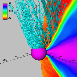
Figure 1: Field lines near a black hole rotating with $a/M=0.9$ hkh04 . The background colors illustrate matter density on a logarithmic scale, calibrated by a color bar found in the upper left-hand corner. The axes show Boyer-Lindquist radial coordinate.

We stressed earlier that the classical Blandford-Znajek model predicts the luminosity in terms of the radial component of the magnetic field on the horizon and the rotation rate of the field lines, but gives no guidance about how to estimate the former, and only a guess about the latter. In the Newtonian limit far from the innermost stable circular orbit, the field-strength is tightly coupled to the accretion rate because angular momentum conservation requires

$$-\int\,dz\,\langle B_{r}B_{\phi}\rangle\simeq{\dot{M}\Omega\over 2\pi}.$$ (52)

Close to the black hole, this relation remains correct as an order of magnitude estimator. Consequently, when the field is directly associated with accretion, its intensity near the black hole should be proportional to $\dot{M}$. Using simulation data, hk06 confirmed this expected proportionality, but found that spin matters, too:

$$\langle\frac{B^{2}}{8\pi}\rangle\simeq\frac{0.01}{1-a/M}\frac{\dot{M}c^{5}}{(GM)^{2}},$$ (53)

where the magnetic energy is measured in the fluid frame at the event horizon.

Despite the fact that the accretion flow sets the scale of magnetic intensity, the inertia of matter has little to do with field dynamics near the rotation axis. As already mentioned, any matter with even the angular momentum of the last stable orbit is excluded from a cone surrounding the axis. Within that cone, the field is force-free in the sense that $||B||^{2}/(4\pi\rho hc^{2})\gg 1$. However, it should also be recognized that simulations like those done to date are not able to define quantitatively just how large this ratio is. Precisely because the matter’s angular momentum makes the interior of the cone forbidden territory, any matter in the jet cone got there by some numerical artifact, either exercise of a code density floor or through numerical error associated with insufficient resolution of the extremely sharp density gradient at the centrifugal barrier. The enthalpy of the gas is equally poorly known, but that is because the treatment of thermodynamics in global simulations thus far is so primitive. Thus, the most one can say at this point is that, in a purely qualitative sense, the interior of the jet cone should be magnetically dominated. For exactly these reasons, the Lorentz factor of the outflow is equally ill-determined.

Although even defining a field line rotation rate for time-dependent non-axisymmetric fields is a bit dicey, it is possible to do so in an approximate way by monitoring the azimuthal velocity of the matter attached to the field lines, and subtracting off the portion attributable to sliding along the field lines. For example, if one defines the “transport velocity” by $V^{i}\equiv u^{i}/u^{t}$, in Boyer-Lindquist coordinates the local field line rotation rate $\omega$ can be written as

$$\omega=V^{\phi}-B^{\phi}{V^{r}B^{r}g_{rr}+V^{\theta}B^{\theta}g_{\theta\theta}\over(B^{r})^{2}g_{rr}(B^{\theta})^{2}g_{\theta\theta}}.$$ (54)

As Fig. 2 shows, after averaging radially, the rotation rate is close to the MacDonald-Thorne guess, perhaps 10–$20\%$ less, with surprisingly little variation in polar angle through the jet mg04 ; hk06 .

Figure 2: Radially- and time-averaged local field line rotation rate (solid curve) as a function of polar angle for a simulation in which the black hole has spin parameter $a/M=0.95$ hk06 . The dotted curve is half the black hole’s rotation rate, the dash-dot curve is half the rotation rate of the inner boundary of the simulation, which is slightly outside the event horizon.

Strikingly, even when the accreting matter orbits opposite the sense of rotation of the black hole, the field lines in the jet rotate with the black hole, not the matter hk06 . This fact makes it clear that the primary motive power for the jet is drawn from the black hole, not matter circulating deep inside the ergosphere to which the field lines are attached.

Normalized to the rest-mass accretion rate in traditional fashion, the jet luminosity can be sizable when the black hole spins rapidly. Both mg04 and hk06 made rough analytic fits to the dependence on spin:

$$\eta_{\rm EM}\simeq\cases{0.068\left\{1+[1-(a/M)^{2}]-2\sqrt{1-(a/M)^{2}}\right\}&\hbox{\cite[cite]{\@@bibref{Authors Phrase1YearPhrase2}{mg04}{\@@citephrase{(}}{\@@citephrase{)}}}}\cr 0.002/(1-|a/M|)&\hbox{\cite[cite]{\@@bibref{Authors Phrase1YearPhrase2}{hk06}{\@@citephrase{(}}{\@@citephrase{)}}}}\cr}$$ (55)

Although these expressions do not agree precisely, they agree at a qualitative level: the efficiency can be $\sim 0.1$ at the highest spins, but is much smaller for $|a/M|<0.9$. That the efficiency can be so high when the black hole spins rapidly is of some interest, given qualitative arguments (e.g., lop99 ) that the luminosities of jets driven directly by a black hole could never be significant.

Because the field lines in the jet rotate, it carries angular momentum as well as energy away from the black hole. The electromagnetic angular momentum delivered to infinity by the jet can be comparable to the conventional angular momentum brought to the black hole by accretion gsm04 ; hk06 ; bhk08 , particularly when the black hole spins rapidly. In fact, gsm04 argued that the electromagnetic angular momentum lost in the jet rises so steeply with black hole spin that it may limit $a/M$ to $\simeq 0.93$, a level considerably below the limiting spin proposed by t74 , who suggested that preferential capture of photons emitted by the disk on retrograde orbits would cap $a/M$ at $\simeq 0.998$.

6.2 A slightly more complicated case: the effect of field geometry

Beckwith et al. bhk08 explored other options for the magnetic field’s initial geometry beyond that of the simplest model, including: a pair of quadrupolar loops, one above and one below the plane, with their field directions coinciding on adjacent edges; a purely toroidal field; and a sequence of four dipolar loops, each rather narrow in radial extent. All of these were far less effective in terms of time-averaged jet luminosity than the large dipolar loop initial state: the quadrupolar case by two orders of magnitude, the toroidal by three!

The explanation for these strong contrasts changes with the geometric symmetry in question. Quadrupolar loops residing in a single hemisphere can rise buoyantly as a single unit and collapse, reconnecting with themselves. Jets arising from that kind of field therefore tend to be highly episodic, with only brief moments of high luminosity. Toroidal fields cannot produce poloidal field on scales larger than roughly the disk thickness, so their jets are always weak. A train of dipolar loops leads to a succession of jet-launching and jet-destruction events, separated in time by the difference in inflow times between their inner and outer edges.

6.3 Open questions

Before directly applying the results of this simplest model to black holes in Nature, we must first answer several questions about its generality.

Do zero net-flux simulations describe a steady-state jet?

Although these jets are long-lasting, they behave in certain ways as if the flux had been placed on the black hole as an initial condition (it arrives well before the accretion flow and then stays there, with little change). Moreover, although it may take a long time, eventually the far end of the large dipole loops must reach the black hole, and at that point reconnection will eliminate the field driving the jet. To gain a sense of the timescales involved, in the $\sim 10^{4}GM/c^{3}$ duration of these simulations, $\sim 10\%$ of the disk mass was accreted. One might guess, then, that the ultimate field annihilation would occur after $\sim 10^{5}GM/c^{3}$. For Galactic black hole binaries, this is only $\sim 5$ s; for AGN, it might be $\sim 5\times 10^{5}$–$5\times 10^{8}$ s, or no more than a few decades.

On the other hand, we do not know the true extent of such loops. It is at least conceivable that they might be much larger in radial extent, and the rapid increase of inflow time with radius might lead to much longer intervals between jet-field destruction events. If so, though temporary, these jets (especially in AGN) might be sufficiently long-lived as to be observationally interesting. Alternatively, one of the salient empirical facts about the jets we observe is that they are generally very unsteady. If another field loop follows close upon the heels of the one that just closed, the jet might be restored equally quickly. In this sense, the picture just described could give a better sense of the typical state of the jet.

What is the generic zero net-flux magnetic configuration?

Different zero net-flux magnetic geometries can lead to jets of drastically different character—how can we know which geometry (or mix of geometries) is present in any particular real object? It might seem “natural” to suppose that Nature is messy and serves up all possibilities at once, but when the different geometries differ in their results by orders of magnitude, the specific proportions matter a great deal. On the other hand, perhaps when the source of the accretion flow is a relatively ordered structure (e.g., a companion star in a binary system), the magnetic field delivered to the black hole, even while possessing no net flux, might be predominantly of a single topological character. One might speculate (as did bhk08 ) that changes in the predominant topology might be related to observable changes in jet strength, for example, as seen in galactic black hole binaries.

What would be the effect of net magnetic flux?

Major open questions also remain in regard to a different sort of ill-understood magnetic geometry: the possible presence of large-scale magnetic field threading the accretion disk and possibly the immediate environs of the black hole. This is a very controversial issue: advocates exist for almost the entire range of possible answers, from very large to nil. On the one hand, if the accreting gas is truly infinitely conductive, it should hold onto any large-scale field threading it and bring that flux to the event horizon of the black hole. Even if successive parcels carry oppositely-directed flux, the magnitude of the flux will have a non-zero expectation value $\sim\sqrt{N}\Phi$, where $N$ is the number of accumulated flux ropes and $\Phi$ is their typical individual magnitude tpm86 . On the other hand, when gas is accreted by a black hole, the characteristic length scale of variation for the magnetic field contained within it must shrink by many orders of magnitude. Severe bends must then be created in any field lines stretching to large distance, and extremely thorough reconnection may therefore be expected. In principle, all the field within the inner part of the accretion flow may lose contact with large-scale fields by this mechanism. Presumably, the correct story lies somewhere between these two extremes.

A sense of the range of views brought to bear on this problem may be gained by mentioning a few of the contending approaches. lpp94 attempted to define the problem in terms of the ratio between the accretion flow’s magnetic diffusivity and effective viscosity (in modern language, $\langle-B_{r}B_{\phi}\rangle/(6\pi\rho\Omega)$). They argued that this ratio, an effective magnetic Prandtl number, determines whether fields are locked to the accretion flow (and must therefore bend sharply as they leave the disk) or can slip backwards relative to the flow (and therefore stay pretty much where they started, without being forced to bend substantially). Unfortunately, the distance between this sort of “lumped parameter” approach and the actual microphysics is great enough that this approach hardly suffices to decide the issue. More recently, some (e.g. su05 ) have argued that clumps of flux could self-induce inflow by losing angular momentum through a magnetic wind, while others (e.g. rl08 ) have suggested that little net magnetic flux inflow would occur because turbulent resistivity inside the disk effectively disconnects large-scale field lines from the accretion flow in the interior of the disk. As this sampling of the literature indicates, the matter remains highly unsettled.

It is, however, potentially an important question because large-scale flux running through the disk could have important effects both on its accretion dynamics and on its ability to support a jet. Simulational studies of MHD turbulence in shearing boxes suggest that net vertical flux can strongly enhance the saturation level of the turbulence sits04 . How much of this effect is automatically embedded in global simulations by field loops that connect different radii remains unclear. In regard to jets, a consistent sense of vertical field would certainly serve to stabilize a base luminosity against the disruption that quadrupolar loops, etc. can create.

This issue could have significant observable consequences because the specific character of the large-scale field may depend strongly on black hole environment. One could well imagine that the field brought to the black hole by accretion from a stellar companion has more organized large-scale structure than the field threading turbulent interstellar gas accreting onto a black hole in a galactic nucleus. It is possible that long-term magnetic cycles in the companion star of a binary black hole system are connected to long-term changes in the state of the accretion flow and jet. There could even be cases intermediate between field entirely contained within the accretion flow and field with large-scale constraints: this might be the situation in a collapsing star in which extremely rapid accretion onto a nascent black hole drives a jet that creates a $\gamma$-ray burst bk08 .

Does the condition of the matter matter?

As remarked earlier, neither the density nor enthalpy of the matter in the jet can be determined quantitatively by simulations done to date. Although part of the difficulty is numerical, there are also serious unsolved physics (and astrophysical contextual) problems standing in the way. If there were, for example, a supply of matter with substantially smaller angular momentum than the matter in the accretion flow proper, it would see only a low centrifugal barrier and could enter the jet cone. Its thermal state would surely depend on whether there are numerous low-energy photons passing through the jet for the gas’s electrons to upscatter (as in the case of AGN) or very few (as in the case of a microquasar in a low-hard state). In the sort of collapsing star that might be the central engine for a $\gamma$-ray burst, the thermal state of gas in the vicinity of the jet would depend on its nuclear composition and the neutrino intensity. Although the launching of relativistic jets by black holes may be only weakly-dependent on the state of the matter it carries so long as $B^{2}/(4\pi\rho h)\gg 1$, the subsequent dynamics of the jet—its ultimate Lorentz factor, for example—are likely sensitive to these considerations.

7 Conclusions

Because work in this field is moving forward rapidly, any conclusions pronounced at this stage must be limited and preliminary. Nonetheless, results to date are certainly strong enough to give us some confidence that jet-launching mechanisms within the Blandford-Znajek conceptual family play a major role in this process. Magnetic fields that link distant regions with regions deep in the ergosphere have now been shown by explicit example to have the power, at least in principle, to tap the rotational energy of spinning black holes.

The progress that has been achieved so far rests on computational solutions of equations that, at least within the terms of the MHD approximation, express essentially ab initio physics. It is the direct connection to bed-rock physics (momentum-energy conservation, Maxwell’s Equations, etc.) that gives us confidence that their results are meaningful and robust. Greater contact with observations will become possible when the physics contained in these calculations is expanded to include better descriptions both of how matter enters the jet and of how it couples to radiation. Although it will be difficult to build foundations for these parts of the problem as securely-based as those of the dynamics, it may yet be possible to do so at a level permitting some reasonable testing by comparison with real data.

References

- (1) S.A. Balbus, J.F. Hawley: RMP 70, 1
- (2) J.M. Bardeen, W.H Press, S.A. Teukolsky: Ap.J. 178, 347 (1972)
- (3) M.V. Barkov, S.S. Komissarov: M.N.R.A.S. 385, L28 (2008)
- (4) K.R.C. Beckwith, J.F. Hawley, J.H. Krolik: Ap.J. 678, 1180 (2008)
- (5) V.S. Beskin, I.V. Kuznetsova: Il Nuovo Cimento B 115, 795 (2000)
- (6) R.D. Blandford, R.D., R.L. Znajek: M.N.R.A.S. 179, 433 (1977)
- (7) J.-P. De Villiers, J.F. Hawley: Ap.J. 589, 458 (2003)
- (8) J.-P. De Villiers, J.F. Hawley, J.H. Krolik, S. Hirose: Ap.J. 620, 878 (2005)
- (9) C.R. Evans, J.F. Hawley: ApJ 332, 659 (1988)
- (10) S. Fromang, J. Papaloizou, G. Lesur, T. Heinemann: A& A 476, 1123 (2007)
- (11) C.F. Gammie, J.C. McKinney, G. Tóth: Ap.J. 589, 444 (2003)
- (12) C.F. Gammie, S.L. Shapiro, J.C. McKinney: Ap.J. 602, 312 (2004)
- (13) J.F. Hawley, J.H. Krolik: Ap.J. 641, 103 (2006)
- (14) S. Hirose, J.H. Krolik, J.F. Hawley: Ap.J. 606, 1083 (2004)
- (15) Komissarov, S., arXiv:0804.1912 (2008)
- (16) J.H. Krolik, J.F. Hawley, S. Hirose: Ap.J. 622, 1008 (2005)
- (17) M.M. Kuznetsova, M. Hesse, L. Rastätter, A. Taktakishvili, G. Tóth, D.L. De Zeeuw, A. Ridley, T.I. Gombosi: J.G.R.A 112, 10210 (2007)
- (18) M. Livio, G.I. Ogilvie, J.E. Pringle: 1999 Ap.J. 512, 100 (1999)
- (19) S.H. Lubow, J.C.B. Papaloizou, J.E. Pringle: M.N.R.A.S. 267, 235 (1994)
- (20) D. MacDonald, K.S Thorne: M.N.R.A.S. 198, 345 (1982)
- (21) J.C. McKinney, C.F. Gammie: Ap.J. 611, 977 (2004)
- (22) S.C. Noble, J.H. Krolik, J.F. Hawley: submitted to Ap.J. (2008)
- (23) R. Penrose: Riv. Nuovo Cimento 1, 252 (1969)
- (24) E.S. Phinney: A Theory of Radio Sources, PhD thesis, Cambridge University, Cambridge UK (1983)
- (25) B. Punsly, F.V. Coroniti: Ap.J. 350, 518 (1990)
- (26) D.M. Rothstein, Lovelace, R.V.E.: Ap.J. 677, 1221 (2008)
- (27) T. Sano, S. Inutsuka, N.J. Turner, J.M. Stone: Ap.J. 605, 321 (2004)
- (28) H.C. Spruit, D.A. Uzdensky: Ap.J. 629, 960 (2005)
- (29) J.M. Stone, M.L. Norman: Ap.J.Suppl. 80, 753 (1992)
- (30) M. Takahashi, S. Nitta, Y. Tatematsu, A. Tomimatsu: Ap.J. 363, 206 (1990)
- (31) K.S. Thorne: Ap.J. 191, 507 (1974)
- (32) K.S. Thorne, R.H. Price, D.A. MacDonald: Black Holes, The Membrane Paradigm, Yale University Press: New Haven (1986)
- (33) G. Tóth: J.Comp.Phys. 161, 605