Deterministic remote preparation of arbitrary photon polarization states

Abstract

We propose a deterministic remote state preparation scheme for photon polarization qubit states, where entanglement, local operations and classical communication are used. By consuming one maximally entangled state and two classical bits, an arbitrary (either pure or mixed) qubit state can be prepared deterministically at a remote location. We experimentally demonstrate the scheme by remotely preparing 12 pure states and 6 mixed states. The fidelities between the desired and achieved states are all higher than 0.99 and have an average of 0.9947.

I introduction

Quantum information science brings us into a whole new era, so that the information can be manipulated and processed with quantum mechanical systems. One of the remarkable exhibitions of the fascination of quantum information science is quantum teleportation teleportation , which can transmit an unknown state from one location to another without sending a physical copy of the initial state. Remote state preparation (RSP), which is another significant application of entanglement, has been proposed recently lorsp ; patirsp ; bennettrsp . Unlike teleportation, however, in RSP Alice (the sender) knows completely the desired state. Alice is supposed to help Bob (the receiver) prepare the desired state at a remote location with the aid of her complete knowledge of the desired state, prior shared entanglement and classical communications.

In recent years, RSP has attracted much attention, and various approaches towards RSP have been studied experimentally with varying degrees of control over remotely prepared qubits. Using liquid-state NMR, remote preparation of pseudopure states is experimentally realized firstly NMRrsp . Since then, the experimental remote preparation of several kinds of constrained states have also been reported rsp2 ; rsp3 ; rsp4 ; rsp5 . RSP can even be realized with classical correlations instead of quantum correlations (i.e., entanglement) ccsrsp . Recently, arbitrary remote control of single-qubit state have been experimentally realized petersrsp ; prsp ; liursp ; atomicrsp . In Ref. petersrsp , the trigger photon and the remote photon are entangled in a Bell state, thus projection measurement on the trigger photon in a basis which contains the desired state will project the remote photon into the desired state or a state orthogonal to the desired state. Due to the impossibility of a universal NOT operation on arbitrary qubit states NOT , the efficiency for remote preparation of pure states are only 50%. The efficiencies for remote preparation of mixed states depends on the desired state, and are at least 50%. The efficiency can be 100% only if the desired state is constrained to lie on a single great circle on the Poincaré sphere. In Ref. prsp , the efficiencies for remote preparation of arbitrary qubit states (including pure states and mixed states) also depend on the desired state, which are at least 50%. In Ref. atomicrsp ; liursp , both the polarization and the spatial mode of the photon are considered. Polarization beam splitter (PBS) acts as CNOT logic gate between the polarization (control qubit) and spatial (target qubit) for complete Bell-state measurement BSM1 ; BSM2 ; BSM3 . The efficiencies for remote preparation of arbitrary pure states in Ref. atomicrsp ; liursp are 100% at the cost of precisely controlling two interferometers note . The efficiency for remote preparation of mixed states in Ref. liursp remain 50% owing to the impossibility of a universal NOT operation. Thus far, to our best knowledge, there is no RSP implementation which realize remote preparation of arbitrary single-qubit states (including pure states and mixed states) deterministically.

In this paper, we report the first experimental demonstration of deterministic remote preparation of arbitrary single-photon polarization states, where entanglement, local operation and classical communications (LOCC) are employed. By virtue of positive operator-valued measures (POVM), we can realize deterministic remote preparation of arbitrary pure states at a cost of one entanglement bit (ebit) and two classical bits (cbits). By combining POVM and controlled decoherence, we can also achieve deterministic remote preparation of arbitrary mixed states. The communication costs are the same as that in remote preparation of pure states. Furthermore, instead of two Mach-Zehnder interferometers in Ref. atomicrsp ; liursp , only one interferometer is needed in our scheme. This kind of simplification makes our scheme more feasible and executable in possible practical applications. In order to evaluate the performance of our scheme, we remotely prepare 12 pure states and 6 mixed states. The fidelities between the desired and achieved states are all higher than 0.99 and have an average of 0.9947.

II Theoretical Protocol

II.1 Deterministic implementation of arbitrary POVM on single-photon polarization state

POVM on single-photon polarization state plays a crucial role in our RSP protocol. So it would be the best to start from the deterministic realization of arbitrary POVM on single-photon polarization state with linear optics elements.

POVM is the most general class of quantum measurement kraus , which can be described by a collection of operators $\{M_{m}\}$. The subscript m labels the possible measurement outcomes. If the system state to be measured is described by a density matrix $\rho$, then after the measurement the system state becomes

$$\rho_{m}=\frac{M_{m}\rho M_{m}^{\dagger}}{tr(M_{m}^{\dagger}M_{m}\rho)},$$ (1)

and the corresponding probability is given by $p_{m}=tr(M_{m}^{\dagger}M_{m}\rho)$. The measurement operators $\{M_{m}\}$ satisfy the completeness equation $\sum_{m}M_{m}^{\dagger}M_{m}=I$, where $I$ is unit matrix. If we define that $E_{m}\equiv M_{m}^{\dagger}M_{m}$, then $E_{m}$ will be a positive operator and $\sum_{m}E_{m}=I$. The operators $E_{m}$ are called POVM elements of the measurement and the complete set $\{E_{m}\}$ is called a POVM quantuminformation .

As discussed in Ref. ET , the module sketched in Fig. 1 can be used to implement arbitrary two-outcome POVM on single-photon polarization state. The main part of the module is an interferometer consisted of two polarizing beam splitters (PBS) and the relative phase between two arms is zero. Two variable polarization rotators (VPR) in the interferometer controls the polarization state in path state $|p_{1}\rangle$ or $|p_{2}\rangle$ respectively. The module also contains unitary operator $V$ at the entrance of the interferometer, unitary operator $U_{1}$ at the exit $q_{1}$ and unitary operator $U_{2}$ plus NOT operator $X$ at the exit $q_{2}$.

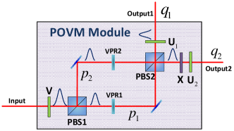
Figure 1: Schematic diagram of the module which can implement arbitrary two-outcome POVM on single-photon polarization state. PBS: polarizing beam splitters; VPR: variable polarization rotator; X: NOT operator. $V$, $U_{1}$ and $U_{2}$ are variable unitary operators.

Consider the case where $V=U_{1}=U_{2}=I$, and the polarization states in path state $|p_{1}\rangle$ and $|p_{2}\rangle$ are rotated as follows:

$$|H\rangle \xrightarrow{VPR1} \cos\zeta|H\rangle+\sin\zeta e^{i\theta}|V\rangle;$$

$$|V\rangle \xrightarrow{VPR2} \cos\xi|H\rangle+\sin\xi e^{i\sigma}|V\rangle.$$ (2)

If a state in the form of $|\varphi\rangle=a|H\rangle+b|V\rangle(|a|^{2}+|b|^{2}=1)$ enters the module shown in Fig. 1, the state evolves as

$$|\varphi\rangle\xrightarrow{} (a\cos\zeta|H\rangle+b\sin\xi e^{i\sigma}|V\rangle)|q_{1}\rangle$$ (3)

$$+(a\sin\zeta e^{i\theta}|H\rangle+b\cos\xi|V\rangle)|q_{2}\rangle.$$

If one measures the output states, the output of $|q_{1}\rangle$ and $|q_{2}\rangle$ correspond to matrices $D_{1}$ and $D_{2}$ respectively:

$$D_{1}=\left(\begin{array}[]{cc}\cos\zeta&0\\ 0&\sin\xi e^{i\sigma}\end{array}\right),D_{2}=\left(\begin{array}[]{cc}\sin\zeta e^{i\theta}&0\\ 0&\cos\xi\end{array}\right).$$ (4)

Note that $D_{1}^{\dagger}D_{1}+D_{2}^{\dagger}D_{2}=I$, so when $V=U_{1}=U_{2}=I$ any two-outcome POVM described by $D_{1}$ and $D_{2}$ can be realized with this module.

As we know, any square matrix A has its singular value decomposition. That means there exist unitary matrices $U$ and $V$, and a diagonal matrix $D$ with non-negative entries such that A=UDV. The diagonal elements of D are called the singular values of $A$ quantuminformation . So we represent the measurement operators $\{M_{1},M_{2}\}$ of arbitrary two-outcome POVM as: $M_{1}=U_{1}D_{1}V_{1},M_{2}=U^{\prime}_{2}D_{2}V_{2}$. The moduli of the elements of the diagonal matrix $D_{1}$ or $D_{2}$ are confined to lie between 0 and 1. As required by the completeness equation $E_{1}+E_{2}=I$,

$$E_{1}+E_{2} = V_{1}^{\dagger}D_{1}^{\dagger}D_{1}V_{1}+V_{2}^{\dagger}D_{2}^{\dagger}D_{2}V_{2}$$ (5)

$$= V_{1}^{\dagger}D_{1}^{\dagger}D_{1}V_{1}+V_{2}^{\dagger}(I-D_{1}^{\dagger}D_{1})V_{2}$$

$$= I+(V_{1}^{\dagger}D_{1}^{\dagger}D_{1}V_{1}-V_{2}^{\dagger}D_{1}^{\dagger}D_{1}V_{2})=I.$$

From Eq. (5), it is easy to prove that $V_{2}=WV_{1}$ where $W$ is only a diagonal unitary matrix. Notice that $W$ is commute with diagonal matrix $D_{2}$, so if we choose $V=V_{1}$ in the entrance, $U_{1}$ operator in the exit $q_{1}$ and $U_{2}=U^{\prime}_{2}W$ in the exit $q_{2}$, we can implement arbitrary collection of operators $\{M_{1},M_{2}\}$,

$$M_{1}=U_{1}\left(\begin{array}[]{cc}\cos\zeta&0\\ 0&\sin\xi e^{i\sigma}\end{array}\right)V,M_{2}=U_{2}\left(\begin{array}[]{cc}\sin\zeta e^{i\theta}&0\\ 0&\cos\xi\end{array}\right)V.$$ (6)

It means the module shown in Fig. 1 can be used to realize arbitrary two-outcome POVM.

The realization of POVM in our module is deterministic rather than probabilistic. And any more complicated POVM may be implemented by making a cascade of such modules. Our design is similar to that in Ref. Ahnert2005 , however the complexity of the experimental setup is significantly reduced, which makes it easier to realize as shown in our experiment.

II.2 Deterministic RSP scheme for pure states

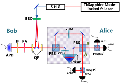
Figure 2: Experimental arrangement for remote preparation of pure states. SHG: second-harmonic generator; QP: quartz crystal; PA: polarization analyzer; IF: interference filter.

In our RSP protocol, we suppose that Alice and Bob share a maximally entangled photon pair of the form

$$|\psi_{AB}\rangle=\frac{1}{\sqrt{2}}(|H_{A}V_{B}\rangle+|V_{A}H_{B}\rangle),$$ (7)

where the subscripts (A,B) label Alice and Bob, $|H\rangle$ and $|V\rangle$ label horizontal and vertical polarization states of photons.

We start from remote preparation of pure states. Consider that the desired pure state is

$$|\varphi_{B}\rangle=\alpha|H_{B}\rangle+\beta e^{i\phi}|V_{B}\rangle.$$ (8)

Without loss of generality, we assume that $\alpha,\beta,\phi$ are real numbers, $\alpha^{2}+\beta^{2}=1$ and $\phi\in[0,2\pi)$. The experimental arrangement for remote preparation of pure states is sketched in Fig. 2. VPR1 and VPR2 are arranged to rotate the polarization component as follows:

$$|H\rangle \xrightarrow{VPR1} \alpha|H\rangle+\beta e^{i\phi}|V\rangle$$

$$|V\rangle \xrightarrow{VPR2} \alpha|H\rangle+\beta e^{i\phi}|V\rangle.$$ (9)

Then the POVM module in the shadowed box implement POVM described by:

$$M_{1}=\left(\begin{array}[]{cc}\alpha&0\\ 0&\beta e^{i\phi}\end{array}\right),M_{2}=\left(\begin{array}[]{cc}\beta e^{i\phi}&0\\ 0&\alpha\end{array}\right).$$ (10)

After the POVM measurement, the initial entangled state (7) becomes

$$\alpha|H_{A}V_{B}\rangle+\beta e^{i\phi}|V_{A}H_{B}\rangle$$ (11a)

$$or\ \ \ \alpha|H_{A}H_{B}\rangle+\beta e^{i\phi}|V_{A}V_{B}\rangle,$$ (11b)

depending on the measurement outcome (i.e., from which output port of the module Alice’s photon flies out).

The whole two-photon state now can be read as

$$|\Psi_{AB}\rangle= \frac{1}{2} [|D_{A}^{b}\rangle(\alpha|H_{B}\rangle+\beta e^{i\phi}|V_{B}\rangle)$$ (12)

$$+ |A_{A}^{b}\rangle(\alpha|H_{B}\rangle-\beta e^{i\phi}|V_{B}\rangle)$$

$$+ |D_{A}^{a}\rangle(\alpha|V_{B}\rangle+\beta e^{i\phi}|H_{B}\rangle)$$

$$+ |A_{A}^{a}\rangle(\alpha|V_{B}\rangle-\beta e^{i\phi}|H_{B}\rangle)],$$

where $|D\rangle\equiv(|H\rangle+|V\rangle)/\sqrt{2}$, $|A\rangle\equiv(|H\rangle-|V\rangle)/\sqrt{2}$ and the superscripts (a,b) label the output ports a and b (see Fig. 2).

The PBS($@45^{o}$) and the photon detectors (APD1-4) on Alice’s side fulfill the polarization projection measurement in the basis $\{|D_{A}\rangle,|A_{A}\rangle\}$ (see Fig. 2). Thus when Alice’s photon is projected onto $\langle D|(\langle A|)$, Bob’s photon is remotely prepared in one of the four states which is the desired state or a state up to an elementary correction operator. According to Alice’s measurement outcomes, Bob performs local unitary operation $\hat{I}$, $\hat{\sigma}_{z}$, $\hat{\sigma}_{x}$ or $\hat{\sigma}_{y}$ to obtain the desired state. Tuning three parameters in Eq. (II.2), arbitrary pure states can be remotely prepared deterministically. The classical information cost is 2 cbits with four possible results.

II.3 Deterministic RSP scheme for mixed states

Combined with POVM that allows us to remotely prepare arbitrary pure states deterministically, controlled decoherence allows us to realize deterministic remote preparation of arbitrary mixed states. The experimental arrangement for remote preparation of mixed states is sketched in Fig. 3, which is the same as that in Fig. 2 apart from the additional VPR and the decoherer.

Consider that the desired mixed state is

$$\rho_{B}=p^{2}|\varphi_{B}\rangle\langle\varphi_{B}|+q^{2}|\varphi^{\bot}_{B}\rangle\langle\varphi^{\bot}_{B}|\\$$

with

$$|\varphi_{B}\rangle=\alpha|H_{B}\rangle+\beta e^{i\phi}|V_{B}\rangle,\ \ \ |\varphi^{\bot}_{B}\rangle=\beta e^{-i\phi}|H_{B}\rangle-\alpha|V_{B}\rangle,$$ (13)

and $\langle\varphi_{B}|\varphi^{\bot}_{B}\rangle=0$. Without loss of generality, we assume that $p,q$ are real numbers, $p^{2}+q^{2}=1$, and $\alpha,\beta,\phi$ are the same as before. To prepare arbitrary mixed states we need to achieve complete control over all five parameters. VPR1 and VPR2 shown in Fig. 3 are arranged to rotate the polarization component as follows:

$$|H\rangle \xrightarrow{VPR1} p|H\rangle+q|V\rangle$$

$$|V\rangle \xrightarrow{VPR2} p|H\rangle+q|V\rangle.$$ (14)

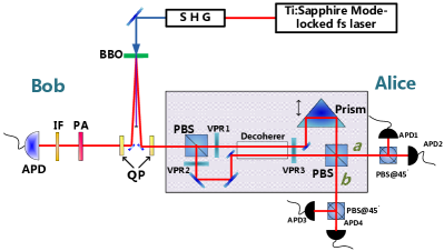
Figure 3: Experimental arrangement for remote preparation of mixed states. SHG: second-harmonic generator; QP: quartz crystal; PA: polarization analyzer; IF: interference filter.

A 20-mm-long quartz rod is inserted into both arms of the interferometer. With the fast axis of the quartz rod oriented horizontally, the birefringent element introduces $\sim 650fs$ delay between the V-polarized component and the H-polarized component, which is larger than the photon’s coherence time (given by $\lambda^{2}/(c\cdot\Delta\lambda)\sim 240fs$ in our experiment). VPR3 is arranged to rotate the polarization component in both arms as follows:

$$|H\rangle \xrightarrow{VPR3} \alpha|H\rangle+\beta e^{i\phi}|V\rangle$$

$$|V\rangle \xrightarrow{VPR3} \beta e^{-i\phi}|H\rangle-\alpha|V\rangle.$$ (15)

Then POVM measurement described by $M_{1}$ and $M_{2}$ are performed on both the V-polarized component and the H-polarized component.

In principle, the states can be distinguished by the different arrival time of the photon with different polarization. However, the effective coincidence window used in the experiment is $\sim 1ns$, which is much more larger than the time delay between the distinguishable states ($\sim 650fs$). In this way, we trace over the timing information during state detection to erase coherence between these distinguishable states, which is equivalent to irreversible decoherence ericsson ; decoherence . Thus, we finally obtain the polarization-entangled mixed state

$$p^{2}|\psi_{1}\rangle_{AB}\langle\psi_{1}|+q^{2}|\psi_{3}\rangle_{AB}\langle\psi_{3}|$$ (16a)

$$or\ \ \ p^{2}|\psi_{2}\rangle_{AB}\langle\psi_{2}|+q^{2}|\psi_{4}\rangle_{AB}\langle\psi_{4}|$$ (16b)

depending on POVM measurement outcome, with

$$|\psi_{1}\rangle_{AB} = \alpha|H_{A}V_{B}\rangle+\beta e^{i\phi}|V_{A}H_{B}\rangle$$

$$|\psi_{2}\rangle_{AB} = \alpha|H_{A}H_{B}\rangle+\beta e^{i\phi}|V_{A}V_{B}\rangle$$

$$|\psi_{3}\rangle_{AB} = \beta e^{-i\phi}|H_{A}V_{B}\rangle-\alpha|V_{A}H_{B}\rangle$$

$$|\psi_{4}\rangle_{AB} = \beta e^{-i\phi}|H_{A}H_{B}\rangle-\alpha|V_{A}V_{B}\rangle.$$

Then the PBS($@45^{o}$) and the detectors on Alice’s side perform the same projection measurement as before, which projects Bob’s photon onto one of the four mixed states:

$$\hat{\rho}_{B}^{I} = p^{2}|\varphi_{B}\rangle\langle\varphi_{B}|+q^{2}|\varphi^{\bot}_{B}\rangle\langle\varphi^{\bot}_{B}|$$

$$\hat{\rho}_{B}^{X} = p^{2}(\hat{\sigma}_{x}|\varphi_{B}\rangle)(\langle\varphi_{B}|\hat{\sigma}_{x})+q^{2}(\hat{\sigma}_{x}|\varphi^{\bot}_{B}\rangle)(\langle\varphi^{\bot}_{B}|\hat{\sigma}_{x})$$

$$\hat{\rho}_{B}^{Y} = p^{2}(\hat{\sigma}_{y}|\varphi_{B}\rangle)(\langle\varphi_{B}|\hat{\sigma}_{y})+q^{2}(\hat{\sigma}_{y}|\varphi^{\bot}_{B}\rangle)(\langle\varphi^{\bot}_{B}|\hat{\sigma}_{y})$$

$$\hat{\rho}_{B}^{Z} = p^{2}(\hat{\sigma}_{z}|\varphi_{B}\rangle)(\langle\varphi_{B}|\hat{\sigma}_{z})+q^{2}(\hat{\sigma}_{z}|\varphi^{\bot}_{B}\rangle)(\langle\varphi^{\bot}_{B}|\hat{\sigma}_{z}),$$ (17)

So Bob obtain the desired mixed state or a mixed state up to an elementary correction operator. According to Alice’s measurement outcome, Bob performs local unitary operation $\hat{I}$, $\hat{\sigma}_{z}$, $\hat{\sigma}_{x}$ or $\hat{\sigma}_{y}$ to achieve the desired mixed state. Notice that an arbitrary mixed states can be remotely prepared by tuning five parameters in Eq. (II.3) and the classical communication required is 2 bits.

III experiment and results

Our initial states (7) are generated with spontaneous parametric down conversion (SPDC). As shown in Fig. 2 and Fig. 3, a 1-mm-thick $\beta$-barium borate (BBO) crystal is pumped by UV laser pulses with 425 nm center wavelength and $\sim$ 530 mW average power from a frequency-doubled mode-locked Ti:Sapphire laser with $\sim$ 200 fs pulse duration and 76 MHz repetition rate. The photons obtained in degenerate, non-collinear type-II phase matching SPDC process are prepared in the state of Eq. (7) after the quartz crystals compensate the birefringence effects in BBO kwiat95 . We perform Clauser-Horne-Shimony-Holt (CHSH) inequality test on the entangled state and find that $S=2.6640\pm 0.0103$($|S|\leq 2$ for any local realism theory) CHSH .

For both pure and mixed states, PBS($@45^{o}$) at the output ports of the POVM module are used to preform projection measurement on Alice’s photon in the basis $\{|D\rangle,|A\rangle\}$. The photons are detected by single photon counting avalanche photodiode (SAPD) (Perkin-Elmer, SPCM-AQR-16) after an interference filter(10 nm FWHM). Coincidence (within a 1 ns time window) between Bob’s photon and corresponding trigger photon serves as classical communication. The coincidence circuit consists of a time-to-amplitude converter, a single-channel analyzer (TAC\SCA, ORTEC 567) and a universal time interval counter (Stanford Research Systems, SR620).

In our experiment, high visibility and long stable duration of the interferometer are crucial to the achievement of high fidelities. As shown in Fig. 2 and Fig. 3, the prism is utilized to compensate the path length difference (i.e., the relative phase) between two arms of the interferometer. The motor stage loading the prism is an ultra-precision linear motor stage (Newport, XMS50), and the resolution is below 1 nm which is precise enough for the compensattion of the path length difference.

The interferometer is located in a box fixed on an air cushion table to reduce the phase fluctuation. The visibility of the interferometer can maintain above 97% for several minutes which makes it possible to accomplish the whole tomography process and obtain high fidelities. The relative phase between two arms should keep being zero during the remote preparation process, otherwise the fidelity would dramatically decreased. So before the remote preparation of pure states, we insert a polarizer ($@45^{\circ}$) at the entrance of the POVM module. If the relative phase adjusted by the prism is set to be zero, the output state of the POVM module should be $|\varphi\rangle=\alpha|H\rangle+\beta e^{i\phi}|V\rangle$. The polarization analyzer (PA) at the output ports are used to perform projection measurement on the output polarization state in a basis $\{|\varphi\rangle,|\varphi^{\perp}\rangle\}$. If the visibility $(N_{\varphi}-N_{\varphi^{\perp}})/(N_{\varphi}+N_{\varphi^{\perp}})$ is near 100 %, we can make sure that the relative phase is near zero and the POVM module preforms the POVM operators in Eq.(10). Because the interferometer can maintain high visibility for several minutes, now we take off the polarizer and set the PA to measure in the basis $\{|D\rangle,|A\rangle\}$, then the stabilization time left is enough for the qubit tomography at Bob’ side. The manipulation of the POVM module in remote preparation of mixed states is similar. In our experiment the interferometer was not actively stabilized, however, we believe that active stabilization of the interferometer should be employed in practical applications.

In remote preparation of mixed states, the time delay introduced in one arm should be as exactly same as that in another arm. So that we can make sure that POVM measurement are accurately performed on both the foregoing H-polarized component and the following V-polarized component. To guarantee this, we use one quartz rod instead of two quartz rods to introduce the time delay on both arms (see Fig. 3), which avoid the length disagreement between any two quartz rods due to the manufacturing tolerance. Then both polarization components can perfectly interfere simultaneously and measurement operators $\{M_{1},M_{2}\}$ can be performed precisely on both components.

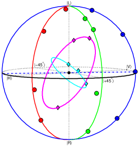
Figure 4: States remotely prepared in our experiment are shown in the Poincaré sphere. States are supposed to lie on the (semi)circle with the same color. The pure states are marked by circle and the mixed states are marked by diamond.

To evaluate the performance of our deterministic preparation scheme, we prepared 18 different states on Bob’s photon which include four pure states along each of three random longitude of the Poincaré sphere and six mixed states in the Poincaré sphere (see Fig. 4). With the tomography system on Bob’s side, we perform complete polarization analysis on the prepared polarization states. The results are converted to the closest physically valid density matrix using a maximum likelihood technique tomography . We use the fidelity $F(\rho_{o},\rho_{B})\equiv|Tr(\sqrt{\sqrt{\rho_{B}}\rho_{o}\sqrt{\rho_{B}}})|^{2}$ to evaluate the agreement between the prepared state ($\rho_{o}$) and the desired state ($\rho_{B}$) fidelity . The mean fidelity over all 18 states with all four possible results is 0.9947 in our experiment, while F=1 means perfect match. And the fidelities of all states are above 0.99.

IV conclusions and discussions

In our experiment, POVM are employed to achieve deterministic remote preparation of arbitrary photon polarization states. In fact, the kernel of our scheme is the entanglement transformation from the initial state (7) to the two-photon output state (11) or (16). Once the desired entanglement transformation is realized deterministically, we just need to perform appropriate projection measurement on Alice’s photon and the remote preparation is accomplished deterministically, as shown in our experiment.

Although we discuss the qubits encoded in the polarization of photons in our scheme, the methods can be generalized to other situations. While photons are ideal carriers in transfer of qubits, the matter carrier (e.g., ions, atoms, quantum dots, or superconducting circuits) are especially suitable for storage and processing of qubits. The operations on Alice’s photon can be utilized to remote control other matter systems provided that the matter system is maximally entangled with Alice’s photon atomicrsp , which is valuable for future applications such as quantum repeater and quantum networks.

We experimentally demonstrate the scheme by remotely preparing 12 pure states and 6 mixed states. The fidelities between the desired and achieved states are all higher than 0.99 and have an average of 0.9947.

In conclusion, we propose a deterministic remote state preparation scheme for photon polarization qubit states, where entanglement, local operations and classical communication are used. An arbitrary qubit state can be prepared deterministically at a remote location by consuming one maximally entangled state and two classical bits. The fidelities between the desired and prepared states are all higher than 0.99 and have an average of 0.9947, which indicate the high reliability of our protocol. Moreover, the experiment arrangement is more compact than before with only one interferometer used, which makes it more feasible and executable in further practical applications of quantum information science.

- (1) C. H. Bennett, et al., Phys. Rev. Lett. 70, 1895 (1993).
- (2) H. K. Lo, Phys. Rev. A 62, 012313 (2000).
- (3) A. K. Pati, Phys. Rev. A 63, 014302 (2001).
- (4) C. H. Bennett, et al., Phys. Rev. Lett. 87, 077902 (2001).
- (5) X.-H. Peng, et al., Phys. Lett. A 306, 271 (2003).
- (6) S. A. Babichev, et al., Phys. Rev. Lett. 92, 047903 (2004).
- (7) E. Jeffrey, et al., New J. Phys. 6, 100 (2004).
- (8) M. Ericsson, et al., Phys. Rev. Lett. 94, 050401 (2005).
- (9) G.-Y. Xiang, et al., Phys. Rev. A 72, 012315 (2005).
- (10) W. Wu, et al., Opt. Comm. 281, 1751 (2008).
- (11) N. A. Peters, et al., Phys. Rev. Lett. 94, 150502 (2005).
- (12) W. Wu, et al., Int. J. Quantum Inf. to be published.
- (13) W. Rosenfeld, et al., Phys. Rev. Lett. 98, 050504 (2007).
- (14) W.-T. Liu, et al., Phys. Rev. A 76, 022308 (2007).
- (15) V. Buzek, M. Hillery, and R. F. Werner, Phys. Rev. A 60, R2626 (1999).
- (16) S. P. Walborn, et al., Nature (London) 440, 1022 (2006).
- (17) Y. F. Huang, et al., Phys. Rev. Lett. 93, 240501 (2004).
- (18) C. Schuck, et al., Phys. Rev. Lett. 96, 190501 (2006).
- (19) Due to lack of variable beam splitter, in Ref. liursp the authors use a fixed beam splitter and apply different attenuators in the interferometer to realize the preparation of different states, which limits the RSP to a certain subset of states and leads to reduction of the efficiency. An implementation of the variable beam splitter is to use an additional Mach-Zehnder interferometer as was done in Ref. atomicrsp , with the cost of precisely controlling one more interferometer.
- (20) K. Kraus, Lecture Notes: States, Effects and Operations. Springer, (1983).
- (21) M. A. Nielsen, I. L. Chuang, Quantum Computation and Quantum Information. Cambridge University Press, (2000).
- (22) W. Wu, et al., Opt. Comm. 282, 2093 (2009).
- (23) S. E. Ahnert, M. C. Payne, Phys. Rev. A 71, 012330 (2005).
- (24) M. Ericsson, et al., Phys. Rev. Lett. 94, 050401 (2005).
- (25) P. G. Kwiat, and B.-G. Englert, Science and Ultimate Reality. Cambridge University Press, (2004).
- (26) P. G. Kwiat, et al., Phys. Rev. Lett. 75, 4337 (1995).
- (27) J. F. Clauser, et al., Phys. Rev. Lett. 23, 880 (1969).
- (28) D. F. V. James, et al., Phys. Rev. A 64, 052312 (2001).
- (29) R. Jozsa, J. Mod. Opt. 41, 2315 (1994).