Delayed Feedback Control Requires an Internal Forward Model

Abstract

Biological motor control provides highly effective solutions to difficult control problems in spite of the complexity of the plant and the significant delays in sensory feedback . Such delays are expected to lead to non trivial stability issues and lack of robustness of control solutions. However, such difficulties are not observed in biological systems under normal operating conditions. Based on early suggestions in the control literature, a possible solution to this conundrum has been the suggestion that the motor system contains within itself a forward model of the plant (e.g., the arm), which allows the system to ‘simulate’ and predict the effect of applying a control signal. In this work we formally define the notion of a forward model for deterministic control problems, and provide simple conditions that imply its existence for tasks involving delayed feedback control. As opposed to previous work which dealt mostly with linear plants and quadratic cost functions, our results apply to rather generic control systems, showing that any controller (biological or otherwise) which solves a set of tasks, must contain within itself a forward plant model. We suggest that our results provide strong theoretical support for the necessity of forward models in many delayed control problems, implying that they are not only useful, but rather, mandatory, under general conditions.

1 Introduction

The motivation for this work arose from biological motor control, which is plagued by inherent delays arising in sensory pathways, central processing units and motor outputs [4, 10]. However, the results established shed light on any feedback control system, subject to observation delays. Such delays, which in primates may reach 200-300 ms for visually guided arm movements, are very large compared to fast (150 ms) and intermediate (500 ms) movements [4, 10], and may lead to significant difficulties, as inappropriate control might cause instability or degraded performance. Delays have historically played a minor role in the field of robotics, as they can usually be made extremely small in such engineering applications. However, delayed state feedback has become increasingly important in engineering fields such as chemical control, distributed system control [16] and multisensory tracking [3]. In fact, one of the first attempts within the biological motor control literature [12] to address these issues was based on a well known concept from control theory, namely the Smith predictor [14]. However, one should keep in mind that in attempting to understand biological control systems, based on control theoretic principles, one is in fact trying to ‘reverse engineer’ an unknown system, as opposed to the task facing an engineer, namely designing a control system (see [18] for a survey of the possible role of control theory in systems biology).

Within an optimal control based approach, one needs to specify a class of admissible control laws, a set of plant constraints (e.g., musculo-skeletal), and a quantitative definition of performance, typically formulated in terms of a cost function. An optimal control law is then derived by minimizing a cost function subject to the relevant constraints. However, within a biological context, the precise nature of the plant and the controller is seldom known precisely, and the cost function used by the system (if indeed one is used), may also be unknown. It would thus be useful to determine general conditions for the necessity of a forward model, which require as few assumptions as possible. While a solution to the delay problem in the form of a forward model is indeed plausible and intuitively appealing [14], the question arises as to whether it is mandatory, namely, is it possible to construct an optimal closed-loop control law which is not based on a forward model? As we show in this paper, the answer to this question is negative, under very mild and reasonable conditions. More specifically, we show that (under appropriate conditions) an optimal feedback control law based on delayed state observations, must incorporate within itself a forward model of the plant.

As far as we are aware, there is currently no general theory which provides precise conditions for which forward models are indeed necessary. Early work, mainly concerned with the linear case (e.g., [7, 11, 17]), suggested several approaches to delayed control problems, including the proposal that a predictive plant model is needed, as in [14]. For example, [11] showed that optimal control for linear systems based on minimizing a quadratic cost is obtained by cascading a Kalman filter and a least-mean square state predictor. Later work extended these results in various directions. For example, [17] suggested an approach to dealing with disturbance attenuation and [13], focusing on stability issues, extended these results to more general linear systems, showing that state prediction is indeed a necessary component of such controllers. A survey of many aspects of this work, circa 2003, appears in [8]. We note that much of this work has dealt with the design of actual controllers (often for linear systems and quadratic cost). As mentioned above, our perspective in this work is somewhat removed from controller design, as we are concerned with a reverse engineering problem. More concretely, we begin with an observed control system, operating effectively under conditions of delayed state observations, and demonstrate that any effective controller must contain a forward plant model. Since it is hard, in general, to make even qualitatively correct assumptions about the system (e.g., linearity of dynamics and quadratic cost), we attempt to provide the most general result possible.

Before proceeding to a detailed description of our results, we note that the notion of an internal model has played an important role in control theory also in other contexts. Francis and Wonham [6] were the first to show that stable adaptation (a.k.a. regulation) requires the existence of an internal model. Adaptation refers to a situation where the output of the system maintains a constant asymptotic value whenever the system is subject to inputs from some class of signals. Intuitively, such an internal model enables the system to ‘subtract’ external inputs, thereby eliminating their long term effect on the system. Recently, a powerful extension of this theory was proposed in [15], where it was demonstrated to hold under very general conditions, without requiring the split into a ‘plant’ and a ‘controller’ which was required in the original framework of [6]. Interestingly, this general theory has been applied to bacterial chemotaxis and shown to provide interesting novel insight in other biological situations as well.

In summary, our main contribution in this work is the establishment of precise mathematical conditions for generic deterministic delayed feedback control systems to possess an internal forward model (we comment on the extension to the stochastic setting in Section 4, but leave the full elaboration of this direction to future work). The generality of the results, and the nature of the conditions required for them to hold, set the stage for the development, and experimental verification, of a rigorous theory of delayed feedback control in biological systems.

The remainder of the paper is organized as follows. Section 2 presents an overview of the main results, outlining sufficient conditions for delayed feedback control systems to possess a forward model. Specifically, in section 2.1 we outline the problem, followed by a simple example in section 2.2 and a summary of the main results in section 2.3. In section 2.4 we apply the general ideas to linear systems with time optimal control and delayed state observations, while in section 2.5 we consider the problem of minimum jerk control. Section 3 contains precise mathematical definitions and full proofs of the main results, including a full analysis of two examples presented cursorily in section 2. Finally, in section 4 we summarize our results and present some open research questions.

2 Results

This section contains a relatively informal summary of our main results. Precise definitions, assumptions, theorems and proofs appear in section 3. We begin by presenting the problem formulation, followed by a description of conditions for which a forward model is mandatory. We will then use the general necessary conditions established to show that in linear time optimal control and minimum jerk optimal control, based on delayed state observations, a forward model is indeed required.

2.1 Problem definition

Figure 1 about here

Consider a system to be controlled, referred to as a plant. A plant is usually described by a state vector $x^{p}\in X\subseteq\mathbb{R}^{n}$. For example, in a 2-D motor control setting with joint torques as control inputs, the plant is a 2-D manipulator. Its state consists of a pair of joint angles and two velocities. Assuming that the joint angles take values in the range $[0,\pi]$, while the velocities can assume any real value, we have $X=[0,\pi]^{2}\times\mathbb{R}^{2}$. The plant state dynamics are typically given by a differential equation of the form

$$\dot{x}_{t}^{p}=A_{p}(x_{t}^{p},u_{t}),$$ (1)

where $x_{t}^{p}$ is the state of the plant at time $t$, $\dot{x}_{t}^{p}$ denotes the temporal derivative of $x_{t}^{p}$, $u_{t}\in U$ is the control at time $t$, chosen from a set of possible controls $U$, and $A_{p}$ is a function mapping the state and control to $\mathbb{R}^{n}$, namely $A_{p}:X\times U\rightarrow\mathbb{R}^{n}$. In the above example of a 2-D manipulator, assuming that the torque is bounded in magnitude by $1$, we have $U=[-1,1]^{2}$.

In this work we study controllers possessing a memory which, as we demonstrate, is essential in the case of optimal control with delayed observations. The memory of the controller at time $t$ can be conceived of as the controller’s state at time $t$. For example, it is well known [14] that when controlling a plant with delayed state observation of duration $D$, using the previous controls $\left\{u_{s}\right\}$ for $t-D\leq s\leq t$ can be useful in order to calculate the current state of the plant. In this case the controller’s memory can be described by a function $x_{t}^{c}(\cdot)$, where $x_{t}^{c}(\alpha)=u_{t-\alpha}$ for all $0\leq\alpha\leq D$, namely the delayed control.

In order to rigorously investigate the notion of a forward model and derive conditions for its existence, we quantify this notion mathematically in section 3.1; here we summarize the main ideas. In the deterministic delayed state feedback case considered here, we define a forward model by the ability of the controller to compute $x_{t}^{p}$, the exact state of the plant at time $t$, given the delayed observation $x_{t-D}^{p}$ and its memory $x_{t}^{c}(\cdot)$. This ability to predict the exact state of the plant is equivalent to the existence of a transformation $F$ such that

$$x_{t}^{p}=F(x_{t}^{c},x_{t-D}^{p})\,\qquad\qquad\textrm{(forward$\,$ model)}.$$ (2)

In order to clarify the definition, consider a situation when a controller does not possess a forward model. This occurs when the relevant information available to the controller at time $t$ does not suffice to determine the current plant state $x_{t}^{p}$ unambiguously. More precisely, based on the current relevant information, $(x_{t-D}^{p},x_{t}^{c})$, the controller cannot determine $x_{t}^{p}$. Note that the controller in our model has additional information beyond $(x_{t-D}^{p},x_{t}^{c})$ (see Figure 1); as we claim later, this is irrelevant to the estimation of the current state $x_{t}^{p}$.

The need for a forward model can be established for many scenarios such as regulation, tracking and optimal control, and the proof is similar for all. We therefore use a common notion of tasks to refer to all the above. An example of a task for a 2-D manipulator is reaching some point $x^{p*}$ on a plane within a prespecified period of time, or, alternatively, in minimum time. Another possible task would be holding the manipulator still for $10$ seconds. Clearly, one can envisage any number of such tasks. The set of all tasks of interest will be denoted by $X^{*}$. Tasks are fed to the controller sequentially, and it is assumed that each task can be performed for each initial state. Note that the system is assumed to be causal, thus the controller has access only to the current task that should be performed and not to future tasks. The system described, based on delayed state observations, is illustrated in figure 1. The solving set of control laws for task $x^{*}$, up to time $t$, is denoted by $U_{t}^{*}(x^{p},x^{*})$ where $x^{p}$ is the initial state of the plant.

We will show in the sequel that the ‘richness’ of the set of tasks $X^{*}$, and the corresponding control solutions $U_{t}^{*}(x^{p},x^{*})$ can make a difference, as to whether a controller solving the task must possess a forward model or not. For example, in section 2.2 we introduce a plant and a controller solving a linear time optimal problem. In the first case, where the set of target states is $X^{*}=[-1,1]$, we show that a forward model is indeed essential. However, in the case where the set of targets is limited to two values, $X^{*}=\{-1,1\}$, we give an example of memoryless controller, which does not possess a forward model, while still solving the optimal control problem perfectly (i.e., a forward model is not needed in this case).

Next, we introduce a switching process, $z_{t}$, which defines the times at which new tasks are specified. Each task is assumed to be fixed between two consecutive task initiations. A precise definition of the switching process can be found in section 3. A control law is then defined by

$$u_{t}=B_{c}\left(x_{t}^{*},z_{t},x_{t}^{c},\tilde{x}_{t-D}^{p}\right),$$ (3)

where $D$ is the observation delay, $x_{t}^{*}\in X^{*}$ is the task to be performed at time $t$, and $B_{c}$ is a given function. We have introduced the notation $\tilde{x}_{t-D}^{p}=x_{(t-D)_{+}}^{p},$ where $(x)_{+}=\max(0,x)$, in order to deal systematically with times $t<D$. In addition to the control signal itself, we consider the dynamics of the controller’s state (memory). One standard formulation is in terms of a differential equation,

$$\begin{cases}\dot{x}_{t}^{c}(\alpha)=A_{c}\left(x_{t}^{*},z_{t},x_{t}^{c},\tilde{x}_{t-D},\alpha\right)\\ x_{0}^{c}(\alpha)=D_{c}(x_{0}^{p},x_{0}^{*},\alpha)\end{cases},$$ (4)

where, $A_{c}$ and $D_{c}$ are given functions describing the dynamics and initial conditions respectively.

In the definition of a forward model, we stated that the relevant information available to the controller regarding the current state $x_{t}^{p}$ is $(x_{t-D}^{p},x_{t}^{c})$. The controller has additional information available at time $t$, consisting of $x_{t}^{*}$ and $z_{t}$. However, since a new task can be specified at any time (independently of the value of $x_{t}^{p}$), the current state $x_{t}^{p}$ cannot depend on these values.

2.2 Example - a simple linear time optimal control problem

Figure 2 about here

The abstract ideas introduced in the previous section are clarified through a simple example. Consider a linear one dimensional time optimal control problem, where the objective is to drive the plant (described by a single real-valued variable $x^{p}$), to a point $x^{*}\in X^{*}=X$ in minimum time. The plant dynamics are given by

$$\dot{x}_{t}^{p}=-x_{t}^{p}+u_{t}\qquad;\qquad u_{t}\in[-1,1]\,.$$ (5)

The minimum time cost function is given by

$$J(x^{p},x^{*})=\int_{0}^{\tau_{f}}1dt=\tau_{f}\,,$$ (6)

where $\tau_{f}$ is the first time for which $x_{t}^{p}=x^{*}$, and the initial state of the plant is $x^{p}$. Thus, the controller needs to minimize $J(x^{p},x^{*})$. The set of tasks here corresponds to reaching any state $x^{*}\in X$ in minimum time. It is obvious that if $X=[-1,1]$, all the tasks can be performed, and the optimal solution in this case is simple and given by $u_{t}=\mathrm{sgn}(x^{*}-x_{t}^{p})$. This is an example of a so-called bang-bang control, where the control switches between its extreme allowed values; see figure 2 for a graphical illustration.

Before proceeding to establish the existence of a forward model we summarize the gist of the argument. We start by assuming that a controller can solve a set of tasks $X^{*}$, based on delayed state observation. We then argue by contradiction that if the controller lacks a forward model, then one can find a specific task $x^{*}\in X^{*}$ such that the controller will not be able to perform the task correctly, in contradiction to the assumption. Notice that the existence of such a task is a system related issue that has nothing to do with delays or a specific “black box controller”, as will be explained in section 2.3 .

The argument for the necessity of a forward model in the present example proceeds as follows (precise statements and proofs appear in sections 3.2 and 3.3). Assume that we are provided with a black box controller, which performs the linear time optimal control task optimally, based on delayed state observations. We will show that such a controller must possess a forward model. Assume to the contrary that it does not, thus there exist two distinct states, $s^{1}$ and $s^{2},$ $s^{1}\neq s^{2}$, such that the controller cannot determine whether the plant is currently in state $x_{t}^{p}=s^{1}$ or $x_{t}^{p}=s^{2}$. In other words, the controller’s available information relevant to the current state, namely $(x_{t-D}^{p},x_{t}^{c})$, does not suffice to determine $x_{t}^{p}.$ This implies that there exist two trials (namely, two initial states, times $t_{1}$ and $t_{2}$ and histories of tasks) such that the available information for both is identical, namely $(x_{t_{1}-D}^{p},x_{t_{1}}^{c})=(x_{t_{2}-D}^{p},x_{t_{2}}^{c})$, and such that $x_{t_{1}}^{p}=s^{1}$ and $x_{t_{2}}^{p}=s^{2}$ where $s^{1}\neq s^{2}$. However, if we specify an identical new task at times $t_{1}$ and $t_{2}$, namely $(x_{t_{1}}^{*},z_{t_{1}})=(x_{t_{2}}^{*},z_{t_{2}})$, the controller will choose $u_{t_{1}}=u_{t_{2}}$ due to (3). On the other hand, consider the system dynamics (5), and choose $x_{t_{1}}^{*}=x_{t_{2}}^{*}=\left(s^{1}+s^{2}\right)/2$, assuming, without loss of generality, that $s^{1}<s^{2}$. Based on the exact solution $u_{t}=\textrm{sgn}(x^{*}-x_{t}^{p})$, the optimal controls are $u_{t_{1}}^{*}=u^{1*}=1$ and $u_{t_{2}}^{*}=u^{2*}=-1$. However, based on the assumption that the forward model does not exist, we have shown that $u_{t_{1}}=u_{t_{2}},$ which contradicts the “correct task performing” assumption. Thus, in this example, a forward model is indeed required.

In order to better understand the requirement for a forward model, we consider an example where such a model is not needed. Consider the example discussed above, but where the set of tasks (destination states) consists of only two points $X^{*}=\{-1,1\}$. In this case a simple memoryless controller such as $u_{t}=x_{t}^{*}$ is optimal, and clearly lacks a forward model. The reason for this is simple. When two states $s^{1}\neq s^{2}$ are given, one cannot find a task $x^{*}$ such that the controls from $s^{1}$ and $s^{2}$ will differ. The reason is that if $x^{*}=-1$, the controller has to use $u=-1$ and if $x^{*}=1$, it has to choose $u=1$ independently of the initial state. Intuitively, the controller is not required to know the exact state of the plant in order to be optimal (perform the task). This simple example and intuition will form the basis of our general proof in section 3.2.

2.3 General results

Having argued for the existence of a forward model in a simple linear example, we extend the results to a general setting. To do this, we need to specify when a controller works “well”. Such a controller should perform all possible sequences of tasks correctly, which means that at each time, $t_{i}$, where a new task is given, the control signal for the task should belong to the set of controls $U_{t_{i+1}-t_{i}}^{*}(x_{t_{i}}^{p},x_{t_{i}}^{*})$ performing the tasks correctly between the times $t_{i}$ and $t_{i+1}$. We will refer to such a system as a Correct Task Performing System (CTPS); a precise characterization is provided in definition 6. This definition, based on the assumption that the task can always be solved, allows one to build a state feedback controller easily. We show that under these circumstances, a “delayed state feedback controller” can be built as well. We refer the reader to Theorem 7 for a precise statement of the result.

The proof of Theorem 7 is based on building a controller that uses delayed observations, by defining the memory of the controller to be $x_{t}^{c}(\alpha)=u_{t-\alpha}$. Then, given the observation $x_{t-D}^{p}$ , the current state $x_{t}^{p}$ can be reconstructed by solving the differential equation for the plant with initial condition $x_{t-D}^{p}$, where the previous controls are taken from the memory. Once the real state $x_{t}^{p}$ is available, we can choose the control from the set $U_{t}^{*}$.

As demonstrated in the simple example presented in section 2.2, a forward model may not always be necessary. As shown in section 3.2, the necessity of a forward model can be demonstrated in situations where the problem is sufficiently ‘rich’. In the example above, when the task set is binary, namely $X^{*}=\left\{-1,+1\right\}$, no forward model was required, while if $X^{*}=\left[-1,+1\right]$ a forward model is indeed required. This idea of problem richness is formalized in section 3.2. We will refer to a problem as sufficiently ‘rich’ by saying that it does not contain Non Separable by Correct Task Performing (NSCTP) pairs of states; see definition 8 for a precise characterization. Intuitively, we say that a pair of states is NSCTP when for every task, the same correct control exists at time $0$ for both states (however, the control may differ for each task). The main contribution of this paper, Theorem 9, establishes the existence of a forward model when NSCTP pairs of states do not exist (i.e., the absence of NSCTP pairs of states is a sufficient condition for a forward model to exist).

As a specific illustration of this idea, let us look back at the example in section 2.2. We implicitly proved there that the system does not have NSCTP pairs of states by finding a task $x^{*}=\left(s^{1}+s^{2}\right)/2$, and showing that it leads to $u^{1*}=1$ and $u^{2*}=-1$. The existence of a forward model in this case (and in more general cases to be studied in the sequel) follows from theorem 9.

2.4 Linear time optimal control

We consider an optimal setpoint tracking problem within linear control theory. The objective here is to reach, from an arbitrary initial position, a predefined setpoint $x^{*}$ in minimal time. In this case $X^{*}=X=\mathbb{R}^{n}$.

The cost function $J$, penalizing for time expended on the task, is

$$J(x^{0},u,\tau)=\int_{0}^{\tau}1dt=\tau,$$ (7)

where the initial state is $x^{0}$. The plant’s linear dynamics are described by the ODE

$$\begin{cases}\dot{x}_{t}=Mx_{t}+Nu_{t}\\ x_{0}=x^{0}\end{cases}\qquad;\qquad u_{t}\in[-1,1]^{m}\,,$$ (8)

where $M$ and $N$ are matrices of dimensions $n\times n$ and $n\times m$ respectively. The results can be generalized to more complicated sets of controls. We use theorem 9 to provide sufficient conditions for the existence of a forward model in this case. This is done by showing that linear time optimal control with delayed state feedback has no NSCTP pairs of states, thereby fulfilling the necessary conditions of the theorem. The precise statement of this result is provided in Theorem 13.

The proof that the system has no NSCTP pairs of states is based on geometrical properties of accessible sets, and can be found in section 3.3. Using Theorem 13, the need for a forward model in the simple example presented in section 2.2 can be established trivially, since the matrices $M$ and $N$ are given by $M=-1$ and $N=1$, which leads to a normal system (a required assumption for theorem 13), and the set $X=[-1,1]$ satisfies the other assumptions needed.

2.5 Minimum Jerk Optimal Control

Many models for the control of human arm movements have been suggested in an attempt to explain experimental results. The minimum jerk model was probably the first approach to address these issues based on optimal control principles [5]. In this approach, a two degree of freedom manipulator endpoint is controlled on a plane by applying jerk (the third derivative of the position). The task that the system should perform is taking the plant from some initial state to a final state in time $T$, minimizing the total accumulated squared jerk. We show that such a problem, where $T$ is a part of the task, possesses no NSCTP pairs of states, and therefore by theorem 9, a CTPS controller based on delayed inputs must contain a forward model.

In this model the state consists of the end-point of the manipulator’s displacement, velocity and acceleration in a plane,

$$\underline{x}^{p}=\left(x,y,\dot{x},\dot{y},\ddot{x},\ddot{y}\right)^{\top}=\left(x,y,u,v,z,w\right)^{\top},$$ (9)

with dynamics

$$\dot{\underline{x}}^{p}=\left(\dot{x},\dot{y},\ddot{x},\ddot{y},\delta,\gamma\right)^{\top},$$ (10)

where $\delta$ and $\gamma$ are the controls, namely $\underline{u}=\left(\dddot{x},\dddot{y}\right)^{\top}=\left(\delta,\gamma\right)^{\top}.$ We define a task termed optimal setpoint tracking in constant time where the plant must be controlled so that it reaches some state $x^{p*}$, with zero velocity and acceleration, while optimizing a cost function $J$, when the initial state of the plant is $x$ and the time for reaching the goal is $T$ (which is itself part of the task). Therefore the task is given by $x^{*}=(x^{p*},T)$ and $x^{p*}\in\tilde{X}$, where

$$\tilde{X}=\{x\in X\;|\;u=v=z=w=0\}.$$ (11)

The cost function is

$$J(\underline{x}_{0}^{p},u,T)=\frac{1}{2}\int_{0}^{T}\left(\dddot{x}_{t}^{2}+\dddot{y}_{t}^{2}\right)dt,$$ (12)

with initial conditions $\underline{x}_{0}^{p}=\left(x_{0},y_{0},x_{d0},y_{d0},x_{dd0},y_{dd0}\right)^{\top}$ and boundary conditions $\underline{x}_{T}^{p}=\left(x_{T},y_{T},0,0,0,0\right)^{\top}=\underline{x}^{p*}.$

As was shown in [5], each coordinate, $x$ and $y$, can be computed separately and identically, and the solution for $x$ has the following form

$$x_{t}=a_{0}+a_{1}t+a_{2}t^{2}+a_{3}t^{3}+a_{4}t^{4}+a_{5}t^{5},$$ (13)

where the constants $a_{i}$ depend on $T$, on the initial conditions and on $x^{p*}$. Theorem 16 proves that for this system a forward model is indeed essential. The proof is based on theorem 9 after showing that the system has no NSCTP pairs of states.

Note that when $T$ is constant and is not a part of the control task, the system has an infinite number of NSCTP pairs, and a similar proof will not work because it relies on the absence of NSCTP pairs in the system. However, this does not imply that a forward model is not needed, but rather that higher order conditions may be required.

3 Methods and Detailed Proofs

In this section we rephrase, in a formal mathematical language, the ideas and results introduced and presented intuitively in section 2. We begin with several technical definitions which will be required in the sequel.

3.1 Basic definitions

Let $X\subseteq\mathbb{R}^{n}$ be a set of states and $U\subseteq\mathbb{R}^{m}$ the set of possible actions that the controller can choose from. We use an underline to denote the history of a dynamic variable between time zero and time $t$, e.g., $\underline{u}_{t}:\;[0,t]\rightarrow U$ and similarly for arbitrary times $[t_{1},t_{2}]$ we use $\underline{u}_{[t_{1},t_{2}]}:\;[t_{1},t_{2}]\rightarrow U$. Denote by $\mathcal{U}_{t}$ the set of possible piecewise continuous controls that can be selected up to time $t$, namely $\mathcal{U}_{t}\triangleq\left\{\underline{u}_{t}:\;\underline{u}_{t}\text{ is piecewise continuous on}\;[0,t]\right\}$. The plant is given in (1).

We introduce a set of tasks to be solved, and a set of controls which solve these tasks.

Definition 1.

Let $X^{*}$ be a set of tasks that need to be solved by the controller, and let $x^{*}$ be a specific task. The set of task solving controls, $U_{t}^{*}(x^{p},x^{*})$, consists of all piecewise continuous control laws, in the interval $[0,t]$, that lead to the performance of task $x^{*}$ when the initial condition is $x^{p}$.

In the case where the task is completed for $\tau<t$ , the remaining controls are arbitrary, namely $U_{[\tau,t]}^{*}=\mathcal{U}_{t-\tau}$. Since we consider situations where the controller executes a series of tasks, we define the switching task process.

Definition 2.

The switching tasks process $z_{t}$ is defined by $z_{t}\triangleq\sum_{i=0}^{\infty}\delta(t-t_{i}),$ where $t_{i}$ are the times at which the tasks are switched, and $\delta\left(\cdot\right)$ is the Dirac impulse function.

The controller is given by (3) and its state dynamics (memory) by (4). While other definitions of memory may be considered, we limit ourselves in this letter to the present formulation. We assume that the task definition process $x_{t}^{*}$ is constant between two task switches. It will be convenient in the sequel to assume that the state space contains all states reachable for any allowable control law.

Definition 3.

The set $X\subseteq\mathbb{R}$ is inescapable when for all initial conditions $x_{0}^{p}\in X$, and controls $\underline{u}_{t}\in\mathcal{U}_{t}$, the state at time $t$ remains in $X$, namely $x_{t}^{p}\in X$.

In principle, the task solving control laws are not necessarily continuous. We introduce a subset of continuous control laws.

Definition 4.

For any $\epsilon>0,$ the set $\tilde{U}_{\epsilon}^{*}(x_{t}^{p},x^{*})\triangleq\{\underline{u}_{\epsilon}\in U_{\epsilon}^{*}(x_{t}^{p},x^{*}):\;\underline{u}_{\epsilon}\,\mathrm{is\,continuous}\}$, consisting of all continuous task solving controls, is termed the continuous task solving control set.

Next, we formally introduce the idea of a forward model.

Definition 5.

A controller possesses a forward model when there exists a transformation $F$ such that for all times $t$, initial conditions $x_{0}^{p}$, switching sequences $\underline{z}_{t}$, and tasks $\underline{x}_{t}^{*}$, the state is given by $x_{t}^{p}=F(x_{t}^{c},\tilde{x}_{t-D}^{p})$ where $\tilde{x}_{t-D}^{p}=x_{(t-D)_{+}}^{p}$.

In section 3.2 we provide precise conditions that imply the existence of a forward model.

3.2 General Results

The present section is constructed as follows. Initially, a system (plant and controller) with good performance is defined (definition 6). We then show that such systems can be implemented even when the state observation is delayed (Theorem 7). Finally, whenever the problem is not too trivial (see definition 8), we show that the controller must possess a forward model (Theorem 9).

Several assumptions are required before proceeding to the main claims. We assume that all possible sequences of tasks in $X^{*}$ can be performed by a controller from any initial condition in $X$, and we also require that $X$ cannot be escaped by applying legal controls.

Assumption 3.1.

For each task $x^{*}\in X^{*}$ and initial state $x^{p}\in X$, a piecewise continuous solution exists, namely, for any value of $t$, $U_{t}^{*}(x^{p},x^{*})\neq\emptyset$ .

In the sequel we will compare two control laws in a small interval around $t=0$. In order to do so, based on the values of the controls at $t=0$, we need to assume the existence of a small interval over which the task solving controls are continuous. In other words, for each task $x^{*}\in X^{*}$ and state $x^{p}\in X$, there exists $\epsilon_{0}(x_{t}^{p},x^{*})>0$ s.t $\tilde{U}_{\epsilon_{0}}^{*}(x_{t}^{p},x^{*})\neq\emptyset$. The existence of such an interval follows directly from assumption 3.1.

Assumption 3.2.

The set $X$ is inescapable.

Given a “black box controller” satisfying certain conditions, we will demonstrate the existence of a forward model.

Assumption 3.3.

A task solving “black box controller”, which provides a piecewise continuous and continuous from the right control signal $u_{t}$, is given.

Next, we define a “correctly performing system”, namely a system which executes all possible sequences of tasks correctly.

Definition 6.

The controller, plant and task space constitute a Correct Task Performing System (CTPS) when for each $\underline{x}_{t}^{*},\,x_{0}^{p},\,t,\underline{\,z}_{t}$,

$$\underline{u}_{[t_{i},\min(t_{i+1},t)]}\in U_{\min(t_{i+1},t)-t_{i}}^{*}(x_{t_{i}}^{p},x_{t_{i}}^{*})\;\;\mathrm{for\,all}\,i\in\{j:\;t_{j}<t\}.$$

In other words, the controller always selects a signal $u_{t}$ solving the sequence of tasks.

At this point we show that if there exists a controller without delay that renders the system CTPS, then a controller with delay can render the system CTPS as well. The intuitive idea is that in a deterministic system, the state of the controller can store all past controls, and thereby simulate the plant in order to predict the current state.

Theorem 7.

Let $A_{p}$ be a deterministic plant as in (1) with state variable $x_{t}^{p}$. Then under assumptions 3.1 and 3.2, there exists a controller of the form (3) such that the system is CTPS.

Proof.

Define $FM_{D}(x_{0}^{p},\underline{u}_{[0,D]})$ to be the solution of the dynamics of the plant at time $D$, when the initial state of the plant is $x_{0}^{p}$ and the control until time $D$ is $\underline{u}_{[0,D]}$. Now, define the state of the controller at time $t$ to be

$$x_{t}^{c}(\alpha)=[t,u_{\alpha}^{*}]^{\top}\in\mathbb{R}^{m+1}\,,$$ (14)

where $u_{\alpha}^{*}$ is the correct control at time $\alpha$ for performing the task. Note the $u_{\alpha}^{*}$ can be defined even for $\alpha>t$ assuming that $x_{r}^{*}=x_{t}^{*}$ for $t<r<\alpha$ ($x^{*}$ does not change). In (14) we separate the first component of the control state (representing time) from the other components, and use $x_{t,1}^{c}(\alpha)$ for the former and $x_{t,2}^{c}(\alpha)$ for the remaining $m$-dimensional sub-vector consisting of $u_{\alpha}^{*}$. We also define a projection of $x_{t}^{c}$ on an interval $[a,b]$ to be $x_{t}^{c}[a,b]$. The state $x_{t}^{c}$ defined in (14) is obtained by the dynamics

$$\dot{x}_{t}^{c}(\alpha)=\left[\begin{matrix}1\\ I_{\alpha\geq x_{t,1}^{c}}(u_{\alpha}^{*}-x_{t,2}^{c}(\alpha))z_{t}\end{matrix}\right]\,,$$

where we recall the definition 2 of the switching sequence $\left\{z_{t}\right\}$ in terms of an impulse train. The future control is selected from the correct solution set of controls. More formally, defining $\tilde{D}=\min[x_{t,1}^{c},D]$, we set $\hat{x}_{t}^{p}=FM_{\widetilde{D}}\left(x_{t-\widetilde{D}}^{p},x_{t,2}^{c}[x_{t,1}^{c}-\widetilde{D},x_{t,1}^{c}]\right)$ and $\underline{u}_{[t,\infty)}^{*}\in U_{\infty}^{*}\left(\hat{x}_{t}^{p},x_{t}^{*}\right)$. In other words $\underline{u}_{[t,\infty)}^{*}$ is chosen from the correct solution set $U_{\infty}^{*}(\hat{x}_{t}^{p},x_{t}^{*})$ where $\hat{x}_{t}^{p}=x_{t}^{p}$ is the exact prediction of the current state using the forward model $FM$. For such a definition of the memory, the control can be chosen by

$$u_{t} = B^{c}(x_{t}^{*},z_{t},x_{t}^{c},\tilde{x}_{t-D})$$

$$= x_{t,2}^{c}\left(x_{t,1}^{c}\right)\,.$$

It is obvious that the control between task switches is chosen so that $u_{[t_{i},t_{i+1}]}$ belongs to the set $U_{t_{i+1}-t_{i}}(x_{t_{i}}^{p},x_{t_{i}}^{*})$ for each $i$, and therefore it is CTPS. ∎

Next we introduce a property whereby two states may be “united” in terms of the solution to tasks, and therefore cannot be distinguished. For such states, for each task, there exists a continuous control such that controls at time $0$ are equal. The absence of such pairs will enable us to guarantee the existence of a forward model in a controller.

Definition 8.

For a problem where assumption 3.1 holds, a pair of distinct states $x^{p}$and $x^{\prime p}$, $x^{p}\neq x^{\prime p}$, is called a Non Separable by Correct Task Performing pair (NSCTP) if for all $x^{*}$, and $0<\epsilon<\min\{\epsilon_{0}(x^{p},x^{*}),\epsilon_{0}(x^{\prime p},x^{*})\}$, there exist controls $u\in\tilde{U}_{\epsilon}^{*}(x^{p},x^{*})$ and $u^{\prime}\in\tilde{U}_{\epsilon}^{*}(x^{\prime p},x^{*})$ such that $u_{0}=u_{0}^{\prime}$.

The following theorem constitutes the main theoretical result in the paper. It provides sufficient conditions for the existence of a forward model in delayed state feedback control. A required condition is the absence of NSCTP pairs in the system.

Theorem 9.

Let $A_{p}$ be a deterministic plant as in (1), and assume that NSCTP pairs of states are absent from the system. Let $(x^{c},B_{c})$ be a controller with delayed state feedback which renders the system CTPS. Then, under assumptions 3.1, 3.2 and 3.3, there exists a forward model $F$ such that for each $t,$ any initial condition $x_{0}^{p}$, and history of tasks $(\underline{x}_{t}^{*},\underline{z}_{t})$,

$$x_{t}^{p}=F(x_{t}^{c},\tilde{x}_{t-D}^{p})\,.$$

Proof.

Assume that the system is CTPS and assume by negation that such a forward model $F$ does not exist. Therefore there exist times $t_{1}$ and $t_{2}$, controller states $x_{t_{1}}^{c}(\cdot)=x_{t_{2}}^{c}(\cdot)$, and plant states $\tilde{x}_{t_{1}-D}^{p}=\tilde{x}_{t_{2}-D}^{p}$ such that for some two trials $(x_{0}^{p},\underline{x}_{t_{1}}^{*},\underline{z}_{t_{1}},t_{1})$ and $(x_{0}^{\prime p},\underline{x}_{t_{2}}^{\prime*},\underline{z}_{t_{2}},t_{2})$ we get $x_{t_{1}}^{p}\neq x_{t_{2}}^{\prime p}$. But the controller of the form (3) chooses the action by the rule $u_{t}=B^{c}(x_{t}^{*},x_{t}^{c},z_{t},\tilde{x}_{t-D}^{p})$. Therefore, for each new task $x^{*}$ set at times $t_{1}$ and $t_{2}$ for the two trials (since the system is inescapable and a solution always exists), we have $u_{t_{1}}=u_{t_{2}}$ and since $u_{t}$ is continuous from the right and piecewise continuous, there exist $\epsilon_{0}>0$ such that $u_{t_{i}}$ are continuous on $[t_{i},t_{i}+\epsilon_{i}]$ for $i\in\{1,2\}$. Thus, from the assumption that the system is CTPS, it follows that for all $x^{*}$ and $0<\epsilon<\min(\epsilon_{0},\epsilon_{1}(x_{t_{1}}^{p},x^{*}),\epsilon_{2}(x_{t_{2}}^{p},x^{*}))$, $u_{[t_{1},t_{1}+\epsilon]}\in\tilde{U}_{\epsilon}^{*}(x_{t_{1}}^{p},x_{t}^{*})$ and $u_{[t_{2},t_{2}+\epsilon]}\in\tilde{U}_{\epsilon}^{*}(x_{t_{2}}^{p},x_{t}^{*})$ (it suffices to look at the continuous solutions since we know that the control signal is piecewise continuous for the “black box controller”). But this means that the pair of distinct states $x_{t_{1}}^{p}$ and $x_{t_{2}}^{\prime p}$ is NSCTP which leads to a contradiction with the assumption that no such states exist. ∎

3.3 Linear time optimal control

We consider two examples demonstrating the general claims established in section 3.2. We begin in the present section by considering a linear control problem where the task is defined as optimal setpoint tracking, introduced in section 2.4. The objective here is to minimize the time required to reach the desired state with linear dynamics and delayed observations. The formal task is described in definition 10. In order to simplify the notation, we will omit the superscript $p$ from $x^{p}$ in this section. Some background results required in this section, and alluded to below, are taken from [9].

Definition 10.

Let $X^{*}=X$ and $x^{*}\in X^{*}$. The task is an optimal setpoint tracking task when

$$U_{t}(x,x^{*})=\operatorname*{argmin}_{u,\tau|x_{\tau}=x^{*}}J(x,u,\tau),$$

namely, the controller must take the plant state from the initial state $x$ to the desired state $x^{*}$ while minimizing the cost function $J$.

The time optimal cost function and the dynamics are given in (7) and (8) respectively. Let $u_{[0,t]}$ be a given control law. Then it is well known that

$$x_{t}=X_{t}x^{0}+X_{t}\int_{0}^{t}X_{s}^{-1}Nu_{s}ds,$$ (15)

where the matrix $X_{t}$ is the solution of the system,

$$\dot{X_{t}}=MX_{t}\quad\mathrm{with}\quad X_{0}=I,$$

which can be written explicitly as $X_{t}=e^{tM}$.

The existence of a forward model in this case will be demonstrated under the following assumptions that are needed to prove the absence of NSCTP pairs of states, and to fulfill the assumptions of theorem 9.

Assumption 3.4.

The system is essentially normal (as defined on p. 65 in [9]). The term “essentially” implies that a property holds almost everywhere - except on a set with measure zero. For simplicity, the term “essentially” will be omitted from now on in the context of normal systems. The set $X$ is a controllable and inescapable set (see Section 2.1).

The general definition of a normal system is somewhat intricate. However, for a time independent linear system of the form (8), theorem 16.1 in [9] establishes that the system is normal if and only if for each $j=1,\ldots,m$ the vectors ${\color[rgb]{1,0,0}{\color[rgb]{0,0,0}N,MN^{j},\ldots,M^{n-1}N^{j}}}$ are linearly independent, where $N^{j}$ are the column vectors of the matrix $N$. The exact conditions on the matrices $M$ and $N$ needed for the set $X$ to be controllable and inescapable require further analysis. However, a condition such as stability of $M$ insures the existence of a set $X$ with $0\in X$, that will be both controllable and inescapable.

As stated above, the main results in the present section rely heavily on basic concepts and theorems from [9]. For ease of reference, we recall some basic notions.

Definition 11.

Let $K(t,x^{0})$ be the accessible set at time $t$, starting from $x^{0},$namely

$$K(t,x^{0})\triangleq\{x:\mbox{$\,$ there exists }u\mbox{ which steers from }x^{0}\mbox{ to }x\mbox{ at time \mbox{t}\}.}$$

The following two key observations about normal systems are taken from [9].

• For a normal system, $K(t,x^{0})$ is strictly convex, bounded and closed.

• For normal systems, an optimal control law always exists, is unique and is essentially determined by $u_{t}^{*}=\mathrm{sgn}(\eta^{T}X_{\tau^{*}}X_{t}^{-1}N)$ for $x^{0},x^{*}\in X$ , where $\eta$ is an outward normal to $K(t,x^{0})$ at $x^{*}$, and the trajectory $x_{[0,t]}^{*}$ is unique.

We begin by proving a basic lemma that establishes some properties that are required in order to show that the system does not possess NSCTP pairs of states. The lemma establishes geometric properties of two intersecting accessible sets. A sketch of the ideas underlying the lemma is presented in Figure 3.

Lemma 12.

Let $x^{1},x^{2}\in X$ and $x^{1}\neq x^{2}$, and define $\tau^{m}\triangleq\sup\left\{\tau:\;K(\tau,x^{1})\cap K(\tau,x^{2})=\emptyset\right\}$. Then under assumption 3.4:

1. $\tau^{m}<\infty$.

2. $K(\tau^{m},x^{1})\cap K(\tau^{m},x^{2})=\{x^{*}\}$.

3. There exists an outward normal $g$ to a supporting hyperplane to $K(\tau^{m},x^{1})$ at $x^{*}$ and $-g$ is an outward normal to a supporting hyperplane to $K(\tau^{m},x^{2})$ at $x^{*}$.

   Figure 3 about here

Proof.

For a normal system there exists an optimal control, namely for all $x^{0},x^{*}\in X$ there exists a $\tau$ (might be infinity) such that $x^{*}\in\partial K(\tau,x^{0})$ (by Theorems 14.1, 14.2, 15.1 and Corollary 15.1 in [9]). Define $L\triangleq K(\tau^{m},x^{1})\cap K(\tau^{m},x^{2})$.

Proof of 1: Assume by negation that $\tau^{m}=\infty$. We know also that $X=\lim_{\tau\rightarrow\infty}K(\tau,x^{1})=\lim_{\tau\rightarrow\infty}K(\tau,x^{2})$ from assumption 3.4. From the definition of $\tau^{m}$, under assumption that $\tau^{m}=\infty$ there must exist $x^{3}\in X^{\circ}$ such that for all $\tau<\infty$, $x^{3}\notin K(\tau,x^{1})$ (without loss of generality). If $\tau^{m}=\infty$, then there is no optimal control from $x^{1}$ to $x^{3}$ which contradicts the existence of time optimal solution. Therefore $\tau^{m}<\infty$.

Proof of 2: First let us show that $L\neq\emptyset$. Assume by negation that $K(\tau^{m},x^{1})\cap K(\tau^{m},x^{2})=\emptyset$. Since $K$ is closed, strictly convex and compact (from Lemma 12.1, Corollary 15.1 in [9] and $\tau^{m}<\infty$), the sets $K(\tau^{m},x^{1}),K(\tau^{m},x^{2})$ are strictly separable by a hyperplane $f(x)=a\cdot x+b$ i.e., there exists $\epsilon>0$ such that for all $y\in K(\tau^{m},x^{1})$ $f(y)<-\epsilon$, and for all $z\in K(\tau^{m},x^{2})$, $f(z)>\epsilon$ by Proposition 2.4.3 [19]. Define $\tau^{1}=\inf\{\tau:\;K(\tau,x^{1})\cap\{x:f(x)=-\epsilon\}\neq\emptyset\}$ and $\tau^{2}=\inf\{\tau:\;K(\tau,x^{2})\cap\{x:f(x)=\epsilon\}\neq\emptyset\}$. Notice that $K(\tau^{1},x^{1})\cap\{x:f(x)=-\epsilon\}$ contains at most a single point since $K$ is closed, strictly convex and an optimal control always exists. The same argument applies to $K(\tau^{2},x^{2})\cap\{x:f(x)=+\epsilon\}$. Therefore $K(\tau^{1},x^{1})\cap K(\tau^{2},x^{2})=\emptyset.$ It follows that also for $\tau^{0}=\min(\tau^{1},\tau^{2})$, we have that $K(\tau^{0},x^{1})\cap K(\tau^{0},x^{2})=\emptyset$. But $\tau^{0}>\tau^{m}$, and this contradicts the definition of $\tau^{m}$, therefore $L\neq\emptyset$.
Next we show that $L^{\circ}=\emptyset$ . Assume by negation that it is not and let $x\in L^{\circ}$. Therefore $x\in K^{\circ}(\tau^{m},x^{1})$ and $x\in K^{\circ}(\tau^{m},x^{2})$, but from the definition of $\tau^{m}$ for all $\epsilon>0$, $x\notin K(\tau^{*}-\epsilon,x^{1})$ or $x\notin K(\tau^{m}-\epsilon,x^{2})$ (without the loss of generality assume that $x\notin K(\tau^{m}-\epsilon,x^{1})$) and $K$ is monotonic in $\tau$. Therefore for all $M>0$, $x\in K^{\circ}(\tau^{m}+M,x^{1})$ which leads to a contradiction that there is no optimal control from $x^{1}$ to $x$ as should be by Theorem 15.1 and Corollary 15.1 in [9]. Therefore $L^{\circ}=\emptyset$.
Let us show that $L$ cannot include more than a single point. Since $L^{\circ}=\emptyset$ and $L$ is strictly convex, then if $x,x^{\prime}\in L$ and $x\neq x^{\prime}$ then a convex combination should be in $L$. But since $L$ is strictly convex , the convex combination cannot be on $\partial L$ or in the interior of $L$ since it is empty. Therefore $L$ can contain only a single point.
Summarizing the above, $L$ is not empty and can contain only a single point, therefore $L=\{x^{*}\}$.

Proof of 3: Define $K_{1}\triangleq K(\tau^{m},x^{1})$ and $K_{2}\triangleq K(\tau^{m},x^{2})$. Since $K_{1}^{\circ}\cap K_{2}^{\circ}=\emptyset$ and $K_{1},K_{2}$ are convex, we can use the separating theorem for $K_{1}^{\circ},K_{2}^{\circ}$ (Proposition 2.4.2 [19]). Thus there exists a $g\in\mathbb{R}^{n}$, $g\neq 0$, such that for all $x\in K_{1}^{\circ}$, $x^{\prime}\in K_{2}^{\circ}$, $g\cdot x\leq g\cdot x^{\prime}$. Now let $x_{n}\in K_{2}^{\circ}$ such that $x_{n}\rightarrow x^{*}$ thus $g\cdot(x-x_{n})\leq 0$ and therefore $g\cdot(x-x^{*})\leq 0$. Similarly, we find that $g\cdot(x^{\prime}-x^{\ *})\geq 0$. Since the functional $(g\cdot x)$ is continuous, the same is correct for $y\in K_{1},y^{\prime}\in K_{2}$, i.e $g\cdot(y-x^{*})\leq 0$ and $g\cdot(y^{\prime}-x^{\ *})\geq 0$. Thus $g,-g$ are outward normals to supporting hyperplanes $K_{1},K_{2}$ respectively. ∎

Using lemma 12 we will establish that the system does not possess NSCTP pairs of states, and thus the need for a forward model will follow from theorem 9.

Theorem 13.

Consider a linear normal system described by (8), and assume that a controller with delayed input renders the system CTPS for an optimal setpoint tracking task, where the cost function is given by (7). If $x_{t}^{c}$ is the memory state of the controller, and assumptions 3.3 and 3.4 hold, then there exists a forward model $F$ such that for each $t,$ any initial condition $x_{0}^{p}$, and history of tasks $(\underline{x}_{t}^{*},\underline{z}_{t})$,

$$x_{t}^{p}=F(x_{t}^{c},\tilde{x}_{t-D}).$$

Proof.

First notice that assumption 3.3 holds since we required the system to be controllable, and from Theorem 13.1 in [9], the minimizer exists. Thus the task can always be performed, and from the normality of the system it follows that the time optimal control reaching $x^{*}$ is bang-bang, which implies that $\tilde{U}_{\epsilon}$ is not empty. First we will show that the system has no NSCTP pairs of states, and then use theorem 9 to establish the existence of a forward model.

For a normal system, the time optimal control reaching $x^{*}$ is given by

$$u_{t}=\mathrm{sgn}(\eta^{T}X_{\tau^{*}}X_{t}^{-1}N),$$

where $\eta$ is an outward normal to a supporting hyperplane to $K(\tau^{*},x^{0})$ at $x^{*}$ (except on a set of measure 0). It is essentially unique (may differ over a set of times with measure 0) by Theorems 14.1, 14.2, 15.1 and Corollary 15.1 in [9]. Now, let $x^{1}$ and $x^{2}$ be two distinct points in $X$, then by lemma 12 there exists $x^{*}$ which is reachable from $x^{1}$ and $x^{2}$ in time $\tau^{*}=\tau^{m}$ (since $x^{*}\in\partial K(x^{1},\tau^{m})$ and $x^{*}\in\partial K(x^{2},\tau^{m})$) by time optimal control, and there exist outward normals $\eta_{1}=g$ and $\eta_{2}=-g$. Since $X_{t}$ does not depend on the initial conditions,

$$u_{t}^{1}=-u_{t}^{2}\neq 0,$$

$u_{t}$ is piecewise continuous and $u_{0}^{1}\neq u_{0}^{2}$. Therefore for an arbitrary $x^{1}$ and $x^{2}$ we have found $x^{*}$ such that the solution is unique and $u_{0}^{1}\neq u_{0}^{2}$ . Thus the system does not possess NSCTP pairs of states. We have shown that all the assumptions required for theorem 9 hold, and therefore there exists a forward model $F$ such that $x_{t}^{p}=F(x_{t}^{c},\tilde{x}_{t-D}).$ ∎

3.4 Minimum Jerk Optimal Control

In this example, the plant’s state, dynamics, control and cost functions are given in (9-12). The initial and terminal conditions are given in section 2.5. The solution trajectory is given in (13), where the constants $a_{i}$ are found using the initial and boundary conditions. Taking three derivatives of (13) and setting $t=0$, we obtain

$$\delta_{0} = \frac{60}{T^{3}}x_{T}-\frac{60}{T^{3}}x_{0}-\frac{36}{T^{2}}x_{d0}-\frac{9}{T}x_{dd0}.$$

First, notice that for a constant value of $T$, there exist NSCTP pairs. Each $\underline{x}=\left(x_{0},x_{d0},x_{dd0}\right)^{\top}$ and $\underline{x}^{\prime}=\left(x_{0}^{\prime},x_{d0}^{\prime},x_{dd0}^{\prime}\right)^{\top}$ such that

$$-\frac{60}{T^{3}}x_{0}-\frac{36}{T^{2}}x_{d0}-\frac{9}{T}x_{dd0}=-\frac{60}{T^{3}}x_{0}^{\prime}-\frac{36}{T^{2}}x_{d0}^{\prime}-\frac{9}{T}x_{dd0}^{\prime}$$

are NSCTP pairs (there are infinitely many of these) since for each $x_{T}$ the optimal control at time $0$ is

$$\delta_{0}(x_{T})=\delta_{0}^{\prime}(x_{T}).$$

This result does not imply that in the present case a forward model is not needed, but it does imply that a higher order condition may be required in order to prove it.

Assume then that the terminal time $T$ can vary. For this case we will prove in theorem 16 that a forward model is essential. First we will show in Lemma 15 that the system does not have NSCTP pairs of states, and then use theorem 9 to establish the claim.

Definition 14.

Let $X^{*}=\widetilde{X}\times$$\mathbb{R}$ , where $\tilde{X}\subseteq X$, and $x^{*}=\left(x^{p*},T\right)\in X^{*}$. The task is an optimal setpoint tracking in constant time task when

$$U_{t}^{*}(x,x^{*})=\operatorname*{argmin}_{u|x_{T}=x^{p*}}J(x,u,T),$$

namely, the controller must take the plant state from the initial state $x$ to the desired state in time $T$, while minimizing the cost function $J$.

In the present case the subset $\tilde{X}$ is given by (11).

Lemma 15.

The system (9) with dynamics (10) solving an optimal setpoint tracking in constant time task, and minimizing the cost function (12) has no NSCTP pairs of states.

Proof.

First, the control $(\delta,\gamma)$ is continuous, therefore $\tilde{U}_{T}^{*}(x_{t}^{p},x^{*})\subseteq U_{T}^{*}(x_{t}^{p},x^{*})$. The solutions are unique, therefore we just have to find a task $x^{*}$ where the controls at time 0 are different for 2 initials states.

Let $\underline{x}_{0}\neq\underline{x}_{0}^{\prime}$ be two initial states. Assume, without loss of generality, that the $x$ coordinate’s initial conditions are different in the two initial states, i.e., $\underline{x}=\left(x_{0},x_{d0},x_{dd0}\right)$ and $\underline{x}^{\prime}=\left(x_{0}^{\prime},x_{d0}^{\prime},x_{dd0}^{\prime}\right)^{\top}$ such that $\underline{x}\neq\underline{x}^{\prime}$. To show that the states are not a NSCTP pair we have to find $T$ and $x_{T}$ such that $\delta_{0}^{*}(x_{T})\neq\delta_{0}^{\prime*}(x_{T})$, where $\delta_{t}^{*}(x_{T})$ and $\delta_{t}^{\prime*}(x_{T})$ are the optimal controls to $x_{T}$ from the initial states $\underline{x}$ and $\underline{x}^{\prime}$ respectively. Recall that the optimal control at time $0$ is given by

$$\delta_{0}^{*}=\frac{60}{T^{3}}x_{T}-\frac{60}{T^{3}}x_{0}-\frac{36}{T^{2}}x_{d0}-\frac{9}{T}x_{dd0.}$$

The necessary and sufficient condition for equality of the controls $\delta_{0}^{*}(x_{T})=\delta_{0}^{\prime*}(x_{T})$ is

$$9(x_{dd0}-x_{dd0}^{\prime})T^{2}+36(x_{d0}-x_{d0}^{\prime})T+60(x_{0}-x_{0}^{\prime})=0.$$

Since this is a second order polynomial in $T$, there can be at most 2 roots $T_{1}$ and $T_{2}$. Let $\tilde{T}\neq T_{1},T_{2}$ and let $x_{\tilde{T}}$ be an arbitrary position, thus for $\tilde{T},x_{\tilde{T}}$, $\delta_{0}^{*}\neq\delta_{0}^{\prime*}$ which means that the pair of states $\underline{x}_{0}\neq\underline{x}_{0}^{\prime}$ are not a NSCTP pair. ∎

At this point we are ready to prove the existence of a forward model.

Theorem 16.

A “black box controller” with delayed state feedback fulfilling assumption 3.3 which renders system (9) with dynamics (10) CTPS for an optimal setpoint tracking in constant time task with cost function (12), must possess a forward model. In other words, there exists a forward model $F$ such that for each $t,$ any initial condition $x_{0}^{p}$, and history of tasks $(\underline{x}_{t}^{*},\underline{z}_{t})$,

$$x_{t}^{p}=F(x_{t}^{c},\tilde{x}_{t-D}^{p}).$$

Proof.

First, assumptions 3.1 and 3.2 hold trivially since the optimal trajectory is unique and continuous, and there exists a polynomial solution for each $x_{0}^{p}\in X$ and $x^{*}\in X^{*}$. From Lemma 15 we have that the system does not have NSCTP pairs, and therefore by Theorem 9 there exists a forward model $F$ such that for each $x_{0}^{p},\underline{x}_{t}^{*},t$

$$x_{t}^{p}=F(x_{t}^{c},\tilde{x}_{t-D}^{p}).$$

∎

4 Discussion

We have studied the general problem of control based on delayed state observations. For this purpose we have formalized the notion of a system solving a set of control tasks, which is general enough to cover many of the standard control settings such as regulation and tracking. Under rather mild conditions on the system, we have shown that such a controller must contain within itself a forward model. This implies that the current plant state can be exactly determined based on the delayed state observation and the internal controller state. We applied our general framework to two widely studied problems, linear time optimal control and minimum jerk control, and provided explicit conditions for the necessity of a forward model. These results, and the general framework itself, provide powerful mathematical support for the existence of forward models in biological motor control, and, in fact, in any control system with delayed feedback.

A possible limitation of our approach is its restriction to deterministic systems, as the notion of a forward model used here is clearly inapplicable in a stochastic setting. Since in a stochastic setting one cannot determine the state precisely, a reasonable requirement in this case is that the posterior state distribution, based on the observed delayed state and on previous controls, be determined from the present controller state. As was shown in [1], for additive cost functions the problem of control with delayed observations can be expressed as a Markov decision process without delay of a more complicated system. While we have obtained some results in this more challenging and realistic setting, the full elaboration of this issue is left for future work. A further open issue relates to approximate, rather than exact, task performance. We expect that in this case some notion of approximate forward model will play a role (e.g., [2]).

An interesting question relates to the necessity of the conditions we have provided, as we have only shown them to be sufficient. In fact, it is quite possible that milder conditions than the absence of NSCTP pairs suffice. Finally, it would clearly be of significant value to demonstrate the absence of NSCTP pairs, and thus the necessity of forward models, in more biologically relevant settings. However, proving this for nonlinear dynamical systems, with a level of complexity approaching that of biological systems, may require non-trivial analysis. We hope that simpler and mathematically more tractable conditions can be developed, whose existence will be easier to demonstrate.

Figure Captions

Figure 1 A delayed feedback control system, where the delayed plant state $x_{t}^{p}$ is observed by a controller. The sequence $x_{t}^{*}$ represents a set of tasks, and the sequence $z_{t}$ denotes the times at which tasks are switched.

Figure 2 A simple one-dimensional example where $X^{*}=X=[-1,1],\,U=[-1,1]$, and the objective is to drive the system to the point $x^{*}.$ The exact control solution in this case is $\mathrm{sgn}\left(x^{*}-x_{t}\right)$

Figure 3 Two accessible sets meet: The sets $K\left(\tau^{m},x^{1}\right)$ and $K\left(\tau^{m},x^{2}\right)$ intersect at time $\tau^{m}$ with the point $x^{*}$ at the intersection with the outward normals to the support hyperplane.

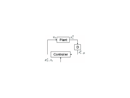
Figure 1:

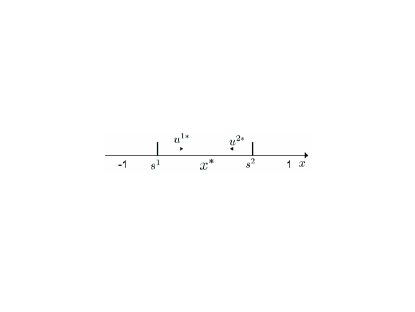
Figure 2:

|

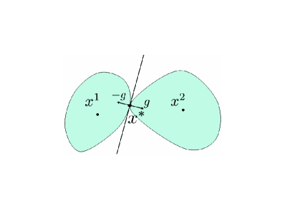
Figure 3:

References

- [1] E. Altman and P. Nain. Closed-loop control with delayed information. In acm sigmetrics Performance Evaluation Review, volume 20, pages 193–204. ACM New York, 1992.
- [2] B. Andrews, E.D. Sontag, and P. Iglesias. An approximate internal model principle: Applications to nonlinear models of biological systems. In In Proc. 17th IFAC World Congress, Seoul, 2008.
- [3] Y. Bar-Shalom. Update with out-of-sequence measurements in tracking: exact solution. IEEE Transactions on Aerospace and Electronic Systems, 38(3):769–778, 2002.
- [4] P.R. Davidson and D.M. Wolpert. Widespread access to predictive models in the motor system: a short review. J Neural Eng, 2(3):S313–S319, 2005.
- [5] T. Flash and N. Hogan. The coordination of arm movements: An experimentally confirmed mathematical model. Journal of Neuroscience, 5(7):1688–1703, 1985.
- [6] B. A. Francis and W. M. Wonham. The internal model principle for linear multivariable regulators. Applied Mathematics and Optimization, 2(2):170–194, 1975.
- [7] A.T. Fuller. Optimal nonlinear control of systems with pure delay. Int. J. Control, 8(2):145–168, 1968.
- [8] K. Gu and S.I. Niculescu. Survey on recent results in the stability and control of time-delay systems. ASME Journal of Dynamic Systems Measurement and Control, 125:158–165, 2003.
- [9] H. Hermes and Lasalle J. P. Functional Analysis and Time Optimal Control. Academic Press, Inc, 1969.
- [10] M. Kawato. Internal models for motor control and trajectory planning. Curr Opin Neurobiol, 9(6):718–727, 1999.
- [11] D.L. Kleinman. Optimal control of linear system with time-delay and observation noise. IEEE Trans Autom Control, 14(5):524–527, 1969.
- [12] R. Miall, D. Weir, D. Wolpert, and J. Stein. Is the cerebellum a Smith predictor? J Mot Behav, 25(3):203–216, 1993.
- [13] L. Mirkin and N. Raskin. Every stabilizing dead-time controller has an observer-predictor-based structure. Automatica, 39:1747–1754, 2003.
- [14] O.J.M. Smith. Closer control of loop with dead time. Chem Eng Progress, 53(5):217–219, 1957.
- [15] E.D. Sontag. Adaptation and regulation with signal detection implies internal model. Systems and Control Letters, 50:119–126, 2003.
- [16] S.C.A. Thomopoulos. Decentralized filtering and control in the presence of delays: discrete-time and continuous-time case. Information Sciences, 81(1-2):133–153, 1994.
- [17] K. Watanabe and M. Ito. A process-model for linear systems with delay. IEEE Trans Automatic Control, 26(6):1261–1269, 1981.
- [18] P. Wellstead, E. Bullinger, D. Kalamatianos, O. Mason, and M. Verwoerd. The role of control and system theory in systems biology. Annual reviews in Control, 32(1):33–47, 2008. n1392.
- [19] D. Bertsekas with A. Nedic and A.E Ozdaglar. Convex Analysis Optimization. Athena Scientific, 2003.