A Bijective Proof for Reciprocity Theorem

Abstract.

In this paper, we study the graph polynomial that records spanning rooted forests $f_{G}$ of a given graph. This polynomial has a remarkable reciprocity property. We give a new bijective proof for this theorem which has Prüfer coding as a special case.

1. Introduction

A spanning tree $T$ in some graph $G$ is a connected acyclic subgraph of $G$ that includes all vertices in $V(G)$. Calculating the number $t(G)$ of spanning trees for some graph $G$ is one of the typical questions we will ask. For example, when $G$ is a complete graph $K_{n}$, $t(K_{n})=n^{n-2}$. There are several methods to calculate $t(G)$, such as the matrix-tree theorem and Prüfer coding.

In this paper, we study some graph polynomial $f_{G}$ that records the spanning trees of the extended graph $\widetilde{G}$ of graph $G$. This polynomial can be used to compute the spanning tree of some complex graphs easily. For example, let $\Gamma=\Gamma\left(G;G_{1},\ldots,G_{k}\right)$ be the graph that is obtained by substitution of graphs $G_{1},\ldots,G_{k}$ instead of a vertices of a graph $G$. Then we can easily obtain $f_{\Gamma}$ by $f_{G}$ and $f_{G_{i}}$, for $1\leq i\leq k$.

In fact, the polynomial $f_{G}$ possess the remarkable property of reciprocity. A. Renyi [9] gives an inductive proof for this reciprocity theorem. I. Pak and A. Postnikov [1] also give an inductive proof. Throughout this paper, we present a new bijective proof for the reciprocity theorem. One interesting fact is that the map we used in the bijection is Prüfer coding when $G$ is a complete graph.

This paper is organized as follows: In section 2, we define the graph polynomial $f_{G}$ to enumerate spanning trees in $\widetilde{G}$. In section 3, we show the reciprocity theorem for $f_{G}$ and defined some tools for the future bijective proof. In section 4, we define two maps $\phi$ and $\psi$ to show the bijection between $\mathbf{A}$ and $\mathbf{B}$. Finally, in section 5, we use this bijective coorespondence to prove the reciprocity theorem of $f_{G}$.

2. Graph Polynomials for Spanning Trees

Suppose that $G=(V,E)$ is a graph with vertices $1,\ldots,n$, where $|V|=n$. Let $0\notin V$ and $\widetilde{V}:=V\cup\{0\}$. We say the extended graph $\widetilde{G}$ of $G$ is a graph on the set $\widetilde{V}$ obtained by adding edges $\{0,v\}$ to $G$ for all vertices $v\in V$. Clearly, if $G$ is a complete graph $K_{n}$ with $n$ vertices, then $\widetilde{G}$ is a complete graph $K_{n+1}$ with $n+1$ vertices. We denote the set of all spanning trees in $G$ as $\mathcal{T}_{G}$, i.e. all acyclic connected subgraphs in $G$ which contain all the vertices of $G$.

First of all, we assign variables $x_{i}$ to $i$, for all $1\leq i\leq n$. For any spanning tree $T$ in $\mathcal{T}_{G}$, define a function $m(T)$ associated to $T$:

$$m(T)=\prod_{v\in V}x_{v}^{\rho_{T}(v)-1},$$ (2.1)

where $\rho_{T}(v)$ denotes degree of the vertex $v$ in the tree $T$, i.e. the number of edges adjacent to the vertex $v$.

Now, we set the graph polynomial $t_{G}$ to be,

$$t_{G}:=\sum_{T\in\mathcal{T}(G)}m(T).$$

Let us associate the variable $x$ to vertex $0$. Then, the graph polynomial $f_{G}$ of variables $x$ and $x_{v}$, for all $v\in V$ is defined as follows:

$$f_{G}:=t_{\widetilde{G}}=\sum_{T\in\mathcal{T}_{\widetilde{G}}}m(T).$$ (2.2)

We denote $V=\{1,\ldots,n\}$ and $f_{G}=f_{G}(x;x_{1},\ldots,x_{n})$.

It is easy to see that the spanning trees in $\mathcal{T}_{\widetilde{G}}$ correspond to spanning rooted forests in $G$, i.e. acyclic subgraphs in $G$ containing all vertices in $V$, with a root chosen in each component. In particular, the two polynomials $t_{G}$ and $f_{G}$ possess the following identity:

$$t_{G}(x_{1},\ldots,x_{n})\cdotp(x_{1}+\cdots+x_{n})=f_{G}(0;x_{1},\ldots,x_{n}).$$ (2.3)

An short proof for Eq.(2.3) is provided in Igor Pak and A. Postnikov [1].

The graph polynomial $f_{G}$ has two important properties that allow us to compute the number of spanning rooted forests for certain graph. The first property is the composition of graphs. Let $G_{1}$ and $G_{2}$ be two graphs on disjoint sets of vertices, and $G_{1}+G_{2}$ be the disjoint union of the graphs. We associate variable $x$ to the root $0$, variables $y_{1},\ldots,y_{r_{1}}$ to the vertices of $G_{1}$, and variables $z_{1},\ldots,z_{r_{2}}$ to the vertices of $G_{2}$. Then the following formula holds:

$$f_{G_{1}+G_{2}}(x;y_{1}\ldots,y_{r_{1}},z_{1}\ldots,z_{r_{2}})=x\cdotp f_{G_{1}}(x;y_{1}\ldots,y_{r_{1}})\cdotp f_{G_{2}}(x;z_{1}\ldots,z_{r_{2}}).$$

One can prove the above equation by some simple arguments.

3. Reciprocity Theorem For Polynomials $f_{G}$

A graph $\overline{G}=(V,\overline{E})$ is called the compliment of some graph $G=(V,E)$ if $\overline{E}=\binom{V}{2}\backslash E$. That is to say, $e\in\overline{E}$ iff $e\notin E$. The graph polynomials $f_{G}$ possess the following reciprocity property:

$$f_{G}{(x;x_{1},\ldots,x_{n})}=(-1)^{n-1}\cdotp f_{\overline{G}}({-x-x_{1}-\cdots-x_{n};x_{1},\ldots,x_{n}}).$$ (3.1)

The case that $x_{1}=\cdots=x_{n}=1$ for (3.1) was found by S. D. Bedrosian [2] and A. Kelmans.

Before we give the bijective proof for Eq.(3.1), we first introduce some notation.

First of all, let $\acute{F}_{G}$ be a spanning tree of some extended graph $\widetilde{G}$ with root $0$ and vertices $1,\ldots,n$ so that $F_{G}$ is a spanning rooted forest of $G$. It is easy to show that for any vertex $u$ of $G$, there is a unique path from $u$ to root $0$. Therefore, we can assign a direction to every edge in $\acute{F}_{G}$ such that each arrow points toward the root $0$. This implies that every vertex $u\neq 0$ has outdegree 1. For convention, in this paper, when we say graphs $\acute{F}_{G}\in\mathcal{T}_{\widetilde{G}}$ or $F_{G}$, we always consider it as a directed graph, and thus for every $u\neq 0$, there is a unique directed edge $(u,v)\in E(\acute{F}_{G})$. In addition, a vertex $u$ is the child of vertex $u_{1}$ if there is a directed path from $u$ to $u_{1}$ in $\mathcal{T}_{\widetilde{G}}$.

Secondly, we say that a valid pair of some tree $\acute{F}_{K_{n}}$ is a pair $(u,v)\in F_{K_{n}}$, and $\mathbf{Z}_{G,\acute{F}_{K_{n}}}$ is a subset of valid pairs of $\acute{F}_{K_{n}}$ such that

$$\mathbf{Z}_{G,\acute{F}_{K_{n}}}=\{(u,v):(u,v)\notin E(\overline{G}),(u,v)\in E(F_{K_{n}})\}.$$ (3.2)

Now, given a subset $\mathbf{C}$ of all valid pairs not in $\mathbf{Z}_{G,\acute{F}_{K_{n}}}$, we define an operational set $\mathcal{O}_{G,\acute{F}_{K_{n}},\mathbf{C}}$ as follows:

$$\mathcal{O}_{G,\acute{F}_{K_{n}},C}=\mathbf{C}\cup\mathbf{Z}_{G,\acute{F}_{K_{n}}}.$$ (3.3)

One can see that for a spanning tree $\acute{F}_{K_{n}}$ and graph $G\in K_{n}$, there could be many possible operational sets. An example is in figure 1.

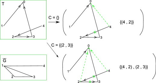
Figure 1. For $\acute{F}_{K_{n}}$ and $\overline{G}$ as above, we have two possible operational sets for $\acute{F}_{K_{n}}$. (The green marks are the graph after we apply all the pair in the operation sets to $\acute{F}_{K_{n}}$.)

Now, for any $\acute{F}_{\overline{G}}$, suppose its induced subgraph $F_{\overline{G}}$ in $K_{n}$ has $k$ connected components. We say a weight sequence $\mathcal{W}_{\acute{F}_{\overline{G}}}$ of $\acute{F}_{\overline{G}}$ is

$$\mathcal{W}_{\acute{F}_{\overline{G}}}=(w_{1},\ldots,w_{k-1}),$$ (3.4)

where $w_{j}\in\{0,1,\ldots,n\},\text{ for }1\leq j\leq k-1$. By convention, if $k=1$, we set $W_{T_{\widetilde{\overline{G}}}}$ to be empty. Therefore, there are $(n+1)^{k-1}$ possible weight sequences for spanning tree $\acute{F}_{\overline{G}}$ that has $k$ connected compoenents in $F_{\overline{G}}$.

Given a graph $G\in K_{n}$, let $\mathbf{A}$ be the set of all possible pairs $\left(\acute{F}_{K_{n}},\mathcal{O}_{G,\acute{F}_{K_{n}},C}\right)$ and $\mathbf{B}$ be the set of all possible pairs $\left(\acute{F}_{\overline{G}},\mathcal{W}_{\acute{F}_{\overline{G}}}\right)$. In the following section, we show a bijection between $\mathbf{A}$ and $\mathbf{B}$.

4. Bijection Between $\mathbf{A}$ to $\mathbf{B}$

Suppose that $G$ is a graph with $n$ vertices labeled $1,\ldots,n$ where each vertex $i$ is associated to a variable $x_{i}$, for $1\leq i\leq n$. For the root in the extended graph, we assign variable $x$ to root $0$. We first construct a map $\phi$ from $\mathbf{A}$ to $\mathbf{B}$.

Definition 4.1.

Given a pair $\left(\acute{F}_{K_{n}},\mathcal{O}_{G,\acute{F}_{K_{n}},C}\right)\in A$, the map $\phi$ outputs a pair $(\acute{F},\mathcal{W})$ and is defined as follows:

Let $S$ be the set of vertices $u$ in $\acute{F}_{K_{n}}$, where the directed edge $(u,v)\in E(\acute{F}_{K_{n}})$ is a pair in $\mathcal{O}_{G,\acute{F}_{K_{n}},C}$ or $v=0$. Construct an empty sequence $\mathcal{W}$ and a graph $\acute{F}$ which is a duplicate of $\acute{F}_{K_{n}}$.

WHILE $|S|>1$,

1:

Suppose there is a leaf $u^{\prime}\neq 0$ in $\acute{F}_{K_{n}}$ such that the edge $(u^{\prime},v^{\prime})\in E(\acute{F}_{K_{n}})$ is not in $S$. We remove $u^{\prime}$ and $(u^{\prime},v^{\prime})$ from $\acute{F}_{K_{n}}$.

2:

Repeat step 1 until every leaf $u\neq 0$ in $\acute{F}_{K_{n}}$ is also in $S$. Let $M$ to be the set of all these vertices.

3:

Delete the largest vertex $u^{*}$ in $M$ and the directed edge $(u^{*},v^{*})$ in $\acute{F}_{K_{n}}$. We set $S$ to be $S\backslash\{u^{*}\}$, and add $v^{*}$ to the end of the sequence $\mathcal{W}$.

4:

Remove edge $(u^{*},v^{*})$ and add edge $(u^{*},0)$ to $\acute{F}$.

RETURN $(\acute{F},\mathcal{W})$.

An example of this algorithm is in figure 2. In the following proposition, we prove that $\phi$ is well-defined.

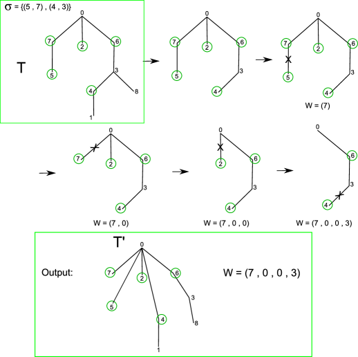
Figure 2. Input: $T=\acute{F}_{K_{n}}$ and $\mathcal{O}=\mathcal{O}_{G,\acute{F}_{K_{n}},C}=\{(5,7),(2,3)\}$, Output: $T^{\prime}=\acute{F}_{\overline{G}}$ and $\mathcal{W}=\mathcal{W}_{\acute{F}_{\overline{G}}}=\{7,0,0,3\}$

Proposition 4.2.

The map $\phi$ is a well-defined map from $\mathbf{A}$ to $\mathbf{B}$.

Proof.

It is easy to see that all the steps in WHILE loop work. Now, we show that $\acute{F}$ is a spanning tree of $\widetilde{K_{n}}$ after each step 4. We proceed this by induction.

Initially, $\acute{F}=\acute{F}_{K_{n}}$ is a tree. Suppose that at some step 4, we delete edge $(u^{*},v^{*})$ and add edge $(u^{*},0)$ to the spanning tree $\acute{F}\in\mathcal{T}_{\widetilde{K_{n}}}$. Furthermore, since for any vertex $u\neq 0$, $u$ and root $0$ is connected in graph $\acute{F}$, it remains connected after we change some edge $(u^{*},v^{*})$ to edge $(u^{*},0)$. Since $|E(\acute{F})|=n$, $\acute{F}$ is always a spanning tree of $\widetilde{K_{n}}$ after any step 4.

Now, from (3.3), we know that $\mathbf{Z}_{G,\acute{F}_{K_{n}}}\in\mathcal{O}_{G,\acute{F}_{K_{n}},C}$ and all the edges $(u,v)$ in the operational set $\mathcal{O}_{G,\acute{F}_{K_{n}},C}$ became $(u,0)$ in the output graph $\acute{F}$. Thus, every edge in $E(F)$ is also in $E(\overline{G})$, and $\acute{F}$ is a spanning tree of $\widetilde{\overline{G}}$.

Finally, we show that $W$ is a weight sequence of $\acute{F}$. Clearly, $S$ is the set of all roots in the spanning rooted forest $F$. Since the WHILE loop ends when $|S|=1$, there are totally $|S|-1$ elements added to the sequence $W$. Consequently, $W$ satisfies the length requirement in Eq.(3.4).

The above arguments tell us that $(\acute{F},\mathcal{W})\in B$ as desired. ∎

We now give a map $\psi$ from $\mathbf{B}$ to $\mathbf{A}$.

Definition 4.3.

Given a pair $\left(\acute{F}_{\overline{G}},\mathcal{W}_{\acute{F}_{\overline{G}}}\right)\in\mathbf{B}$, the map $\psi$ outputs $\left(\acute{F}^{*},\mathcal{O}\right)$ and is defined as follows:

Assume that the forest $F_{\overline{G}}$ has $k$ connected components and the associated weight sequence $\mathcal{W}_{\acute{F}_{\overline{G}}}=(w_{1},\ldots,w_{k-1})$. Create a tree $\acute{F}^{*}=\acute{F}_{\overline{G}}$, sequence $\mathcal{W}_{\acute{F}^{*}}=\mathcal{W}_{\acute{F}_{\overline{G}}}$, and an empty set $\mathcal{O}$. Let $R$ be the set of roots in $F_{\overline{G}}$.

WHILE the length of $\mathcal{W}_{\acute{F}^{*}}$ is larger than 0.

1:

We choose the first element $w$ in the sequence $\mathcal{W}_{\acute{F}^{*}}$. Let $u$ be the largest vertex in $R$ such that $w_{i}$ is not $u$ nor a child of $u$ in $\acute{F}^{*}$, for any $w_{i}$ in $\mathcal{W}_{\acute{F}^{*}}$. Delete the element $w$ from the sequence $\mathcal{W}_{\acute{F}^{*}}$ and $u$ from the set $R$.

2:

Remove the edge $(u,0)$ and add the edge $(u,w)$ to the graph $\acute{F}^{*}$. If $w\neq 0$, we add pair $(u,w)$ to the set $\mathcal{O}$, i.e. $\mathcal{O}=\mathcal{O}\cup\{(u,w)\}$.

RETURN $(\acute{F}^{*},\mathcal{O})$.

An example of this mapping $\psi$ is in figure 3. In the following lemma, we prove that $\psi$ is well-defined.

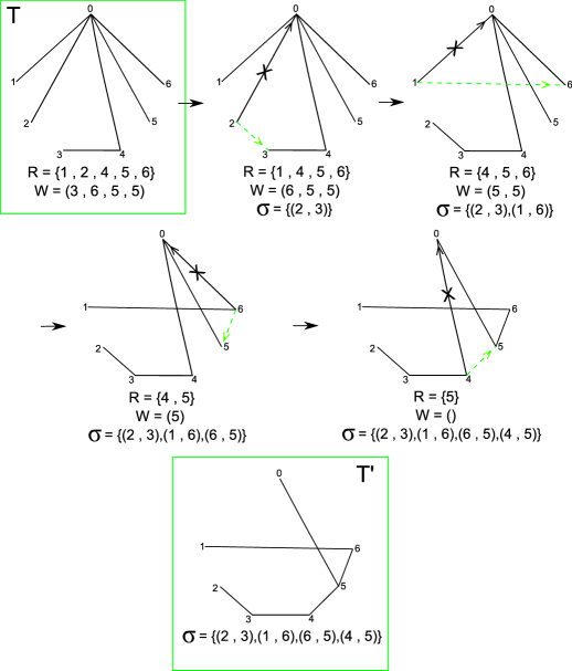
Figure 3. Input: $T=\acute{F}_{\overline{G}}$ and $W=\mathcal{W}_{\acute{F}_{\overline{G}}}=\{3,6,5,5\}$, Output: $T^{\prime}=\acute{F}^{*}$ and operational set $\sigma=\mathcal{O}=\{(2,3),(1,6),(6,5),(4,5)\}$. (R is the set of current roots.)

Proposition 4.4.

The map $\psi$ is a well-defined map from $\mathbf{B}$ to $\mathbf{A}$.

Proof.

We first show that at any stage, the set $R$ and graph $\acute{F}^{*}$ satisfy the following properties:

1. $\acute{F}^{*}$ is a spanning tree of $\widetilde{K_{n}}$, i.e. $F^{*}$ is a sapnning rooted forest of $K_{n}$.

2. $R$ is the sets of roots of forest $F^{*}$.

We proceed by induction on the number of loops. Initially, $R$ is the set of all the roots in forest $F_{\overline{G}}$, and $\mathcal{W}_{\acute{F}^{*}}$ is a sequence of length $k-1=|R|-1$. Moreover, at each step 1, we remove an element in $\mathcal{W}_{\acute{F}^{*}}$ and an element in $R$. Thus, the length of sequence $\mathcal{W}_{\acute{F}^{*}}$ is always $|R|-1$.

Now, suppose at some stage, we have that properties (1) and (2) hold and sequence $\mathcal{W}_{\acute{F}^{*}}=\{w^{\prime}_{1},\ldots,w^{\prime}_{k_{1}-1}\}$, where $k_{1}=|R|$. During step 1, since there are $k_{1}$ connected components in $F^{*}$, there exists at least one connected component that contains no elements in $\mathcal{W}_{\acute{F}^{*}}$. Consider the compoenent with the largest root $u$ that meets this condition. It is not hard to see that for any $1\leq i\leq k_{1}-1$, $w^{\prime}_{i}$ is not $u$ nor a child of $u$. Consequently, step 1 works.

For step 2, by the choice of vertex $u$, we have $w^{\prime}_{i}$ and $u$ are not connected in $F^{*}$. Suppose $\acute{F}^{*}$ becomes cyclic after we delete edge $(u,0)$ and add edge $(u,w^{\prime}_{1})$ to this graph. This implies that there is a cycle containing edge $(u,w^{\prime}_{1})$. It is not possible since vertices $u$ and $w^{\prime}_{1}$ would be connected in $F^{*}$ before we add edge $(u,w^{\prime}_{1})$.

The above arguments show that after step 1 and 2, $\acute{F}^{*}$ remains acyclic, and is a spanning tree of $\widetilde{K_{n}}$. Futhermore, after step 2, since $u$ is no longer a root, $R$ remains as the set of all roots in $F^{*}$. As a result, properties (1) and (2) always hold.

Finally, we need to show that $(v,v^{\prime})\in\mathcal{O}$, for every directed edge $(v,v^{\prime})\notin E(\overline{G})$ and $(v,v^{\prime})\in E(F^{*})$. Clearly, $\acute{F}^{*}$ is obtained from $\acute{F}_{\overline{G}}$ by a series of removing and adding edges in step 2. If edge $(v,v^{\prime})\notin E(\overline{G})$, then $(v,v^{\prime})\notin E(\acute{F}_{\overline{G}})$. Therefore, edge $(v,v^{\prime})$ is added to graph $\acute{F}^{*}$ in some step 2, and $(v,v^{\prime})\in\mathcal{O}$. This implies that $(\acute{F}^{*},\mathcal{O})\in A$ as desired. ∎

Theorem 4.5.

The two maps $\phi$ and $\psi$ define a bijective correspondence between sets $\mathbf{A}$ and $\mathbf{B}$.

Proof.

We have shown that $\phi$ and $\psi$ are well-defined. The remaining task is to prove that $\phi$ is the inverse map of $\psi$.

Given a pair $\left(\acute{F}_{K_{n}},\mathcal{O}_{G,\acute{F}_{K_{n}},C}\right)\in\mathbf{A}$, we apply the map $\phi$ and obtain an output $(\acute{F},\mathcal{W})\in\mathbf{B}$. Suppose that during the map $\phi$, we record the largest vertex $u^{*}$ in every step 3 into a sequence $U$ in order. It is easy to see that $|U|=|\mathcal{W}|=|S|-1$, where $S$ is the original set before the WHILE loop in map $\phi$. Let $|S|=k$, and we set $U=\{u_{1},\ldots,u_{k-1}\}$ and $\mathcal{W}=\{w_{1},\ldots,w_{k-1}\}$. Thus, for any $1\leq j\leq k-1$, $(u_{j},w_{j})$ is the directed edge removed from $\acute{F}_{\overline{G}}$ in step 3 in the $j$-th WHILE loop.

Now, let us apply the map $\psi$ on pair $(\acute{F},W)\in\mathbf{B}$, and denote the output pair by $\left(\acute{F}^{\prime}_{K_{n}},\mathcal{O}_{G,\acute{F}^{\prime}_{K_{n}},C_{1}}\right)\in\mathbf{A}$. Therefore, initially, $R=S$ is the set of roots of forest $F$. Our goal is to prove that

$$\acute{F}_{K_{n}}=\acute{F}^{\prime}_{K_{n}}\text{ and }\mathcal{O}_{G,\acute{F}_{K_{n}},C_{1}}=\mathcal{O}_{G,\acute{F}^{\prime}_{K_{n}},C_{1}}.$$ (4.1)

We record the vertex $u$ we picked in every step 1 in the map $\psi$ and get a sequence $U^{\prime}=\{u^{\prime}_{1},\ldots,u^{\prime}_{k-1}\}$ in order. Clearly, if $U$ and $U^{\prime}$ are the same sequence, Eq.(4.1) holds since every move in step 2 in $\psi$ will be the reverse move in step 4 in $\phi$.

Before we show that $U=U^{\prime}$, we first prove the following property:

1. In the $i$-th WHILE loop of the map $\phi$, where $1\leq i\leq k-1$, consider the graph $\acute{F}_{K_{n}}$ after step 2. Then for any $u$ in that current set $S$, it is not a leaf in $\acute{F}_{K_{n}}$ iff there exists some $w_{i_{1}}$, where $i\leq i_{1}\leq k-1$, such that $w_{i_{1}}$ is $u$ or a child of $u$.

If $u$ is not a leaf in $\acute{F}_{K_{n}}$, then there must be a vertex $u^{\prime}$ in current set $S$ that is child of $u$. Consider the vertex $w^{\prime}$ which edge $(u^{\prime},w^{\prime})$ is in $E(\acute{F}_{K_{n}})$. Consequently, $w^{\prime}\in\{w_{i},\ldots,w_{k-1}\}$ is vertex $u$ or child or $u$. By some easy arguments, one can see that the reverse statement is true, and thus prove property (1).

We now show $U=U^{\prime}$ by induction on the index $i$, where $1\leq i\leq k-1$. When $i=1$, clearly, from (1), we know that $u^{\prime}_{1}$ is a leaf in $\acute{F}_{K_{n}}$. By the choice of $u_{1}$, we have $u^{\prime}_{1}\leq u_{1}$. On the other hand, since $u^{\prime}_{1}$ is the largest element in $S$ that no element in $\mathcal{W}$ is $u^{\prime}_{1}$ or child of $u^{\prime}_{1}$, we have $u_{1}\leq u^{\prime}_{1}$. As a result, $u_{1}=u^{\prime}_{1}$.

Secondly, suppose for $i$ from 1 to $r-1$, where $r\leq k-1$, we have $u_{i}=u^{\prime}_{i}$. That is to say, the set $S$ and $R$ in the $r$-th WHILE loop of map $\phi$ and $\psi$ are the same. When $i=r$, from (1) and the choice of $u^{\prime}_{r}$, we have that both $u_{r}\in S$ and $u^{\prime}_{r}\in R=S$ are the largest vertex $z$ such that no element $w\in\{w_{r},\ldots,w_{k-1}\}$ is $z$ or child of $z$. Consequently, $u_{r}=u^{\prime}_{r}$.

By induction, we can prove that $U$ and $U^{\prime}$ are the same sequence. Therefore, Eq.(4.1) holds and $\psi$ is the inverse map of $\phi$. Finally, this shows us that the two maps $\phi$ and $\psi$ define a coorespondence relation between sets $\mathbf{A}$ and $\mathbf{B}$. ∎

In particular, consider the case that $G=K_{n}$. Since $\overline{G}$ is empty, we have that every valid pair $(u,v)$ in $\acute{F}_{K_{n}}$ is not in $\overline{G}$. Therefore, for every spanning tree $\acute{F}_{K_{n}}$ in $\widetilde{K_{n}}$, there is only one possible operational set $\mathcal{O}_{K_{n},\acute{F}_{K_{n}},C}=Z_{K_{n},\acute{F}_{K_{n}}}$. In addition, there is only one spanning tree $\acute{F}_{\overline{G}}$ which is the graph with every vertex connected to root 0. Consequently, for every pair $(\acute{F}_{\overline{G}},\mathcal{W}_{\acute{F}_{\overline{G}}})\in B$, we have that $|\mathcal{W}_{\acute{F}_{\overline{G}}}|=n-1$. That is to say, every element in $\mathbf{B}$ is associated to a sequence of length $n-1$. One can easily see that the map $\phi$ now is a prufer coding for spanning trees in $K_{n+1}$ and therefore, prufer coding is a special case for this bijection.

5. A New Proof of The Reciprocity Theorem

In this section, we show how to use this bijection to prove the reciprocity theorem.

Theorem 5.1.

Let $G$ be a graph on the set of vertices $\{1,\ldots,n\}$. Then

$$f_{G}{(x;x_{1},\ldots,x_{n})}=(-1)^{n-1}\cdotp f_{\overline{G}}({-x-x_{1}-\cdots-x_{n};x_{1},\ldots,x_{n}}).$$ (5.1)

Proof.

First of all, we show that

$$(-1)^{n-1}\cdotp f_{G}({x;x_{1},\ldots,x_{n}})=f_{G}({-x;-x_{1},\ldots,-x_{n}}).$$ (5.2)

If we can show that the degree of every monomial in $f_{G}({x;x_{1},\ldots,x_{n}})$ is $n-1$, then Eq.(5.2) will be true. Note that each monomial in $f_{G}({x;x_{1},\ldots,x_{n}})$ corresponds to some spanning tree $\acute{F}_{\widetilde{K_{n}}}$ of $\widetilde{K_{n}}$, and we have

$$\displaystyle\deg\left(m\left(\acute{F}_{\widetilde{K_{n}}}\right)\right)=\sum_{v\in\{0,\ldots,n\}}\big{(}\deg(v)-1\big{)} =\displaystyle\sum_{v\in\{0,\ldots,n\}}\deg(v)-(n+1)$$ (5.3)

$$=2|E|-(n+1)=n-1.$$ (5.4)

This implies that Eq.(5.2) is true.

Now, we show that

$$f_{G}{(x;x_{1},\ldots,x_{n})}=f_{\overline{G}}({x+x_{1}+\cdots+x_{n};-x_{1},\ldots,-x_{n}}).$$ (5.5)

Consider some spanning tree $\acute{F}_{K_{n}}$ of $\widetilde{K_{n}}$ associated to a monomial $x^{d}x_{1}^{d_{1}}\cdots x_{n}^{d_{n}}$ in polynomial $f_{G}$ and an operational set $\mathcal{O}_{G,\acute{F}_{K_{n}},C}$ for $\acute{F}_{K_{n}}$. Let us apply the map $\phi$ on $\left(\acute{F}_{K_{n}},\mathcal{O}_{G,\acute{F}_{K_{n}},C}\right)$. Denote the output pair by $\left(\acute{F}_{\overline{G}},\mathcal{W}_{\acute{F}_{\overline{G}}}\right)\in\mathbf{B}$, where sequence $\mathcal{W}_{\acute{F}_{\overline{G}}}=(w_{1},\ldots,w_{k-1})$, and $k$ is the number of connected components in $F_{\overline{G}}$. Moreover, the contribution of graph $\acute{F}_{\overline{G}}$ in the polynomial $f_{\overline{G}}$ is

$$(x+x_{1}+\cdots+x_{n})^{k-1}(-x_{1})^{\deg(v_{1})-1}\cdots(-x_{n})^{\deg(v_{n})-1},$$ (5.6)

where $\deg(v_{i})$ is the degree of vertex $i\neq 0$ in $\acute{F}_{\overline{G}}$. We associate the pair $\left(\acute{F}_{\overline{G}},\mathcal{W}_{\acute{F}_{\overline{G}}}\right)$ to the monomial

$$x_{w_{1}}\cdots x_{w_{k-1}}(-x_{1})^{\deg(v_{1})-1}\cdots(-x_{n})^{\deg(v_{n})-1}$$

in (5.6), where $x_{0}=x$ and $x_{w_{j}}$ is the variable corresponding to vertex $w_{j}$, for $1\leq j\leq k-1$. Clearly, $x_{w_{1}}\cdots x_{w_{k-1}}$ is a monomial in $(x+x_{1}+\cdots+x_{n})^{k-1}$. By the choice of $\mathcal{W}_{\acute{F}_{\overline{G}}}$ shown in section 3, we have that the set $\mathbf{B}$ and set of all monomials in $f_{\overline{G}}({x+x_{1}+\cdots+x_{n};-x_{1},\ldots,-x_{n}})$ have a bijective coorespondence.

It is easy to show that the monomial for the pair $\left(\acute{F}_{K_{n}},\mathcal{O}_{G,\acute{F}_{K_{n}},C}\right)$ is the monomial associated to the pair $\left(\acute{F}_{\overline{G}},\mathcal{W}_{\acute{F}_{\overline{G}}}\right)$ with several sign changes, where the number of sign changes is $\displaystyle\sum_{i=1}^{n}(\deg(v_{i})-1)$. That is to say, we have

$$x^{d}x_{1}^{d_{1}}\cdots x_{n}^{d_{n}}=(-1)^{l}\cdotp x_{w_{1}}\cdots x_{w_{k-1}}x_{1}^{\deg(v_{1})-1}\cdots x_{n}^{\deg(v_{n})-1},$$ (5.7)

where $l=\displaystyle\sum_{i=1}^{n}(\deg(v_{i})-1)=n-\deg(v_{0})$.

Now, suppose that $\acute{F}_{K_{n}}\in\mathcal{T}(\widetilde{G})$. Since every valid pair in $\acute{F}_{K_{n}}$ is not in graph $\overline{G}$, the only operational set for $\acute{F}_{K_{n}}$ is $\mathbf{Z}_{G,\acute{F}_{K_{n}}}$. In addition, the output spanning tree $\acute{F}_{\overline{G}}$ is the extended graph of empty graph. Therefore, the only pair $\left(\acute{F}_{K_{n}},\mathbf{Z}_{G,\acute{F}_{K_{n}}}\right)\in\mathbf{A}$ for $\acute{F}_{K_{n}}$ is mapped to a monomial in $(x+x_{1}+\cdots+x_{n})^{n}$. This implies that the coefficient of the monomial associated to $\acute{F}_{K_{n}}$ is $1$ in $f_{\overline{G}}({x+x_{1}+\cdots+x_{n};-x_{1},\ldots,-x_{n}})$.

Secondly, if $\acute{F}_{K_{n}}\notin\mathcal{T}(\widetilde{G})$, then there is an edge $(u,v)\in E(F_{K_{n}})$ such that $(u,v)\in E(\overline{G})$. For every operational set $\mathcal{O}_{G,\acute{F}_{K_{n}},C}$ for $\acute{F}_{K_{n}}$, we consider the two operational sets:

$$\mathcal{O}_{1}=\mathcal{O}_{G,\acute{F}_{K_{n}},C}\cup\{(u,v)\},\text{ and }\mathcal{O}_{2}=\mathcal{O}_{1}\backslash\{(u,v)\}$$ (5.8)

Clearly, $\mathcal{O}_{1}$ and $\mathcal{O}_{2}$ are both operational sets for $\acute{F}_{K_{n}}$. Denote the output pair for $(\acute{F}_{K_{n}},\mathcal{O}_{1})$ as $(\acute{F}_{1},\mathcal{W}_{1})$ and the output pair for $(\acute{F}_{K_{n}},\mathcal{O}_{2})$ as $(\acute{F}_{2},\mathcal{W}_{2})$ in the map $\phi$. From Eq.(5.7), one can see that the monomials associated to the two pairs $(\acute{F}_{1},\mathcal{W}_{1})$ and $(\acute{F}_{2},\mathcal{W}_{2})$ are the same. Moreover, the degrees of root $0$ in $\acute{F}_{1}$ and $\acute{F}_{2}$ are differ by 1. Consequently, by (5.7), the summation of the coefficients of the monomial associated to $(\acute{F}_{1},\mathcal{W}_{1})$ and $(\acute{F}_{2},\mathcal{W}_{2})$ is 0. Finally, because we can pair up all the operational sets for $\acute{F}_{K_{n}}$ by (5.8), the contribution of the monomial for $\acute{F}_{K_{n}}$ in $f_{\overline{G}}({x+x_{1}+\cdots+x_{n};-x_{1},\ldots,-x_{n}})$ is 0.

From the above argument, we conclude that the only monomials left in $f_{\overline{G}}$ after cancellation of coefficients are the monomials in $f_{G}{(x;x_{1},\ldots,x_{n})}$. Moreover, each monomial in $f_{G}$ has coefficient 1 in $f_{\overline{G}}({x+x_{1}+\cdots+x_{n};-x_{1},\ldots,-x_{n}})$. As a result, we have that $f_{G}{(x;x_{1},\ldots,x_{n})}=f_{\overline{G}}({x+x_{1}+\cdots+x_{n};-x_{1},\ldots,-x_{n}})$, and Eq.(5.1) holds as desired. ∎

References

- [1] Igor Pak, A. Postnikov: Enumeration of Spanning Trees of Graphs, 1994.
- [2] S. D. Bedrosian: Generating formulas for the number of trees in a graph, J. Franklin Inst. 227 ( 1964 ) , no. 4, 313-326.
- [3] A. Cayley: A theorem on trees, Quart. J. Pure. Appl. Math. 23 ( 1889 ) , 376-378.
- [4] D. M. Cvetković, M. Doob, H. Sachs: Spectra of Graphs, Academic Press, New York, 1980.
- [5] F. Harary, E. M. Palmer: Graphical Enumeration, Academic Press, New York, 1973.
- [6] D. E. Knuth: The Art of Computer Programming, Vol. 1, Fundamental Algorithms, Addison-Wesley Publishing Company, 1968.
- [7] J. W. Moon: Counting Labelled Trees, Canadian Math. Monographs, No. 1, 1970.
- [8] H. Prüfer: Neuer Beweis eines Satzes uber Permutationen, Arch. Math. Phys. 27 ( 1918 ) , 742-744.
- [9] A. Rényi, J. Mayar: Tud. Akad. Mat. Fiz. Oszt. Kozl 12 ( 1966 ) , 77-105.
- [10] A. Kelmans, Igor Pak, A. Postnikov: Tree and forest volumes of graphs, DIMACS Technical Report 2000-03, January 2000.
- [11] R. Stanley: Enumerative Combinatorics, vol. 1, Cambridge University Press, New York/Cambridge, 1999.