Hierarchical Routing over Dynamic Wireless Networks

Abstract

Wireless network topologies change over time and maintaining routes requires frequent updates. Updates are costly in terms of consuming throughput available for data transmission, which is precious in wireless networks. In this paper, we ask whether there exist low-overhead schemes that produce low-stretch routes. This is studied by using the underlying geometric properties of the connectivity graph in wireless networks.

I Introduction

A major challenge in the design of wireless ad hoc networks is the need for distributed routing algorithms that consume a minimal amount of network resources. This is particularly important in dynamic networks, where the topology can change over time, and therefore routing tables must be updated frequently. Such updates incur control traffic, which consumes bandwidth and power. It is natural to ask whether there exist low-overhead schemes for dynamic wireless networks that could produce and maintain efficient routes. In this paper we consider dynamically changing connectivity graphs that arise in wireless networks. Our performance metric for the algorithms is the average signaling overhead incurred over a long time-scale when the topology changes continuously. We design a routing algorithm which can cope with such variations in topology. We maintain efficient routes from any source to any destination node, for each instantiation of the connectivity graph. By efficient, we mean that we want to guarantee that the route is within a (small) constant factor, called stretch of the shortest path length. In order to route to a destination, we need only the identity of the destination and not its address i.e., the control traffic to maintain the mapping between node identity and address/location is incorporated into the overhead. Therefore, in the wireless routing terminology, we have included the “location service” in the control signaling requirement, and therefore hope to characterize the complete overhead needed to maintain efficient routes.

In order to develop and analyze the routing algorithms we utilize the underlying geometric properties of the connectivity graphs which arise in wireless networks. This geometric property is captured by the doubling dimension of the connectivity graph. A graph induces a metric space by considering the shortest path distance between nodes as the metric distance. The doubling dimension of a metric space is the number of balls of radius $R$ needed to cover a ball of radius $2R$. For example a Euclidean space has a low doubling dimension as will be illustrated in Section II. A metric space having a low (constant independent of the cardinality of the metric space) doubling dimension is called “doubling”. We show that several wireless network graphs (under conditions given in Section II) are doubling and therefore enable the design and analysis of hierarchical routing strategies. In particular, it is not necessary to have uniformly distributed nodes with geometric connectivity for the doubling property to hold, as illustrated in Figure 2 in Section II. Therefore, the doubling property has the potential to enable us to design and analyze algorithms for a general class of wireless networks. Moreover, for a large class of mobility models, the sequence of graphs arising due to topology changes are all doubling (for specific wireless network models). Since there are only “local” connectivity changes due to mobility, there is a smooth transition between these doubling graphs. We can utilize the locality of topology changes to develop lazy updates methods to reduce signaling overhead.

We show that several important wireless network models produce connectivity graphs that are doubling. In particular, we show that the geometric random graph with connectivity radius growing as $\sqrt{\log n}$ with network size $n$; the fully connected regime of the dense or extended wireless network with signal-to-interference-plus-noise ratio (SINR) threshold connectivity; some examples of networks with obstacles and non-homogeneous node distribution. We define a sequence of wireless connectivity graphs to be smooth if each of the graphs is doubling and the shortest path distance between two nodes in the graph changes smoothly (defined in Section II). These for mild regularity conditions on the mobility model.

Our main results in this paper are the following. (i) For smooth geometric sequence of connectivity graphs, we develop a routing strategy based on a hierarchical set of beacons with scoped flooding. We also maintain cluster membership for these beacons in a lazy manner adapted to the mobility model and doubling dimension. (ii) We develop a worst-case analysis of the routing algorithm in terms of total routing overhead and route quality (stretch). We show that we can maintain constant stretch routes while having an average network-wide traffic overhead of $O(n\log^{2}n)$ bits per mobility time step. The load-balanced algorithm would require $O(\log^{3}n)$ bits per node, per mobility time. Through numerics we show that the theoretically obtained worst-case constants are conservative.

I-A Related Work

Routing in wireless networks has been a rich area of enquiry over the past decade or more. The two main paradigms for routing have been geographic routing and topology based routing. Geographic routing (see for instance [KK00] and references therein) exploits the inherent geometry of wireless networks, and bases routing decisions directly on the Euclidean coordinates of nodes. Their performance depends on how well the Euclidean coordinate system captures the actual connectivity graph, and these approaches can therefore fail in the presence of node or channel inhomogeneity (like in Figure 2 in Section II). Another important, but often overlooked, issue with geo-routing is that geographical positions of the nodes need to be stored and continuously updated in a distributed database in the network, to allow sources of messages to determine the current position of the destination. This database is called a location service (see for instance [LJDC⁺00]) and must be regularly updated so that source nodes can query it. Location services typically rely on some a-priori knowledge of the geographical boundaries of the network. This is necessary because these approaches typically establish a correspondence (for example, through a hash function) between a node identifier and one or several geographical locations where location information about that node is maintained. An important feature of our work is that we consider the total overhead incurred by the update and lookup operations of the location service, and the overhead of the routing algorithm itself.

Topology based routing schemes (see [PR97] and [JMB01]) do not utilize the underlying geometry of wireless connectivity graphs, but instead compute routes based directly on that graph. To reduce overhead, most of these schemes only establish routes on demand through a route discovery operation, rather than continuously maintaining a route between every pair of destinations; in this respect, they differ significantly from their counterparts for the wired Internet (such as OSPF, IS-IS, and RIP). Recently established routes are cached in order to allow their reuse by future messages. In distance-vector based approaches (e.g., [PR97], this cached state resides in the intermediate nodes that are part of a route, whereas in source-routing approaches (e.g., [JMB01]), the cached state resides in the source of a route. Despite such optimizations, topology-based approaches suffer from the large overhead of frequent route discovery operations in large and dynamic networks. This issue was, in fact, the reason why geo-routing approaches have reached prominence.

Two schemes that utilize the underlying geometry of graphs in static wireless networks algorithms are the works presented in [RRP⁺03] and the beacon vector routing (BVR) introduced in [FRZ⁺05]. Both these schemes are heuristics which build a virtual coordinate system over which routing takes place. They were shown to work well through numerics. However, they utilize an external addressing scheme to make a correspondence between addresses and names. In [TDGW07], routing on dynamic networks using a virtual coordinate system was studied. For large scale dynamic wireless networks, these heuristics pointed to significant advantages to using some geometric properties for routing and addressing. These results motivated the questions studied in this paper.

There has been a vast amount of theoretical research on efficient routing schemes in wired (i.e., static) networks (see for example [Gav01]). Most of this work has been focused on the trade-off of memory (routing table size) and routing stretch. There are two main variants of such routing schemes (i) labeled (or addressed) routing schemes, where the nodes can be assigned addresses so as to reflect topological information; (ii) named routing, where nodes have arbitrary names, and as part of the routing, the location (or address) of the destination needs to be obtained (similar to a location service). This examines the important question of how the node addresses need to be published in the network. Routing in graphs with finite doubling dimension has been of recent interest (see [KRX06], and references therein). In particular [Tal04] showed that one could get constant stretch routing with small routing table sizes for doubling metric spaces, when we use labeled routing. This result was improved to make routing table sizes smaller in [CGMZ05]. The problem of named routing over graphs with small doubling dimension has been studied in [KRX06] and [AGGM06], and references therein. To the best of our knowledge, there has been no prior work on dynamic graphs over doubling metric spaces and on control traffic overhead. It is worth pointing out that there is no direct correspondence between control traffic and memory. Bounds on memory do not take into account the amount of information which needs to be sent around in the network in order to build routing tables. A good illustration is the computation of the shortest path between two nodes $u$ and $v$ in a graph. While it is sufficient for every node on the path between these two nodes to have one entry for $v$ (of roughly $\log n$ bits i.e., the name of the next hop), computing that shortest path requires a breadth first search of the communication graph and leads to a control traffic overhead of $O(n\log n)$ bits.

II Models and Definitions

A wireless network consists of a set of $n$ nodes spread across a geographic area in the two-dimensional plane. We model the network region as the square area $\left[0,\sqrt{n})\right.\times\left[0,\sqrt{n})\right.$. The $n$ nodes move randomly in this area and we denote by $x^{(t)}(u)$ the position of node $u$ at time $t$. The connectivity between two nodes is represented by an edge on the connectivity graph $\mathcal{G}_{n}^{(t)}$ if they can communicate directly over the wireless channel. The connectivity between two nodes depends on the distance between the two nodes (and could also depend on the presence of other nodes, see Section II-B). We consider that when a node $u$ transmits on the wireless channel, it broadcasts to all its neighbors in the connectivity graph $\mathcal{G}_{n}^{(t)}$. Consequently, one transmission of a packet is sufficient for all direct neighbors to receive that packet. To make the notation lighter, we will only add the dependence on time if it is necessary to avoid confusion. The distance $d^{(t)}(u,v)$ between nodes $u$ and $v$ is the shortest path distance between these nodes in $\mathcal{G}_{n}^{(t)}$. Note that $d(.,.)$ is a metric on $\mathcal{G}_{n}^{(t)}$, i.e., the distance between a node and itself is zero, the distance function is symmetric and the triangle inequality applies. We will now define a ball of radius $R$ around a node $u$. It is simply the set of nodes within distance $R$ of $u$. More formally, we can define it more generally for any metric space as follows:

Definition 1

A Ball $\mathcal{B}_{R}^{(t)}(u)$ around node $u$ at time $t$ in a metric space $\mathcal{X}$ is the set $\left\{v\in\mathcal{X}|d^{(t)}(u,v)\leq R\right\}$.

In order to bound the control traffic overhead, we will recursively subdivide the connectivity graph into balls. It will be crucial for us to bound the number of balls of radius $R$ necessary to cover a ball of radius $2R$ around some node $u$. In other words, we want to find the smallest number of nodes $v_{i}$ such that all nodes within $2R$ of $u$ are also within $R$ of some node $v_{i}$. The notion of doubling dimension of a metric space captures this idea.

Definition 2

The doubling dimension of a metric space $\mathcal{X}$ is the smallest $\alpha$ such that any ball of radius $2R$ can be covered by at most $\alpha$ balls of radius $R$, for all $R\geq\min_{(u,v)}d(u,v)$ i.e., $\forall u\in X\ \exists\ S_{u}\subseteq\mathcal{X},|S_{u}|\leq\alpha\mbox{ and }$

$$\mbox{$\mathcal{B}_{2R}^{(t)}(u)$}\subseteq\bigcup_{j\in S_{u}}\mbox{$\mathcal{B}_{R}^{(t)}(j)$}$$

Moreover, if $\alpha$ is a constant, we have the following definition:

Definition 3 (Doubling metric space)

We a metric space $\mathcal{X}$ is doubling if its doubling dimension is a constant.

A good way to illustrate and understand the concept of doubling dimension and doubling metric space is to look at the metric space defined by a set of points $\mathcal{X}$ in $\mathbb{R}^{2}$ with the Euclidean distance. A ball of radius $2R$ around a point $x$ will simply be a disc of radius $2R$ around this point. To cover this disc, we will select a set of points such that all the surface is covered by the corresponding set of discs of radius $R$. Note that the number of discs required will not depend on R, and consequently this metric space would be doubling (see Figure 1). Further, a metric space is said to be doubling if its doubling dimension is a constant, independent of the number of nodes $n$.

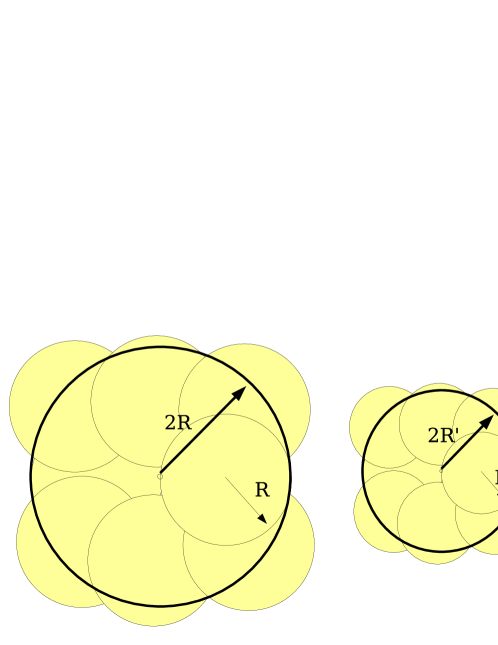
Figure 1: The metric space defined by a set of points in $\mathbb{R}^{2}$ and the Euclidean distance is doubling. Indeed, we can cover a disc of radius $2R$ by a constant ($8$ in this case) number of discs of radius $R$, whatever the value of $R$.

In Section II-A, we describe the geometric random graph model, which will be the canonical model we will use to illustrate the ideas of the paper. We also give an example of a non-homogeneous network to which our results can be applied. In Section II-B, we will develop the model where connectivity is determined by the SINR, and we have uniform transmit power and full connectivity. We give the requirements for the mobility model to result in a smooth sequence of wireless network graphs in Section II-C. We state the underlying assumptions and give a table of notations in Section II-D.

II-A Geometric random graph

We denote the geometric random graph by $\mathcal{G}(n,r_{n})$ and define its connectivity as follows.

Definition 4

A random geometric graph $\mathcal{G}(n,r_{n})$ has an unweighted edge between nodes $u$ and $v$ if and only if $||x(u)-x(v)||<r_{n}$, where $\{x(u)\}$ are chosen independently and uniformly in $\left[0,\sqrt{n})\right.\times\left[0,\sqrt{n})\right.$.

In this paper we will be interested in fully connected geometric random graphs, and therefore focus on the case $r_{n}>\sqrt{\log n}$ [GK98]. As a natural extension, we can also define a sequence of random graphs $\mathcal{G}^{(t)}(n,r_{n})$ with an unweighted edges between $u$ and $v$ at time $t$ if $||x^{(t)}(u)-x^{(t)}(v)||<r_{n}$. Whether each graph in the sequence $\mathcal{G}^{(t)}(n,r_{n})$ corresponds to a random geometric graph as in Definition 4, depends on the mobility model for the nodes. We discuss this in more detail in Section II-C.

In Figure 2, we illustrate a non-homogeneous random network where connectivity is not completely geometric as in Definition 4. An obstacle prevents communication between neighboring nodes, and therefore illustrates the complexities of wireless network connectivity. This example is revisited in Section III, where we show that though this connectivity graph is more complicated than $\mathcal{G}(n,r_{n})$, it is still doubling, and therefore the algorithms developed in this paper are applicable. This illustrates the advantage of our approach to network modeling.

Figure 2: $n$ nodes are distributed uniformly at random on a square area of side $\sqrt{n}$. A wall of width $r_{n}/c$ is added, which only has a small hole in the middle. Again, we assume $r_{n}>\sqrt{\log n}$. Nodes cannot communicate through the wall. Finally, we remove the nodes below the wall, which leads to an inhomogeneous node distribution.

II-B SINR full connectivity

Since the wireless channel is a shared medium, the transmissions between nodes interfere with each other. However, the signal strength decays as a function of the distance traveled, and therefore we can define the SINR for transmission from node $u$ to $v$ as,

$$\mathrm{SINR}=\frac{P_{n}||x(u)-x(v)||^{-\beta}}{N_{0}+\sum_{w\neq u,v}P||x(w)-x(v)||^{-\beta}},$$ (1)

where $\beta$ is a distance loss (decay) parameter depending on the propagation environment, $P_{n}$ is the common transmit power of the nodes and $N_{0}$ is the noise power. We can of course easily adapt this to have power control for the nodes. A transmission is successful if the SINR is above some constant threshold value $\varsigma$. For static nodes, just as in the case of geometric random graph, we assume that the node locations $\{x(u)\}$ are chosen independently and uniformly in $\left[0,\sqrt{n})\right.\times\left[0,\sqrt{n})\right.$. This model for wireless networks has been extensively studied in the literature (see [GK00, KV02]). The authors base their analysis of the capacity of wireless networks on a TDMA scheme for the SINR connectivity model of (1). We argue here that the structure of the resulting connectivity graph is identical to that of $\mathcal{G}(n,r_{n})$, for $r_{n}>\sqrt{\log n}$. Therefore, the results we prove for $\mathcal{G}(n,r_{n})$, would also be applicable to such graphs. In practice, it is a non-trivial task to design a distributed scheduling protocol (MAC layer protocol) that mimics the behavior of this TDMA scheduler. However, these MAC layer implementation issues are far beyond the scope of this document (see for instance [MSZ06]). We only make the argument here that the connectivity graph resulting from such a TDMA scheme would yield the same behavior as a $\mathcal{G}(n,r_{n})$.

We will subdivide the network into small squares of side $s_{n}=\frac{r_{n}}{c}$. We need to show that if two nodes $u$ and $v$ are in neighboring small squares (and so have the guarantee that they can communicate under the $\mathcal{G}(n,r_{n})$ model as we will see in the sequel), then there exists a TDMA scheme that allows them to communicate under the SINR connectivity model of (1). If this is the case, then we can apply the same proof techniques for both models. We let the maximum transmission power grow in the same way as we did for the $\mathcal{G}(n,r_{n})$ model i.e. $P_{n}\leq(N_{o}\varsigma r_{n})^{\beta}$. Additionally, we want to design a TDMA scheme such that the capacity of all links is at least $O(\frac{1}{\log n})$ $\left[bits/sec\right]$. It can be shown (see [RS98]) that every small square contains at most $O(\log n)$ nodes. Hence, we ask that the traffic can flow at constant rate independent of $n$ between neighboring small squares, and that each node is treated equally. Note that this requirement is very similar to the scheme proposed in [GK00] in which one node per small square can transmit at constant rate to any neighboring square.

Theorem 1

There exists a TDMA scheme such that all nodes can communicate with any node located in a neighboring small square at a rate of $O(\frac{1}{\log(n)})$ $\left[bits/sec\right]$. Hence, the aggregate traffic can flow between neighboring small squares at a constant rate independent of $n$.

Proof:

We take a coordinate system, and label each square with two integer coordinates. Then we take an integer $k$, and consider the subset of squares whose two coordinates are a multiple of $k$ (see Figure 3). By translation, we can construct $k^{2}$ disjoint equivalent subsets. This allows us to build the following TDMA scheme: we define $k^{2}$ time slots, during which all nodes from a particular subset are allowed to transmit for the same duration of $O(\frac{1}{\log n})$ seconds. Each small square contains at least one and at most $O(\log n)$ nodes w.h.p. (see [RS98] and the proof of Theorem 3). We assume also that at most one node per square transmits at the same time, and that they all transmit with the same power $P_{n}$.

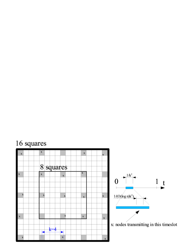
Figure 3: Illustration of the TDMA scheduling scheme.

Let us consider one particular square. We suppose that the transmitter in this square transmits towards a destination located in a square at distance at most $1$. We compute the signal-to-interference ratio at the receiver. First, we choose the number of time slots $k^{2}$ as follows: $k=4$. To find an upper bound to the interferences, we observe that with this choice, the transmitters in the $8$ first closest squares are located at a distance at least $3$ (in small squares) from the receiver (see left-hand side of Figure 3). This means that the Euclidean distance between the receiver and the $8$ closest interferers is at least $2s_{n}$. The $16$ next closest squares are at distance at least $7$ (in small squares), and the Euclidean distance between the receiver and the $16$ next interferers is therefore at least $6s_{n}$, and so on. The sum of the interferences $I$ can be bounded as follows:

$$\begin{array}[]{ll}I&\leq\sum_{i=1}^{\infty}8iP_{n}\left[2s_{n}(2i-1)\right]^{-\beta}\\ &=P_{n}\left[2s_{n}\right]^{-\beta}\sum_{i=1}^{\infty}8i\left[(2i-1)\right]^{-\beta}\\ &=(N_{o}\varsigma r_{n})^{\beta}\left[2\frac{r_{n}}{c}\right]^{-\beta}\sum_{i=1}^{\infty}8i\left[(2i-1)\right]^{-\beta}\end{array}$$

This term clearly converges if $\beta>2$. Now we want to bound from below the strength of the signal received from the transmitter. We observe first that the distance between the transmitter and the receiver is at most $\sqrt{2(s_{n}^{2})}\leq 2s_{n}$. The strength $S$ of the signal at the receiver can thus be bounded by

$$\begin{array}[]{ll}S&\geq P_{n}\min\left\{1,2s_{n}^{-\beta}\right\}\\ &=O(1)\end{array}$$

Finally, we obtain the following bound on the SINR: $SINR\geq\frac{S}{N_{o}+I}$. As the above expression does not depend on $n$, the theorem is proven. ∎

II-C Uniform speed-limited (USL) mobility

Nodes are mobile and move according to the uniform speed-limited (USL) model, a fairly general mobility model defined next. The USL model essentially embodies two conditions: (i) the node distribution at every time step is uniform over the network domain, and (ii) the distance a node can travel over a time step is bounded. We restrict ourselves to the case in which the maximum speed is not dependent on $n$. In practice, of course, such an assumption is realistic since the maximum speed of the nodes will not increase when new nodes join the network.

Definition 5

A collection of $n$ nodes satisfy the uniform speed-limited (USL) mobility model if the following two conditions are satisfied:

1. At every time $t$, the distribution of nodes over the network domain is uniform;

2. For every node $u$ and time $t$, the distance traveled in the next time step is bounded, i.e., $||x^{(t+1)}(u)-x^{(t)}(u)||<S$.

The USL mobility model is quite general. For example, it includes the following cases: (i) The nodes perform independent random walks with bounded one-step displacement. The random walks can be biased, and the displacement distribution does not need to be homogeneous over the node population. We have to assume that the nodes operate in the stationary regime. (ii) The nodes follow the random waypoint model (RWP). The system has to be in the stationary regime. (iii) The generalized random direction models from [SMS06], which interpolate between the random walk and the random waypoint cases, through a control parameter that can be viewed as the ”locality” of the mobility process. (iv) We can also allow for models where nodes do not move independently. As an illustrative example, assume we uniformly place nodes on the square; the nodes then move in lockstep according to any speed-limited mobility process, maintaining their relative positions to each other. Observe that the uniform distribution is maintained for all time steps (note that we move on a torus), and that the speed-limited property is true by definition.

We see that the USL class of mobility models is fairly general, and includes many of the models that have been proposed in the literature. For simplicity, we consider that time is discrete. In other words, we look at a snapshot of the network every $\Delta T$ seconds. At every time step, the connectivity between nodes will be modified. Hence, we will work with a sequence of connectivity graphs. In order to design a routing algorithm with a low control traffic overhead, we will need to understand how fast the graph distances between nodes can evolve over time. In particular, consider two nodes $u$ and $v$ at distance $d=d^{t}(u,v)$ at time $t$. We want to bound the multiplicative factor by which this distance can change in $\kappa$ time steps. Formally, we define $\kappa(\tau,d)$ as follows:

Definition 6

We say that a communication network is $\kappa(\tau,d)$-smooth if the shortest path distance between any two nodes $u$ an $v$ at shortest path distance $d$ cannot change by more than a factor $\kappa(\tau,d)$ in $\tau$ time steps i.e., $\forall u,v$, we have:

$$\max\left\{\frac{d^{(t)}(u,v)}{d^{(t+\tau)}(u,v)},\frac{d^{(t+\tau)}(u,v)}{d^{(t)}(u,v)}\right\}\leq\kappa(\tau,d)$$

Additionally, we simply say that the network is $\kappa$-smooth if there exists a constant $\nu$ such that $\kappa(\nu d,d)\leq\kappa(\nu)=\kappa$ independently of $d$. In this case, the distances grow at the same speed at all scales. In the sequel, we will bound $\kappa$ and $\nu$ for our model. This USL property holds for a general class of random trip mobility models studied in [BV05], where it is shown that the stationary distribution of such mobility models is uniform and ergodic. We restate this theorem without proof.

Theorem 2

([BV05]) The random-trip mobility model has uniform stationary distribution on $[0,a)\times[0,a)$.

II-D Assumptions

We consider that a time step $\Delta T$ is much larger than the round trip time (RTT) through the network i.e., the time scale for mobility is much larger than the time scale for communications. For clarity and in order to simplify the analysis, we will make the assumption that nodes can communicate instantaneously through the network. We also make the assumption that there is a random permutation $\pi$ on the nodes, and that all nodes in the network know their rank in the permutation. In Section VI we will then drop these assumptions and consider practical aspects of the implementation. Finally, we say that a result holds with high probability (w.h.p.) if it holds with probability at least $(1-O(\frac{1}{n^{\rho}}))$, for some constant $\rho>0$. In Table I, we summarize the notations used in this paper.

$x^{(t)}(u)$	Position of node $u$ at time $t$
$d^{(t)}(u,v)$	Shortest path distance from $u$ to $v$ at time $t$
$r_{n}$	Wireless communication radius
$\mathcal{G}(n,r_{n})$	Random geometric graph
$\mathcal{B}_{R}^{(t)}(u)$	Ball of radius $R$ around $u$
$\kappa(\tau,d)$	$\max\left\{\frac{d^{(t)}(u,v)}{d^{(t+\tau)}(u,v)},\frac{d^{(t+\tau)}(u,v)}{d^{(t)}(u,v)}\right\}\leq\kappa(\tau,d)$

TABLE I: Table of notations

III Network Properties

In this section, we prove some properties of the network models presented in Section II, which are necessary to analyze the performance of our algorithm. We focus our attention on the geometric random graph $\mathcal{G}(n,r_{n})$, but all the arguments can be extended to the SINR full connectivity model with TDMA scheduling, discussed in Section II-B. In particular, for $\mathcal{G}(n,r_{n})$, we now consider the case in which the communication radius $r_{n}$ is such that $r_{n}=\sqrt{(1+\epsilon)\log{n}}>\log^{1/2}n$, where $\epsilon>0$.

For uniform speed-limited (USL) mobility models discussed in Section II-C, at each time, the node locations $\{x^{(t)}(u)\}$ have a distribution that is uniform over $\left[0,\sqrt{n})\right.\times\left[0,\sqrt{n})\right.$. Therefore, we now discuss the property of a sequence of geometric random graphs, $\mathcal{G}^{(t)}(n,r_{n})$, under USL mobility model. We subdivide the network area on which the nodes live into smaller squares of side $\frac{r_{n}}{c}$, where $c$ is a constant chosen such that nodes in neighboring squares are connected (see Fig. 4) and that an integer number of squares fit into the network area.

Figure 4: Nodes in neighboring squares are connected

We arbitrarily set $c=\sqrt{5}$. We number the small squares from $1$ to $m=\frac{n}{(r_{n}/c)^{2}}=\frac{nc^{2}}{(1+\epsilon)\log{n}}$ and denote by $E_{i}$ the event that small square $i$ does not contain any node, in a sequence of length $n^{\rho}$ time steps, for some constant $\rho$. In the next theorem, we show that when nodes move according to USL mobility model, all small squares will be populated w.h.p.

Theorem 3

There exists a constant $\rho$ such that if we divide the network into small square of side $\frac{r_{n}}{c}$ (with $r_{n}>\sqrt{\log{n}}$), at every time step in a sequence of length $n^{\rho}$, every small square contains at least one node w.h.p.

Proof:

Consider a sequence of length $Z=n^{\rho}$. Denote by $E_{i}^{(j)}$ the event the small square $i$ is empty at time $j$. Let $m=\frac{n}{r_{n}^{2}}$. We can compute:

$$\begin{array}[]{ll}\mbox{$\mathcal{P}\left[\bigcup_{j=1}^{Z}\bigcup_{i=1}^{m}E_{i}^{(j)}\right]$}&\leq Z\sum_{i=1}^{m}\mbox{$\mathcal{P}\left[E_{i}^{(j)}\right]$}\\ &=Z\sum_{i=1}^{m}(1-\frac{1}{m})^{n}\\ &\leq Z\sum_{i=1}^{m}e^{-\frac{n}{m}}\\ &=Z\frac{nc^{2}}{(1+\epsilon)\log{n}}e^{-\frac{nc^{2}(1+\epsilon)\log{n}}{n}}\\ &\leq Z\frac{nc^{2}}{(1+\epsilon)\log{n}}\frac{1}{n^{(1+\epsilon)}}\\ &=Z\frac{c^{2}}{(1+\epsilon)n^{\epsilon}\log{n}}\\ &\leq O(\frac{n^{\rho}}{n^{\epsilon}})\\ &=O(\frac{1}{n^{\epsilon-\rho}})\end{array}$$

We can now choose $\rho$ such that $\epsilon-\rho>0$ and the result follows. ∎

It is immediate that a in single instantiation of the connectivity graph (i.e., time step), every small square is populated w.h.p.

Corollary 1

With probability at least $(1-O(\frac{1}{n^{\epsilon}}))$, there is no empty small square in a sequence of length $1$.

We are now ready to show that at every time step in a sequence of $n^{\rho}$ connectivity graphs, the connectivity graph is doubling w.h.p. Since we have a USL mobility model, any graph $\mathcal{G}^{(t)}(n,r_{n})$ is statistically identical to $\mathcal{G}(n,r_{n})$.

Theorem 4

$\mathcal{G}(n,\sqrt{(1+\epsilon)\log{n}})$ are doubling w.h.p.

Proof:

By Lemma 1, all small squares contain at least one node w.h.p. Consequently, neighboring squares (vertically and horizontally) have at least one communication link. Denote by $\mathcal{L}(m,r)$ the grid having the small squares as vertices, and with edges between vertical and horizontal neighbors. Consider a ball $B_{upper}=\mbox{$\mathcal{B}_{2R}^{\mathcal{G}}(u)$}$ centered around some node $u$. Clearly, all nodes in $B_{upper}$ must be contained in a square which is part of $\mathcal{B}_{4Rc}^{\mathcal{L}}(u)$ i.e., $B_{upper}\subseteq\mbox{$\mathcal{B}_{4Rc}^{\mathcal{L}}(u)$}$. This follows from the fact that no node in $B_{upper}$ can be further away from $u$ than $2Rr$ in Euclidean distance, and that the grid is fully connected w.h.p. Similarly, one can see that $\mbox{$\mathcal{B}_{R}^{\mathcal{L}}(u)$}\subseteq B_{lower}=\mbox{$\mathcal{B}_{R}^{\mathcal{G}}(u)$}$. This is a consequence of the fact that $\mathcal{L}$ is a subgraph of $\mathcal{G}$, i.e., two nodes in small squares $R$ hops a part in $\mathcal{L}$ cannot be more than $R$ hops apart in $\mathcal{G}$ (see Fig. 5). For an appropriately chosen constant $\alpha$, we have:

$$B_{upper}\subseteq\mbox{$\mathcal{B}_{4Rc}^{\mathcal{L}}(u)$}\subseteq\bigcup_{j=1}^{\alpha}\mbox{$\mathcal{B}_{R}^{\mathcal{L}}(v_{j})$}\subseteq\bigcup_{j=1}^{\alpha}\mbox{$\mathcal{B}_{R}^{\mathcal{G}}(v_{j})$}$$ (2)

and $\mathcal{G}(n,\sqrt{(1+\epsilon)\log{n}})$ is doubling.

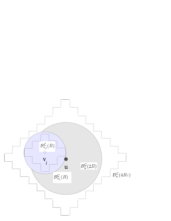
Figure 5: Proof of theorem 4

∎

Note that it is possible to build a deterministic geometric graph for which this property does not hold (see Appendix Unit Disc Graphs). Further, one can show that $\mathcal{G}(n,r_{n})$ are not doubling w.h.p when $r_{n}<\sqrt{\log n}$. We prove this result in Appendix Random Geometric Graphs with $r_{n}<\sqrt{\log n}$. At this point, we would like to emphasize that even though we analyze networks in which the nodes are uniformly distributed on a square area, the doubling property is a much more powerful tool. Indeed, our results and algorithms depend only on the doubling constant. Consequently, the algorithms and the bounds can be applied to any other type of networks or node configuration which lead to a doubling connectivity graph. For instance, one can consider the network shown in Figure 2, described in Section II-A. It can easily be shown by using a technique similar to the one used in Theorem 4 that this network is doubling. While we can seamlessly apply our routing algorithm to such a network, any classical geographic routing algorithm would fail or require a high control traffic overhead to get out of dead-ends. This is because nodes would get stuck against the wall when routing packets from the lower to the upper part of the network. In turn, this would considerably degrade the performance in terms of stretch and control traffic overhead with respect to the same network without a wall. In the next subsection we prove a set of sufficient conditions for a wireless networks to have a constant doubling dimension.

III-A Inhomogeneous Topologies

In the first part of this subsection, we show that under certain conditions, the presence of topological holes (obstacles) in the network does not increase the doubling property, or only by a constant factor. In particular, we are interested in how we can alter the topology of a fully connected and dense network by removing nodes while still preserving the doubling property. In the second part, we will generalize this idea to arbitrary metric spaces. Consider a $\mathcal{G}(n,r_{n})$ with $r_{n}>\sqrt{\log n}$, such that full connectivity is guaranteed. The network area is divided into squarelets of side $\frac{r_{n}}{c}$, where $c$ is chosen such that nodes in horizontally and vertically adjacent squarelets are guaranteed to be within communication range. We now arbitrarily select squarelets and remove all nodes they contain. We denote the new graph we obtain by $\mathcal{G}_{n}$ .

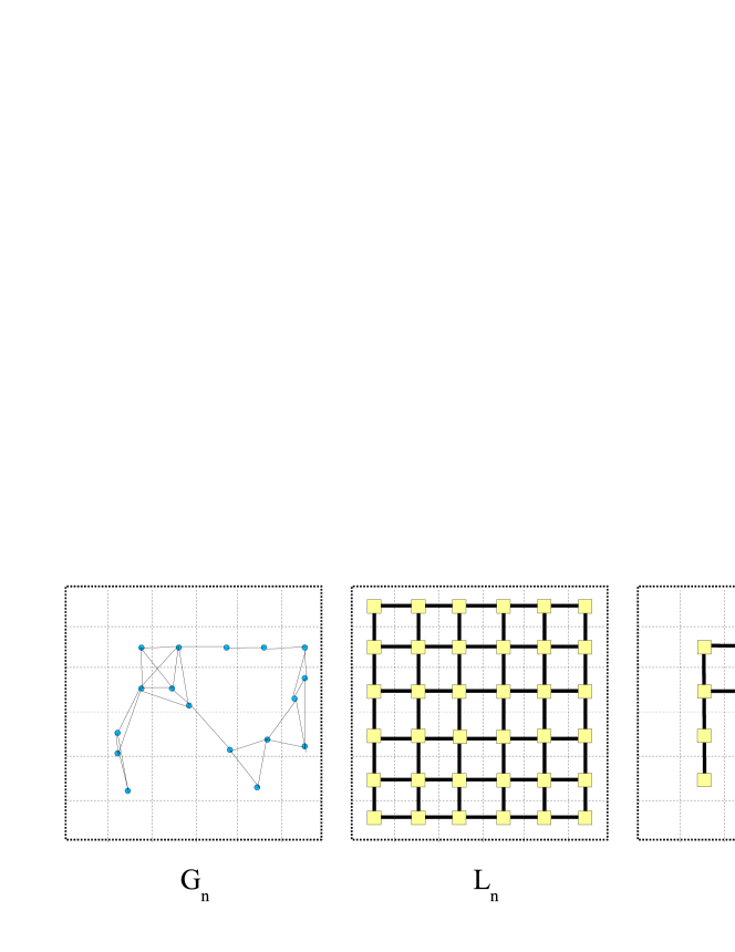
Figure 6: Graphs $\mathcal{G}_{n}$ , $\mathcal{L}_{n}$ and $\mathcal{H}_{n}$ . The network area is divided into squarelets of side $\frac{r_{n}}{c}$ such that nodes in horizontally and vertically adjacent squarelets are guaranteed to be within communication range.

We denote by $\mathcal{L}_{n}$ the full grid where the squareletes are vertices and by $\mathcal{H}_{n}$ the corresponding grid in $\mathcal{G}_{n}$ i.e., the thinned out grid obtained by selecting only non-empty squarelets in $\mathcal{G}_{n}$ . In $\mathcal{L}_{n}$ , we add an edge between horizontally and vertically adjacent squarelets (see Fig. 6). In $\mathcal{H}_{n}$ , we first add a an edge between horizontally and vertically squarelets containing at least one node. Then, for every pair of squarelets containing nodes that can communicate directly, we add an edge of weight corresponding to the distance between those two squarelets in $\mathcal{L}_{n}$ . We add the edges from the shortest to the longest one, and only if no path of the same length already exists in $\mathcal{H}_{n}$ . We can now define a topological hole as follows:

Definition 7 (Topological Hole)

A set of horizontally, vertically and horizontally adjacent empty squarelets in the graph $\mathcal{H}_{n}$ is called a hole if adding a (virtual) vertex in all of the squarlets in that set modifies the distance between at least two vertices in $\mathcal{H}_{n}$ .

Let us denote by $\mathcal{V}_{k}$ the $k^{th}$ hole (k=1,2,3,…). We define the perimeter $p(\mbox{$\mathcal{V}_{k}$})$ of $\mathcal{V}_{k}$ as 2 times the maximum distance between any two vertices on the border of the hole i.e, in squarelets adjacent to the empty squarelets defining the hole. Note that for all $u,v$, we have $d^{\mbox{$\mathcal{H}_{n}$ }}(s_{u},s_{v})\geq d^{\mbox{$\mathcal{G}_{n}$ }}(u,v)$.

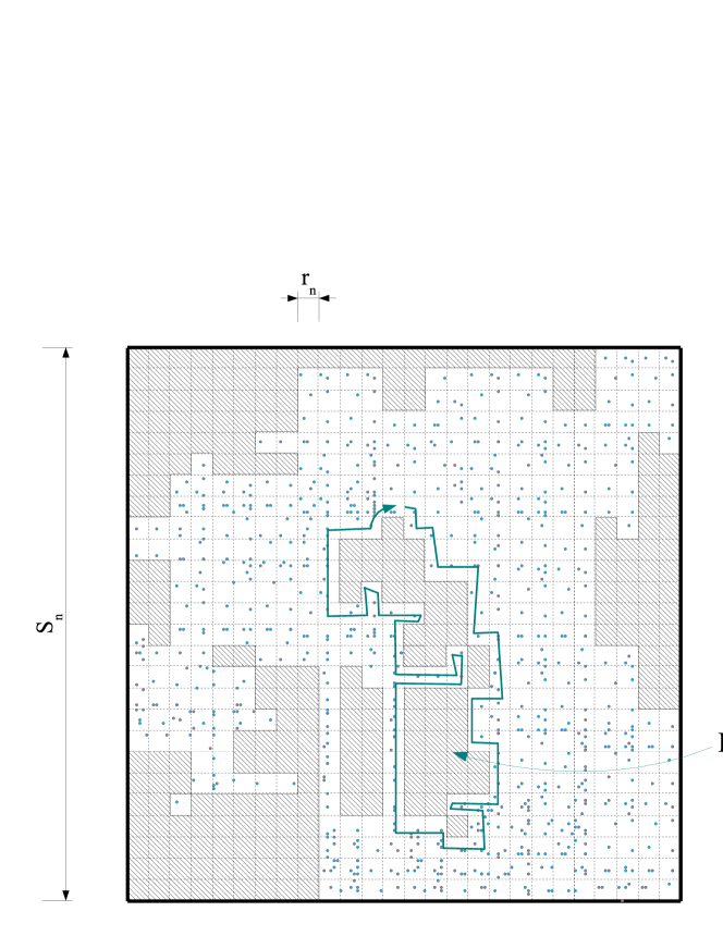
Figure 7: A network with holes

Theorem 5

Let $P=\max_{k}p(\mbox{$\mathcal{V}_{k}$})$. Then, the doubling dimension is upper bounded by $O(P^{2})$.

Proof:

Consider a ball $\mathcal{B}_{2R}^{\mbox{$\mathcal{G}_{n}$ }}(u)$ centered at $u$ in $\mathcal{G}_{n}$ . First, observe that $\mbox{$\mathcal{B}_{2R}^{\mbox{$\mathcal{G}_{n}$ }}(u)$}\subseteq\mbox{$Box_{2Rc}^{\mbox{$\mathcal{L}_{n}$ }}(u)$}$, where $Box_{2Rc}^{\mbox{$\mathcal{L}_{n}$ }}(u)$ is the box centered at the squarelet containing $u$ in $\mathcal{L}_{n}$ which contains all nodes at “maximum norm” $2Rc$ (i.e., $l_{\infty}$-norm) from this squarelet. In other words, all nodes within $2R$ hops from $u$ in $\mathcal{G}_{n}$ must be in a squarelet contained in this box. We will now cover this box with smaller boxes $Box_{\max\left\{1,\left\lceil\frac{R}{4\gamma}\right\}\right\rceil}^{\mbox{$\mathcal{L}_{n}$ }}(s_{v_{i}})$. We need $\left\lceil\frac{16R^{2}c^{2}4\gamma^{2}}{R^{2}}\right\rceil=64c^{2}\gamma^{2}$ such boxes at most. Consider the same small boxes in $\mathcal{H}_{n}$ . Pick one non-empty squarelet $s_{v_{i}}$ in each such small boxes. Note that the maximum hop distances between two squarelets in such a small box in $\mathcal{L}_{n}$ is at most $\frac{R}{\gamma}$. For each of these hops, we might have to make a detour of at most $P$ steps. Consequently, the same two squarelets could be at distance at most $\frac{PR}{\gamma}$ in $\mathcal{H}_{n}$ . Observe now that for any two nodes $u$ and $w$ contained in squarelets $s_{u}$ and $s_{w}$ respectively, we have $d^{\mbox{$\mathcal{H}_{n}$ }}(s_{u},s_{w})\geq d^{\mbox{$\mathcal{G}_{n}$ }}(u,w)$. For each squarelet $s_{v_{i}}$, we pick one node $v_{i}$ contained in this squarelet. Hence, for all nodes $w$ contained in this small box, we have $d^{\mbox{$\mathcal{G}_{n}$ }}(v_{i},w)\leq d^{\mbox{$\mathcal{H}_{n}$ }}(s_{v_{i}},s_{w})\leq\frac{PR}{\gamma}$. By setting $\gamma=P$, we obtain the claim. ∎

We can extend this result to the case where the network can be divided into convex sets. We define a convex set in $\mathcal{G}_{n}$ with slack as follows:

Definition 8

Let $\Psi$ be a set of nodes in $\mathcal{G}_{n}$ . Let $\mbox{$\mathcal{H}_{n}$ }^{(\Psi)}$ be the squarelets in $\mathcal{H}_{n}$ containing at least one node in $\Psi$. We say that the set $\Psi$ is convex if $\forall u,v\in\Psi$, $d^{\mbox{$\mathcal{H}_{n}$ }^{(\Psi)}}(s_{u},s_{v})=d^{\mbox{$\mathcal{L}_{n}$ }}(s_{u},s_{v})$, where $s_{u}$ and $s_{v}$ are the squarelets containing $u$ and $v$ i.e., there must be at least one shortest path inside the convex set. We say that the set $\Psi$ is convex with slack P if $d^{\mbox{$\mathcal{H}_{n}$ }^{(\Psi)}}(s_{u},s_{v})\leq Pd^{\mbox{$\mathcal{L}_{n}$ }}(s_{u},s_{v})$.

We can now state the following theorem

Theorem 6

Let $\zeta_{1},\zeta_{2},...,\zeta_{q}$ be a partition of the network into $q$ convex sets with slack $P_{1},P_{2},...,P_{q}$ respectively. Let $per_{1},per_{2},...,per_{q}$ denote the perimeter of the convex sets. The doubling dimension is then upper bounded by $\max_{u,\rho}4\sum_{\zeta_{i}:\zeta_{i}\cap\mbox{$Box_{\rho}^{\mbox{$\mathcal{L}_{n}$ }}(s_{u})$}\neq\emptyset}(\left\lceil\frac{per_{i}}{\frac{\rho}{P_{i}}}\right\rceil)^{2}$.

Proof:

In the proof of Theorem 5, we have shown that any ball of radius $2R$ around some node $u$ is contained in a box $Box_{\rho}^{\mbox{$\mathcal{L}_{n}$ }}(s_{u})$, where $\rho=2Rc$. We can cover each convex set $\zeta_{i}$ intersecting this box with at most $4(\left\lceil\frac{per_{i}}{\frac{\rho}{P_{i}}}\right\rceil)^{2}$ small boxes of radius $R/4P_{i}$, as shown in Theorem 5. A slack of $P$ implies that by selecting one node in each of the small boxes, all nodes in the convex set are within $R$ hops of this node in $\mathcal{G}_{n}$ . If the box $Box_{\rho}^{\mbox{$\mathcal{L}_{n}$ }}(s_{u})$ is partitioned into several convex sets, selecting $4(\left\lceil\frac{per_{i}}{\frac{\rho}{P_{i}}}\right\rceil)^{2}$ nodes in each convex set $\zeta_{i}$ intersecting this box will in turn guarantee that all nodes are covered. ∎

In practice, this result implies that if we are given a decomposition of the network into convex sets, we can bound the overall doubling dimension given the doubling dimension of each set separately. Further, this result implies that networks that consist of a small number of convex areas, which can each contain arbitrarily many small holes, have a low complexity in terms of doubling dimension. We will now relate the “shapes” of a topological hole to the doubling dimension. In particular, we will show that one can relate the doubling dimension to the maximum number of connected components in any square subarea.

Theorem 7

For any $\gamma\geq 2$, the doubling dimension $\alpha$ is such that

$$\alpha\leq 4\gamma^{2}c^{2}\max_{\mbox{$Box_{R/\gamma}^{\mbox{$\mathcal{L}_{n}$ }}(u)$}}\left\{\mbox{number of convex disconnected components with slack $\gamma$ in \mbox{$Box_{R/\gamma}^{\mbox{$\mathcal{L}_{n}$ }}(u)$}}\right\}$$

Proof:

In the proof of Theorem 5, we have shown that any ball of radius $2R$ around some node $u$ is contained in a box $Box_{\rho}^{\mbox{$\mathcal{L}_{n}$ }}(s_{u})$, where $\rho=2Rc$. In turn, we showed that by dividing this box into smaller boxes of side $R/\gamma$, and by selecting one node in each box, we could cover the larger ball of radius $2R$. Now, in each small box of side $R/\gamma$, the presence of holes might create several disconnected components. However, we know that inside each such component, we can cover any convex subset with slack $\gamma$ with one nodes. The result follows. ∎

This last result gives us a characterization of the alterations we can make to a fully connected $\mathcal{G}(n,r_{n})$ network, while only affecting the doubling dimension by a constant factor. In particular, we can remove nodes as long as we do not create too many convex and disconnected components in any square subarea. Note that we can still remove arbitrarily many nodes as long as we only create small holes. Theorems 5, 5, 5 imply that topologies such as the one shown in Fig. 8 have a constant doubling dimension.

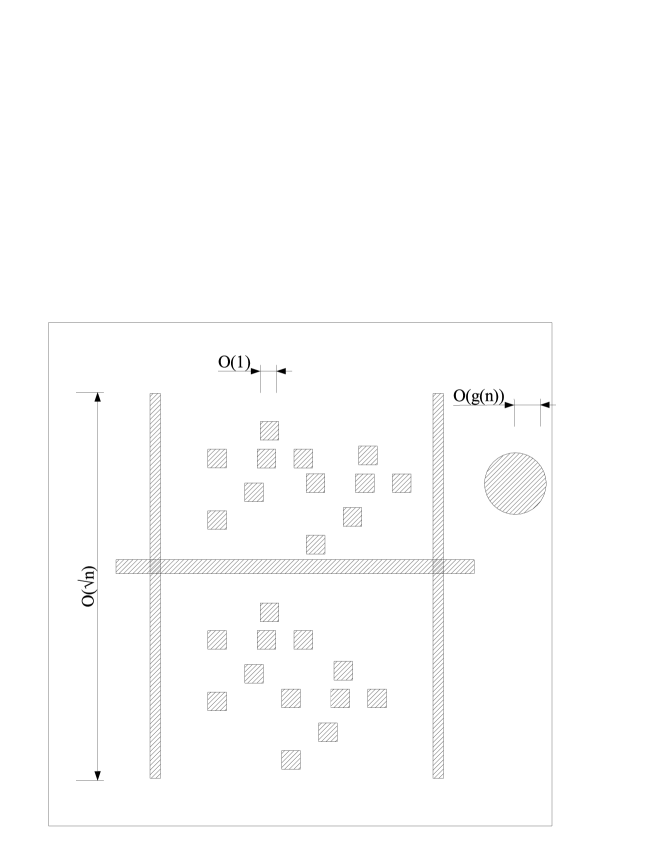
Figure 8: A network with topological holes and a constant doubling dimension. The size of the large holes grow with $n$, but the network can be divided into a constant number of areas, each being convex with slack $O(1)$ i.e., each of the convex areas contains only obstacles with a constant perimeter or that can only increase the distance between nodes by a constant factor. Note that even though the doubling dimension is low, greedy geographic forwarding of packets would fail as packets would get stuck in dead-ends against the holes. Squarelets containing no nodes are hatched.

The results stated above are special cases of the more general result detailed in the sequel. Indeed, we can relate the doubling dimension in a metric space to the doubling dimension in another metric space if we know the distortion of the embedding that maps the points in one metric space to the points in the other metric space. The example above is a special case of that setup where we map the nodes of a graph to points in Euclidean space. Consider two metric spaces $(X,d)$ and $(X^{\prime},d^{\prime})$, where $d$ and $d^{\prime}$ are distance functions which define a metric on the sets of point $X$ and $X^{\prime}$. We could for instance consider the two metric spaces $(\mathcal{X},||.||)$ and $(\mathcal{H},d(.,.))$ i.e., the points in the plane with the Euclidean distance and the nodes in the graph with the shortest path distance. A metric embedding is a bijective function $\phi:\mathcal{X}\rightarrow\mathcal{X^{\prime}}$ which associates to a point in one metric space a point in another metric space.

Definition 9 (Distortion of an Embedding)

A mapping $\phi:X\rightarrow X^{\prime}$ where $(X,d)$ and $(X,d^{\prime})$ are metric spaces, is said to have distortion at most $D$, or to be a D-embedding, where $D\geq 1$, if there is a $K\in(0,\infty)$ such that $\forall x,y\in X$,

$$Kd(x,y)\leq d^{\prime}(\phi(x),\phi(y))\leq KDd(x,y)$$

if $X^{\prime}$ is a normed space, we typically require $K=1$ or $K=\frac{1}{D}$. An embedding has distortion $D$ with slack $\epsilon$ if all but an $\epsilon$ fraction of node pairs have distortion $D$ under $\phi$. Additionally, one can loosen this definition by allowing slack. The slack is said to be uniform if each node has distortion at most $D$ to a $1-\epsilon$ fraction of the other nodes. Finally, an embedding with distortion $D$ and slack $\epsilon$ is coarse if for every node $u$ the distortion is bounded to a node a distance greater than $r_{\epsilon}=inf\left\{r\mbox{s.t }|\mbox{$\mathcal{B}_{r}^{X}(u)$}|>\epsilon n\right\}$.

The doubling dimension of a metric space embedded into another metric space can be bounded as follows:

Theorem 8 (Bounding the Doubling Dimension)

Consider a metric space $(\mathcal{H},d)$ embedded in another metric space $(\mathcal{E},d^{\prime})$ by a function $\phi$. Let the doubling dimension of $\mathcal{E}$ be $\beta$. Let the distortion of this embedding be $D$. Then, $\mathcal{H}$ has doubling dimension $\alpha$ with $\alpha\leq O((2D)^{\log\beta})$.

Proof:

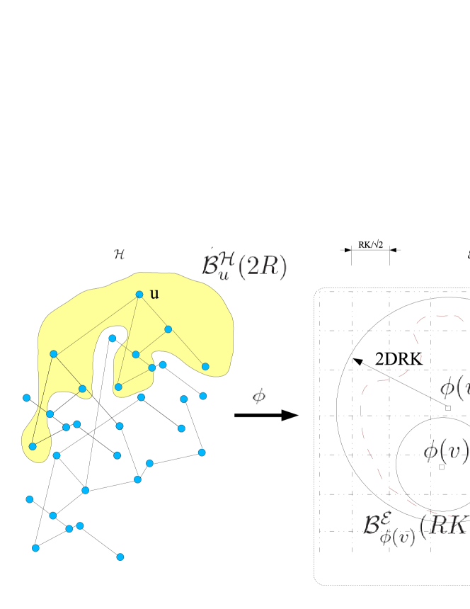
Figure 9: Proof of Theorem 8

Choose any node $u\in\mathcal{H}$. If the above condition is fulfilled, the images of all nodes in $\mathcal{B}_{2R}^{\mathcal{H}}(u)$ can be at distance $d^{\prime}$ at most $2KDR$ from $u$ at $\phi(u)$. Hence, $\phi(\mbox{$\mathcal{B}_{2R}^{\mathcal{H}}(u)$})\subset\mbox{$\mathcal{B}_{2KDR}^{\mathcal{E}}(\phi(u))$}$. We will now try to cover $\phi(\mbox{$\mathcal{B}_{2R}^{\mathcal{H}}(u)$})$ by as few balls $\mathcal{B}_{RK}^{\mathcal{\mathcal{E}}}(\phi(v))$ as possible (see Fig. 9, which illustrates this setup in the case when $\mathcal{H}$ is a graph and $\mathcal{E}$ the Euclidean space). To do so, let us cover $\mathcal{B}_{2KDR}^{\mathcal{E}}(\phi(u))$ by small balls of radius $KR$ in $\mathcal{E}$. Covering $\mathcal{B}_{2KDR}^{\mathcal{E}}(\phi(u))$ will require at most $\beta^{\log 2D}$ balls of radius $KR$ in $\mathcal{E}$, given that $\mathcal{E}$ has doubling dimension $\beta$. We know that $d(u,v)\leq d^{\prime}(u,v)/K$, by definition 9. Consequently, $\phi^{-1}(\mbox{$\mathcal{B}_{RK}^{\mathcal{\mathcal{E}}}(\phi(v))$})\subset\mbox{$\mathcal{B}_{R}^{\mathcal{H}}(v)$}$. We can conclude that $\mbox{$\mathcal{B}_{2R}^{\mathcal{H}}(u)$}\subset\bigcup_{j=1}^{\beta^{\log 2D}}\mbox{$\mathcal{B}_{R}^{\mathcal{H}}(v_{j})$}$. ∎

The presence of large obstacles in the network does not necessarily imply that the network is not doubling. In particular,

Theorem 9

Consider a metric space $\mathcal{E}$ with doubling dimension $\beta$. A metric space $\mathcal{H}$ that can be divided in $k$ sets $S_{1},S_{2},...,S_{k}$, such that each set embeds individually with distortion $D_{i}$ into $\mathcal{E}$ has doubling dimension at most $\sum_{j=1}^{k}\beta^{2\log 2D_{j}}$.

Proof:

Consider any ball of radius $2R$ in $\mathcal{H}$, such that the nodes in the ball belong to at least two different sets (otherwise the theorem is clearly true). Note that the radius of each of these subsets can be at most $4R$. Consequently, we now that the part of the ball that belongs to $S_{i}$ can be covered by at most $\beta^{2\log 2D_{i}}$ (by applying Theorem 8 to cover a ball of radius $4R$ by balls of radius $R$). The theorem follows. ∎

We can now broaden the class of communication networks that have low doubling dimension. In particular, if we can subdivide the communication graph into a constant number of subsets, such that each one embeds with constant distortion into the Euclidean plane, the whole network is doubling. Consequently, topologies such as the one shown in Figure 10 are doubling. In this example, we embed an unweighted graph into the Euclidean plane. Note that the minimal Euclidean distance between nodes should be $\rho r_{n}$ (for some constant $\rho$), such that $\rho r_{n}d(u,v)\leq||x(u)-x(v)||\leq O(1)\rho r_{n}$. If this equation is true for all pairs of nodes, then the distortion is $O(1)$. There is an issue when the nodes are neighbors in the communication graph, as the above rule implies that the Euclidean distance between such pairs of nodes should then be at least $O(r_{n})$. However, we can ignore the distances below $2$ as we will not cover balls of radius 1 (since we have a broadcast medium, the degree of a node does not impact the communication overhead). In such cases, it is obvious that geographic routing would fail, even though the inherent complexity of the network is low. Indeed, packets would get stuck against walls. Remarkably, our routing algorithm is oblivious to the topology and only depends on the doubling dimension. Hence, there is absolutely no need to detect or identify obstacles. The communication overhead will simply depend on the doubling dimension.

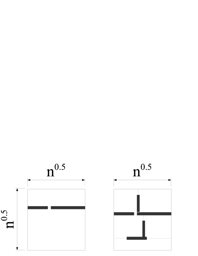
Figure 10: A set of doubling network topologies. The network is dense, and made inhomogeneous by the walls, which do no allow transmissions to go through. Note that the walls stretch when $n$ grows, such that the network wide distortion also grows with $n$. Dashed lines indicate the separation into sets.

III-B Sequences of Communication Graphs

In this subsection we study the behavior of a sequence of communication graphs, without any obstacles. We show that a sequence of $\mathcal{G}^{(t)}(n,r_{n})$ of length $n^{\rho}$, for some constant $\rho$, with the USL mobility model is $\kappa$-smooth. As already seen in Theorem 4, such a sequence of graphs is doubling at every time instant.

Theorem 10

A sequence of $\mathcal{G}^{(t)}(n,r_{n})$ of length $\leq n^{\rho}$, where nodes move according to the USL mobility model with maximum constant speed $S$ is

$$max\left\{\frac{r_{n}d^{(t)}}{\frac{r_{n}d^{(t)}}{\sqrt{5}\sqrt{2}}-2\sqrt{5}\sqrt{2}\tau S},\sqrt{5}\sqrt{2}(1+\frac{2\tau S\sqrt{5}\sqrt{2}}{r_{n}d^{(t)}})\right\}$$

smooth w.h.p.

Proof:

Consider two nodes $u$ and $v$ at Euclidean distance $q_{2}^{(t)}=||x_{u}-x_{v}||_{2}$ at time $t$. Let $q_{1}^{(t)}=||x_{u}-x_{v}||_{1}=\sum_{m=1}^{2}|x_{m}(u)-x_{m}(v)|$. Further, denote by $d^{(t)}=\mbox{$d^{(t)}$}(u,v)$ their shortest path distance at time $t$. One can see that $\frac{q_{2}^{(t)}}{r_{n}}\leq\mbox{$d^{(t)}$}\leq\frac{\sqrt{5}\sqrt{2}q_{2}^{(t)}}{r_{n}}$. Indeed, the shortest possible path will follow a straight line between $u$ and $v$. The length of this line is $q_{2}^{(t)}$ and one hop can be of length at most $r_{n}$. In the worst case, the shortest path from $u$ to $v$ will follow the shortest path in the grid formed by the small squares of side $\frac{r_{n}}{c}=\frac{r_{n}}{\sqrt{5}}$, which exists w.h.p. Recall that we can only guarantee horizontal and vertical connectivity between small squares. The number of small squares in this path will be at most $\frac{\sqrt{5}q_{1}^{(t)}}{r_{n}}$. One can easily show that $q_{1}^{(t)}\leq\sqrt{2}q_{2}^{(t)}$. Let $x=\left(\begin{array}[]{c}x_{1}\\ x_{2}\end{array}\right)=\left(\begin{array}[]{c}x_{1}\\ sx_{1}\end{array}\right)=(x_{u}-x_{v})$. We have

$$\begin{array}[]{ll}q_{2}^{(t)}&=\sqrt{x_{1}^{2}+x_{2}^{2}}=x_{1}\sqrt{1+s^{2}}\\ &=(1+s)x_{1}\frac{\sqrt{1+s^{2}}}{1+s}=q_{1}^{(t)}\frac{\sqrt{1+s^{2}}}{1+s}.\end{array}$$

Since, we have $\frac{q_{2}^{(t)}}{q_{1}^{(t)}}=\frac{\sqrt{1+s^{2}}}{1+s}$, the term is maximized when $s=1$. In Figure 11, we illustrate this point.

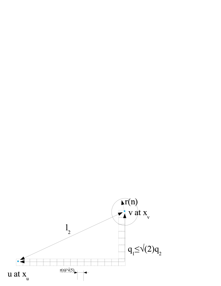
Figure 11: Upper and lower bounds for the shortest path

Similarly, at time $t+\tau$, the shortest path distance will be bounded by $\frac{q^{(t+\tau)}_{2}}{r_{n}}\leq d^{(t+\tau)}\leq\frac{\sqrt{5}\sqrt{2}q^{(t+\tau)}_{2}}{r_{n}}$. However, we know that the Euclidean distance can change by at most $2\tau S$ in $\tau$ time steps. Consequently,

$$\frac{q_{2}^{(t)}-2\tau S}{r_{n}}\leq d^{(t+\tau)}\leq\frac{\sqrt{5}\sqrt{2}(q_{2}^{(t)}+2\tau S)}{r_{n}}$$ (3)

We can now bound the multiplicative stretch as follows: Hence,

$$\begin{array}[]{l}max\left\{(\frac{1}{\sqrt{5}\sqrt{2}}-\frac{2\tau S}{\sqrt{5}\sqrt{2}q_{2}^{(t)}})^{-1},\sqrt{5}\sqrt{2}(1+\frac{2\tau S)}{q_{2}^{(t)}})\right\}\\ =max\left\{\sqrt{5}\sqrt{2}\frac{q_{2}^{(t)}}{q_{2}^{(t)}-2\tau S},\sqrt{5}\sqrt{2}(1+\frac{2\tau S}{q_{2}^{(t)}})\right\}\\ =max\left\{\frac{r_{n}\mbox{$d^{(t)}$}}{\frac{r_{n}\mbox{$d^{(t)}$}}{\sqrt{5}\sqrt{2}}-2\sqrt{5}\sqrt{2}\tau S},\sqrt{5}\sqrt{2}(1+\frac{2\tau S\sqrt{5}\sqrt{2}}{r_{n}\mbox{$d^{(t)}$}})\right\}=\kappa(\tau,d)\end{array}$$

∎

One can now observe that the time it takes to multiply the shortest path distance between two nodes at distance $d$ is proportional to $d$. Note that the larger the communication radius $r_{n}$, the smaller $\kappa$. Hence, the distance grows at most linearly with time. In particular, we have:

Corollary 2

There exist constants $\nu$ and $\kappa$ defined in the proof such that a sequence of $n^{\rho}$ connectivity graphs, under the USL mobility model with maximum constant speed $S$, is $\kappa$-smooth w.h.p.

Proof:

By theorem 10, we know that the sequence is

$$max\left\{\frac{r_{n}\mbox{$d^{(t)}$}}{\frac{r_{n}\mbox{$d^{(t)}$}}{\sqrt{5}\sqrt{2}}-2\sqrt{5}\sqrt{2}\tau S},\sqrt{5}\sqrt{2}(1+\frac{2\tau S\sqrt{5}\sqrt{2}}{r_{n}\mbox{$d^{(t)}$}})\right\}$$

-smooth w.h.p. Note that both terms decrease as a function of the communication radius $r_{n}$. Hence, we can set $r_{n}=1$ without decreasing $\kappa(\tau,d)$. Similarly, both terms go down when the distance $d^{(t)}$ goes up. We can therefore also set $\mbox{$d^{(t)}$}=1$, which is the smallest possible distance in an unweighted graph. Consequently, if we set $\tau=\nu\mbox{$d^{(t)}$}=\nu$, we can now write

$$\kappa(\tau,d)\leq max\left\{\frac{1}{\frac{1}{\sqrt{5}\sqrt{2}}-2\sqrt{5}\sqrt{2}\nu S},\sqrt{5}\sqrt{2}(1+2\nu S\sqrt{5}\sqrt{2})\right\}$$

which is constant for $\nu$ constant. ∎

IV Routing Algorithm

We develop the routing algorithm and its performance analysis for a general class of dynamic networks which produce a sequence of doubling and smooth connectivity graphs. We have seen in Sections II and III that this applies to a class of wireless connectivity models with USL mobility. For notational convenience we illustrate the ideas for a sequence $\mathcal{G}^{(t)}(n,r_{n})$ geometric random graphs with USL mobility.

We decompose a time step into two phases: a beaconing phase and a forwarding phase. In the former phase, a set of routes are established by letting all or a subset of nodes flood the network at geometrically decreasing radii and nodes register with beacon nodes. In the latter phase, this subset of routes is then utilized by source nodes to efficiently search for the destination. Every node is equipped with a routing table as shown in Table II.

Node identifier	distance $\left[hops\right]$	level	next hop
⋮	⋮	⋮	⋮

TABLE II: Routing Table RT

We first describe two procedures used in the beaconing and the routing phase.

flood(R,level) procedure: When a node $u$ initiates the $flood(R,level)$ procedure, it broadcasts a flood packet as shown in Table III to its direct neighbors in $\mathcal{G}(n,r_{n})$. The hop count field is initialized to $0$ and the content of the Level field is set to the level of the beacon. How the level of the beacon is determined will be specified in the sequel. All nodes can compute the maximum hop count given the value of the level field in the packet.

Pkt. Type	Node Id.	Hop Count	Level
$O(1)$ bits	$O(\log n)$ bits	$O(\log n)$ bits	$O(\log\Delta)$ bits

TABLE III: Flood Packet

The neighbors which receive this packet, after increasing the hop count by $1$, add an entry to their routing table for node $u$ if no entry for the same node and level with lower or equal hop count is present in the RT. The next hop field is set to the identifier of the node from which the packet was received. The level field in the routing table is set to the level given in the packet. In turn, the nodes which got the packet from $u$ broadcast this packet to their neighbors. The latter follow the same procedure and update the routing table if necessary. The packet is discarded when the hop count reaches the maximum hop count (which is a function of the level). Note that with this procedure, every node forwards the packet at most once and the distance added to the routing table is the shortest path distance in $\mathcal{G}(n,r_{n})$. This procedure also allows us to establish a reverse path from all nodes that get the packet back to $u$. Indeed, it suffices for all these nodes to store the identifier of the node from which they received the packet. Further, for any node $v$, that reverse path a shortest path to $u$.

probe(relay,destination) procedure: This procedure consists in sending a probe packet (see Table IV) to a “relay” node for which the source has an entry in its routing table. The relay node will set the success bit to $1$ if it has an entry for the destination and $0$ otherwise. We will make sure that all nodes on the path between the source and the relay node have an entry for the relay node in their routing table. Additionally, nodes on the path add a temporary entry for the source in the routing table. They set the next hop field to the identifier of the node from which they received the packet and leave the level and distance field empty.

Pkt. Type	Relay Id.	Dest. Id.	Success
$O(1)$ bits	$O(\log n)$ bits	$O(\log n)$ bits	$1$ bit

TABLE IV: Probe Packet

Upon receiving the packet, the relay node can either answer to the source on the reverse path we just created if the answer is negative. Alternatively, it can take action as explained in the sequel if it has an entry for the destination.

We now separately detail the beaconing and the routing algorithms underlying our routing protocol

IV-A Beaconing Algorithm

In this subsection, we start by describing the first time step, when nodes have not yet moved and no information has been exchanged. In a static network, the information exchanged in this first step would be sufficient to setup a complete routing infrastructure. On the other hand, in a mobile environment, we would need to cope with the dynamic topology and constantly update the routing tables. How we deal with a dynamic environment is explained at the end of the subsection. Let the cover radius at level $i$, for $i=1,...,\log\Delta$ ($\Delta$ being the diameter of the network), be defined as $r_{i}=2^{i}$ and the flooding radius at level $i$ be defined as $f_{i}=\kappa(r_{i+1}+r_{i})$, where $\kappa$ is a constant chosen such that $\kappa(\nu d,d)\leq\kappa d$, $\forall d$. In order for the routing algorithm to work properly, it is crucial that beacons at level $i$ are within the flooding radius of the beacons at level $i+1$, if they have common nodes inside their cover radii (see Fig. 12).

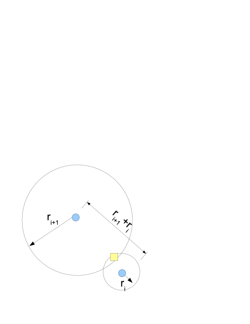
Figure 12: The flooding radius is chosen in such a way that beacons at level $i$ hear the floods of beacons at level $i+1$. In static networks, this is $r_{i}+r_{i+1}$.

This is why we define the flooding radius above. Note that if the network is static, we can set $\kappa$ to $1$. Else, the value of $\kappa$ depends on how mobile the nodes are (see Def. 6).

The idea of the algorithm is to build a hierarchical cover of the network i.e., we would like every node in the network to be within $r_{i}$ hops of a beacon node at every level $i$. We say that when a node is within $r_{i}$ of a beacon $b$ at level $i$, it is a member of $b$’s cluster at level $i$, but it can only be in one cluster at every level. To achieve this, we let the nodes flood in a random order which can change at every time step. Every node $u$ is a beacon at a given level $\beta(u)$. The flooding radius, however, will depend on the highest level at which a node is not covered. Let us denote by $h(u)$ the highest level at which node $u$ is not covered. When node $u$’s turn to flood comes, it will determine the value of $h(u)$ set $\beta(u)=h(u)$ and call $flood(f_{h(u)},h(u))$. A node $v$ which receives this flood will determine the lowest level at which it could be a member of $u$’s cluster, say $l(v)$. That is, it will determine the lowest value $j$ for $l(v)$ such that $d(u,v)\leq 2^{j}$. This distance $d(u,v)$ is known since $v$ just received a flood packet from $u$. It will then become a member of $u$’s cluster for all levels above $l(v)$ for which it has no membership yet and are below $\beta(u)$. If a node becomes a member of $u$’s cluster, it sends a membership packet (see Table V)

Pkt. Type	Node Id.	Beacon Id.	Level
$O(1)$ bits	$O(\log n)$ bits	$O(\log n)$ bits	$O(\log\Delta)$ bits

TABLE V: Membership Packet

back to $u$. In this way, $u$ learns the identifier of all nodes in its cluster. Note that $u$ also applies this procedure to itself, and consequently could be a beacon at level $i$ but not at level $j<i$.

The control traffic will be dominated by the messages sent back by nodes to beacons when they become members of a cluster, so should be rare. Moreover, we do not want the distance between a node and its beacon to grow by more than a constant factor. Since we assume that the maximum speed of the node is constant, the higher the level of a beacon, the more time it will take for nodes to double their distance to this beacon. We want to elect new beacons and update memberships only for levels at which the distances could have been multiplied by a constant factor. Recall that the network is $\kappa$-constrained. Consequently, the distance $\mbox{$d^{(t)}$}(u,v)$ between two nodes $u$ and $v$ cannot change by a factor $\kappa$ in less than $\nu d$ time steps (see Corollary 2). In particular, if a node is at distance $2^{i}$ of a beacon at the time it becomes a member of its cluster, then we have $d^{t+\nu 2^{i}}\leq\kappa 2^{i}$. Hence, we update the memberships at level $i$ only every $\nu 2^{i}$ time steps (see Figure 13).

Figure 13: The memberships up to level $i$ are updated every $\nu 2^{i}$ time steps. At the levels above, beacons elected at earlier time steps simply flood again.

This will lead to a routing scheme in which the distances can be distorted by at most a constant factor to be calculated in the sequel. Additionally, in a dynamic environment, routes can break. This is why we let the beacons at all levels flood at every time step. Levels at which no membership updates take place simply use the floods of the beacons to update their routes toward theses beacons. This will ensure that a route always exists for all pair of nodes.

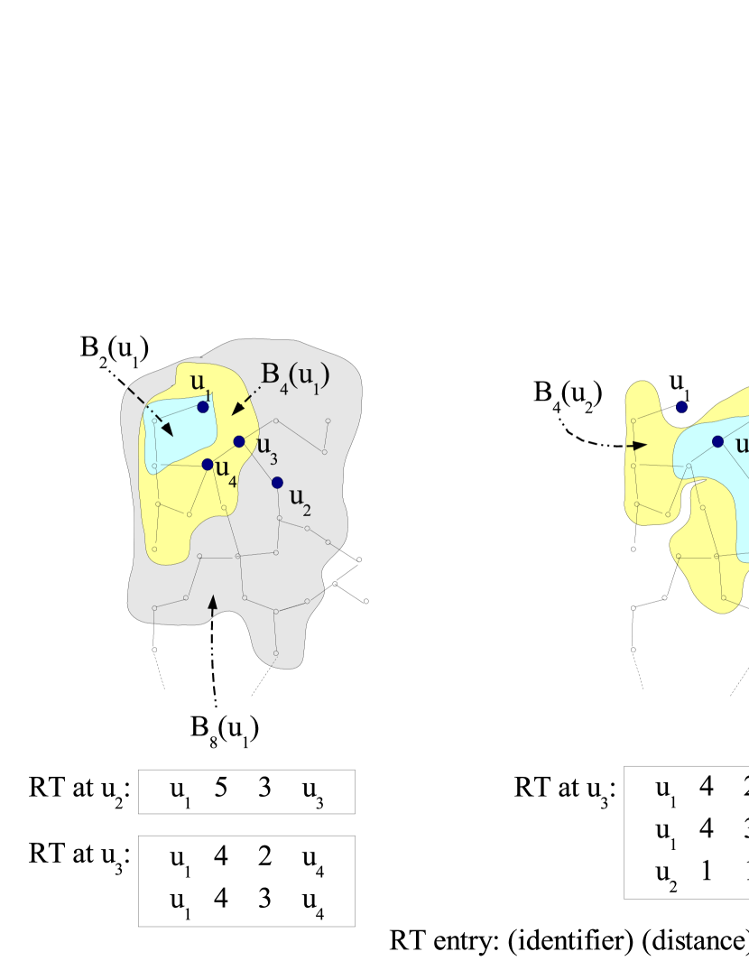
Figure 14: The example start with empty routing tables. First, on the left, node $u_{1}$ floods at level $3$. We focus on nodes $u_{2}$ and $u_{3}$. Node $u_{2}$ is within $8$ hops from $u_{1}$ but further away than $4$ hops. Consequently, it can only had an entry for node $u_{1}$ at level $3$. At the same time, node $u_{3}$ can add an entry for node $u_{1}$ at the levels $2$ and $3$, since it is at distance $4$ of $u_{1}$. Next, on the right, $u_{2}$’s turn to flood comes (right after $u_{1}$’s turn). This node is already covered at level $3$. Consequently, it will flood at level $2$. The node $u_{3}$ could potentially add an entry for this node at levels $1$ and $2$. However, it is already covered at level $2$ and so adds only an entry for level $1$. We do not show the entries beacons add for themselves.

In Figure 14, we give a simple with three levels. The beaconing algorithm is presented in Algorithm 1. It is important to note that the routes are updated at every time step and consequently routing toward a beacon will always be successful. Further, when the membership at a given level $i$ is updated, all the memberships at the levels $j<i$ will also be updated, and all memberships at these levels canceled.

Data: Routing Table, Time t

begin  Let $\Gamma=\max\left\{0\leq j\leq\log\Delta|t\ mod\nu 2^{j}=0\right\}$;

Clear routing table entries with $level\leq\Gamma$;

Let $\beta(u)$ be the level at which $u$ is a beacon;

if $\pi(\ell)=u$ then  if $\beta(u)\leq\Gamma$ then  Let $h(u)$ be the highest level at which $u$ is not covered;

$\beta(u)=h(u)$; end $flood(f_{h(u)},h(u))$;

end end

Algorithm 1 Beaconing Algorithm at node $u$

IV-B Forwarding Algorithm

The forwarding algorithms works as follows: a source node $u$ with a message for a target node $v$ searches for $v$ by first probing all the level 1 beacon it knows of. To do so, it looks at its routing table and selects all nodes it knows of at level $1$. If all answers are negative, node $u$ probes all level $2$ beacons it knows of. The procedure is repeated as long as all beacons answer negatively. A beacon at level $i$ with an entry for the destination in its routing table does not answer directly to the source. Rather, this node will search downwards in the hierarchy by probing all the level $i-1$ beacons it knows of. We show in the next section that one of these beacons must have an entry for the destination. That beacon in turn probes all the beacons in knows of at level $i-2$. Meanwhile, the other beacons at level $i-1$ will answer negatively to the beacon at level $i$. The procedure is repeated recursively until the target itself is reached. The target will then answer to the source on the reverse path which will later be used for communication between the source and the destination. To summarize, the forwarding algorithm starts with an “upstream” phase during which the source node probes beacons level by level until a beacon is found which has the destination in its cluster. That beacon then starte a “downstream” phase, during which we go down in the hierarchy. We illustrate the forwarding procedure conceptually in Figure 15.

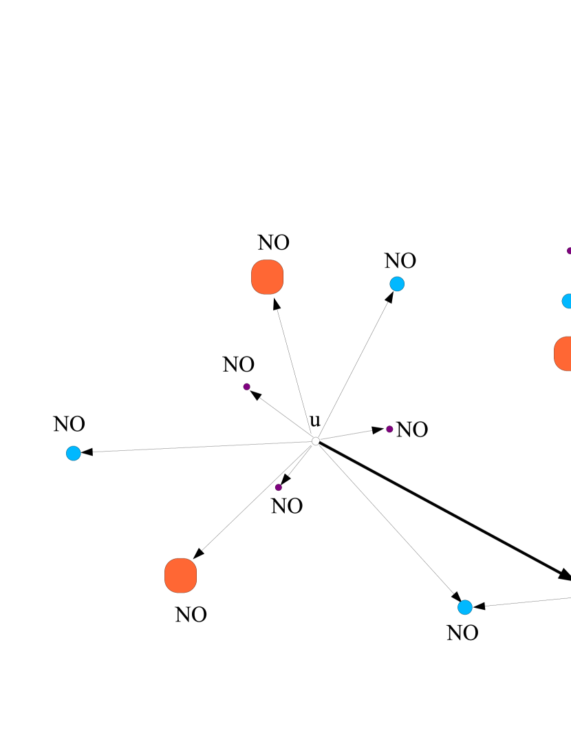
Figure 15: Node $u$ has a packet for node $v$. It searches in its routing table for all beacons it knows of at level $1$ and sends them a probe packet containing $v$’s identifier. None of the beacons at level $1$ has an entry for this node and consequently they all answer negatively to node $u$. Next, node $u$ repeats the same procedure with all the beacons it knows of at level $2$. Again, all beacons answer negatively. On the third level, now, a beacon has an entry for node $v$. This beacon will probe all the beacons it knows of at level $2$, while the other beacons at level three will answer negatively to $u$. A beacon at level $2$ must have an entry for $v$. This beacon again probes all the beacons it knows of at level $1$ among which one must have an entry for $v$ itself. Meanwhile, the other beacons reply negatively as they do not have any entry for $v$.

IV-C Load-balancing

This approach above guarantees a low network wide control traffic overhead. Even though over a long period of time all nodes will get approximately the same average overhead, beacons at the highest levels might get overloaded by the membership packets of the nodes in their cluster when a membership update takes place. These nodes will be hot spots in the network for a short period of time. To work around this problem, memberships can be distributed in the cluster instead of stored at the beacon itself. First, we now set $f_{i}^{\prime}=\kappa(2r_{i+1}+r_{i})$. Additionally, whenever a beacon floods at level $i$, it includes its membership at level $i+1$ in the packet. This information is stored by all nodes that receive this flood packet. This will guarantee that all nodes that are members of a cluster at level $i$, know how to reach all beacons at level $i-1$ inside that cluster. A node that becomes a member of the cluster of beacon $b_{i}(u)$ at level $i$ will now send its membership packet directly toward the beacon $\psi_{i-1}(u)$ at level $i-1$ inside this cluster with the identifier closest to $u$’s. In turn, as soon as the packet reaches a node which is a member of $\psi_{i-1}(u)$’s cluster at level $i-1$, the membership packet is redirected toward the beacon $\psi_{i-2}(u)$ which is a member of $\psi_{i-1}(u)$’s cluster at level $i-1$ and has the identifier closest to node $u$’s. The process is repeated until we reach a single node, which will store $u$’s identifier on behalf of $b_{i}(u)$. Note that the membership can only be registered at a single location in the cluster reachable through a unique sequence of clusters. This remains true even when nodes move. Indeed, the nodes in the cluster of $b_{i}(u)$ will only forward the packet to beacons at level $i-1$ which were in the same cluster at the time the membership for this level got updated. Of course, whenever level $j<i$ is updated, we do now not only need to send $u$’s identifier toward its new beacon at that level. Additionally, the node that holds $u$’s identifier at level $j$ might not be reachable anymore through a path of clusters with identifiers closest to $u$’s. Consequently, this node will need to forward $u$’s identifier toward the beacon at level $j$ with the identifier closest to $u$’s. Again the process will be repeated recursively until a single node is reached. As we will see, the cost of avoiding hot spots is a factor $\log{n}$ in the total control traffic. Finally and most importantly, with this procedure beacons no longer get overloaded. Rather, the traffic is be distributed in its cluster.

The data forwarding process remains the same except that the source node will not probe the beacon itself, but rather search for the node in the beacon’s cluster that should hold the destination’s identifier. If this node holds the identifier, it will then probe the beacons one level below in the same way. Recall that the nodes which potentially hold $u$’s membership can be reached at any given instant in time through a unique sequence of clusters. The procedure is repeated until the destination is reached.

V Performance Analysis

In this section, we analyze the performance of our algorithm analytically both in terms of control traffic and of route stretch. As in Section IV, we do this for a sequence of doubling and smooth connectivity graphs, and will use $\mathcal{G}^{(t)}(n,r_{n})$ with USL mobility for illustration.

The bounds derived in this section hold w.h.p. when we are in a sequence of length $n^{\rho}$ of $\alpha$-doubling connectivity graphs. In the sequel, $\alpha$, $\kappa$ and $\nu$ are the constants derived in Section III. Let us denote by $\Delta=O(\sqrt{(}\frac{n}{\log(n)}))$ the diameter of the network. To bound the control traffic necessary for beaconing, we will rely on the $\alpha$-doubling property of the metric space to show that a node can only hear a constant number of beacons at every layer. We will first show that a ball of radius $2R$ around any node $u$ can only contain at constant number of balls (clusters) of radius $R$, when we select the centers of the balls of radius $R$ in an arbitrary order and ensure that two centers cannot be closer than $R$. We will later use this result to show that a node can hear at most a constant number of beacons at any given level.

Theorem 11 (Random Cover)

Let $\mathcal{B}_{2R}^{X}(u)$ be a ball of radius $2R$ centered at $u$ in a graph metric $(X,d)$ with doubling constant $\alpha$. Then, there exist at most $k\leq\alpha^{2}$ nodes $v_{i}$, $(i=1,2,..,k)$ such that $\mbox{$\mathcal{B}_{2R}^{X}(u)$}\subseteq\bigcup_{i}^{k}\mbox{$\mathcal{B}_{R}^{X}(v_{i})$}$ and $min_{(i,j)}d(v_{i},v_{k})>R$.

Proof:

By definition of an $\alpha$-doubling metric space, there must exist a cover of a ball of radius $2R$ consisting of at most $\alpha$ balls of radius $R$. Recursively, there must also exist an $\frac{R}{2}$-cover consisting of $\alpha^{2}$ points. One can select at most one center $v_{i}$ in each ball of radius $R/2$, as any other point inside this ball is within $R$ of $v_{i}$. Hence, one can select at most $\alpha^{2}$ such centers. ∎

Corollary 3

Let $B$ be a ball of radius $R>R^{\prime}$ in an $\alpha$-doubling metric space $(X,d)$. Then, one can select at most $k\leq(\frac{R}{R^{\prime}})^{2log(\alpha)}$ nodes $v_{i}$, $(i=1,2,..,k)$ such that $\mbox{$\mathcal{B}_{R}^{X}(u)$}\subseteq\bigcup_{i}^{k}\mbox{$\mathcal{B}_{R^{\prime}}^{X}(v_{i})$}$ and $min_{(i,j)}d(v_{i},v_{j})>R^{\prime}$. In particular, if $R=\eta R^{\prime}$ for some constant $R$, then $k$ is at most a constant $(\eta)^{2log(\alpha)}$ independent of $n$.

Proof:

Let $R=2^{i}R^{\prime}$. Hence, $R^{\prime}$ is doubled $log\frac{R}{R^{\prime}}$ times to obtain $R$. By Theorem 11, $B$ can be covered by $\alpha^{2log\frac{R}{R^{\prime}}}=(\frac{R}{R^{\prime}})^{2log(\alpha)}$ balls of radius $R^{\prime}$. ∎

Here, one can think of the radius $R$ of the large balls as the flooding radius, and of the radius $R^{\prime}$ of the small balls as the cover radius. Indeed, we use this result to show that a node $u$ can hear the floods of all beacons within a given radius $R$. Moreover, this ball of radius $R$ can contain at most $(\frac{R}{R^{\prime}})^{2log(\alpha)}$ beacons, since beacons must be at least $R^{\prime}$ apart.

V-A Control Traffic

Theorem 12

The average control traffic overhead per time step for beaconing is at most $O(n\log^{2}n)$ bits.

Proof:

We will analyze the control traffic at level $i$. Recall that a beacon at level $i$ floods a distance $f_{i}=\kappa(2^{i+1}+2^{i})$ at every time step. Further, at the time the memberships are updated at level $i$, a beacon node at this level cannot be within $r_{i}=2^{i}$ of another beacon at that level. If it were the case, this node would not elect itself as a beacon at this level. Level $i$ is updated every $\nu 2^{i}$ time steps. Consider a node $u$. By Corollary 10, no nodes that are further away than $\kappa f_{i}$ hops at the time the memberships are updated at level $i$ could move within $f_{i}$ of $u$ in less than $\nu 2^{i}$ time steps. However, that is before this level is updated again. Consequently, the number of beacons whose flood can reach $u$ at any given time step is at most the number of level $i$ beacons in a ball of radius $\kappa f_{i}$ at the time the membership is updated. In turn, node $u$ will broadcast the flood packets of at most that many beacons for this level $i$. By Corollary 3, this number is a constant given by $(\frac{\kappa f_{i}}{2^{i}})^{2log(\alpha)}=(3\kappa^{2})^{2\log\alpha}$. Given that there are $O(\log n)$ levels, that there are $n$ nodes and that a flood packet has size $O(\log n)$ bits, the average control traffic overhead per time step for beaconing is at most $O(n\log^{2}n)$ bits. ∎

We now compute the control traffic overhead necessary for nodes to update their memberships with beacons. Recall that level $i$ and all levels below are updated every $\nu 2^{i}$ times steps and that a node can only be a member of one cluster at every level. Furthermore, a node only becomes a member of a cluster if it is within $2^{i}$ of the corresponding beacon.

Theorem 13 (Membership Update Overhead)

The average control traffic overhead per time step to update memberships without load-balancing is at most

$$\frac{n\log\Delta\log n}{\nu}=O(n\log^{2}n)$$

bits.

Proof:

Consider a sequence of $T$ time steps. The memberships will be updated up to level $i$ every $\nu 2^{i}$ time steps, so $\frac{T}{\nu 2^{i}}$ times in a sequence of length $T$. At the time of the update, a node can be at distance at most $2^{i}$ from a beacon at level $i$. Consequently, the overhead in bits generated by a node in a sequence of $T$ time steps is upper bounded by $\sum_{i=1}^{\log\Delta}\frac{T}{\nu 2^{i}}2^{i}\log n=\frac{\log\Delta}{\nu}\log n$. ∎

Finally, we will show that the average control traffic overhead when load-balancing is used is increased by at most a factor $\log n$.

Theorem 14 (Membership Update Overhead)

The average control traffic overhead per time step to update memberships with load-balancing is at most

$$\frac{n\log^{2}\Delta\log n}{\nu}=O(n\log^{3}n)$$

bits.

Proof:

Consider a sequence of $T$ time steps. The memberships will be updated up to level $i$ every $\nu 2^{i}$ time steps, so $\frac{T}{\nu 2^{i}}$ times in a sequence of length $T$. At the time of the update, a node can be at distance at most $2^{i+1}$ from a beacon at level $i-1$ inside its cluster at level $i$. Similarly, a node can be at distance at most $2^{i}$ from a beacon at level $i-2$ inside its cluster at level $i-1$. In the load balanced scheme, we have to count the overhead to go down the hierarchy of beacons. For a beacon at level $i$, this is at most $2^{i}\times 2$. Consequently, the overhead in bits generated by a node in a sequence of $T$ time steps is upper bounded by $4\sum_{i=1}^{\log\Delta}\frac{T}{\nu 2^{i}}2^{i}\log n=4\frac{\log\Delta}{\nu}\log n$. However, node $u$ is a member of a cluster at all $\log{\Delta}$ levels. Recall that the node that holds $u$’s identifier must always be reachable through a path by choosing the beacon (cluster) with the identifier closest to $u$’s. Hence, whenever level $i$ gets updated, all $\log{\Delta}$ nodes that hold $u$’s identity must follow the same procedure as $u$ itself. We conclude that the overhead is upper bounded by $\log{\Delta}4\frac{\log\Delta}{\nu}\log n$ bits. ∎

V-B Route Stretch

In this section we will show that the route found with the forwarding algorithm is only a constant factor longer than the shortest path. Additionally we show that the destination location discovery takes a negligible fraction of a flow throughput.

Theorem 15 (Routing Stretch)

The worst case multiplicative routing stretch is $O(1)$.

Proof:

We first analyze the stretch without load balancing. Consider that we want to route from a node $u$ to a node $v$, and that we had $2^{k}\leq d(u,v)\leq 2^{k+1}$, the last time level $k$ was updated before the route search takes place. Let us denote by $b_{i}(v)$ the beacon to which node $v$ had registered the last time level $i\leq k$ was updated before the route search takes place. Clearly, we have $d(u,b_{v}(k))\leq\kappa(2^{k+1}+2^{k})$, and $d(b_{i}(v),b_{i-1}(v))\leq\kappa(2^{i}+2^{i-1})$. This is true since the membership of node $v$ at level $i$ must have been updated at most $\nu 2^{i}$ time steps before the routing takes place, and that at the time the time level $i$ gets updated, we have $d(b_{i}(v),b_{i-1}(v)))\leq d(b_{i}(v),v)+d(v,b_{i-1}(v))$ by triangle inequality. Note that $d(b_{i}(v),b_{i-1}(v))\leq f_{i-1}$ and that $d(u,b_{v}(k))\leq f_{k}$. Hence, a route must exist between $u$ and $v$ and the length $r^{(t+\tau)}(u,v)$ of the route at time $t$ is at most:

$$\begin{array}[]{ll}r^{(t)}(u,v)&\leq\sum_{i=1}^{k}f_{k}=\kappa\sum_{i=1}^{k}(2^{i+1}+2^{i})\\ &=3\kappa\sum_{i=1}^{k}2^{i}=3\kappa\frac{2^{k+1}-1}{2-1}\leq 6\kappa d^{(t)}(u,v)\end{array}$$

In the worst cast, nodes $u$ and $v$ have moved closer together (by a factor $\kappa$) while the beacons have moved further apart. Indeed, we have $d^{(t+\tau)}(u,v)\leq\kappa d^{(t)}(u,v)$ for $\tau\leq\nu 2^{k}$ as our network is $\kappa$-constrained. Note that if we waited longer that $\nu 2^{k}$, memberships would be updated again at level $k$ and we could find another beacon at distance $2^{k}$ at most from $v$ at level $k$. Hence, the worst case stretch is $\frac{r^{(t+\nu 2^{k})}(u,v)}{d^{(t+\nu 2^{k})}}\leq 6\kappa^{2}=O(1)$. ∎

Every node can only hear floods from a constant number ($\mu=(3\kappa^{2})^{2\log\alpha}$, see Theorem 12) of beacons at every level. Recall that the source will first probe all beacons at level $1$, then all beacons at level $2$ and so on. The procedure is repeated up to level $k$ at which the source $u$ will send a packet to $b_{k}(v)$. Note that the distance from $u$ to this beacon can be at most $\kappa 2^{k+1}+2^{k}=f_{k}$ and so it must hear its floods. In turn, when routing down the hierarchy, beacon $b_{j}(v)$ will probe at most a constant number ($(3\kappa^{2})^{2\log\alpha}$ of beacons at level $j-1$. Finally, the distance between a node $u$ and a beacon at level $i$ can be at most $f_{i}$ and a probe packet will traverse at most $2f_{i}$ packets when a beacon at level $i$ is probed (back and forth). This means that for discovery of the location of the destination, we need a probe overhead of at most $\mu 6\kappa d(u,v)$ packet transmissions. Therefore, this is a negligible part of the throughput of a flow since it consumes roughly the equivalent of a few packet headers of a flow from source to destination. A similar statement can be made for the load-balanced case.

VI Implementation Issues

In Section V, we have computed worst case bounds which may be conservative in terms of constants. In this section, we explore this aspect by looking at simulation results for the control traffic and for the stretch. Recall that we had computed that for each of the $O(\log n)$ levels, a node has to retransmit a packet of at most $(3\kappa^{2})^{2\log\alpha}$ beacons. Even if we set the maximum speed as well as the parameter $\nu$ to $1$, this is still $\sqrt{10}+20$ and consequently the constant in the bound on the overhead at least as high as $(3(\sqrt{10}+20)^{2})^{2}\approx 2.5\cdot 10^{6}$! In Figure 16, however, we show that in practice this constant is approximately 30. This simulation was run with $50$ up to $10000$ nodes moving at a maximum speed of $1$. One can observe that the experimental scaling behavior corresponds extremely well to the theoretical behavior. To stress this fact, we also plot $100\log n$ as a benchmark. Note that the overhead is expressed in number of packets rather than bits (a packet being of size $O(\log n)$).

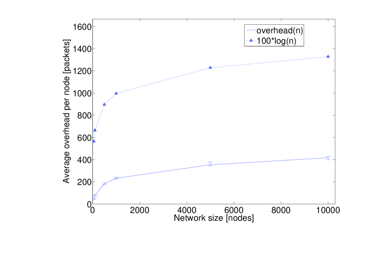
Figure 16: Average control traffic overhead per node in packets as a function of the network size. Nodes move at a speed of maximum speed of $1$. The confidence interval is given by the 95% and 5% percentiles. The size of a packet is $O(\log n)$ bits. We also plot $100\log{n}$ to show that our analytical predictions match the simulation results.

Similarly, in Figure 17 we show that for a network of $1000$ nodes, the stretch is at most $1.5$ for all node pairs. If we compute the maximum theoretical stretch, we can show that it is again considerably larger and hence a pessimistic bound. These small constants could make a practical implementation realistic.

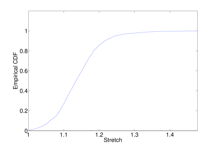
Figure 17: Empirical cumulative distribution of stretch (route length/shortest path) for a network with $1000$ nodes moving at a maximum speed of $1$.

We have made a certain number of assumptions in our models, which we now clarify. In practice, the random permutations on the nodes, which determines the order in which the flooding occurs, could be implemented by using random timers; more precisely, by letting all nodes draw a random delay independently of each other every $\Delta T$ seconds. Obviously, the interval from which nodes draw this delay should be made sufficiently large so that we can avoid collisions. However, a level in the hierarchy will be rapidly covered, and in a practical implementation the covers at different levels could be built in parallel. Further, different parts of the network are independent except at the highest level, and we could exploit this spatial diversity to parallelize the beaconing process. Hence, we speculate that it is possible to reduce the length of the beaconing phase to a small constant times the maximum round-trip time. Note that one could apply the algorithms to underlying networks that are not doubling. In this case, we would not be able to give provable bounds on the control overhead and the stretch as we did for doubling networks.

VII Conclusions

In this paper, we show that a large class of wireless network models belong to a larger class of networks, the doubling networks, in which efficient routing can be achieved. To design an efficient routing scheme, one can hierarchically decompose the network by relying on the doubling property to prove that the control traffic overhead and the stretch will remain low, even for dynamic doubling networks. This holds for a fairly broad class of uniform speed-limited (USL) mobility models. One advantage of the proposed routing algorithm is that it is robust, in that it works well in certain situations in which other existing algorithms cannot work well. This was illustrated in Section II-A for an example network with obstacles. We believe that many more such examples can be created where the use of the doubling rather than geographic properties would be crucial. To the best of our knowledge, our results are the first provable bounds for routing quality and costs for dynamic wireless networks. These techniques might give us insight into algorithm design for more sophisticated wireless network models.

Unit Disc Graphs

Another common model used in studies on wireless networks are Unit Disk Graphs (UDG), which are the deterministic variants of the random geometric graphs. The randomness of the positions of the nodes is removed and they can be placed arbitrarily on a finite of infinite area. The channel model is completely deterministic as before and nodes are connected if their Euclidean distance is below a threshold distance $r$, called the communication radius. In mathematical terms, two nodes $u$ and $v$ with positions $x(u),x(v)\in[0,R]^{2}$ are connected if and only if $||x(u)-x(v)||<r$. We will now show that there exist UDG which are not $\alpha$-doubling (see Section II for a definition of an $\alpha$-doubling metric).

Theorem 16

There exists an infinite UDG for which is no constant that upper bounds the doubling dimension i.e., UDG are not doubling.

Proof:

Consider the graph shown in Figure 18.

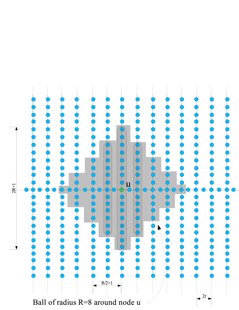
Figure 18: An infinite UDG obtained by deleting all the nodes in every second column of a grid, except for the nodes on the the middle row. Consequently, “columns” are $2r$ apart.

To show that this graph is not $\alpha$-doubling, we must show that there exists no constant such that all balls of radius $R$ can be covered a constant $\alpha$ number of balls of radius $R/2$, for all $R$. Consider the ball centered around $u$ in the figure. One can see that there are $R/4+1$ “columns” which cross the middle row at a distance less than $R/2$ from $u$ (that is, the intersection of the column and the row is less than $R/2$ hops away from $u$). The intersection of each of these columns with $B_{u}(R)$ is of length more than $R$ (see hatched zones on Figure 18). Consequently, for each of these columns there is at least one node at distance more than $R/2$ from the middle row. To cover these nodes, we need to place at least one ball of radius $R/2$ on each of these columns. Hence, the doubling dimension is lower bounded by $R/4$ and tends to infinity as $R$ goes to infinity. ∎

One can notice that in the non-doubling UDG in the proof of Theorem 16 results from a careful construction. In Appendix Random Geometric Graphs with $r_{n}<\sqrt{\log n}$, we show however that such a structure will occur with high probability when $r_{n}<\sqrt{\log n}$ in random geometric graphs.

Random Geometric Graphs with $r_{n}<\sqrt{\log n}$

We first consider the case in which the communication radius $r$ is such that $r_{n}=r=(\log{n})^{\frac{1}{2}-\frac{\theta}{2}}<\log^{1/2}n$ and $\theta\in\left.\right]\zeta,1\left.\right]$. $\zeta$ is a constant such that $0<\zeta<1$.

Lemma 1

For any constant $\beta$, there exists constants $\gamma>0$ and $b>0$ such that a small square area of side $\gamma r$ with $b$ nodes contains a subgraph of doubling dimension $\beta+1$ with probability $p>0$.

Proof:

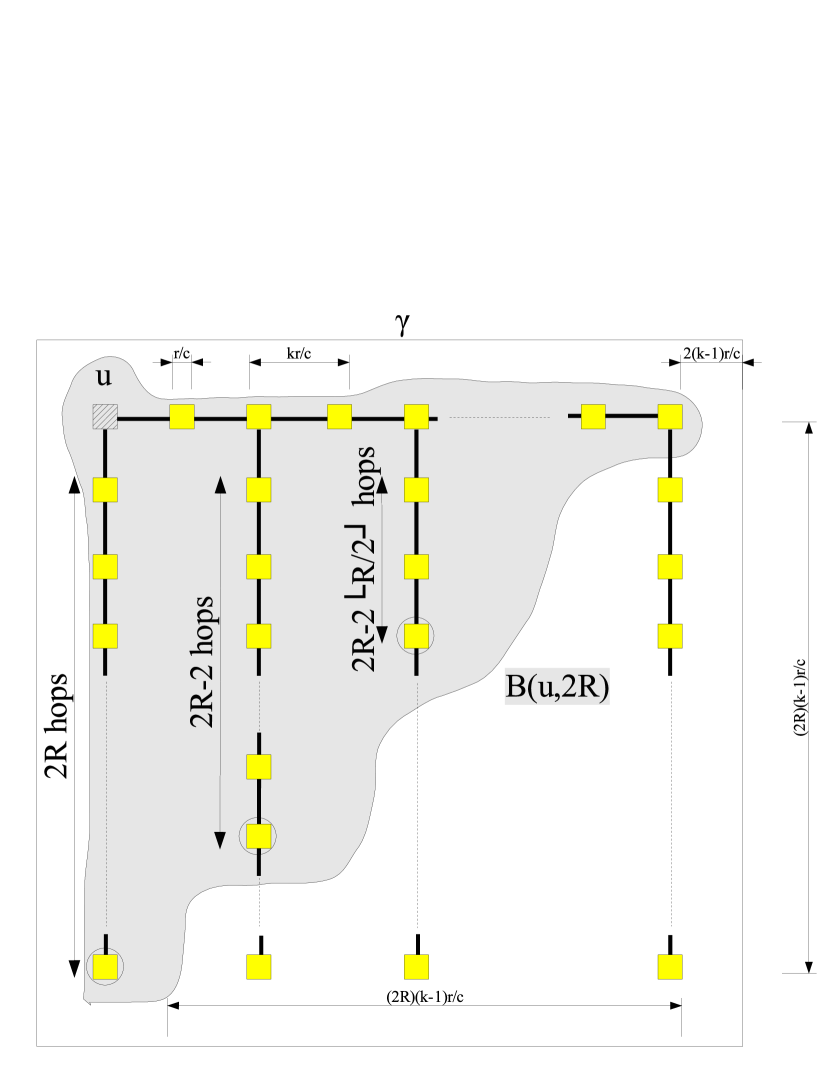
Figure 19: Graph for the proof of lemma 1

Consider the small square shown in Fig. 19 of side $\gamma r$, where $\gamma$ is a constant independent of $n$ to be specified later. Subdivide the small square further into mini-squares of side $r/c$. Choose the constant $c$ such that there exists a constant $k$ satisfying $\sqrt{2}(k-2)>c\geq\sqrt{k^{2}+1}$. Under these conditions, two nodes in mini-squares separated by $(k-2)$ other mini-square will be connected, but not mini-squares $r(k-2)\sqrt{2}/c$ apart (see right hand side of Fig. 19). Consider now the graph on the left hand side of Fig. 19. Assume that each full (colored) mini-square contains exactly one node. We now focus on the ball $\mathcal{B}_{2R}^{\mathcal{G}}(u)$ and will lower bound the number of balls of radius $R$ necessary to cover it. On the $\left\lfloor R/2\right\rfloor$ first vertical branches from the left, the last node of the branch inside that ball (circled) must be covered by a ball of radius $R$ centered on the same branch. This is clear since the length of the branch is larger than $R$. Consequently, the doubling dimension of this graph is at least $\mbox{$\left\lfloor R/2\right\rfloor$}\geq\frac{R-1}{2}$. We want the doubling dimension to be larger than $\beta$, which can be easily achieved by choosing $R$ such that $\frac{R-1}{2}>\beta$. Let $R=2\beta+2>2\beta+1$. Further, we can now set $\gamma=(2R+5)(k-1)/c=(4\beta+9)(k-1)/c$ and $b=(2R+1)\mbox{$\left\lceil\frac{2R+1}{2}+1\right\rceil$}=(4\beta+5)\mbox{$\left\lceil\frac{4\beta+5}{2}+1\right\rceil$}$. This ensures that the doubling dimension is strictly larger than $\beta$.

It remains to be shown that when such a small square contains $b$ nodes, the graph constructed above occurs with probability $p>0$. The number $m$ of mini-squares contained in a small square of side $\gamma r$ is $m=\frac{\gamma^{2}r^{2}}{r^{2}/c^{2}}=\gamma^{2}c^{2}$ which is constant. Each node can fall in any of the $m$ squares with equal probability. Hence, all $m^{b}$ configurations are equiprobable and $p=\frac{1}{m^{b}}>0$. ∎

We number the small squares from $1$ to $m=\frac{n}{(\gamma r)^{2}}=\frac{n}{\gamma^{2}\log^{1-\theta}{n}}$ and denote by $X_{i}^{b}$ the indicator variable that takes value $1$ when small square $i$ contains exactly $b$ nodes.

Lemma 2

There are at least $n^{1/2}$ squares containing $b$ nodes with probability at least $(1-O(\frac{1}{e^{n^{0.25}}}))$ for n sufficiently large

Proof:

$$\begin{array}[]{ll}\mbox{$\mathcal{E}\left[X\right]$}&=\mbox{$\mathcal{E}\left[\sum_{i=1}^{m}X_{i}^{b}\right]$}\\ &=\sum_{i=1}^{m}\mbox{$\mathcal{P}\left[X_{i}^{b}\right]$}\\ &=\sum_{i=1}^{m}{n\choose b}(\frac{1}{m})^{b}(1-\frac{1}{m})^{n-b}\\ &\geq m(\frac{n}{b})^{b}(\frac{1}{m})^{b}(1-\frac{1}{m})^{n}\\ &\geq\frac{n}{b^{b}}(\gamma^{2}\log^{1-\theta}{n})^{b-1}(1-\frac{1}{m})^{m\gamma^{2}\log^{1-\theta}{n}}\\ &\geq\frac{n}{b^{b}}(\gamma^{2}\log^{1-\theta}{n})^{b-1}\frac{1}{2^{2\gamma^{2}\log_{2}^{1-\theta}{n}/\log_{2}^{1-\theta}{e}}}\\ &\geq O(n^{1-O(\frac{1}{\log^{\theta}{n}})})\\ &\geq O(n^{\delta})\end{array}$$

where $\delta\geq\frac{7}{8}$ for $n$ sufficiently large, since $\theta>\zeta$.

Let $S_{i}$ be the random variable representing the small square into which the $i^{th}$ node falls. Let $F$ be the number of small squares containing exactly $b$ nodes after all nodes have been placed. Then the sequence $Z_{i}=\mbox{$\mathcal{E}\left[F|S_{1},...,S_{i}\right]$}$ is a Doob Martingale. One can show that $F=f(S_{1},S_{2},...,S_{n})$ satisfies the Lipschitz condition with bound $1$. Indeed, changing the placement of the $i^{th}$ ball can only modify the value of $F$ by at most $1$. We therefore obtain:

$$\mbox{$\mathcal{P}\left[|F-\mbox{$\mathcal{E}\left[F\right]$}|\geq n^{5/8}\right]$}\leq 2e^{-2n^{10/8-1}}=2\frac{1}{e^{2n^{1/4}}}$$

by the Azuma-Hoeffding inequality. Consequently,

$$\begin{array}[]{ll}\mbox{$\mathcal{P}\left[F<n^{1/2}\right]$}&<\mbox{$\mathcal{P}\left[F<\underbrace{\mbox{$\mathcal{E}\left[F\right]$}-n^{5/8}}_{=n^{7/8}-n^{5/8}>n^{1/2}}\right]$}\\ &\leq 2\frac{1}{e^{2n^{1/4}}}\leq 2\frac{1}{e^{n^{1/4}}}\end{array}$$

and

$$\mbox{$\mathcal{P}\left[F\geq n^{1/2}\right]$}\geq(1-2\frac{1}{e^{n^{1/4}}})$$

∎

It now remains to show that in this regime, $\mathcal{G}(n,r)$ are not doubling with high probability.

Theorem 17

$\mathcal{G}(n,(\log{n})^{\frac{1}{2}-\frac{\theta}{2}})$, where $\theta\in\left.\right]\zeta,1\left[\right.$ and $\zeta$ is a constant such that $0<\zeta<1$, are not doubling with high probability.

Proof:

By Lemma 1, for any constant $\beta$, a small square area of side $\gamma r$ with $b$ nodes contains a graph of doubling dimension $>\beta$ with probability $p>0$. By Lemma 2, there are $n^{1/2}$ such small squares containing $b$ nodes w.h.p. Let $F$ denote the number of small squares containing exactly $b$ nodes. Consequently, the probability that at least one of this squares contains a graph of doubling dimension $>\beta$ is given by:

$$\begin{array}[]{ll}\mbox{$\mathcal{P}\left[\mbox{not doubling}\right]$}&=\sum_{j=1}^{m}\mbox{$\mathcal{P}\left[\mbox{not doubling}|F=j\right]$}\mbox{$\mathcal{P}\left[F=j\right]$}\\ &\geq(1-O(\frac{1}{e^{n^{0.25}}}))\sum_{j=n^{1/2}}^{m}(1-(1-p)^{j})\\ &\geq(1-(1-p)^{n^{1/2}})(1-O(\frac{1}{e^{n^{0.25}}}))\\ &\geq(1-(1-p)^{n^{1/2}})^{2}\\ &\geq(1-\frac{2}{x^{O(n)}})\end{array}$$

where $x=(\frac{1}{1-p})>1$. Consequently, with probability at least $(1-\frac{2}{x^{O(n)}})$, there exists no constant which bounds the doubling dimension of $\mathcal{G}(n,(\log{n})^{\frac{1}{2}-\frac{\theta}{2}})$. ∎

References

- [AGGM06] I. Abraham, C. Gavoille, A. V. Goldberg, and D. Malkhi, Routing in networks with low doubling dimension, ICDCS, 2006.
- [BV05] J.-Y. Le Boudec and M. Vojnovic, Perfect simulation and stationarity of a class of mobility models, INFOCOM, 2005.
- [CGMZ05] T-H. Hubert Chan, Anupam Gupta, Bruce M. Maggs, and Shuheng Zhou, On hierarchical routing in doubling metrics, SODA, 2005.
- [FRZ+05] Rodrigo Fonseca, Sylvia Ratnasamy, Jerry Zhao, Cheng Tien Ee, David Culler, Scott Shenker, and Ion and Stoica, Beacon-vector routing: Scalable point-to-point routing in wireless sensor networks, NSDI, 2005.
- [Gav01] C. Gavoille, Routing in distributed networks, ACM SIGACT News (2001), 36.
- [GK98] P. Gupta and P. R. Kumar, Critical power for asymptotic connectivity in wireless networks, Stochastic Analysis, Control, Optimization and Applications (1998).
- [GK00] P. Gupta and P. R. Kumar, The capacity of wireless networks, IEEE Transactions on Information Theory 46 (2000), no. 2, 388–404.
- [JMB01] D. B. Johnson, D. A. Maltz, and J. Broch, Dsr: The dynamic source routing protocol for multi-hop wireless ad hoc networks, Ad Hoc Networking (Addison-Wesley Longman Publishing Co., ed.), 2001, Book, p. 139 172.
- [KK00] Brad Karp and H. T. Kung, Gpsr: Greedy perimeter stateless routing for wireless networks, MOBICOM, 2000, p. 243.
- [KRX06] Goran Konjevod, Andrea W. Richa, and Donglin Xia, Optimal stretch name independent compact routing in doubling metrics, PODC, 2006.
- [KV02] S. R. Kulkarni and P. Viswanath, A deterministic approach to throughput scaling in wireless networks, ISIT, 2002, p. 351.
- [LJDC+00] Jinyang Li, John Jannotti, Douglas S. J. De Couto, David R. Karger, and Robert Morris, Scalable location service for geographic ad hoc routing, MOBICOM, 2000, p. 120.
- [MSZ06] Eytan Modiano, Devavrat Shah, and Gil Zussman, Maximizing throughput in wireless networks via gossip, ACM SIGMETRIC’06, 2006, p. 26.
- [PR97] C. Perkins and E. M. Royer, Ad-hoc on-demand distance vector routing, MILCOM ’97 panel on Ad Hoc Networks, 1997.
- [RRP+03] A. Rao, S. Ratnasamy, C. Papadimitriou, S. Shenker, and I. Stoica, Geographic routing without location information, MOBICOM, 2003, p. 96.
- [RS98] Martin Raab and Angelika Steger, Balls into bins: A simple and tight analysis, Lecture Notes in Computer Science 1518 (1998), 159.
- [SMS06] G. Sharma, R. Mazumdar, and N. Shroff, Delay and capacity trade-offs in mobile ad hoc networks: A global perspective, INFOCOM, 2006, p. 1.
- [Tal04] Kunal Talwar, Bypassing the embedding: algorithms for low dimensional metrics, STOC (Chicago, IL, USA), 2004, p. 281.
- [TDGW07] D. Tschopp, S. Diggavi, M. Grossglauser, and J. Widmer, Robust geo-routing on embeddings of dynamic wireless networks, INFOCOM, 2007, p. 1730.