Entanglement transfer through the turbulent atmosphere

Abstract

The propagation of polarization-entangled states of light through fluctuating loss channels in the turbulent atmosphere is studied, including the situation of strong losses. We consider violations of Bell inequalities by light, emitted by a parametric down-conversion source, after transmission through the turbulent atmosphere. It is shown by analytical calculations, that in the presence of background radiation and dark counts, fluctuating loss channels may preserve entanglement properties of light even better than standard loss channels, when postselected measurements are applied.

I Introduction

The distribution of quantum light through the turbulent atmosphere has attracted a great deal of attention since recent experiments Fedrizzi ; Ursin ; QKD ; Elser have demonstrated the feasibility of quantum key distribution in free-space channels. In this connection the question arises as to whether nonclassical properties of light can be preserved during its propagation in fluctuating media. Particularly, special interest is applied to the transfer of entanglement Horodecki through the turbulent atmosphere since this problem has important perspectives in quantum communications.

The theory of classical light distributed through the atmosphere was established many years ago Tatarskii-Fante . Phenomena such as beam wander, scintillations, beam spreading, and spatial coherence degradation have been explained in the framework of this description. It is based on Kolmogorov’s theory of turbulence, which is successfully applied to a description of wave propagation in random media.

The theory of nonclassical phenomena, such as entanglement, for light propagation in random media is less developed. First, one should mention the approach proposed in Ref. DiamentPerinaMilonni for the description of the photocounting statistics of quantum light propagating through the turbulent atmosphere. The idea of this approach is based on the introduction of a stochastic intensity modulation for light propagating through random media. Another approach describing nonclassical properties of light is based on the photon wave function Paterson . It enables one to describe a special class of entangled states of light in the turbulent atmosphere Smith . The concept of the single-photon wave function can be formulated in a more sophisticated way in terms of the single-photon Wigner function and then generalized to the description of arbitrary quantum states. This technique has been developed in Chumak and applied to some interesting examples of quantum and classical light.

Recently, a theoretical model for the light distributed through the turbulent atmosphere and processed by homodyne detection has been proposed Semenov1 . The idea is based on the description of random media in terms of a fluctuating loss channel. It has been shown that the turbulent atmosphere introduces, compared with standard loss channels, additional noise into quantum states of light. The presence of such noise has also been discussed recently in Ref. Marquardt . Moreover, as has been shown in Ref. Semenov1 , the nonclassicality of bright light fields (especially fields with a large coherent amplitude) is more fragile against turbulence than the nonclassicality of weak light. In this connection special interest should be paid to entangled photon pairs and single photons, whose fields are weak enough to preserve their nonclassical properties.

In this paper we give a systematic theoretical description of polarization-entangled states of light distributed through the fluctuating loss channels in the atmosphere and processed by polarization analyzers. For such light we check violations of Bell inequalities Bell ; CHSH . Besides turbulence our consideration includes imperfect detection and noise counts originating from internal dark counts and background radiation. Moreover, we deal with a realistic parametric down-conversion (PDC) source of the radiation Fedrizzi ; Ursin ; PDC . We apply the results of our consideration to analyzing a recently reported experiment Fedrizzi , where light has been distributed over a 144-km atmospheric channel between two Canary Islands in a configuration with both receivers being co-located at the same place. We show that with fluctuating loss channels one may observe larger values of the Bell parameter compared with corresponding nonfluctuating loss channels. This unexpected effect is caused by those (postselected) random events which are related to small losses.

The paper is organized as follows. In Sec. II we summarize the needed basic principles of Bell-type experiments. A systematic description of fluctuating loss channels for the case of such experiments is given in Sec. III. In Sec. IV we consider the violation of Bell inequalities by light after propagation through the turbulent atmosphere, when the source generates perfect Bell states. The situation for a realistic PDC source is analyzed in Sec. V. In Sec. VI we describe a procedure for measuring the needed turbulence parameters. A summary and some concluding remarks are given in Sec. VII.

II Bell-type experiments

Let us start with the consideration of a typical experimental setup (see Fig. 1). The entangled photon pairs are emitted by the source $S$ and then transferred through the turbulent atmosphere to the receiver stations $A$ and $B$. In principle, different configurations of the considered experiment are possible: The source can be placed separately from both receivers (e.g., on a low-orbit satellite), it can be placed on the site of one of the receivers Ursin , or both receivers can be situated at the same place Fedrizzi (a configuration convenient for testing the feasibility of entanglement transfer). At the receiver stations the light is collected by a telescope (or other device) and subsequently directed to the polarization analyzers. Each of these analyzers consists of a half-wave plate (which turns the polarization direction by the angles $\theta_{\mathrm{A}}$ and $\theta_{\mathrm{B}}$ at the receiver stations $A$ and $B$, respectively), a polarizing beam-splitter, and two detectors.

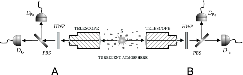
Figure 1: A typical experimental setup for checking the violation of Bell inequalities for light transmitting through turbulent atmosphere. The source $S$ produces entangled photon pairs. The polarization analyzers at $\mathrm{A}$ and $\mathrm{B}$ sites consist of half-wave plates, $HWP$, polarizer beam-splitters, $PBS$, and two pairs of detectors: $D_{\mathrm{T_{A}}}$ for the transmitted signal and $D_{\mathrm{R_{A}}}$ for the reflected signal at the $A$ site; $D_{\mathrm{T_{B}}}$ for the transmitted signal and $D_{\mathrm{R_{B}}}$ for the reflected signal at the $B$ site.

According to photodetection theory PhotoDetection ; MandelBook , the probability of registering one count at the detector $i_{\mathrm{A}}=\{\mathrm{T_{A}},\mathrm{R_{A}}\}$ by receiver $A$, one count at the detector $i_{\mathrm{B}}=\{\mathrm{T_{B}},\mathrm{R_{B}}\}$ by receiver $B$, and no counts at the other detectors is given by

$$P_{\mathrm{i_{\mathrm{A}},i_{\mathrm{B}}}}\left(\theta_{\mathrm{A}},\theta_{\mathrm{B}}\right)=\mbox{\rm Tr}\left(\hat{\Pi}_{i_{\mathrm{A}}}^{(1)}\hat{\Pi}_{i_{\mathrm{B}}}^{(1)}\hat{\Pi}_{j_{\mathrm{A}}}^{(0)}\hat{\Pi}_{j_{\mathrm{B}}}^{(0)}\hat{\varrho}\right),$$ (1)

$i_{\mathrm{A}}\neq j_{\mathrm{A}}$, $i_{\mathrm{B}}\neq j_{\mathrm{B}}$, where $\hat{\varrho}$ is the density operator of the light field at the inputs of both polarization analyzers,

$$\hat{\Pi}_{i_{\mathrm{A(B)}}}^{(n)}=:\frac{\left(\eta_{i_{\mathrm{A(B)}}}\!\hat{n}_{i_{\mathrm{A(B)}}}+N_{i_{\mathrm{A(B)}}}\right)^{n}}{n!}e^{-\eta_{i_{\mathrm{A(B)}}}\!\hat{n}_{i_{\mathrm{A(B)}}}-N_{i_{\mathrm{A(B)}}}}:$$ (2)

is the positive operator-valued measure for the detector $i_{\mathrm{A(B)}}$ Semenov3 , $\eta_{i_{\mathrm{A(B)}}}$ and $N_{i_{\mathrm{A(B)}}}$ are the efficiency and the mean value of noise counts (originating from internal dark counts and background radiation), respectively, for the detector $i_{\mathrm{A(B)}}$, and $:\hskip 5.0pt:$ means normal ordering. The photon number operator at the input of the detector $i_{\mathrm{A(B)}}$ can be written in terms of the corresponding annihilation and creation operators,

$$\hat{n}_{i_{\mathrm{A(B)}}}=\hat{a}^{\dagger}_{i_{\mathrm{A(B)}}}\hat{a}_{i_{\mathrm{A(B)}}}.$$ (3)

These operators can be expressed via the operators of the horizontal and vertical modes, $\hat{a}_{\scriptscriptstyle\mathrm{H_{A(B)}}}$ and $\hat{a}_{\scriptscriptstyle\mathrm{V_{A(B)}}}$, respectively, at the input of the polarization analyzers as

$$\hat{a}_{\scriptscriptstyle T_{\mathrm{A(B)}}}=\hat{a}_{\scriptscriptstyle\mathrm{H_{A(B)}}}\cos\theta_{\mathrm{A(B)}}+\hat{a}_{\scriptscriptstyle\mathrm{V_{A(B)}}}\sin\theta_{\mathrm{A(B)}},$$ (4)

$$\hat{a}_{\scriptscriptstyle R_{\mathrm{A(B)}}}=-\hat{a}_{\scriptscriptstyle\mathrm{H_{A(B)}}}\sin\theta_{\mathrm{A(B)}}+\hat{a}_{\scriptscriptstyle\mathrm{V_{A(B)}}}\cos\theta_{\mathrm{A(B)}}.$$ (5)

In the case of using on/off detectors, which cannot distinguish between different photon numbers, Eq. (1) should be rewritten as

$$P_{\mathrm{i_{\mathrm{A}},i_{\mathrm{B}}}}\left(\theta_{\mathrm{A}},\theta_{\mathrm{B}}\right)=\sum\limits_{n,m=1}^{+\infty}\mbox{\rm Tr}\left(\hat{\Pi}_{i_{\mathrm{A}}}^{(n)}\hat{\Pi}_{i_{\mathrm{B}}}^{(m)}\hat{\Pi}_{j_{\mathrm{A}}}^{(0)}\hat{\Pi}_{j_{\mathrm{B}}}^{(0)}\hat{\varrho}\right).$$ (6)

The correlation coefficient, which appears in the Bell theory Bell , is given by

$$E\left(\theta_{\mathrm{A}},\theta_{\mathrm{B}}\right)=\frac{P_{\mathrm{same}}\left(\theta_{\mathrm{A}},\theta_{\mathrm{B}}\right)-P_{\mathrm{different}}\left(\theta_{\mathrm{A}},\theta_{\mathrm{B}}\right)}{P_{\mathrm{same}}\left(\theta_{\mathrm{A}},\theta_{\mathrm{B}}\right)+P_{\mathrm{different}}\left(\theta_{\mathrm{A}},\theta_{\mathrm{B}}\right)},$$ (7)

where

$$P_{\mathrm{same}}\left(\theta_{\mathrm{A}},\theta_{\mathrm{B}}\right)=P_{\mathrm{\mathrm{T_{A}},\mathrm{T_{B}}}}\left(\theta_{\mathrm{A}},\theta_{\mathrm{B}}\right)+P_{\mathrm{\mathrm{R_{A}},\mathrm{R_{B}}}}\left(\theta_{\mathrm{A}},\theta_{\mathrm{B}}\right)$$ (8)

is the probability of getting clicks on both detectors in the transmission channels or both detectors in the reflection channels, and

$$P_{\mathrm{different}}\left(\theta_{\mathrm{A}},\theta_{\mathrm{B}}\right)=P_{\mathrm{\mathrm{T_{A}},\mathrm{R_{B}}}}\left(\theta_{\mathrm{A}},\theta_{\mathrm{B}}\right)+P_{\mathrm{\mathrm{R_{A}},\mathrm{T_{B}}}}\left(\theta_{\mathrm{A}},\theta_{\mathrm{B}}\right)$$ (9)

is the probability to get clicks on the detectors in the transmission channel at one site and the reflection channel at another site. According to the Clauser-Horne-Shimony-Holt (CHSH) Bell-type inequality CHSH for any local-realistic theory the maximal value of the parameter

$$\mathcal{B} = \left|E\left(\theta_{\mathrm{A}}^{(1)},\theta_{\mathrm{B}}^{(1)}\right)-E\left(\theta_{\mathrm{A}}^{(1)},\theta_{\mathrm{B}}^{(2)}\right)\right|$$

$$+ \left|E\left(\theta_{\mathrm{A}}^{(2)},\theta_{\mathrm{B}}^{(2)}\right)+E\left(\theta_{\mathrm{A}}^{(2)},\theta_{\mathrm{B}}^{(1)}\right)\right|,$$

should be

$$\mathcal{B}\leq 2.$$ (11)

Quantum light may violate this inequality. In this case the maximal violating by the value $2\sqrt{2}$ is reached for the Bell state

$$\left|\mathrm{\mathcal{B}}\right\rangle = \frac{1}{\sqrt{2}}\Big{(}\left|\mathrm{1}\right\rangle_{\mathrm{H_{A}}}\left|\mathrm{0}\right\rangle_{\mathrm{V_{A}}}\left|\mathrm{0}\right\rangle_{\mathrm{H_{B}}}\left|\mathrm{1}\right\rangle_{\mathrm{V_{B}}}\Big{.}$$ (12)

. $$+ e^{i\varphi}\left|\mathrm{0}\right\rangle_{\mathrm{H_{A}}}\left|\mathrm{1}\right\rangle_{\mathrm{V_{A}}}\left|\mathrm{1}\right\rangle_{\mathrm{H_{B}}}\left|\mathrm{0}\right\rangle_{\mathrm{V_{B}}}\Big{)}$$

$$\equiv \frac{1}{\sqrt{2}}\Big{(}\left|\mathrm{\mathrm{H}}\right\rangle_{\mathrm{A}}\left|\mathrm{\mathrm{V}}\right\rangle_{\mathrm{B}}+e^{i\varphi}\left|\mathrm{\mathrm{V}}\right\rangle_{\mathrm{A}}\left|\mathrm{\mathrm{H}}\right\rangle_{\mathrm{B}}\Big{)},$$

for $\varphi=\pi$ and $\big{(}\theta_{\mathrm{A}}^{(1)},\theta_{\mathrm{B}}^{(1)},\theta_{\mathrm{A}}^{(2)},\theta_{\mathrm{B}}^{(2)}\big{)}=\big{(}0,\frac{\pi}{8},\frac{\pi}{4},\frac{3\pi}{8}\big{)}$.

III Fluctuating loss channels

The next problem is to derive the density operator $\hat{\varrho}$ for the light transmitted through the turbulent atmosphere. Similar to Ref. Semenov1 , where homodyne detection of such light has been studied, we will consider the atmosphere as an attenuating system. However, an important feature of the present case is that the nonmonochromatic output mode is not specified by the local oscillator; it can take an arbitrary form depending on the distribution of the refraction index in space. Generally speaking, it is impossible to describe such light in terms of a monochromatic or nonmonochromatic four-mode density operator. However, it can be represented in terms of four nonmonochromatic modes with fluctuating shapes. Of course, such a representation is rather formal since it is difficult to provide phase-sensitive measurements for such a mode. However, it appears to be useful for evaluating observable quantities in the considered experiment.

Let $\hat{a}^{\mathrm{in}}_{\scriptscriptstyle\mathrm{H_{A(B)}}}$ and $\hat{a}^{\mathrm{in}}_{\scriptscriptstyle\mathrm{V_{A(B)}}}$ be the field annihilation operators of the horizontal and vertical modes, respectively, generated by the source in the direction of the $A(B)$ receiver station. The operator input–output relations for the attenuating system can be written as

$$\hat{a}_{\scriptscriptstyle\mathrm{H_{A(B)}}}=T_{\mathrm{H_{A(B)}}}\hat{a}^{\mathrm{in}}_{\scriptscriptstyle\mathrm{H_{A(B)}}}+T_{\mathrm{HV_{A(B)}}}\hat{a}^{\mathrm{in}}_{\scriptscriptstyle\mathrm{V_{A(B)}}}+R_{\mathrm{H_{A(B)}}}\hat{c}^{\mathrm{in}}_{\scriptscriptstyle\mathrm{H_{A(B)}}},$$

(13)

$$\hat{a}_{\scriptscriptstyle\mathrm{V_{A(B)}}}=T_{\mathrm{V_{A(B)}}}\hat{a}^{\mathrm{in}}_{\scriptscriptstyle\mathrm{V_{A(B)}}}+T_{\mathrm{VH_{A(B)}}}\hat{a}^{\mathrm{in}}_{\scriptscriptstyle\mathrm{H_{A(B)}}}+R_{\mathrm{V_{A(B)}}}\hat{c}^{\mathrm{in}}_{\scriptscriptstyle\mathrm{V_{A(B)}}},$$

(14)

where $T_{\mathrm{H_{A(B)}}}$ and $T_{\mathrm{V_{A(B)}}}$ are the transmission coefficients for the horizontal and vertical modes, respectively, in the direction of the $A(B)$ receiver stations; $\hat{c}^{\mathrm{in}}_{\scriptscriptstyle\mathrm{H_{A(B)}}}$ and $\hat{c}^{\mathrm{in}}_{\scriptscriptstyle\mathrm{V_{A(B)}}}$ are the operators describing the losses related to absorption and scattering with the absorption and reflection coefficients $R_{\mathrm{H_{A(B)}}}$ and $R_{\mathrm{V_{A(B)}}}$, respectively. Since the depolarization effect of the atmosphere is extremely small Tatarskii-Fante , we may set in the following $T_{\mathrm{HV_{A(B)}}}\approx 0$, $T_{\mathrm{VH_{A(B)}}}\approx 0$, and $T_{\mathrm{H_{A(B)}}}\approx T_{\mathrm{V_{A(B)}}}\equiv T_{\mathrm{A(B)}}$. Hence, the operator input–output relations (13) and (14) can be simply written as

$$\hat{a}_{\scriptscriptstyle\mathrm{H_{A(B)}}}=T_{\mathrm{A(B)}}\hat{a}^{\mathrm{in}}_{\scriptscriptstyle\mathrm{H_{A(B)}}}+R_{\mathrm{H_{A(B)}}}\hat{c}^{\mathrm{in}}_{\scriptscriptstyle\mathrm{H_{A(B)}}},$$ (15)

$$\hat{a}_{\scriptscriptstyle\mathrm{V_{A(B)}}}=T_{\mathrm{A(B)}}\hat{a}^{\mathrm{in}}_{\scriptscriptstyle\mathrm{V_{A(B)}}}+R_{\mathrm{V_{A(B)}}}\hat{c}^{\mathrm{in}}_{\scriptscriptstyle\mathrm{V_{A(B)}}}.$$ (16)

The transmission coefficients $T_{\mathrm{A(B)}}$ and the absorption and reflection coefficients $R_{\mathrm{{H(V)}_{A(B)}}}$ satisfy the constraints

$$\left|T_{\mathrm{A(B)}}\right|^{2}+\left|R_{\mathrm{{H(V)}_{A(B)}}}\right|^{2}=1,$$ (17)

These relations can be converted into the corresponding relations between the density operator $\hat{\varrho}_{\mathrm{in}}$ of the light generated by the source and the density operator $\hat{\varrho}_{\bf\scriptscriptstyle T}$ [where ${\bf T}=\left(T_{\mathrm{A}},T_{\mathrm{B}}\right)$] of the light transmitted through the loss channels under the assumption that the absorption and scattering system is in the vacuum state. For example, the relation between the Glauber-Sudarshan $P$ function GlauberSudarshan of the attenuated light, $P_{\bf\scriptscriptstyle T}\left(\alpha_{\mathrm{\scriptscriptstyle H_{A}}},\alpha_{\mathrm{\scriptscriptstyle V_{A}}},\alpha_{\mathrm{\scriptscriptstyle H_{B}}},\alpha_{\mathrm{\scriptscriptstyle V_{B}}}\right)$, and the $P$ function of the light generated by the source, $P_{\mathrm{in}}\left(\alpha_{\mathrm{\scriptscriptstyle H_{A}}},\alpha_{\mathrm{\scriptscriptstyle V_{A}}},\alpha_{\mathrm{\scriptscriptstyle H_{B}}},\alpha_{\mathrm{\scriptscriptstyle V_{B}}}\right)$, is given by MandelBook

$$P_{\bf\scriptscriptstyle T}\left(\alpha_{\mathrm{\scriptscriptstyle H_{A}}},\alpha_{\mathrm{\scriptscriptstyle V_{A}}},\alpha_{\mathrm{\scriptscriptstyle H_{B}}},\alpha_{\mathrm{\scriptscriptstyle V_{B}}}\right)$$

$$=\frac{1}{\left|T_{\mathrm{A}}\right|^{4}\left|T_{\mathrm{B}}\right|^{4}}P_{\mathrm{in}}\left(\frac{\alpha_{\mathrm{\scriptscriptstyle H_{A}}}}{T_{\mathrm{A}}},\frac{\alpha_{\mathrm{\scriptscriptstyle V_{A}}}}{T_{\mathrm{A}}},\frac{\alpha_{\mathrm{\scriptscriptstyle H_{B}}}}{T_{\mathrm{B}}},\frac{\alpha_{\mathrm{\scriptscriptstyle V_{B}}}}{T_{\mathrm{B}}}\right).$$ (18)

Similarly, the corresponding characteristic function of the attenuated light, $\Phi_{\bf\scriptscriptstyle T}\left(\beta_{\mathrm{\scriptscriptstyle H_{A}}},\beta_{\mathrm{\scriptscriptstyle V_{A}}},\beta_{\mathrm{\scriptscriptstyle H_{B}}},\beta_{\mathrm{\scriptscriptstyle V_{B}}}\right)$, is related to the characteristic function of the light generated by the source, $\Phi_{\mathrm{in}}\left(\beta_{\mathrm{\scriptscriptstyle H_{A}}},\beta_{\mathrm{\scriptscriptstyle V_{A}}},\beta_{\mathrm{\scriptscriptstyle H_{B}}},\beta_{\mathrm{\scriptscriptstyle V_{B}}}\right)$, as

$$\Phi_{\bf\scriptscriptstyle T}\left(\beta_{\mathrm{\scriptscriptstyle H_{A}}},\beta_{\mathrm{\scriptscriptstyle V_{A}}},\beta_{\mathrm{\scriptscriptstyle H_{B}}},\beta_{\mathrm{\scriptscriptstyle V_{B}}}\right)$$ (19)

$$=\Phi_{\mathrm{in}}\left(T^{\ast}_{\mathrm{A}}\beta_{\mathrm{\scriptscriptstyle H_{A}}},T^{\ast}_{\mathrm{A}}\beta_{\mathrm{\scriptscriptstyle V_{A}}},T^{\ast}_{\mathrm{B}}\beta_{\mathrm{\scriptscriptstyle H_{B}}},T^{\ast}_{\mathrm{B}}\beta_{\mathrm{\scriptscriptstyle V_{B}}}\right).$$

The corresponding expressions can also be written for $s$-parametrized phase-space distribution, for normal-ordered moments (see, e.g., Ref. Semenov1 ), for the density operator in the Fock-state representation FockStateEff , and, in principle for an arbitrary representation of the density operator.

The main difference of the fluctuating loss channels from the standard loss channels is that the transmission coefficients $T_{\mathrm{A}}$ and $T_{\mathrm{B}}$ are random variables. This means that the density operator of the field at the input of the polarization analyzers, $\hat{\varrho}$, should be obtained by averaging the density operator $\hat{\varrho}_{\bf\scriptscriptstyle T}$ with the probability distribution of the transmission coefficient (PDTC), $\mathcal{P}\left({\mathbf{T}}\right)$,

$$\hat{\varrho}=\int\limits_{\mathrm{D}}\mathbf{dT}\,\mathcal{P}\left({\mathbf{T}}\right)\,\hat{\varrho}_{\bf\scriptscriptstyle T},$$ (20)

where $\mathbf{dT}=d^{2}T_{\mathrm{A}}\,d^{2}T_{\mathrm{B}}$, and the integration domain is defined by the conditions

$$\mathrm{D}=\left\{\left|T_{\mathrm{A}}\right|^{2}\leq 1,\,\left|T_{\mathrm{B}}\right|^{2}\leq 1\right\}.$$ (21)

Such an approach is closely related to the idea of a random intensity modulation in the description of the photocounting distribution for light transmitted through turbulent media DiamentPerinaMilonni . An important difference is that the factor of the intensity modulation was allowed to attain values in the range of $\left[0,+\infty\right)$. In our approach this domain is restricted to $\left[0,1\right]$, which preserves the required positivity of the density operator in Eq. (20).

IV Bell States

We start with the consideration of the idealized situation, when the source generates the Bell state (12). This will help us to better understand the nature of contributions from noise, atmospheric turbulence, and different experimental imperfections. First, we consider the density operator (and its entanglement properties) of such a state after passing the light through fluctuating loss channels. Next, we include in the consideration background radiation, dark counts, and detection losses – for such conditions we analyze violations of Bell inequalities.

IV.1 Output density operator

The density operator of the Bell state (12) is simply written as $\hat{\varrho}_{\mathrm{in}}=\hat{\varrho}_{\mathcal{\scriptscriptstyle B}}\equiv\left|\mathrm{\mathcal{B}}\right\rangle\left\langle\mathrm{\mathcal{B}}\right|$. Utilizing Eqs. (18)-(20) one gets that the corresponding density operator for the light at the input ports of the polarization analyzers is written as a convex combination,

$$\hat{\varrho}=p_{\scriptscriptstyle\mathrm{0}}\hat{\varrho}_{\scriptscriptstyle\mathrm{0}}+p_{\scriptscriptstyle\mathrm{H_{A}}}\hat{\varrho}_{\scriptscriptstyle\mathrm{H_{A}}}+p_{\scriptscriptstyle\mathrm{V_{A}}}\hat{\varrho}_{\scriptscriptstyle\mathrm{V_{A}}}+p_{\scriptscriptstyle\mathrm{H_{B}}}\hat{\varrho}_{\scriptscriptstyle\mathrm{H_{B}}}+p_{\scriptscriptstyle\mathrm{V_{B}}}\hat{\varrho}_{\scriptscriptstyle\mathrm{V_{B}}}+p_{\mathcal{\scriptscriptstyle B}}\hat{\varrho}_{\mathcal{\scriptscriptstyle B}},$$ (22)

of the following states: vacuum state $\hat{\varrho}_{\scriptscriptstyle\mathrm{0}}$ with the probability

$$p_{\scriptscriptstyle\mathrm{0}}=\left\langle\left(1-\left|T_{\mathrm{A}}\right|^{2}\right)\left(1-\left|T_{\mathrm{B}}\right|^{2}\right)\right\rangle\Big{.}$$ (23)

single-photon states $\hat{\varrho}_{\scriptscriptstyle\mathrm{H_{A}}}$, $\hat{\varrho}_{\scriptscriptstyle\mathrm{V_{A}}}$, $\hat{\varrho}_{\scriptscriptstyle\mathrm{H_{B}}}$, and $\hat{\varrho}_{\scriptscriptstyle\mathrm{V_{B}}}$ in the corresponding modes with the probabilities

$$p_{\scriptscriptstyle\mathrm{H_{A}}}=p_{\scriptscriptstyle\mathrm{V_{A}}}=\frac{1}{2}\left\langle\left|T_{\mathrm{A}}\right|^{2}\left(1-\left|T_{\mathrm{B}}\right|^{2}\right)\right\rangle,$$ (24)

$$p_{\scriptscriptstyle\mathrm{H_{B}}}=p_{\scriptscriptstyle\mathrm{V_{B}}}=\frac{1}{2}\left\langle\left|T_{\mathrm{B}}\right|^{2}\left(1-\left|T_{\mathrm{A}}\right|^{2}\right)\right\rangle,$$ (25)

and the Bell state $\hat{\varrho}_{\scriptscriptstyle\mathcal{B}}$ [cf. Eq. (12)] with the probability

$$p_{\scriptscriptstyle\mathcal{B}}=\left\langle\left|T_{\mathrm{A}}\right|^{2}\left|T_{\mathrm{B}}\right|^{2}\right\rangle.$$ (26)

The brackets $\left\langle\ldots\right\rangle$ mean averaging with the PDTC, $\mathcal{P}\left({\mathbf{T}}\right)$.

In the absence of background radiation and dark counts, only the contribution of the density operator $\hat{\varrho}_{\scriptscriptstyle\mathcal{B}}$ in Eq. (22) is postselected in the measurements. Hence the entanglement properties of the light for such an experiment are not destroyed by the atmospheric turbulence, at least in the absence of dark counts, background noise and other experimental imperfections. The result, nevertheless, may be significantly changed when such effects play a major role.

IV.2 Imperfect photodetection

In the presence of background radiation and dark counts, the postselection procedure no longer results in the perfect separation of the density matrix $\hat{\varrho}^{\scriptscriptstyle\mathcal{B}}$ from the combination (22). Indeed, in this case it is possible that one click at the receiver station $A(B)$ originated from the signal is combined with a click originated from noise at the receiver station $B(A)$. Also it is possible that noise contributes into clicks at both receiver stations.

This situation should be analyzed by substitution of the density operator (22) in Eqs. (1) and (6) and then the result should be used in Eq. (7). The general analytical solution of this problem is given in Appendix A. Here we consider an important special case of equal detectors and equal background noise at all detectors, that is, $\eta_{i_{\mathrm{A(B)}}}=\eta_{\mathrm{c}}$ and $N_{i_{\mathrm{A(B)}}}=N_{\mathrm{nc}}$ for all $i_{\mathrm{A(B)}}$ in Eq. (2).

After some algebra, the correlation coefficient (7) appears to be equal to

$$E\left(\theta_{\mathrm{A}},\theta_{\mathrm{B}}\right)$$ (27)

$$=\mathcal{S}\left[-\cos 2\theta_{\mathrm{A}}\cos 2\theta_{\mathrm{B}}+\cos\varphi\sin 2\theta_{\mathrm{A}}\sin 2\theta_{\mathrm{B}}\right].$$

For photon-number-resolving detectors we get

$$\mathcal{S}=\frac{p_{\scriptscriptstyle\mathcal{B}}\eta_{\mathrm{c}}^{2}}{p_{\scriptscriptstyle\mathcal{B}}\left[\eta_{\mathrm{c}}+2N_{\mathrm{nc}}\left(1-\eta_{\mathrm{c}}\right)\right]^{2}+2p_{\scriptscriptstyle 1}N_{\mathrm{nc}}\left[\eta_{\mathrm{c}}+2N_{\mathrm{nc}}\left(1-\eta_{\mathrm{c}}\right)\right]+4p_{\scriptscriptstyle\mathrm{0}}N_{\mathrm{nc}}^{2}},$$ (28)

and

$$\mathcal{S}=\frac{p_{\scriptscriptstyle\mathcal{B}}\eta_{\mathrm{c}}^{2}e^{2N_{\mathrm{nc}}}}{p_{\scriptscriptstyle\mathcal{B}}\left[\left(1-\eta_{\mathrm{c}}\right)\left(e^{N_{\mathrm{nc}}}-2\right)+e^{N_{\mathrm{nc}}}\right]^{2}+2p_{\scriptscriptstyle 1}\left[e^{N_{\mathrm{nc}}}-1\right]\left[\eta_{\mathrm{c}}e^{N_{\mathrm{nc}}}+2\left(e^{N_{\mathrm{nc}}}-1\right)\left(1-\eta_{\mathrm{c}}\right)\right]+4p_{\scriptscriptstyle\mathrm{0}}\left[e^{N_{\mathrm{nc}}}-1\right]^{2}}$$ (29)

for on/off detectors. Herein, $p_{\scriptscriptstyle 1}=p_{\scriptscriptstyle\mathrm{H_{A}}}+p_{\scriptscriptstyle\mathrm{V_{A}}}+p_{\scriptscriptstyle\mathrm{H_{B}}}+p_{\scriptscriptstyle\mathrm{V_{B}}}$ is the probability of the appearance of a single-photon state.

The visibility $V=E\left(\frac{\pi}{4},\frac{\pi}{4}\right)$ (see Fedrizzi ; Ursin ) can be simply obtained from Eq. (27) as

$$V\left(\varphi\right)=\mathcal{S}\cos\varphi.$$ (30)

The maximal and minimal values for this parameter are $V_{\pm}=\pm\mathcal{S}$. In the case of different detectors and/or different background radiations at these detectors, see Appendix A, we obtain $V_{+}\neq-V_{-}$. The parameter $\mathcal{S}$ strictly depends on both noise counts and turbulence properties of the atmosphere. Hence, in contrast to the case of perfect photodetection, the maximal value of the Bell parameter [Eq. (II)] depends on the atmospheric turbulence. In Fig. 2 we consider this parameter as a function of the parameter $\cos\varphi$, which appears in Eq. (27).

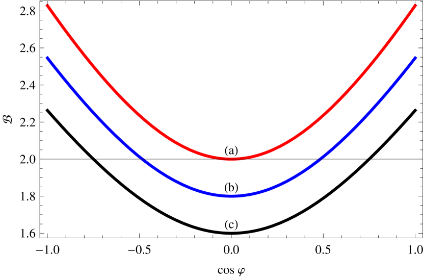
Figure 2: (Color online) The maximal value of the Bell parameter $\mathcal{B}$ vs. $\cos\varphi$, for different values of the parameter $\mathcal{S}$: (a) $1$, (b) $0.9$, (c) $0.8$.

The obtained analytical results can be used for analyzing a realistic experimental situation, such as that considered in Ref. Fedrizzi . In this case both receiver stations had been positioned at the same place. Consequently, the light pulses at receivers $A$ and $B$ have been propagating along the same path through the fluctuating atmosphere. They are separated by a small time interval, which is much less than the characteristic time of the atmospheric fluctuations. Hence, in this case one can simply set

$$\left|T_{\mathrm{A}}\right|^{2}=\left|T_{\mathrm{B}}\right|^{2}\equiv\eta_{\mathrm{atm}},$$ (31)

where $\eta_{\mathrm{atm}}$ is the fluctuating atmospheric efficiency. We also suppose that this efficiency is approximately log-normally distributed Semenov1 ,

$$\mathcal{P}\left(\eta_{\mathrm{atm}}\right)=\frac{1}{\sqrt{2\pi}\sigma\eta_{\mathrm{atm}}}\exp\left[-\frac{1}{2}\left(\frac{\ln\eta_{\mathrm{atm}}+\bar{\theta}}{\sigma}\right)^{2}\right],$$ (32)

where $\bar{\theta}=-\left\langle\ln\eta_{\mathrm{atm}}\right\rangle$ characterizes the mean atmospheric losses and $\sigma$ (the variance of $\theta=-\ln\eta_{\mathrm{atm}}$) characterizes the atmosphere turbulence. It is worth noting that this distribution can be applied only for $\sigma\ll\bar{\theta}$. Realistic parameters for the detection efficiency and the mean atmospheric losses can be extracted from Ref. Fedrizzi : $\eta_{\mathrm{c}}=0.25$, $3\,\mathrm{dB}$ of beam-splitter losses BS , and $\left\langle T^{2}\right\rangle=6.3\times 10^{-4}$ corresponding to $32\,\mathrm{dB}$. In the case of the considered log-normal distribution $\bar{\theta}$ is obtained from the relation $\left\langle T^{2}\right\rangle{=}e^{-\bar{\theta}+\frac{\sigma^{2}}{2}}$.

An important conclusion is that the visibility in the presence of loss-fluctuating channels attains higher values compared with similar standard-loss channels (or with slightly fluctuating loss channels) (see Fig. 3). This fact can be explained by contributions of random events with $\theta=-\ln\eta_{\mathrm{atm}}$ (losses) less than the average value $\bar{\theta}$. In the presence of postselected measurements, this plays a significant role.

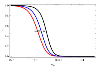
Figure 3: (Color online) The visibility $V_{+}$ vs the mean value of noise counts $N_{\mathrm{nc}}$ for different values of the turbulence parameter $\sigma$: (a) $0.1$, (b) $1$, (c) $2$. The detection efficiency is $\eta_{\mathrm{c}}=0.25$; the mean atmospheric and beam-splitter losses are $35\,\mathrm{dB}$. The result is equal for both photon-number-resolving and on/off detectors.

V Parametric down-conversion source

The realistic sources used in experiments generate radiation states, which are more complicated than the Bell state (12). For example, in Refs. Fedrizzi ; Ursin one uses a PDC source for the generation of entangled photon pairs. For such a source, the contribution from the multiphoton pair emission is essential. In the presence of losses or/and in the case of using on/off detectors, all these photons contribute to the measured Bell parameter. Moreover, the result appears to be very sensitive to the background noise and dark counts.

The state generated by the PDC source is given by (cf. PDC )

$$\left|\mathrm{PDC}\right\rangle=(\cosh\chi)^{-2}\sum\limits_{n=0}^{+\infty}\sqrt{n+1}\tanh^{n}\chi\left|\Phi_{n}\right\rangle,$$ (33)

where $\chi$ is the squeezing parameter, and

$$\left|\Phi_{n}\right\rangle=$$ (34)

$$\frac{1}{\sqrt{n+1}}\sum\limits_{m=0}^{n}e^{i\varphi m}\left|n-m\right\rangle_{\mathrm{H_{A}}}\left|m\right\rangle_{\mathrm{V_{A}}}\left|m\right\rangle_{\mathrm{H_{B}}}\left|n-m\right\rangle_{\mathrm{V_{B}}}.$$

For $n=1$, $\left|\Phi_{n}\right\rangle$ is the Bell state, cf. Eq. (12). The state (33) is Gaussian – its characteristic function of the Glauber-Sudarshan $P$ function is written as

$$\Phi_{\mathrm{in}}\left(\beta_{\mathrm{\scriptscriptstyle H_{A}}},\beta_{\mathrm{\scriptscriptstyle V_{A}}},\beta_{\mathrm{\scriptscriptstyle H_{B}}},\beta_{\mathrm{\scriptscriptstyle V_{B}}}\right) = \exp\left[-\frac{\tanh^{2}\chi\left|\beta_{\mathrm{\scriptscriptstyle V_{A}}}\right|^{2}+\tanh^{2}\chi\left|\beta_{\mathrm{\scriptscriptstyle H_{B}}}\right|^{2}-\tanh\chi\left(\beta_{\mathrm{\scriptscriptstyle V_{A}}}\beta_{\mathrm{\scriptscriptstyle H_{B}}}+\beta^{\ast}_{\mathrm{\scriptscriptstyle V_{A}}}\beta^{\ast}_{\mathrm{\scriptscriptstyle H_{B}}}\right)}{1-\tanh^{2}\chi}\right]$$

$$\times \exp\left[-\frac{\tanh^{2}\chi\left|\beta_{\mathrm{\scriptscriptstyle H_{A}}}\right|^{2}+\tanh^{2}\chi\left|\beta_{\mathrm{\scriptscriptstyle V_{B}}}\right|^{2}-\tanh\chi\left(e^{i\varphi}\beta_{\mathrm{\scriptscriptstyle H_{A}}}\beta_{\mathrm{\scriptscriptstyle V_{B}}}+e^{-i\varphi}\beta^{\ast}_{\mathrm{\scriptscriptstyle H_{A}}}\beta^{\ast}_{\mathrm{\scriptscriptstyle V_{B}}}\right)}{1-\tanh^{2}\chi}\right].$$

We apply Eq. (V) for the quantum-state input–output relations (19) and (20). In the resulting characteristic function, the variables $\left(\beta_{\mathrm{\scriptscriptstyle H_{A}}},\beta_{\mathrm{\scriptscriptstyle V_{A}}},\beta_{\mathrm{\scriptscriptstyle H_{B}}},\beta_{\mathrm{\scriptscriptstyle V_{B}}}\right)$ are transformed to the variables $\left(\beta_{\mathrm{\scriptscriptstyle T_{A}}},\beta_{\mathrm{\scriptscriptstyle R_{A}}},\beta_{\mathrm{\scriptscriptstyle T_{B}}},\beta_{\mathrm{\scriptscriptstyle R_{B}}}\right)$ using the input–output relations for the polarization analyzers (4) and (5), which should be rewritten in terms of the arguments of the characteristic function. Finally, we substitute the resulting expression in Eqs. (6) and (1), which should be also rewritten in terms of the characteristic function. The obtained result is used in Eqs. (7) and (II) for analyzing violations of Bell inequalities. For the probability $P_{\mathrm{i_{\mathrm{A}},i_{\mathrm{B}}}}\left(\theta_{\mathrm{A}},\theta_{\mathrm{B}}\right)$ we get

$$P_{\mathrm{i_{\mathrm{A}},i_{\mathrm{B}}}}\left(\theta_{\mathrm{A}},\theta_{\mathrm{B}}\right)=\left(1-\tanh^{2}\chi\right)^{4}\exp\left(-\mathbf{N}_{\mathrm{nc}}\right)$$ (36)

$$\times\left[2\left\langle\frac{C_{\mathrm{i_{\mathrm{A}}}}C_{\mathrm{i_{\mathrm{B}}}}}{C_{\mathrm{0}}^{3}}\right\rangle-\left\langle\frac{C_{\mathrm{i_{\mathrm{A}},i_{\mathrm{B}}}}}{C_{\mathrm{0}}^{2}}\right\rangle\right.$$

$$-\left.N_{i_{\mathrm{A}}}\left\langle\frac{C_{\mathrm{i_{\mathrm{B}}}}}{C_{\mathrm{0}}^{2}}\right\rangle-N_{i_{\mathrm{B}}}\left\langle\frac{C_{\mathrm{i_{\mathrm{A}}}}}{C_{\mathrm{0}}^{2}}\right\rangle+N_{i_{\mathrm{A}}}N_{i_{\mathrm{B}}}\left\langle\frac{1}{C_{\mathrm{0}}}\right\rangle\right]$$

for photon-number-resolving detectors and

$$P_{\mathrm{i_{\mathrm{A}},i_{\mathrm{B}}}}\left(\theta_{\mathrm{A}},\theta_{\mathrm{B}}\right)=\left(1-\tanh^{2}\chi\right)^{4}\exp\left(-\mathbf{N}_{\mathrm{nc}}\right)$$ (37)

$$\times\left[\left\langle\frac{e^{N_{i_{\mathrm{A}}}+N_{i_{\mathrm{B}}}}}{C_{\mathrm{0}}+C_{\mathrm{i_{\mathrm{A}}}}+C_{\mathrm{i_{\mathrm{B}}}}+C_{\mathrm{i_{\mathrm{A}},i_{\mathrm{B}}}}}\right\rangle\right.$$

$$-\left.\left\langle\frac{e^{N_{i_{\mathrm{A}}}}}{C_{\mathrm{0}}+C_{\mathrm{i_{\mathrm{A}}}}}\right\rangle-\left\langle\frac{e^{N_{i_{\mathrm{B}}}}}{C_{\mathrm{0}}+C_{\mathrm{i_{\mathrm{B}}}}}\right\rangle+\left\langle\frac{1}{C_{\mathrm{0}}}\right\rangle\right]$$

for on/off detectors. Here

$$\mathbf{N}_{\mathrm{nc}}=N_{\mathrm{T_{A}}}+N_{\mathrm{R_{A}}}+N_{\mathrm{T_{B}}}+N_{\mathrm{R_{B}}}$$ (38)

is the total number of noise counts by the four detectors. The analytical form for the coefficients $C_{\mathrm{0}}$, $C_{\mathrm{i_{\mathrm{A}}}}$, $C_{\mathrm{i_{\mathrm{B}}}}$, and $C_{\mathrm{i_{\mathrm{A}},i_{\mathrm{B}}}}$ is given in Appendix B.

Consider again the case when both receiver stations are situated in the same place (see Fedrizzi ). For simplicity we suppose all detectors to be equal and all transmission coefficients to be strongly correlated [i.e. satisfying condition (31)]. As follows from the equations in Appendix B, in this case one can combine atmospheric and detection losses in one efficiency,

$$\eta=\eta_{\mathrm{atm}}\eta_{\mathrm{c}}.$$ (39)

We suppose this efficiency to be log-normally distributed, similar to Eq. (32). In this case, the coefficients $C_{\mathrm{0}}$, $C_{\mathrm{i_{\mathrm{A}}}}$, $C_{\mathrm{i_{\mathrm{B}}}}$, and $C_{\mathrm{i_{\mathrm{A}},i_{\mathrm{B}}}}$ have the form

$$C_{\mathrm{0}}=\left\{\eta^{2}\tanh^{2}\chi-\left[1+\left(\eta-1\right)\tanh^{2}\chi\right]^{2}\right\}^{2},$$ (40)

$$C_{\mathrm{i_{\mathrm{A}}}}=C_{\mathrm{i_{\mathrm{B}}}} = \eta\left(1-\eta\right)\left(1-\tanh^{2}\chi\right)\tanh^{2}\chi$$

$$\times \left\{\eta^{2}\tanh^{2}\chi-\left[1+\left(\eta-1\right)\tanh^{2}\chi\right]^{2}\right\},$$

$$C_{\mathrm{T_{A},T_{B}}}=C_{\mathrm{R_{A},R_{B}}} = \eta^{2}\tanh^{2}\chi\left[1-\tanh^{2}\chi\right]^{2}$$

$$\times \left[\left(1-\eta\right)^{2}\tanh^{2}\chi-\sin^{2}\left(\theta_{\mathrm{A}}-\theta_{\mathrm{B}}\right)\right],$$

$$C_{\mathrm{T_{A},R_{B}}}=C_{\mathrm{R_{A},T_{B}}} = \eta^{2}\tanh^{2}\chi\left[1-\tanh^{2}\chi\right]^{2}$$

$$\times \left[\left(1-\eta\right)^{2}\tanh^{2}\chi-\cos^{2}\left(\theta_{\mathrm{A}}-\theta_{\mathrm{B}}\right)\right].$$

The realistic values of some parameters can be extracted from Ref. Fedrizzi . The value of $\bar{\theta}$ is obtained from the relation $\left\langle T^{2}\right\rangle\eta_{\mathrm{c}}\eta_{\mathrm{bs}}{=}e^{-\bar{\theta}+\frac{\sigma^{2}}{2}}$, where $\eta_{\mathrm{c}}=0.25$, $\eta_{\mathrm{bs}}=0.5$ ($3\,\mathrm{dB}$ of beam-splitter losses BS ), and $\left\langle T^{2}\right\rangle=6.3\times 10^{-4}$ ($32\,\mathrm{dB}$ of mean atmospheric losses). Hence the total single-photon losses are $41\,\mathrm{dB}$. The mean value of noise counts is $N_{\mathrm{nc}}=0.5\times 10^{-6}$ (200 counts/s from the dark counts and 200 counts/s from the background radiation in the time window of 1.25 ns).

In the case of photon-number-resolving detectors, the Bell parameter attains maximal values in the expected range (less than $2\sqrt{2}$ but larger than $2$) for small values of the squeezing parameter $\chi$ (see Fig. 4). The pronounced minimum near $\tanh\chi=0$ is caused by contributions from classical background radiation and dark counts. Similar to the case of Bell states, the fluctuating-loss channels preserve entanglement properties of light better than similar channels with standard (or slightly fluctuating) losses. This unexpected property is a consequence of contributions from random events with $\theta<\bar{\theta}$ in the postselected measurements, where $\theta=-\ln\eta$.

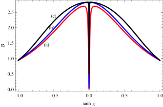
Figure 4: (Color online) The maximal value of the Bell parameter $\mathcal{B}$, obtained for photon-number-resolving detectors, vs the parameter $\tanh\chi$ for the mean value of noise counts $N_{\mathrm{nc}}=0.5\times 10^{-6}$, the mean total losses $41\,\mathrm{dB}$, and the turbulence parameter $\sigma$: (a) $0.1$, (b) $2$, (c) $3$.

The situation becomes different in the case of larger mean numbers of noise counts, e.g. $N_{\mathrm{nc}}{=}10^{-5}$. We consider this example for on/off detectors, see Fig. 5. In the case of small fluctuations (or no fluctuations) of the transmission coefficients, the maximal value of the Bell parameter may attain values less then 2 for the whole range of the parameter $\chi$. When the turbulence parameter $\sigma$ becomes rather large, contributions from events with $\theta<\bar{\theta}$ in the postselected measurements are dominant. This explains the nonclassical values of the Bell parameter for strong turbulence.

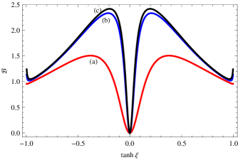
Figure 5: (Color online) The maximal value of the Bell parameter $\mathcal{B}$, obtained for on/off detectors, vs the parameter $\tanh\chi$, for the mean number of noise counts $N_{\mathrm{nc}}{=}10^{-5}$, the mean total losses $41\,\mathrm{dB}$, and the turbulence parameter $\sigma$: (a) $0.1$, (b) $2$, (c) $3$.

VI Measurement of turbulence parameters

A complete theory of quantum light in the turbulent atmosphere should include a model for the explicit form of the PDTC. Of course, the log-normal distribution (32) cannot be applied in general. Alternatively, one can consider a procedure that enables one to reconstruct the PDTC from independent measurements. Such a procedure has been proposed in Ref. Semenov1 for the case of homodyne detection of the light propagating through the atmosphere. In the considered case the situation is rather different: Since the output nonmonochromatic mode has a fluctuating form, it is difficult to measure its phase properties. On the other hand, the phase information is not necessary in the considered experiments – the corresponding equations (see for example Appendices A and B) include only mean values of the functions of $\left|T_{\mathrm{A}}\right|^{2}=\eta_{\mathrm{\scriptscriptstyle A}}$ and $\left|T_{\mathrm{B}}\right|^{2}=\eta_{\mathrm{\scriptscriptstyle B}}$. Hence, one can consider the reconstruction of the PDTC, $\mathcal{P}\left(\eta_{\mathrm{\scriptscriptstyle A}},\eta_{\mathrm{\scriptscriptstyle B}}\right)$, or alternatively, its statistical moments $\left\langle\eta_{\mathrm{\scriptscriptstyle A}}^{n}\eta_{\mathrm{\scriptscriptstyle B}}^{m}\right\rangle$.

Let the input light be prepared in coherent states, $\left|\mathrm{\alpha_{\mathrm{\scriptscriptstyle A}}}\right\rangle$ in the direction of the receiver $A$ and $\left|\mathrm{\alpha_{\mathrm{\scriptscriptstyle B}}}\right\rangle$ in the direction of the receiver $B$. For the sake of simplicity we consider a realistic situation when the resulting signal at the receivers is much stronger than the background radiation and the dark counts. In this case the photocounting distribution at the receivers is given by

$$P_{n_{\mathrm{A}},n_{\mathrm{B}}}=\int\limits_{0}^{1}\mbox{\rm d}\eta_{\mathrm{\scriptscriptstyle A}}\mbox{\rm d}\eta_{\mathrm{\scriptscriptstyle B}}\mathcal{P}\left(\eta_{\mathrm{\scriptscriptstyle A}},\eta_{\mathrm{\scriptscriptstyle B}}\right)$$ (44)

$$\times\frac{\left[\eta_{\mathrm{c}}\eta_{\mathrm{\scriptscriptstyle A}}\left|\alpha_{\mathrm{\scriptscriptstyle A}}\right|^{2}\right]^{n_{\mathrm{A}}}}{n_{\mathrm{A}}!}\frac{\left[\eta_{\mathrm{c}}\eta_{\mathrm{\scriptscriptstyle B}}\left|\alpha_{\mathrm{\scriptscriptstyle B}}\right|^{2}\right]^{n_{\mathrm{B}}}}{n_{\mathrm{B}}!}e^{-\eta_{\mathrm{c}}\left(\eta_{\mathrm{\scriptscriptstyle A}}\left|\alpha_{\mathrm{\scriptscriptstyle A}}\right|^{2}-\eta_{\mathrm{\scriptscriptstyle B}}\left|\alpha_{\mathrm{\scriptscriptstyle B}}\right|^{2}\right)},$$

where $\eta_{\mathrm{c}}$ is the detection efficiency. In principle, the methods of ill-posed problems (see, e.g., Byrne ) enable one to invert Eq. (44) and to get the PDTC, $\mathcal{P}\left(\eta_{\mathrm{\scriptscriptstyle A}},\eta_{\mathrm{\scriptscriptstyle B}}\right)$, from the measured photocounting statistics.

An alternative way to resolve this problem is the reconstruction of statistical moments of the PDTC. A mean value of a function of $\eta_{\mathrm{\scriptscriptstyle A}}$ and $\eta_{\mathrm{\scriptscriptstyle B}}$ can be presented as a series of such moments. These moments can be obtained from the corresponding moments of photocounts,

$$\overline{n_{\mathrm{A}}^{n}n_{\mathrm{B}}^{m}}=\sum\limits_{n_{\mathrm{A}},n_{\mathrm{B}}}n_{\mathrm{A}}^{n}n_{\mathrm{B}}^{m}\,P_{n_{\mathrm{A}},n_{\mathrm{B}}}.$$ (45)

For example, for the first moments, one gets

$$\overline{n_{\mathrm{A}}}=\left|\alpha_{\mathrm{\scriptscriptstyle A}}\right|^{2}\left\langle\eta_{\mathrm{\scriptscriptstyle A}}\right\rangle,$$ (46)

$$\overline{n_{\mathrm{B}}}=\left|\alpha_{\mathrm{\scriptscriptstyle B}}\right|^{2}\left\langle\eta_{\mathrm{\scriptscriptstyle B}}\right\rangle.$$ (47)

The first statistical moments of the PDTC, $\left\langle\eta_{\mathrm{\scriptscriptstyle A}}\right\rangle$ and $\left\langle\eta_{\mathrm{\scriptscriptstyle B}}\right\rangle$, are easily obtained from these equations. Similarly, the second moments of photocounts are given by

$$\overline{n_{\mathrm{A}}n_{\mathrm{B}}}=\left|\alpha_{\mathrm{\scriptscriptstyle A}}\right|^{2}\left|\alpha_{\mathrm{\scriptscriptstyle B}}\right|^{2}\left\langle\eta_{\mathrm{\scriptscriptstyle A}}\eta_{\mathrm{\scriptscriptstyle B}}\right\rangle,$$ (48)

$$\overline{n_{\mathrm{A}}^{2}}=\left|\alpha_{\mathrm{\scriptscriptstyle A}}\right|^{4}\left\langle\eta_{\mathrm{\scriptscriptstyle A}}^{2}\right\rangle+\left|\alpha_{\mathrm{\scriptscriptstyle A}}\right|^{2}\left\langle\eta_{\mathrm{\scriptscriptstyle A}}\right\rangle,$$ (49)

$$\overline{n_{\mathrm{B}}^{2}}=\left|\alpha_{\mathrm{\scriptscriptstyle B}}\right|^{4}\left\langle\eta_{\mathrm{\scriptscriptstyle B}}^{2}\right\rangle+\left|\alpha_{\mathrm{\scriptscriptstyle B}}\right|^{2}\left\langle\eta_{\mathrm{\scriptscriptstyle B}}\right\rangle.$$ (50)

Combining these equations with Eqs. (46) and (47), one gets the second statistical moments of the PDTC from $\overline{n_{\mathrm{A}}n_{\mathrm{B}}}$, $\overline{n_{\mathrm{A}}^{2}}$, $\overline{n_{\mathrm{B}}^{2}}$, $\overline{n_{\mathrm{A}}}$, and $\overline{n_{\mathrm{B}}}$. In the same way one can get higher moments of the PDTC by considering the corresponding moments of photocounts.

VII Summary and Conclusions

In recent experiments violations of Bell inequalities have been studied, by using entangled light after transmission through the turbulent atmosphere. Here we have presented analytical investigations of the transfer of entanglement through channels with fluctuating losses. The effect of the atmospheric turbulence has been modeled by the statistical properties of the complex transmission coefficient. We show how the corresponding statistical characteristics of such channels can be experimentally determined. Of course, the turbulence itself usually diminishes nonclassical properties of light. In the considered case only a small depolarization caused by the atmospheric turbulence might slightly destroy the entanglement properties of light. However, since this effect is very small it has been neglected.

For a realistic analysis of experiments, one must take into account that the measurements are usually performed in the presence of background radiation and dark counts. This may also lead, in the presence of strong losses, to a decrease of the measured value of the Bell parameter. In this context it is an important result of our treatment that fluctuating loss channels may preserve entanglement properties of light even better than the corresponding standard loss channels. The reason for this fact as follows: Some of the recorded events are related to small values of the fluctuating atmospheric transmission. These events are typically caused by background radiation and dark counts. On the other hand, for strong atmospheric turbulence the events with randomly occurring large values of the transmission coefficient will be dominant in the postselected measurements. In fact, these are the wanted events originating from the nonclassical light source.

Realistic radiation sources generate quantum states, which differ from the perfect Bell states. Important examples are parametric down-conversion sources, which are often used in experimental investigations. For such sources we study the situation for both photon-number-resolving detectors and on/off detectors. The latter appear to be very sensitive to the presence of background radiation and dark counts. We have analyzed this problem for realistic parameters. Unlike in the case of photon-number resolving detectors, for on/off detectors and for weak turbulence the Bell parameter may become extremely small. Increasing atmospheric turbulence may substantially improve this situation.

Appendix A Correlation coefficient for Bell states

Here we give the expression for the correlation coefficient $E\left(\theta_{\mathrm{A}},\theta_{\mathrm{B}}\right)$ for the Bell state (12), assuming that all detectors differ from each other. In the most general case this coefficient is given by

$$E\left(\theta_{\mathrm{A}},\theta_{\mathrm{B}}\right)$$ (51)

$$=\frac{p_{\scriptscriptstyle\mathcal{B}}E_{\scriptscriptstyle\mathcal{B}}\left(\theta_{\mathrm{A}},\theta_{\mathrm{B}}\right)+p_{\scriptscriptstyle\mathrm{H_{A}}}E_{\scriptscriptstyle\mathrm{H_{A}}}\left(\theta_{\mathrm{A}},\theta_{\mathrm{B}}\right)+p_{\scriptscriptstyle\mathrm{V_{A}}}E_{\scriptscriptstyle\mathrm{V_{A}}}\left(\theta_{\mathrm{A}},\theta_{\mathrm{B}}\right)+p_{\scriptscriptstyle\mathrm{H_{B}}}E_{\scriptscriptstyle\mathrm{H_{B}}}\left(\theta_{\mathrm{A}},\theta_{\mathrm{B}}\right)+p_{\scriptscriptstyle\mathrm{V_{B}}}E_{\scriptscriptstyle\mathrm{V_{B}}}\left(\theta_{\mathrm{A}},\theta_{\mathrm{B}}\right)+p_{\scriptscriptstyle\mathrm{0}}E_{\scriptscriptstyle\mathrm{0}}\left(\theta_{\mathrm{A}},\theta_{\mathrm{B}}\right)}{p_{\scriptscriptstyle\mathcal{B}}P_{\scriptscriptstyle\mathcal{B}}\left(\theta_{\mathrm{A}},\theta_{\mathrm{B}}\right)+p_{\scriptscriptstyle\mathrm{H_{A}}}P_{\scriptscriptstyle\mathrm{H_{A}}}\left(\theta_{\mathrm{A}},\theta_{\mathrm{B}}\right)+p_{\scriptscriptstyle\mathrm{V_{A}}}P_{\scriptscriptstyle\mathrm{V_{A}}}\left(\theta_{\mathrm{A}},\theta_{\mathrm{B}}\right)+p_{\scriptscriptstyle\mathrm{H_{B}}}P_{\scriptscriptstyle\mathrm{H_{B}}}\left(\theta_{\mathrm{A}},\theta_{\mathrm{B}}\right)+p_{\scriptscriptstyle\mathrm{V_{B}}}P_{\scriptscriptstyle\mathrm{V_{B}}}\left(\theta_{\mathrm{A}},\theta_{\mathrm{B}}\right)+p_{\scriptscriptstyle\mathrm{0}}P_{\scriptscriptstyle\mathrm{0}}\left(\theta_{\mathrm{A}},\theta_{\mathrm{B}}\right)}.$$

Here $p_{\scriptscriptstyle\mathrm{0}}$, $p_{\scriptscriptstyle\mathrm{H_{A}}}$, $p_{\scriptscriptstyle\mathrm{V_{A}}}$, $p_{\scriptscriptstyle\mathrm{H_{B}}}$, $p_{\scriptscriptstyle\mathrm{V_{B}}}$, $p_{\scriptscriptstyle\mathcal{B}}$ are given by Eqs. (23)-(26). The coefficients $E_{i}\left(\theta_{\mathrm{A}},\theta_{\mathrm{B}}\right)$ and $P_{i}\left(\theta_{\mathrm{A}},\theta_{\mathrm{B}}\right)$ ($i=\left\{0,\mathrm{H_{A}},\mathrm{V_{A}},\mathrm{H_{B}},\mathrm{V_{B}},\mathcal{B}\right\}$) have a different form for the case of photon-number resolving and on/off detectors. For photon-number resolving detectors they read as

$$E_{\scriptscriptstyle\mathrm{0}}\left(\theta_{\mathrm{A}},\theta_{\mathrm{B}}\right)=e^{-\mathbf{N}_{\mathrm{nc}}}\left(N_{\scriptscriptstyle\mathrm{T_{A}}}-N_{\scriptscriptstyle\mathrm{R_{A}}}\right)\left(N_{\scriptscriptstyle\mathrm{T_{B}}}-N_{\scriptscriptstyle\mathrm{R_{B}}}\right),$$ (52)

$$E_{\scriptscriptstyle\mathcal{B}}\left(\theta_{\mathrm{A}},\theta_{\mathrm{B}}\right){=}-\frac{1}{2}e^{-\mathbf{N}_{\mathrm{nc}}}\Big{\{}\left[\eta_{\scriptscriptstyle\mathrm{T_{A}}}{+}\left(N_{\scriptscriptstyle\mathrm{T_{A}}}{-}N_{\scriptscriptstyle\mathrm{R_{A}}}\right)\left(1{-}\eta_{\scriptscriptstyle\mathrm{T_{A}}}\right)\right]\left[\eta_{\scriptscriptstyle\mathrm{R_{B}}}{+}\left(N_{\scriptscriptstyle\mathrm{R_{B}}}{-}N_{\scriptscriptstyle\mathrm{T_{B}}}\right)\left(1{-}\eta_{\scriptscriptstyle\mathrm{R_{B}}}\right)\right]\Big{.}$$ (53)

$$\Big{.}+\left[\eta_{\scriptscriptstyle\mathrm{R_{A}}}{+}\left(N_{\scriptscriptstyle\mathrm{R_{A}}}{-}N_{\scriptscriptstyle\mathrm{T_{A}}}\right)\left(1{-}\eta_{\scriptscriptstyle\mathrm{R_{A}}}\right)\right]\left[\eta_{\scriptscriptstyle\mathrm{T_{B}}}{+}\left(N_{\scriptscriptstyle\mathrm{T_{B}}}{-}N_{\scriptscriptstyle\mathrm{R_{B}}}\right)\left(1{-}\eta_{\scriptscriptstyle\mathrm{T_{B}}}\right)\right]\Big{\}}$$

$$+\frac{1}{2}e^{-\mathbf{N}_{\mathrm{nc}}}\left[\eta_{\scriptscriptstyle\mathrm{T_{A}}}+\eta_{\scriptscriptstyle\mathrm{R_{A}}}+\left(N_{\scriptscriptstyle\mathrm{T_{A}}}{-}N_{\scriptscriptstyle\mathrm{R_{A}}}\right)\left(\eta_{\scriptscriptstyle\mathrm{R_{A}}}{-}\eta_{\scriptscriptstyle\mathrm{T_{A}}}\right)\right]\left[\eta_{\scriptscriptstyle\mathrm{T_{B}}}+\eta_{\scriptscriptstyle\mathrm{R_{B}}}+\left(N_{\scriptscriptstyle\mathrm{T_{B}}}{-}N_{\scriptscriptstyle\mathrm{R_{B}}}\right)\left(\eta_{\scriptscriptstyle\mathrm{R_{B}}}{-}\eta_{\scriptscriptstyle\mathrm{T_{B}}}\right)\right]$$

$$\times\left[\sin^{2}\left(\theta_{\mathrm{A}}{+}\theta_{\mathrm{B}}\right)\cos^{2}\frac{\varphi}{2}+\sin^{2}\left(\theta_{\mathrm{A}}{-}\theta_{\mathrm{B}}\right)\sin^{2}\frac{\varphi}{2}\right],$$

$$E_{\scriptscriptstyle\mathrm{H_{A(B)}}} \left(\theta_{\mathrm{A}},\theta_{\mathrm{B}}\right)=e^{-\mathbf{N}_{\mathrm{nc}}}\left(N_{\scriptscriptstyle\mathrm{T_{B(A)}}}-N_{\scriptscriptstyle\mathrm{R_{B(A)}}}\right)$$

$$\times\left\{\left[\eta_{\scriptscriptstyle\mathrm{T_{A(B)}}}+(1-\eta_{\scriptscriptstyle\mathrm{T_{A(B)}}})(N_{\scriptscriptstyle\mathrm{T_{A(B)}}}-N_{\scriptscriptstyle\mathrm{R_{A(B)}}})\right]\cos^{2}\theta_{\mathrm{A(B)}}-\left[\eta_{\scriptscriptstyle\mathrm{R_{A(B)}}}+(1-\eta_{\scriptscriptstyle\mathrm{R_{A(B)}}})(N_{\scriptscriptstyle\mathrm{R_{A(B)}}}-N_{\scriptscriptstyle\mathrm{T_{A(B)}}})\right]\sin^{2}\theta_{\mathrm{A(B)}}\right\},$$

$$E_{\scriptscriptstyle\mathrm{V_{A(B)}}} \left(\theta_{\mathrm{A}},\theta_{\mathrm{B}}\right)=e^{-\mathbf{N}_{\mathrm{nc}}}\left(N_{\scriptscriptstyle\mathrm{T_{B(A)}}}-N_{\scriptscriptstyle\mathrm{R_{B(A)}}}\right)$$

$$\times\left\{\left[\eta_{\scriptscriptstyle\mathrm{T_{A(B)}}}+(1-\eta_{\scriptscriptstyle\mathrm{T_{A(B)}}})(N_{\scriptscriptstyle\mathrm{T_{A(B)}}}-N_{\scriptscriptstyle\mathrm{R_{A(B)}}})\right]\sin^{2}\theta_{\mathrm{A(B)}}-\left[\eta_{\scriptscriptstyle\mathrm{R_{A(B)}}}+(1-\eta_{\scriptscriptstyle\mathrm{R_{A(B)}}})(N_{\scriptscriptstyle\mathrm{R_{A(B)}}}-N_{\scriptscriptstyle\mathrm{T_{A(B)}}})\right]\cos^{2}\theta_{\mathrm{A(B)}}\right\},$$

$$P_{\scriptscriptstyle\mathrm{0}}\left(\theta_{\mathrm{A}},\theta_{\mathrm{B}}\right)=e^{-\mathbf{N}_{\mathrm{nc}}}\left(N_{\scriptscriptstyle\mathrm{T_{A}}}+N_{\scriptscriptstyle\mathrm{R_{A}}}\right)\left(N_{\scriptscriptstyle\mathrm{T_{B}}}+N_{\scriptscriptstyle\mathrm{R_{B}}}\right),$$ (56)

$$P_{\scriptscriptstyle\mathcal{B}}\left(\theta_{\mathrm{A}},\theta_{\mathrm{B}}\right)=\frac{1}{2}e^{-\mathbf{N}_{\mathrm{nc}}}\Big{\{}\Big{.}\left[\eta_{\scriptscriptstyle\mathrm{T_{A}}}{+}\left(N_{\scriptscriptstyle\mathrm{T_{A}}}{+}N_{\scriptscriptstyle\mathrm{R_{A}}}\right)\left(1{-}\eta_{\scriptscriptstyle\mathrm{T_{A}}}\right)\right]\left[\eta_{\scriptscriptstyle\mathrm{R_{B}}}{+}\left(N_{\scriptscriptstyle\mathrm{T_{B}}}{+}N_{\scriptscriptstyle\mathrm{R_{B}}}\right)\left(1{-}\eta_{\scriptscriptstyle\mathrm{R_{B}}}\right)\right]\Big{.}$$ (57)

$$\Big{.}+\left[\eta_{\scriptscriptstyle\mathrm{R_{A}}}{+}\left(N_{\scriptscriptstyle\mathrm{T_{A}}}{+}N_{\scriptscriptstyle\mathrm{R_{A}}}\right)\left(1{-}\eta_{\scriptscriptstyle\mathrm{R_{A}}}\right)\right]\left[\eta_{\scriptscriptstyle\mathrm{T_{B}}}{+}\left(N_{\scriptscriptstyle\mathrm{T_{B}}}{+}N_{\scriptscriptstyle\mathrm{R_{B}}}\right)\left(1{-}\eta_{\scriptscriptstyle\mathrm{T_{B}}}\right)\right]\Big{.}$$

$$\Big{.}+\left[\eta_{\scriptscriptstyle\mathrm{T_{A}}}{-}\eta_{\scriptscriptstyle\mathrm{R_{A}}}\right]\left[\eta_{\scriptscriptstyle\mathrm{T_{B}}}{-}\eta_{\scriptscriptstyle\mathrm{R_{B}}}\right]\left[1{-}N_{\scriptscriptstyle\mathrm{T_{A}}}{-}N_{\scriptscriptstyle\mathrm{R_{A}}}\right]\left[1{-}N_{\scriptscriptstyle\mathrm{T_{B}}}{-}N_{\scriptscriptstyle\mathrm{R_{B}}}\right]\left[\sin^{2}\left(\theta_{\mathrm{A}}{+}\theta_{\mathrm{B}}\right)\cos^{2}\frac{\varphi}{2}+\sin^{2}\left(\theta_{\mathrm{A}}{-}\theta_{\mathrm{B}}\right)\sin^{2}\frac{\varphi}{2}\right]\Big{\}},$$

$$P_{\scriptscriptstyle\mathrm{H_{A(B)}}} \left(\theta_{\mathrm{A}},\theta_{\mathrm{B}}\right)=e^{-\mathbf{N}_{\mathrm{nc}}}\left(N_{\scriptscriptstyle\mathrm{T_{B(A)}}}+N_{\scriptscriptstyle\mathrm{R_{B(A)}}}\right)$$

$$\times\left\{\left[\eta_{\scriptscriptstyle\mathrm{T_{A(B)}}}+(1-\eta_{\scriptscriptstyle\mathrm{T_{A(B)}}})(N_{\scriptscriptstyle\mathrm{T_{A(B)}}}+N_{\scriptscriptstyle\mathrm{R_{A(B)}}})\right]\cos^{2}\theta_{\mathrm{A(B)}}+\left[\eta_{\scriptscriptstyle\mathrm{R_{A(B)}}}+(1-\eta_{\scriptscriptstyle\mathrm{R_{A(B)}}})(N_{\scriptscriptstyle\mathrm{R_{A(B)}}}+N_{\scriptscriptstyle\mathrm{T_{A(B)}}})\right]\sin^{2}\theta_{\mathrm{A(B)}}\right\},$$

$$P_{\scriptscriptstyle\mathrm{V_{A(B)}}} \left(\theta_{\mathrm{A}},\theta_{\mathrm{B}}\right)=e^{-\mathbf{N}_{\mathrm{nc}}}\left(N_{\scriptscriptstyle\mathrm{T_{B(A)}}}+N_{\scriptscriptstyle\mathrm{R_{B(A)}}}\right)$$

$$\times\left\{\left[\eta_{\scriptscriptstyle\mathrm{T_{A(B)}}}+(1-\eta_{\scriptscriptstyle\mathrm{T_{A(B)}}})(N_{\scriptscriptstyle\mathrm{T_{A(B)}}}+N_{\scriptscriptstyle\mathrm{R_{A(B)}}})\right]\sin^{2}\theta_{\mathrm{A(B)}}+\left[\eta_{\scriptscriptstyle\mathrm{R_{A(B)}}}+(1-\eta_{\scriptscriptstyle\mathrm{R_{A(B)}}})(N_{\scriptscriptstyle\mathrm{R_{A(B)}}}+N_{\scriptscriptstyle\mathrm{T_{A(B)}}})\right]\cos^{2}\theta_{\mathrm{A(B)}}\right\},$$

where $\mathbf{N}_{\mathrm{nc}}$ is the total mean value of noise counts, cf. Eq. (38). For the case of using on/off detectors the coefficients in Eq. (51) are given by

$$E_{\scriptscriptstyle\mathrm{0}}\left(\theta_{\mathrm{A}},\theta_{\mathrm{B}}\right)=e^{-\mathbf{N}_{\mathrm{nc}}}\left(e^{N_{\scriptscriptstyle\mathrm{T_{A}}}}-e^{N_{\scriptscriptstyle\mathrm{R_{A}}}}\right)\left(e^{N_{\scriptscriptstyle\mathrm{T_{B}}}}-e^{N_{\scriptscriptstyle\mathrm{R_{B}}}}\right),$$ (60)

$$E_{\scriptscriptstyle\mathcal{B}}\left(\theta_{\mathrm{A}},\theta_{\mathrm{B}}\right){=}-\frac{1}{2}e^{-\mathbf{N}_{\mathrm{nc}}}\Big{\{}\left[\eta_{\scriptscriptstyle\mathrm{T_{A}}}e^{N_{\scriptscriptstyle\mathrm{R_{A}}}}{+}e^{N_{\scriptscriptstyle\mathrm{T_{A}}}}{-}e^{N_{\scriptscriptstyle\mathrm{R_{A}}}}\right]\left[\eta_{\scriptscriptstyle\mathrm{R_{B}}}e^{N_{\scriptscriptstyle\mathrm{T_{B}}}}{+}e^{N_{\scriptscriptstyle\mathrm{R_{B}}}}{-}e^{N_{\scriptscriptstyle\mathrm{T_{B}}}}\right]\Big{.}$$ (61)

$$\Big{.}+\left[\eta_{\scriptscriptstyle\mathrm{R_{A}}}e^{N_{\scriptscriptstyle\mathrm{T_{A}}}}{+}e^{N_{\scriptscriptstyle\mathrm{R_{A}}}}{-}e^{N_{\scriptscriptstyle\mathrm{T_{A}}}}\right]\left[\eta_{\scriptscriptstyle\mathrm{T_{B}}}e^{N_{\scriptscriptstyle\mathrm{R_{B}}}}{+}e^{N_{\scriptscriptstyle\mathrm{T_{B}}}}{-}e^{N_{\scriptscriptstyle\mathrm{R_{B}}}}\right]\Big{\}}$$

$$+\frac{1}{2}e^{-\mathbf{N}_{\mathrm{nc}}}\left[\eta_{\scriptscriptstyle\mathrm{T_{A}}}e^{N_{\scriptscriptstyle\mathrm{R_{A}}}}+\eta_{\scriptscriptstyle\mathrm{R_{A}}}e^{N_{\scriptscriptstyle\mathrm{T_{A}}}}\right]\left[\eta_{\scriptscriptstyle\mathrm{T_{B}}}e^{N_{\scriptscriptstyle\mathrm{R_{B}}}}+\eta_{\scriptscriptstyle\mathrm{R_{B}}}e^{N_{\scriptscriptstyle\mathrm{T_{B}}}}\right]$$

$$\times\left[\sin^{2}\left(\theta_{\mathrm{A}}{+}\theta_{\mathrm{B}}\right)\cos^{2}\frac{\varphi}{2}+\sin^{2}\left(\theta_{\mathrm{A}}{-}\theta_{\mathrm{B}}\right)\sin^{2}\frac{\varphi}{2}\right],$$

$$E_{\scriptscriptstyle\mathrm{H_{A(B)}}}\left(\theta_{\mathrm{A}},\theta_{\mathrm{B}}\right) =e^{-\mathbf{N}_{\mathrm{nc}}}\left(e^{N_{\scriptscriptstyle\mathrm{T_{B(A)}}}}-e^{N_{\scriptscriptstyle\mathrm{R_{B(A)}}}}\right)$$

$$\times\Big{\{}\left[\eta_{\scriptscriptstyle\mathrm{T_{A(B)}}}e^{N_{\scriptscriptstyle\mathrm{T_{A(B)}}}}+(1-\eta_{\scriptscriptstyle\mathrm{T_{A(B)}}})(e^{N_{\scriptscriptstyle\mathrm{T_{A(B)}}}}-e^{N_{\scriptscriptstyle\mathrm{R_{A(B)}}}})\right]\cos^{2}\theta_{\mathrm{A(B)}}\Big{.}$$

$$\Big{.}-\left[\eta_{\scriptscriptstyle\mathrm{R_{A(B)}}}e^{N_{\scriptscriptstyle\mathrm{R_{A(B)}}}}+(1-\eta_{\scriptscriptstyle\mathrm{R_{A(B)}}})(e^{N_{\scriptscriptstyle\mathrm{R_{A(B)}}}}-e^{N_{\scriptscriptstyle\mathrm{T_{A(B)}}}})\right]\sin^{2}\theta_{\mathrm{A(B)}}\Big{\}},$$

$$E_{\scriptscriptstyle\mathrm{V_{A(B)}}}\left(\theta_{\mathrm{A}},\theta_{\mathrm{B}}\right) =e^{-\mathbf{N}_{\mathrm{nc}}}\left(e^{N_{\scriptscriptstyle\mathrm{T_{B(A)}}}}-e^{N_{\scriptscriptstyle\mathrm{R_{B(A)}}}}\right)$$

$$\times\Big{\{}\left[\eta_{\scriptscriptstyle\mathrm{T_{A(B)}}}e^{N_{\scriptscriptstyle\mathrm{T_{A(B)}}}}+(1-\eta_{\scriptscriptstyle\mathrm{T_{A(B)}}})(e^{N_{\scriptscriptstyle\mathrm{T_{A(B)}}}}-e^{N_{\scriptscriptstyle\mathrm{R_{A(B)}}}})\right]\sin^{2}\theta_{\mathrm{A(B)}}\Big{.}$$

$$\Big{.}-\left[\eta_{\scriptscriptstyle\mathrm{R_{A(B)}}}e^{N_{\scriptscriptstyle\mathrm{R_{A(B)}}}}+(1-\eta_{\scriptscriptstyle\mathrm{R_{A(B)}}})(e^{N_{\scriptscriptstyle\mathrm{R_{A(B)}}}}-e^{N_{\scriptscriptstyle\mathrm{T_{A(B)}}}})\right]\cos^{2}\theta_{\mathrm{A(B)}}\Big{\}},$$

$$P_{\scriptscriptstyle\mathrm{0}}\left(\theta_{\mathrm{A}},\theta_{\mathrm{B}}\right)=e^{-\mathbf{N}_{\mathrm{nc}}}\left(e^{N_{\scriptscriptstyle\mathrm{T_{A}}}}+e^{N_{\scriptscriptstyle\mathrm{R_{A}}}}-2\right)\left(e^{N_{\scriptscriptstyle\mathrm{T_{B}}}}+e^{N_{\scriptscriptstyle\mathrm{R_{B}}}}-2\right),$$ (64)

$$P_{\scriptscriptstyle\mathcal{B}}\left(\theta_{\mathrm{A}},\theta_{\mathrm{B}}\right)=\frac{1}{2}e^{-\mathbf{N}_{\mathrm{nc}}}\Big{\{}\Big{.}\left[\left(1{-}\eta_{\scriptscriptstyle\mathrm{T_{A}}}\right)\left(e^{N_{\scriptscriptstyle\mathrm{R_{A}}}}-2\right){+}e^{N_{\scriptscriptstyle\mathrm{T_{A}}}}\right]\left[\left(1{-}\eta_{\scriptscriptstyle\mathrm{R_{B}}}\right)\left(e^{N_{\scriptscriptstyle\mathrm{T_{B}}}}-2\right){+}e^{N_{\scriptscriptstyle\mathrm{R_{B}}}}\right]\Big{.}$$ (65)

$$\Big{.}+\left[\left(1{-}\eta_{\scriptscriptstyle\mathrm{R_{A}}}\right)\left(e^{N_{\scriptscriptstyle\mathrm{T_{A}}}}-2\right){+}e^{N_{\scriptscriptstyle\mathrm{R_{A}}}}\right]\left[\left(1{-}\eta_{\scriptscriptstyle\mathrm{T_{B}}}\right)\left(e^{N_{\scriptscriptstyle\mathrm{R_{B}}}}-2\right){+}e^{N_{\scriptscriptstyle\mathrm{T_{B}}}}\right]\Big{.}$$

$$\Big{.}+\left[2\left(\eta_{\scriptscriptstyle\mathrm{T_{A}}}{-}\eta_{\scriptscriptstyle\mathrm{R_{A}}}\right){+}\eta_{\scriptscriptstyle\mathrm{R_{A}}}e^{N_{\scriptscriptstyle\mathrm{T_{A}}}}{-}\eta_{\scriptscriptstyle\mathrm{T_{A}}}e^{N_{\scriptscriptstyle\mathrm{R_{A}}}}\right]\left[2\left(\eta_{\scriptscriptstyle\mathrm{T_{B}}}{-}\eta_{\scriptscriptstyle\mathrm{R_{B}}}\right){+}\eta_{\scriptscriptstyle\mathrm{R_{B}}}e^{N_{\scriptscriptstyle\mathrm{T_{B}}}}{-}\eta_{\scriptscriptstyle\mathrm{T_{B}}}e^{N_{\scriptscriptstyle\mathrm{R_{B}}}}\right]$$

$$\times\left[\sin^{2}\left(\theta_{\mathrm{A}}{+}\theta_{\mathrm{B}}\right)\cos^{2}\frac{\varphi}{2}+\sin^{2}\left(\theta_{\mathrm{A}}{-}\theta_{\mathrm{B}}\right)\sin^{2}\frac{\varphi}{2}\right]\Big{\}},$$

$$P_{\scriptscriptstyle\mathrm{H_{A(B)}}}\left(\theta_{\mathrm{A}},\theta_{\mathrm{B}}\right) =e^{-\mathbf{N}_{\mathrm{nc}}}\left(e^{N_{\scriptscriptstyle\mathrm{T_{B(A)}}}}+e^{N_{\scriptscriptstyle\mathrm{R_{B(A)}}}}-2\right)$$

$$\times\Big{\{}\left[\eta_{\scriptscriptstyle\mathrm{T_{A(B)}}}e^{N_{\scriptscriptstyle\mathrm{T_{A(B)}}}}+(1-\eta_{\scriptscriptstyle\mathrm{T_{A(B)}}})(e^{N_{\scriptscriptstyle\mathrm{T_{A(B)}}}}+e^{N_{\scriptscriptstyle\mathrm{R_{A(B)}}}}-2)\right]\cos^{2}\theta_{\mathrm{A(B)}}\Big{.}$$

$$\Big{.}-\left[\eta_{\scriptscriptstyle\mathrm{R_{A(B)}}}e^{N_{\scriptscriptstyle\mathrm{R_{A(B)}}}}+(1-\eta_{\scriptscriptstyle\mathrm{R_{A(B)}}})(e^{N_{\scriptscriptstyle\mathrm{R_{A(B)}}}}+e^{N_{\scriptscriptstyle\mathrm{T_{A(B)}}}}-2)\right]\sin^{2}\theta_{\mathrm{A(B)}}\Big{\}},$$

$$P_{\scriptscriptstyle\mathrm{V_{A(B)}}}\left(\theta_{\mathrm{A}},\theta_{\mathrm{B}}\right) =e^{-\mathbf{N}_{\mathrm{nc}}}\left(e^{N_{\scriptscriptstyle\mathrm{T_{B(A)}}}}+e^{N_{\scriptscriptstyle\mathrm{R_{B(A)}}}}-2\right)$$

$$\times\Big{\{}\left[\eta_{\scriptscriptstyle\mathrm{T_{A(B)}}}e^{N_{\scriptscriptstyle\mathrm{T_{A(B)}}}}+(1-\eta_{\scriptscriptstyle\mathrm{T_{A(B)}}})(e^{N_{\scriptscriptstyle\mathrm{T_{A(B)}}}}+e^{N_{\scriptscriptstyle\mathrm{R_{A(B)}}}}-2)\right]\sin^{2}\theta_{\mathrm{A(B)}}\Big{.}$$

$$\Big{.}+\left[\eta_{\scriptscriptstyle\mathrm{R_{A(B)}}}e^{N_{\scriptscriptstyle\mathrm{R_{A(B)}}}}+(1-\eta_{\scriptscriptstyle\mathrm{R_{A(B)}}})(e^{N_{\scriptscriptstyle\mathrm{R_{A(B)}}}}-e^{N_{\scriptscriptstyle\mathrm{T_{A(B)}}}}-2)\right]\cos^{2}\theta_{\mathrm{A(B)}}\Big{\}}.$$

Appendix B Coefficients in the detection probabilities for the parametric down-conversion source

Here we give the explicit form of the coefficients $C_{\mathrm{0}}$, $C_{\mathrm{i_{\mathrm{A}}}}$, $C_{\mathrm{i_{\mathrm{B}}}}$, and $C_{\mathrm{i_{\mathrm{A}},i_{\mathrm{B}}}}$ in the most general case. These coefficients appear in the expressions for the probabilities $P_{\mathrm{i_{\mathrm{A}},i_{\mathrm{B}}}}\left(\theta_{\mathrm{A}},\theta_{\mathrm{B}}\right)$, cf. Eqs. (36) and (37), in the case of using a PDC source of entangled photons. They are given by

$$C_{\mathrm{0}}=\left[1+\left(\Omega_{\mathrm{T_{A}}}-1\right)\tanh^{2}\chi\right]\left[1+\left(\Omega_{\mathrm{R_{A}}}-1\right)\tanh^{2}\chi\right]\left[1+\left(\Omega_{\mathrm{T_{B}}}-1\right)\tanh^{2}\chi\right]\left[1+\left(\Omega_{\mathrm{R_{B}}}-1\right)\tanh^{2}\chi\right]$$ (68)

$$-\left[1+\left(\Omega_{\mathrm{T_{A}}}-1\right)\tanh^{2}\chi\right]\left[1+\left(\Omega_{\mathrm{T_{B}}}-1\right)\tanh^{2}\chi\right]D_{\mathrm{T_{A},T_{B}}}-\left[1+\left(\Omega_{\mathrm{T_{A}}}-1\right)\tanh^{2}\chi\right]\left[1+\left(\Omega_{\mathrm{R_{B}}}-1\right)\tanh^{2}\chi\right]D_{\mathrm{T_{A},R_{B}}}$$

$$-\left[1+\left(\Omega_{\mathrm{R_{A}}}-1\right)\tanh^{2}\chi\right]\left[1+\left(\Omega_{\mathrm{R_{B}}}-1\right)\tanh^{2}\chi\right]D_{\mathrm{R_{A},R_{B}}}-\left[1+\left(\Omega_{\mathrm{R_{A}}}-1\right)\tanh^{2}\chi\right]\left[1+\left(\Omega_{\mathrm{T_{B}}}-1\right)\tanh^{2}\chi\right]D_{\mathrm{R_{A},T_{B}}}$$

$$+D_{\mathrm{0}},$$

$$C_{\mathrm{T_{A}}}=-\Omega_{\mathrm{T_{A}}}\left[1+\left(\Omega_{\mathrm{R_{A}}}-1\right)\tanh^{2}\chi\right]\left[1+\left(\Omega_{\mathrm{T_{B}}}-1\right)\tanh^{2}\chi\right]\left[1+\left(\Omega_{\mathrm{R_{B}}}-1\right)\tanh^{2}\chi\right]$$ (69)

$$+\Omega_{\mathrm{T_{A}}}\tanh^{2}\chi\left[1+\left(\Omega_{\mathrm{T_{B}}}-1\right)\tanh^{2}\chi\right]D_{\mathrm{T_{A},T_{B}}}+\Omega_{\mathrm{T_{A}}}\tanh^{2}\chi\left[1+\left(\Omega_{\mathrm{R_{B}}}-1\right)\tanh^{2}\chi\right]D_{\mathrm{T_{A},R_{B}}}$$

$$+\left[1+\left(\Omega_{\mathrm{R_{A}}}-1\right)\tanh^{2}\chi\right]\left[1+\left(\Omega_{\mathrm{R_{B}}}-1\right)\tanh^{2}\chi\right]D_{\mathrm{R_{A},R_{B}}}+\left[1+\left(\Omega_{\mathrm{R_{A}}}-1\right)\tanh^{2}\chi\right]\left[1+\left(\Omega_{\mathrm{T_{B}}}-1\right)\tanh^{2}\chi\right]D_{\mathrm{R_{A},T_{B}}}$$

$$-D_{\mathrm{0}},$$

$$C_{\mathrm{R_{A}}}=-\Omega_{\mathrm{R_{A}}}\tanh^{2}\chi\left[1+\left(\Omega_{\mathrm{T_{A}}}-1\right)\tanh^{2}\chi\right]\left[1+\left(\Omega_{\mathrm{T_{B}}}-1\right)\tanh^{2}\chi\right]\left[1+\left(\Omega_{\mathrm{R_{B}}}-1\right)\tanh^{2}\chi\right]$$ (70)

$$+\left[1+\left(\Omega_{\mathrm{T_{A}}}-1\right)\tanh^{2}\chi\right]\left[1+\left(\Omega_{\mathrm{T_{B}}}-1\right)\tanh^{2}\chi\right]D_{\mathrm{T_{A},T_{B}}}+\left[1+\left(\Omega_{\mathrm{T_{A}}}-1\right)\tanh^{2}\chi\right]\left[1+\left(\Omega_{\mathrm{R_{B}}}-1\right)\tanh^{2}\chi\right]D_{\mathrm{T_{A},R_{B}}}$$

$$+\Omega_{\mathrm{R_{A}}}\tanh^{2}\chi\left[1+\left(\Omega_{\mathrm{R_{B}}}-1\right)\tanh^{2}\chi\right]D_{\mathrm{R_{A},R_{B}}}+\Omega_{\mathrm{R_{A}}}\tanh^{2}\chi\left[1+\left(\Omega_{\mathrm{T_{B}}}-1\right)\tanh^{2}\chi\right]D_{\mathrm{R_{A},T_{B}}}$$

$$-D_{\mathrm{0}},$$

$$C_{\mathrm{T_{B}}}=-\Omega_{\mathrm{T_{B}}}\tanh^{2}\chi\left[1+\left(\Omega_{\mathrm{T_{A}}}-1\right)\tanh^{2}\chi\right]\left[1+\left(\Omega_{\mathrm{R_{A}}}-1\right)\tanh^{2}\chi\right]\left[1+\left(\Omega_{\mathrm{R_{B}}}-1\right)\tanh^{2}\chi\right]$$ (71)

$$+\Omega_{\mathrm{T_{B}}}\tanh^{2}\chi\left[1+\left(\Omega_{\mathrm{T_{A}}}-1\right)\tanh^{2}\chi\right]D_{\mathrm{T_{A},T_{B}}}+\left[1+\left(\Omega_{\mathrm{T_{A}}}-1\right)\tanh^{2}\chi\right]\left[1+\left(\Omega_{\mathrm{R_{B}}}-1\right)\tanh^{2}\chi\right]D_{\mathrm{T_{A},R_{B}}}$$

$$+\left[1+\left(\Omega_{\mathrm{R_{A}}}-1\right)\tanh^{2}\chi\right]\left[1+\left(\Omega_{\mathrm{R_{B}}}-1\right)\tanh^{2}\chi\right]D_{\mathrm{R_{A},R_{B}}}+\Omega_{\mathrm{T_{B}}}\tanh^{2}\chi\left[1+\left(\Omega_{\mathrm{R_{A}}}-1\right)\tanh^{2}\chi\right]D_{\mathrm{R_{A},T_{B}}}$$

$$-D_{\mathrm{0}},$$

$$C_{\mathrm{R_{B}}}=-\Omega_{\mathrm{R_{B}}}\tanh^{2}\chi\left[1+\left(\Omega_{\mathrm{T_{A}}}-1\right)\tanh^{2}\chi\right]\left[1+\left(\Omega_{\mathrm{R_{A}}}-1\right)\tanh^{2}\chi\right]\left[1+\left(\Omega_{\mathrm{T_{B}}}-1\right)\tanh^{2}\chi\right]$$ (72)

$$+\left[1+\left(\Omega_{\mathrm{T_{A}}}-1\right)\tanh^{2}\chi\right]\left[1+\left(\Omega_{\mathrm{T_{B}}}-1\right)\tanh^{2}\chi\right]D_{\mathrm{T_{A},T_{B}}}+\Omega_{\mathrm{R_{B}}}\tanh^{2}\chi\left[1+\left(\Omega_{\mathrm{T_{A}}}-1\right)\tanh^{2}\chi\right]D_{\mathrm{T_{A},R_{B}}}$$

$$+\Omega_{\mathrm{R_{B}}}\tanh^{2}\chi\left[1+\left(\Omega_{\mathrm{R_{A}}}-1\right)\tanh^{2}\chi\right]D_{\mathrm{R_{A},R_{B}}}+\left[1+\left(\Omega_{\mathrm{R_{A}}}-1\right)\tanh^{2}\chi\right]\left[1+\left(\Omega_{\mathrm{T_{B}}}-1\right)\tanh^{2}\chi\right]D_{\mathrm{R_{A},T_{B}}}$$

$$-D_{\mathrm{0}},$$

$$C_{\mathrm{T_{A},T_{B}}}=\Omega_{\mathrm{T_{A}}}\Omega_{\mathrm{T_{B}}}\tanh^{4}\chi\left[1+\left(\Omega_{\mathrm{R_{A}}}-1\right)\tanh^{2}\chi\right]\left[1+\left(\Omega_{\mathrm{R_{B}}}-1\right)\tanh^{2}\chi\right]$$ (73)

$$-\Omega_{\mathrm{T_{A}}}\Omega_{\mathrm{T_{B}}}\tanh^{4}\chi D_{\mathrm{T_{A},T_{B}}}-\Omega_{\mathrm{T_{A}}}\tanh^{2}\chi\left[1+\left(\Omega_{\mathrm{R_{B}}}-1\right)\tanh^{2}\chi\right]D_{\mathrm{T_{A},R_{B}}}$$

$$-\left[1+\left(\Omega_{\mathrm{R_{A}}}-1\right)\tanh^{2}\chi\right]\left[1+\left(\Omega_{\mathrm{R_{B}}}-1\right)\tanh^{2}\chi\right]D_{\mathrm{R_{A},R_{B}}}-\Omega_{\mathrm{T_{B}}}\tanh^{2}\chi\left[1+\left(\Omega_{\mathrm{R_{A}}}-1\right)\tanh^{2}\chi\right]D_{\mathrm{R_{A},T_{B}}}$$

$$+D_{\mathrm{0}},$$

$$C_{\mathrm{T_{A},R_{B}}}=\Omega_{\mathrm{T_{A}}}\Omega_{\mathrm{R_{B}}}\tanh^{4}\chi\left[1+\left(\Omega_{\mathrm{R_{A}}}-1\right)\tanh^{2}\chi\right]\left[1+\left(\Omega_{\mathrm{T_{B}}}-1\right)\tanh^{2}\chi\right]$$ (74)

$$-\Omega_{\mathrm{T_{A}}}\tanh^{2}\chi\left[1+\left(\Omega_{\mathrm{T_{B}}}-1\right)\tanh^{2}\chi\right]D_{\mathrm{T_{A},T_{B}}}-\Omega_{\mathrm{T_{A}}}\Omega_{\mathrm{R_{B}}}\tanh^{4}\chi D_{\mathrm{T_{A},R_{B}}}$$

$$-\Omega_{\mathrm{R_{B}}}\tanh^{2}\chi\left[1+\left(\Omega_{\mathrm{R_{A}}}-1\right)\tanh^{2}\chi\right]D_{\mathrm{R_{A},R_{B}}}-\left[1+\left(\Omega_{\mathrm{R_{A}}}-1\right)\tanh^{2}\chi\right]\left[1+\left(\Omega_{\mathrm{T_{B}}}-1\right)\tanh^{2}\chi\right]D_{\mathrm{R_{A},T_{B}}}$$

$$+D_{\mathrm{0}},$$

$$C_{\mathrm{R_{A},T_{B}}}=\Omega_{\mathrm{R_{A}}}\Omega_{\mathrm{T_{B}}}\tanh^{4}\chi\left[1+\left(\Omega_{\mathrm{T_{A}}}-1\right)\tanh^{2}\chi\right]\left[1+\left(\Omega_{\mathrm{R_{B}}}-1\right)\tanh^{2}\chi\right]$$ (75)

$$-\Omega_{\mathrm{T_{B}}}\tanh^{2}\chi\left[1+\left(\Omega_{\mathrm{T_{A}}}-1\right)\tanh^{2}\chi\right]D_{\mathrm{T_{A},T_{B}}}-\left[1+\left(\Omega_{\mathrm{T_{A}}}-1\right)\tanh^{2}\chi\right]\left[1+\left(\Omega_{\mathrm{R_{B}}}-1\right)\tanh^{2}\chi\right]D_{\mathrm{T_{A},R_{B}}}$$

$$-\Omega_{\mathrm{R_{A}}}\tanh^{2}\chi\left[1+\left(\Omega_{\mathrm{R_{B}}}-1\right)\tanh^{2}\chi\right]D_{\mathrm{R_{A},R_{B}}}-\Omega_{\mathrm{R_{A}}}\Omega_{\mathrm{T_{B}}}\tanh^{4}\chi D_{\mathrm{R_{A},T_{B}}}$$

$$+D_{\mathrm{0}},$$

$$C_{\mathrm{R_{A},R_{B}}}=\Omega_{\mathrm{R_{A}}}\Omega_{\mathrm{R_{B}}}\tanh^{4}\chi\left[1+\left(\Omega_{\mathrm{T_{A}}}-1\right)\tanh^{2}\chi\right]\left[1+\left(\Omega_{\mathrm{T_{B}}}-1\right)\tanh^{2}\chi\right]$$ (76)

$$-\left[1+\left(\Omega_{\mathrm{T_{A}}}-1\right)\tanh^{2}\chi\right]\left[1+\left(\Omega_{\mathrm{T_{B}}}-1\right)\tanh^{2}\chi\right]D_{\mathrm{T_{A},T_{B}}}-\Omega_{\mathrm{R_{B}}}\tanh^{2}\chi\left[1+\left(\Omega_{\mathrm{T_{A}}}-1\right)\tanh^{2}\chi\right]D_{\mathrm{T_{A},R_{B}}}$$

$$-\Omega_{\mathrm{R_{A}}}\Omega_{\mathrm{R_{B}}}\tanh^{4}\chi D_{\mathrm{R_{A},R_{B}}}-\Omega_{\mathrm{R_{A}}}\tanh^{2}\chi\left[1+\left(\Omega_{\mathrm{T_{B}}}-1\right)\tanh^{2}\chi\right]D_{\mathrm{R_{A},T_{B}}}$$

$$+D_{\mathrm{0}},$$

where

$$D_{\mathrm{T_{A},T_{B}}}=\Omega_{\mathrm{R_{A}}}\Omega_{\mathrm{R_{B}}}\tanh^{2}\chi\left|e^{-i\varphi}\sin\theta_{\mathrm{A}}\cos\theta_{\mathrm{B}}+\cos\theta_{\mathrm{A}}\sin\theta_{\mathrm{B}}\right|^{2},$$ (77)

$$D_{\mathrm{T_{A},R_{B}}}=\Omega_{\mathrm{R_{A}}}\Omega_{\mathrm{T_{B}}}\tanh^{2}\chi\left|e^{-i\varphi}\sin\theta_{\mathrm{A}}\sin\theta_{\mathrm{B}}-\cos\theta_{\mathrm{A}}\cos\theta_{\mathrm{B}}\right|^{2},$$ (78)

$$D_{\mathrm{R_{A},R_{B}}}=\Omega_{\mathrm{T_{A}}}\Omega_{\mathrm{T_{B}}}\tanh^{2}\chi\left|-e^{-i\varphi}\cos\theta_{\mathrm{A}}\sin\theta_{\mathrm{B}}-\sin\theta_{\mathrm{A}}\cos\theta_{\mathrm{B}}\right|^{2},$$ (79)

$$D_{\mathrm{R_{A},T_{B}}}=\Omega_{\mathrm{T_{A}}}\Omega_{\mathrm{R_{B}}}\tanh^{2}\chi\left|-e^{-i\varphi}\cos\theta_{\mathrm{A}}\cos\theta_{\mathrm{B}}+\sin\theta_{\mathrm{A}}\sin\theta_{\mathrm{B}}\right|^{2},$$ (80)

$$D_{\mathrm{0}}=\Omega_{\mathrm{T_{A}}}\Omega_{\mathrm{R_{A}}}\Omega_{\mathrm{T_{B}}}\Omega_{\mathrm{R_{B}}}\tanh^{4}\chi,$$ (81)

$$\Omega_{\mathrm{T_{A(B)}}}=\eta_{\scriptscriptstyle\mathrm{T_{A(B)}}}\left|T_{\mathrm{A(B)}}\right|^{2},$$ (82)

$$\Omega_{\mathrm{R_{A(B)}}}=\eta_{\scriptscriptstyle\mathrm{R_{A(B)}}}\left|T_{\mathrm{A(B)}}\right|^{2}.$$ (83)