A cosmological viewpoint on the correspondence between deformed phase-space and canonical quantization

Abstract

We employ the familiar canonical quantization procedure in a given cosmological setting to argue that it is equivalent to and results in the same physical picture if one considers the deformation of the phase-space instead. To show this we use a Probabilistic Evolutionary Process (PEP) to make the solutions of these different approaches comparable. Specific model theories are used to show that the independent solutions of the resulting Wheeler-DeWitt equation are equivalent to solutions of the deformation method with different signs for the deformation parameter. We also argued that since the Wheeler-DeWitt equation is a direct consequence of diffeomorphism invariance, this equivalence is only true provided that the deformation of phase-space does not break such an invariance.
PACS: 98.80.Qc

1 Introduction

Standard cosmological models based on classical general relativity have no convincing and precise answer for the presence of the so-called “Big-Bang” singularity. Any hope of dealing with such singularities would be in vein unless a reliable quantum theory of gravity can be constructed. In the absence of a full theory of quantum gravity, it would be useful to describe the quantum states of the universe within the context of quantum cosmology, introduced in the works of DeWitt [1] and later Misner [2]. In this formalism which is based on the canonical quantization procedure, one first freezes a large number of degrees of freedom and then quantizes the remaining ones. The quantum state of the universe so obtained is then described by a wave function in the mini-superspace, a function of the 3-geometry of the model and matter fields presented in the theory, satisfying the Wheeler-DeWitt (WD) equation. In more recent times, the research in this area has been quite active with different approaches [3], see [4] for a review. Interesting applications can be found in [5] where canonical quantization is applied to many models with different matter fields as the source of gravity.

An important ingredient in any model theory related to the quantization of a cosmological model is the choice of the quantization procedure used to quantized the system. As mentioned above, the most widely used method has traditionally been the canonical quantization method based on the WD equation which is nothing but the application of the Hamiltonian constraint to the wave function of the universe. However, one may solve the constraint before using it in the theory and in particular, before quantizing the system. If we do so, we are led to a Schrödinger type equation where a time reparameterization in terms of various dynamical variables can be done before quantization [6, 7, 8]. A particularly interesting but rarely used approach to study quantum effects is to introduce a deformation in the phase-space of the system. It is believed that such a deformation of phase-space is an equivalent path to quantization, in particular to canonical and path integral quantizations [9].

An important question then naturally arises in applying the various quantization methods to cosmological models, that is, if they are equivalent. To at least partially answer the above question, we propose to quantize some simple cosmological models, namely the de Sitter, dusty FRW, FRW with radiative matter and Bianchi type I, using the methods described above. First we introduce a deformation to the Poisson algebra of the corresponding phase-space of the models. This will lead us to a deformed Hamiltonian from which the equations of motion can be constructed. We will show that the presence of the deformation parameter in the solutions can be interpreted as a quantum effect. This is done by comparing the resulting solutions with that of the other quantization method which is nothing but the usual canonical WD approach. Indeed, we will show that both of these quantization methods have the same physical interpretation for our chosen models.

A remark on the WD approach is that, as is well known, in canonical quantization the evolution of states disappear since in all diffeomorphism invariant theories the Hamiltonian becomes a constraint. Indeed, the wave function in the WD equation is independent of time, i.e. the universe has a static picture in this scenario. On the other hand in the deformed phase-space method, time does appear and so the evolution becomes meaningful. Therefore, the problem of the evolution of states which is a major problem in quantum cosmology may also be addressed in this approach. To propose a possible solution to this problem we will use what we call the “Probabilistic Evolutionary Process” which was introduced in [10, 11]. This mechanism is briefly studied in the next section because of its crucial role in this work. In section 3 we review the quantization of the de Sitter and dusty FRW cosmological models inspired by the Deformed Special Relativity (DSR), discussed in [12, 13]. The canonical quantization for both models will be studied in section 4. We will close the paper with a discussion and comparison of the results.

2 Probabilistic Evolutionary Process (PEP)

To quantize a classical model the following procedure is usually followed. The classical Hamiltonian is written in its corresponding operator form and the resulting Schrödinger equation obtained after quantization, i.e. $i\hbar\frac{\partial}{\partial t}\Psi={\cal{H}}\Psi$, becomes the relevant equation to describe time evolution of the quantum states. However, in diffeomorphism invariant models the Hamiltonian becomes a constraint, ${\cal{H}}=0$, and therefore does not provide for the evolution of the correspond states. This means that in such models all the states are stationary. One of the common examples of this situation is general relativity which is employed to investigate the evolution of the cosmos. In quantum cosmology, the Schrödinger equation becomes the Wheeler-DeWitt equation, ${\cal{H}}\Psi=0$. As is well known, quantum cosmology suffers from a number of problems, namely the construction of the Hilbert space for defining a positive definite inner product of the solutions of the WD equation, the operator ordering problem and most importantly, the problem of time; the wave function in the WD equation is independent of time, i.e. the universe has a static picture in this scenario. This problem was first addressed in [1] by DeWitt himself. However, he argued that the problem of time should not be considered as a hinderance in the sense that the theory itself must include a suitable well-defined time in terms of its geometry or matter fields. In this scheme time is identified with one of the characters of the geometry, usually the scale factor and is referred to as the intrinsic time, or with the momentum conjugate to the scale factor or even with a scalar character of the matter fields coupled to gravity in any specific model, known as the extrinsic time.

In general, the crucial problem in canonical quantum gravity is the presence of constraints in the gravitational field equations. Identification of time with one of the dynamical variables depends on the method we use to deal with theses constraints. Different approaches arising from these methods have been investigated in details in [6]. As discussed in [6], time may be identified before or after quantization has been done. There are approaches, on the other hand, in which time has no fundamental role. The problem is how one can describe the evolution of the universe since observations show that the universe is not presently in a stationary state. In a previous work [10, 11], we introduced a mechanism which we have called the Probabilistic Evolutionary Process (PEP), based on the probabilistic structure of quantum systems, to provide a sense of the evolution embedded in the wave function of the universe. This is based on the fact that in quantum systems the square of a state defines the probability, ${\cal{P}}_{a}=|\Psi(a)|^{2}$. The mechanism introduced as PEP says that the state $\Psi_{a}$ makes a transition to the state $\Psi_{a+da}$ if their distance, $da$, is infinitesimal and continuous, and that the higher the value of the transition probability the larger the value of ${\cal{P}}_{a+da}-{\cal{P}}_{a}$. The mechanism for transition from one state to another is through a small external perturbation. To make the discussion above more clear, we take an example which we shall encounter later on but will present the result in the form of the following figure. In what follows, we shall focus on the probabilistic description of our quantum states provided by figure 1 without worrying about the details of the model of which the figure is a result.

Figure 1: Figure used to explain the idea of PEP.

Let us take a specific initial condition, say $a=2.5$, corresponding to the point $P$. Then, PEP states that the system (here specified by the scale factor $a$) moves continuously to a state with higher probability and thus $P$ moves to the right to reach the point $Q$, a local maximum. Here, since $Q$ locally has the maximum probability the system stays at $Q$. This means that the scale factor becomes constant as the time passes. We show this transition by $P{\buildrel{PEP}\over{\longrightarrow}}Q$. Now let the initial condition be the point $R$. Then we have $R{\buildrel{PEP}\over{\longrightarrow}}Q$, and so on. Note that $R{\buildrel{PEP}\over{\longrightarrow}}S$ is possible but it has much smaller probability compared to the transitions $R{\buildrel{PEP}\over{\longrightarrow}}Q$. We note that the transitions $R{\buildrel{PEP}\over{\longrightarrow}}S$ and $S{\buildrel{PEP}\over{\longrightarrow}}T$ may be interpreted as tunnelling precesses in ordinary quantum mechanics in the sense that the probability of being at $S$ is zero. It means that PEP can reproduce tunnelling processes but with a very small probability.

In the following we will use PEP to describe the evolution of quantum cosmological states in the canonical method of quantization. We insist that PEP plays a crucial role in the interpretation of the states in canonical quantization and allows them to be compared to the states resulting from quantization by deformation of the phase-space structure.

3 Phase-space deformation: a procedure for quantization

It has long been argued that a deformation in phase-space can be seen as an alternative path to quantization, based on Wigner quasi-distribution function and Weyl correspondence between quantum-mechanical operators in Hilbert space and ordinary c-number functions in phase-space, see for example [9] and the references therein. The deformation in the usual phase-space structure is introduced by Moyal brackets which are based on the Moyal product [15]. However, to introduce such deformations it is more convenient to work with Poisson brackets rather than Moyal brackets.

From a cosmological point of view, models are built in a minisuper-(phase)-space. It is therefore safe to say that studying such a space in the presence of deformations mentioned above can be interpreted as studying the quantum effects on cosmological solutions. One should note that in gravity the effects of quantization are woven into the existence of a fundamental length [16]. The question then arises as to what form of deformations in phase-space is appropriate for studying quantum effects in a cosmological model? Studies in noncommutative geometry [17] and generalized uncertainty principle (GUP) [18] have been a source of inspiration for those who have been seeking an answer to the above question. More precisely, introduction of modifications in the structure of geometry in the way of noncommutativity has become the basis from which similar modifications in the phase-space have been inspired. In this approach, the fields and their conjugate momenta play the role of coordinate basis in noncommutative geometry [19]. In doing so an effective model is constructed whose validity will depend on its power of prediction. For example, if in a model field theory the fields are taken as noncommutative, as has been done in [19], the resulting effective theory predicts the same Lorentz violation as a field theory in which the coordinates are considered as noncommutative [20]. As a further example, it is well known that string theory can be used to suggest a modification in the bracket structure of coordinates, also known as GUP [18] which is used to modify the phase-space structure [21]. Over the years, a large number of works on noncommutative fields [15] have been inspired by noncommutative geometry model theories [17].

In this paper we study the effects of the existence of a fundamental length in a cosmological scenario by constructing a model based on the noncommutative structure of the Deformed (Doubly) Special Relativity [22] which is related to what is known as the $\kappa$-deformation [23]. This way of introducing noncommutativity is interesting because of its compatibility with Lorentz symmetry, as is commonly believed [23, 24]. The $\kappa$-deformation is introduced and studied in [25]. The $\kappa$-Minkowski space [26] arises naturally from the $\kappa$-Poincare algebra [22] such that the ordinary Poisson brackets between the coordinates are replaced by

$$\left\{x_{0},x_{i}\right\}=\frac{1}{\kappa}x_{i},$$ (1)

where $\kappa$ is the deformation (noncommutative) parameter which has the dimension of mass $\kappa=\epsilon\ell^{-1}$ when $c=\hbar=1$, and $\epsilon=\pm 1$ [27] such that $\kappa$ and $\ell$ are interpreted as dimensional parameters which are identified with the fundamental energy and length, respectively. As mentioned above, one can change the structure of the phase-space based on equation (1). Here we will examine a new kind of modification in the phase-space structure inspired by relation (1), much the same as has been done in [15, 21, 28]. In what follows we introduce noncommutativity based on $\kappa$-Minkowskian space and study its consequences on the de Sitter and dusty FRW cosmologies.

Let us start by briefly studying the ordinary, spatially flat FRW model where the metric is given by

$$ds^{2}=-N^{2}(t)dt^{2}+a^{2}(t)(dx^{2}+dy^{2}+dz^{2}),$$ (2)

with $N(t)$ being the lapse function. The Einstein-Hilbert Lagrangian with a general energy density $V(a)$ becomes

$${\cal{L}} = \sqrt{-g}(R[g]-V(a))$$ (3)

$$= -6N^{-1}a\dot{a}^{2}-Na^{3}V(a),$$

where $R[g]$ is the Ricci scalar and in the second line the total derivative term has been ignored. The corresponding Hamiltonian up to a sign becomes

$${\cal{H}}_{0} = \frac{1}{24}Na^{-1}p_{a}^{2}-Na^{3}V(a).$$ (4)

Here, we note that since the momentum conjugate to $N(t)$, $\pi=\frac{\partial{\cal{L}}}{\partial\dot{N}}$ vanishes, the term $\lambda\pi$ must be added as a constraint to Hamiltonian (4). The Dirac Hamiltonian then becomes

$${\cal{H}} = \frac{1}{24}Na^{-1}p_{a}^{2}-Na^{3}V(a)+\lambda\pi.$$ (5)

To introduce noncommutativity one can start with

$$\{N^{\prime}(t),a^{\prime}(t)\}=\ell a^{\prime}(t).$$ (6)

This is similar to equation (1) since one can interpret $N(t)$ and $a(t)$, appearing as the coefficients of $dt$ and $d\vec{x}$, in the same manner as $x_{0}$ and $x_{i}$ appearing in (1) respectively. For this reason we shall call it the $\kappa$-Minkowskian-minisuper-phase-space. In this case the Hamiltonian becomes

$${\cal{H}}^{\prime}_{0} = \frac{1}{24}N^{\prime}a^{\prime-1}{p^{\prime}}_{a}^{2}-N^{\prime}{a^{\prime}}^{3}V(a^{\prime}),$$ (7)

where the ordinary Poisson brackets are satisfied except in (6). To move along, one introduces the following variables [12, 13, 29]

$$\left\{\begin{array}[]{ll}N^{\prime}(t)=N(t)-\ell a(t)p_{a}(t),\\ a^{\prime}(t)=a(t),\\ p^{\prime}_{a}(t)=p_{a}(t).\end{array}\right.$$ (11)

It can be easily checked that the above variables will satisfy (6) if the unprimed variables satisfy the ordinary Poisson brackets. The term $-\ell a(t)p_{a}(t)$ may be looked upon as a direct consequence of a phase-space deformation of relation (6) which, as has been suggested, could originate from string theory, noncommutative geometry and so on, see [9, 28, 30]. With the above transformations, Hamiltonian (7) takes the form

$${\cal{H}}^{nc}_{0}=\frac{1}{24}Na^{-1}{p}_{a}^{2}-N{a}^{3}V(a)-\frac{1}{24}\ell p_{a}^{3}+\ell a^{4}V(a)p_{a}.$$ (12)

It is clear that the momentum conjugate to $N(t)$ does not appear in (12), i.e. $\pi=0$ is a primary constraint. It can be checked by using Legendre transformations that the conjugate momentum corresponding to $N(t)$, $\pi=\frac{\partial{\cal{L}}}{\partial\dot{N}}$, vanishes. It is therefore necessary to add the term $\lambda\pi$ to Hamiltonian (12) to obtain the Dirac Hamiltonian

$${\cal{H}}^{nc}=\frac{1}{24}Na^{-1}{p}_{a}^{2}-N{a}^{3}V(a)-\frac{1}{24}\ell p_{a}^{3}+\ell a^{4}V(a)p_{a}+\lambda\pi.$$ (13)

The equations of motion resulting from Hamiltonian (13) are

$$\dot{a} = \left\{a,{\cal{H}}^{nc}\right\}=\frac{1}{12}Na^{-1}p_{a}-\frac{1}{8}\ell p_{a}^{2}+\ell a^{4}V(a),$$

$$\dot{p_{a}} = \left\{p_{a},{\cal{H}}^{nc}\right\}=\frac{1}{24}Na^{-2}p_{a}^{2}+3Na^{2}V(a)+Na^{3}V^{\prime}(a)-4\ell a^{3}V(a)p_{a}-\ell a^{4}V^{\prime}(a)p_{a},$$

$$\dot{N} = \left\{N,{\cal{H}}^{nc}\right\}=\lambda,$$

$$\dot{\pi} = \left\{\pi,{\cal{H}}^{nc}\right\}=-\frac{1}{24}a^{-1}p_{a}^{2}+a^{3}V(a),$$ (14)

where a prime denotes differentiation with respect to the argument. The requirement that the primary constraints should hold during the evolution of the system means that $\dot{\pi}=\left\{\pi,{\cal H}^{nc}\right\}=0$. If $p_{a}$ is now calculated from the secondary constraint, $\dot{\pi}=0$, and the result is substituted in the first equation in (3) one obtains

$$\dot{a}+2\ell a^{4}V(a)=N\sqrt{\frac{1}{6}a^{2}V(a)}.$$ (15)

It is easy to check that the above equation is consistent with the second equation in (3) as well.

3.1 The de Sitter model

Figure 2: The scale factor for $\ell=0.0001$ in the de Sitter model. The initial conditions are $C_{1}=1$ and $\Lambda=6$ for the left graph and $C_{1}=-0.0001$ for the right one.

Figure 3: The scale factor for $\ell=-0.0001$ in the de Sitter model. The initial conditions are $C_{1}=-0.0001$ and $\Lambda=6$ for the left graph and $C_{1}=1$ for the right one.

As is well known, in the de Sitter model $V(a)=2\Lambda$ and equation (15) becomes

$$\dot{a}+4\ell\Lambda a^{4}=N\sqrt{\frac{1}{3}\Lambda a^{2}},$$ (16)

which is compatible with other equations. The solution of the above equation, the scale factor, for a constant $N$ can be written as

$$a(t)=3^{\frac{1}{6}}\left(\frac{Ne^{\sqrt{3\Lambda}\hskip 1.42262ptNt}}{C_{1}+12\ell\sqrt{\Lambda}e^{\sqrt{3\Lambda}\hskip 1.42262ptNt}}\right)^{\frac{1}{3}},$$ (17)

where $C_{1}$ is a constant of integration. It is seen that the usual de Sitter solution (without any deformations) is recovered in the limit $\ell\rightarrow 0$. The scale factor calculated in (17) and its behavior are shown in figure 2 for $\ell>0$ and in figure 3 for $\ell<0$. In what follows, we discuss the different figures separately. This may seem irrelevant here since the behavior of the scale factors for different choices are similar to each other. However, in the next case when we study the dust model, the solutions are essentially different, demanding separate discussions on their behavior. The same is also true when we study the relation of the deformed phase-space solutions to that of the canonical method at the end of next section.

The left plot in figure 2 shows that the scale factor has started from an initial value and becomes constant in the end. During this passage the behavior of the scale factor is monotonically increasing. The right plot in figure 2 on the other hand, shows a conversing behavior and predicts a monotonically decreasing scale factor. Note that in this case the scale factor becomes constant in its final state too. The scale factor represented by the left plot in figure 3 has the same behavior as that in the left plot in figure 2. In figure 3 one must restrict the discussion to the second part of the right plot only since the denominator of the scale factor in (17) cannot be zero for physical reasons. This means, for example, that the universe has come into being at $t=1.5$ in our case. Now the behavior of the scale factor is the same as that of the scale factor in the right plot of figure 2. Note that in all the figures we have taken $N=1$ which only changes the values of the initial and final scale factor without any change in the behavior. It should be mentioned here that these different initial and final values are crucial to our discussion on the equivalence between these two different approaches.

3.2 The dust model

In this case, substituting $V(a)=\rho_{0}a^{-3}$ in equation (15) results in

$$\dot{a}+2\ell\rho_{0}a=N\sqrt{\frac{\rho_{0}}{6a}}.$$ (18)

The solution for $N=const.$ is given by

$$a(t)=\frac{N^{\frac{2}{3}}}{2\times 3^{\frac{1}{3}}}\left[\frac{1-{C_{2}}e^{-3\ell\rho_{0}\vspace{2mm}t}}{\ell\sqrt{\rho_{0}}}\right]^{\frac{2}{3}},$$ (19)

for $\ell>0$ and

$$a(t)=\frac{N^{\frac{2}{3}}}{2\times 3^{\frac{1}{3}}}\left[\frac{-1+{C_{2}}e^{3|\ell|\rho_{0}\vspace{2mm}t}}{|\ell|\sqrt{\rho_{0}}}\right]^{\frac{2}{3}},$$ (20)

for $\ell<0$, where $C_{2}$ is an integration constant which, for the second solution (20), must satisfy ${C_{2}}e^{3|\ell|\rho_{0}\vspace{2mm}t}\geq 1$, indicating that $C_{2}\geq 1$. Figures 4 and 5 show the behavior of the scale factors for $\ell>0$ and $\ell<0$ respectively. The scale factor presented by the left plot in figure 4 suggests that the universe starts from an initial state and reaches a constant final state due to a monotonically increasing behavior. As can be seen from the right plot in figure 4, the converse is also true. It is worth to consider that only for $C_{2}=1$ the limitation $\ell\rightarrow 0$ results in exactly the same behavior due to its counterpart in absence of any deformations.

As mentioned in the previous section, the FRW dust model represents a completely different behavior for $\ell<0$, which is represented in figure 5. In this case the scale factor monotonically increases without reaching a final constant value.

Figure 4: The scale factor for $\ell=0.01$ in the dust model. The initial conditions are $C_{2}=1$ and $\rho_{0}=1$ for the left graph and $C_{2}=-1$ for the right one.

Figure 5: The scale factor for $\ell=-0.01$ in the dust model. The initial conditions are $C_{2}=1$ and $\Lambda=6$. Note that in this case, for all the valid values of $C_{2}$ ($C_{2}\geq 1$) we have the same behaving graphs.

3.3 The radiation model

This case is more interesting since it aims to describe the early phases of the Universe, when quantum geometrical properties are expected to dominate. Mathematically, for radiation era $V(a)=\rho_{0}a^{-4}$ which makes equation (15)

$$\dot{a}+2\ell\rho_{0}=\sqrt{\frac{\rho_{0}}{6}}Na^{-1}.$$ (21)

The solution of the above equation reads as

$$a(t)=\frac{\sqrt{6}N}{12\ell\sqrt{\rho_{0}}}\left[1+{\cal{W}}\left(\frac{C_{3}e^{(-1-4\sqrt{6}N^{-1}\ell^{2}\rho_{0}^{\frac{3}{2}}t)}}{\sqrt{6}N}\right)\right],$$ (22)

for $\ell>0$ and it reads

$$a(t)=\frac{\sqrt{6}N}{12\ell\sqrt{\rho_{0}}}\left[1+{\cal{W}}\left(-\frac{C_{3}e^{(-1-4\sqrt{6}N^{-1}\ell^{2}\rho_{0}^{\frac{3}{2}}t)}}{\sqrt{6}N}\right)\right],$$ (23)

and for $\ell<0$ where $C_{3}$ is an integration constant, ${\cal{W}}(z)$ is Lambert W function and gives the principal solution for $w$ in $z=we^{w}$. Figures 6 and 7 show the behavior of scale factor for $\ell>0$ and $\ell<0$, respectively.

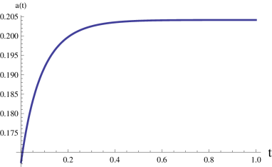
Figure 6: The scale factor for $\ell=1$, $\rho_{0}=1$ and $C_{3}=1$ in the radiation model is shown in the left figure. In the right figure the scale factor for $C_{3}=-1$ is shown.

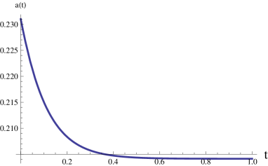
Figure 7: The scale factor for $\ell=-1$, $\rho_{0}=1$ and $C_{3}=1$ in the radiation model is shown in the left figure. In the right figure the scale factor for $C_{3}=1$ is shown. Note that since in the metric (2), $a^{2}(t)$ is appeared so the absolute value of the scale factor (23) is meaningful.

4 Canonical quantization: the WD equation

We now focus attention on the study of the quantum cosmology of the models described above. For this purpose we quantize the dynamical variables with the use of the WD equation, that is, ${\cal H}\Psi=0$, where ${\cal H}$ is the operator form of the Hamiltonian given by equation (4), and $\Psi$ is the wave function of the universe, a function of the scale factor and the matter fields, if they exist.

4.1 The de Sitter model

Let us set $V(a)=2\Lambda$. Then the corresponding WD equation becomes

$${\cal{H}}\Psi(a)=\left[\frac{1}{24}a^{-1}p_{a}^{2}-2\Lambda a^{3}\right]\Psi(a)=0.$$ (24)

Choice of the ordering $a^{-1}p_{a}^{2}=p_{a}a^{-1}p_{a}$ to make the Hamiltonian Hermitian and use of $[a,p_{a}]=i\hbar$ and $p_{a}=-i\hbar\partial_{a}$ results in

$$\partial_{a}^{2}\Psi(a)-a^{-1}\partial_{a}\Psi(a)+\frac{48\Lambda}{\hbar^{2}}a^{4}\Psi(a)=0,$$ (25)

with solutions

$$\Psi(a)=c_{1}aJ_{\frac{1}{3}}\left(\frac{4a^{3}\sqrt{\Lambda}}{\hbar\sqrt{3}}\right)+c_{2}aJ_{-\frac{1}{3}}\left(\frac{4a^{3}\sqrt{\Lambda}}{\hbar\sqrt{3}}\right),$$ (26)

where $J$ is the Bessel function and $c_{1}$ and $c_{2}$ are arbitrary constants. The constants must be so chosen as to satisfy the initial conditions. However, in what follows, our discussions are independent of the values of these constants. Here we show and emphasize the different behavior of both solutions. To do this we need to calculate the probability density $|\Psi(a)|^{2}$. In figures 8 and 9 the probability density for $c_{2}=0$ and $c_{1}=0$ are shown respectively.

Figure 8: The probability density for the $J_{\frac{1}{3}}$ term with $\Lambda=0.0001$.

Figure 9: The probability density for the $J_{-\frac{1}{3}}$ term with $\Lambda=0.0001$.

Now, we start form a chosen initial condition, say, $a=1$. The PEP procedure may now be employed to describe the physical interpretation of the resulting states. In figure 8, let the initial state be at point $P$. One then expects, keeping in mind the discussion presented previously, the transition $P{\buildrel{PEP}\over{\longrightarrow}}Q$ to appear, with the following physical interpretation. The point $P$ shows an initial state and the point $Q$ shows the final state. The universe begins its evolution by a monotonically increasing scale factor to reach the point $Q$. Point $Q$ is a state with a greater scale factor and is finite. Note that since the point $Q$ is a local maximum, PEP predicts $Q{\buildrel{PEP}\over{\longrightarrow}}Q$ which means that the scale factor remains in this final state. The transition $P{\buildrel{PEP}\over{\longrightarrow}}Q$ then means starting from an initial state, increasing monotonically, and finally arriving at a constant final state. This behavior is completely similar to the behavior of the scale factor in the previous section, presented in the left plot in figure 2.

Since for the other cases the details are similar, in the following we mention only the correspondence between the solutions without any detail. In figure 8, the transition $R{\buildrel{PEP}\over{\longrightarrow}}Q$ is similar to the right plot in figure 2. On the other hand in the same figure, transition $T{\buildrel{PEP}\over{\longrightarrow}}U$ is similar to that of the left plot in figure 2 with a different initial condition, that is, with an appropriate $C_{1}$. The transition $Q{\buildrel{PEP}\over{\longrightarrow}}Q$ represents the scale factor (17) with $C_{1}=0$. In figure 9, similar discussions as above apply and the transitions $Q{\buildrel{PEP}\over{\longrightarrow}}P$ and $T{\buildrel{PEP}\over{\longrightarrow}}S$ have the behavior and interpretation compatible with the right plot in figure 3 with different initial conditions. Again, $R{\buildrel{PEP}\over{\longrightarrow}}S$ is similar to the left plot in figure 3.

Now, an interesting question arises as to the meaning of $P{\buildrel{PEP}\over{\longrightarrow}}P$ in this case. One possible answer would be that only superpositions of the solutions are appropriate for comparison with the previous section results, e.g. $c_{1}=c_{2}=1$ and $c_{1}=-c_{2}=1$.

It is appropriate at this point to discuss different values of the final scale factor predicted by the WD equation. Obviously, since the maximum probabilities in figures 8 and 9 occur at different values then the final scale factor assumes different values too. This prediction is compatible with the deformed phase-space method due to the appearance of the lapse function, $N$, as a constant parameter in relation (17) controlling the behavior of the scale factor. It is worth mentioning that in both approaches there are two parameters that control the behavior of the scale factor; $C_{1}$ in the deformed phase-space method and also $N$ which is fixed by the maximum value of the scale factor and its initial values in each region of the WD solution. Note that each region is an interval between two minima that contains one maximum. For example in figure 6 the region containing points $P$ and $Q$ is one region and that containing $T$ and $U$ is another region and the same is true for other figures.

4.2 The dust model

In this case we set $V(a)=\rho_{0}a^{-3}$ in Hamiltonian (4). The corresponding WD equation becomes

$${\cal{H}}\Psi(a)=\left[\frac{1}{24}a^{-1}p_{a}^{2}-\rho_{0}\right]\Psi(a)=0.$$ (27)

With the above ordering, the WD equation is

$$\partial_{a}^{2}\Psi(a)-a^{-1}\partial_{a}\Psi(a)+\frac{24\rho_{0}}{\hbar^{2}}a\Psi(a)=0,$$ (28)

with solution

$$\Psi(a)=c^{\prime}_{1}\mbox{Ai}^{\prime}\left[2\left(\frac{-3\rho_{0}}{\hbar^{2}}\right)^{1/3}a\right]+c^{\prime}_{2}\mbox{Bi}^{\prime}\left[2\left(\frac{-3\rho_{0}}{\hbar^{2}}\right)^{1/3}a\right],$$ (29)

where $c^{\prime}_{1}$ and $c^{\prime}_{2}$ are integration constants and $\mbox{Ai}^{\prime}$ and $\mbox{Bi}^{\prime}$ are derivatives of the Airy functions Ai and Bi with respect to $a$ respectively. In this case the corresponding probability densities $|\Psi(a)|^{2}$ are shown in figures 10 and 11 where $c^{\prime}_{1}=0$ and $c^{\prime}_{2}=0$ respectively.

Figure 10: The probability density for the $\mbox{Bi}^{\prime}$ term with $\rho_{0}=1$.

Figure 11: The probability density for the $\mbox{Ai}^{\prime}$ term with $\rho_{0}=1$.

In the dust model two different solutions show completely different behaviors. One, figure 10, has local maxima but the other, figure 11, is monotonically increasing. In figure 10, the transition $Q{\buildrel{PEP}\over{\longrightarrow}}R$ is compatible with the left plot in figure 4. Transition $S{\buildrel{PEP}\over{\longrightarrow}}R$ however, is compatible with the right plot in figure 4 with transitions $P{\buildrel{PEP}\over{\longrightarrow}}P$ and $R{\buildrel{PEP}\over{\longrightarrow}}R$ being compatible with scale factor (19) with different initial conditions and constants.

It is worth noting that the transition $P{\buildrel{PEP}\over{\longrightarrow}}Q$ in figure 11 means that no matter what the initial state is, the scale factor moves to a larger value and continues to grow since in this case no local maximum exists at all. This behavior is completely in agreement with the behavior of the scale factor represented in figure 5. Note that a similar discussion like that of the last paragraph of the previous subsection goes for the dust case. Note that for figure 11 there is only one region.

4.3 The radiation model

In the radiation case the Hamiltonian (4) with $V(a)=\rho_{0}a^{-4}$ results in the following WD equation

$${\cal{H}}\Psi(a)=\left[\frac{1}{24}a^{-1}p_{a}^{2}-\rho_{0}a^{-1}\right]\Psi(a)=0.$$ (30)

By using the mentioned ordering it reduces to a differential equation as follow

$$\partial_{a}^{2}\Psi(a)-a^{-1}\partial_{a}\Psi(a)+\frac{24\rho_{0}}{\hbar^{2}}a\Psi(a)=0,$$ (31)

with solution

$$\Psi(a)=c^{\prime\prime}_{1}aJ_{1}\left(2\sqrt{6\hbar}a\right)+c^{\prime\prime}_{2}aY_{1}\left(2\sqrt{6\hbar}a\right),$$ (32)

where $c^{\prime\prime}_{1}$ and $c^{\prime\prime}_{2}$ are integration constants and $J$ and $Y$ are Bessel functions. The behavior of the above functions are represented in figures 12 and 13. The discussions on comparison between quantum cosmological solutions and their correspondence from deformed phase-space formalism, i.e. figure 6, are the same as previous models, cosmological constant and dust models. To prevent making the paper boring we omit discussing for this case.

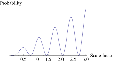
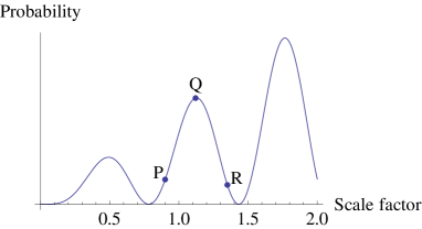
Figure 12: The probability density for the $J$-Bessel term with $\rho_{0}=1$ and $\hbar=1$.

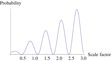
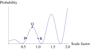
Figure 13: The probability density for the $Y$-Bessel term with $\rho_{0}=1$ and $\hbar=1$.

5 Bianchi type I Model

In this section we consider a more complicated model i.e. Bianchi model with different matter fields and compare its quantum behavior that is modeled by a kind of phase-space deformation and also canonical quantization. We separate Bianchi models from previous ones since there is more than one variable exists that makes our conjecture more reasonable.

5.1 Phase-space deformation

Let us consider a cosmological model in which the spacetime is assumed to be of Bianchi type I whose metric can be written as

$$ds^{2}=-N^{2}(t)dt^{2}+e^{2u(t)}e^{2\beta_{ij}(t)}dx^{i}dx^{j},$$ (33)

where $N(t)$ is the lapse function, $e^{u(t)}$ is the scale factor of the universe and $\beta_{ij}(t)$ determine the anisotropic parameters $v(t)$ and $w(t)$ as follows

$$\beta_{ij}=\mbox{diag}\left(v+\sqrt{3}w,v-\sqrt{3}w,-2v\right).$$ (34)

To simplify the model we take $w=0$, where is equivalent with a universe with two scale factors in the form

$$ds^{2}=-N^{2}(t)dt^{2}+a^{2}(t)(dx^{2}+dy^{2})+c^{2}(t)dz^{2}.$$ (35)

The anisotropy in the above metric can achieved by introducing a large scale homogeneous magnetic field in a flat FRW spacetime. Such a magnetic field results in a preferred direction in space along the direction of the field. If we introduce a magnetic field which has only a $z$ component, the resulting metric can be written in the form (35) where there are equal scale factors in the transverse directions $x$ and $y$ and a different one, $c(t)$, in the longitudinal direction $z$. The Hamiltonian for gravity coupled to a perfect fluid with equation of state $p=\gamma\rho$ is

$${\cal H}=\frac{1}{24}Ne^{-3u}\left(-p_{u}^{2}+p_{v}^{2}\right)+NM_{\gamma}e^{-3\gamma u}+\lambda\pi,$$ (36)

where, $M_{\gamma}$ is a model dependent constant. To introduce noncommutativity one can start with

$$\left\{N^{\prime}(t),e^{u^{\prime}+v^{\prime}}\right\}=\ell e^{u^{\prime}+v^{\prime}},\hskip 14.22636pt\left\{N^{\prime}(t),e^{u^{\prime}-2v^{\prime}}\right\}=\ell e^{u^{\prime}-2v^{\prime}},$$ (37)

where are the two dimensional generalization of relation (6). The Hamiltonian of this model becomes

$${\cal H^{\prime}}_{0}=\frac{1}{24}N^{\prime}e^{-3u^{\prime}}\left(-{p^{\prime}}_{u}^{2}+{p^{\prime}}_{v}^{2}\right)+N^{\prime}M_{\gamma}e^{-3\gamma u^{\prime}}.$$ (38)

Now we introduce as before

$$\left\{\begin{array}[]{ll}N^{\prime}(t)=N(t)-\alpha\ell p_{u}(t)-\beta\ell p_{v}(t),\\ u^{\prime}(t)=u(t),\hskip 14.22636ptv^{\prime}(t)=v(t),\\ p^{\prime}_{u}(t)=p_{u}(t),\hskip 8.5359ptp^{\prime}_{v}(t)=p_{v}(t)\end{array}\right.$$ (42)

where $\alpha+\beta=1$. The deformed Hamiltonian by imposing the above transformations takes the form

$${\cal H}^{nc}=\left[N(t)-\alpha\ell p_{u}(t)-\beta\ell p_{v}(t)\right]\left[\frac{1}{24}e^{-3u}\left(-p_{u}^{2}+p_{v}^{2}\right)+M_{\gamma}e^{-3\gamma u}\right]+\lambda\pi.$$ (43)

The classical dynamics is governed by the Hamiltonian equations, that is

$$\left\{\begin{array}[]{ll}\dot{u}=\{u,{\cal H}^{nc}\}=-\frac{1}{12}e^{-3u}p_{u}\left[N(t)-\alpha\ell p_{u}(t)-\beta\ell p_{v}(t)\right]-\alpha\ell\left[\frac{1}{24}e^{-3u}\left(-p_{u}^{2}+p_{v}^{2}\right)+M_{\gamma}e^{-3\gamma u}\right],\\ \\ \dot{v}=\{v,{\cal H}^{nc}\}=\frac{1}{12}e^{-3u}p_{v}\left[N(t)-\alpha\ell p_{u}(t)-\beta\ell p_{v}(t)\right]-\beta\ell\left[\frac{1}{24}e^{-3u}\left(-p_{u}^{2}+p_{v}^{2}\right)+M_{\gamma}e^{-3\gamma u}\right],\\ \\ \dot{p_{u}}=\{p_{u},{\cal H}^{nc}\}=\left[N(t)-\alpha\ell p_{u}(t)-\beta\ell p_{v}(t)\right]\left[-\frac{1}{8}e^{-3u}\left(-p_{u}^{2}+p_{v}^{2}\right)-3\gamma M_{\gamma}e^{-3\gamma u}\right],\\ \\ \dot{p_{v}}=\{p_{v},{\cal H}^{nc}\}=0,\\ \\ \dot{N}=\{N,{\cal H}^{nc}\}=\lambda,\\ \\ \dot{\pi}=\left\{\pi,{\cal{H}}^{nc}\right\}=\frac{1}{24}e^{-3u}\left(-p_{u}^{2}+p_{v}^{2}\right)+M_{\gamma}e^{-3\gamma u}.\end{array}\right.$$ (55)

The requirement that the primary constraints should hold during the evolution of the system means that $\dot{\pi}=\left\{\pi,{\cal H}^{nc}\right\}=0$. Applying this condition into the above equations we get

$$\left\{\begin{array}[]{ll}\dot{u}=-\frac{1}{12}e^{-3u}p_{u}\left[N-\alpha\ell p_{u}(t)-\beta\ell p_{0v}\right],\\ \\ \dot{v}=\frac{1}{12}e^{-3u}p_{v}\left[N-\alpha\ell p_{u}(t)-\beta\ell p_{0v}\right],\\ \\ \dot{p_{u}}=-3(\gamma-1)M_{\gamma}e^{-3\gamma u}\left[N-\alpha\ell p_{u}(t)-\beta\ell p_{0v}\right].\end{array}\right.$$ (61)

Since the analytic solution does not exist for the above equations, their behavior is represented in figures 14 and 15 by applying numerical methods. In figure 14 for $u$, there is a decreasing era before steady behavior in contrast to $v$-behavior. However, the other choices are possible too. For example, in figure 15, both of $u$ and $v$ are the same in the existence of a decreasing era in their behaviors. These figures are plotted for typical numerical values for the parameters and initial conditions. With examining some other initial conditions the behavior is almost repeated.

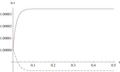
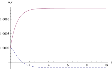
Figure 14: Left plot is shown for $\gamma=-1$ (de Sitter) and right one for $\gamma=0$ (dust). We take $\alpha=\beta=1/2$, $p_{0v}=1$, $N=1$, $\ell=1$, $M_{\gamma}=1$ and initial conditions $u(t=0)=v(t=0)=1$, $p_{u}(t=0)=0$. The dashed lines represent $u$-behavior and the solid line $v$-behavior in both figures.

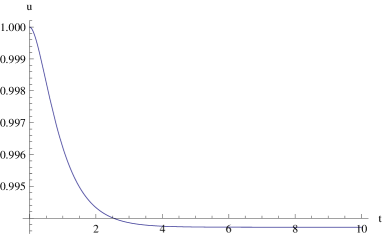
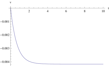
Figure 15: This figures are sketched only for dust, $\gamma=0$. We take $\alpha=\beta=1/2$, $p_{0v}=-1$, $N=1$, $\ell=1$, $M_{\gamma}=1$ and initial conditions $u(t=0)=v(t=0)=1$, $p_{u}(t=0)=0$. In the left plot $u$-behavior is represented and $v$-behavior is represented in the right one.

5.2 Canonical quantization

The WD equation for our model reads

$${\cal H}\Psi(u,v)=0\Rightarrow\left[\frac{\partial^{2}}{\partial u^{2}}-\frac{\partial^{2}}{\partial v^{2}}+24M_{\gamma}e^{3(1-\gamma)u}\right]\Psi(u,v)=0.$$ (62)

The solutions to the above equation are

$$\Psi_{\nu}(u,v)=e^{\pm i\nu v}J_{\pm i\nu/3}(4\sqrt{\frac{M_{\gamma}}{6}}e^{3u}),$$ (63)

for $\gamma=-1$ and

$$\Psi_{\nu}(u,v)=e^{\pm i\nu v}J_{\pm 2i\nu/3}(4\sqrt{\frac{2M_{\gamma}}{3}}e^{3u/2}),$$ (64)

for $\gamma=0$, where $\nu$ is a separation constant. We have chosen oscillatory function $e^{\pm i\nu v}$ since the real exponents would lead to exponential increasing wave function for $v\rightarrow\pm\infty$ that would not show physical behavior. Therefore, we may now write the general solution of the WD equation as a superposition of the above eigenfunctions

$$\Psi(u,v)=\int_{-\infty}^{+\infty}C(\nu)\Psi_{\nu}(u,v)d\nu,$$ (65)

where $C(\nu)$ can be chosen as a shifted Gaussian weight function $e^{-a(\nu-b)^{2}}$. The square of wave function for different cases are shown in figures 16 and 17 for de Sitter case and dust respectively.

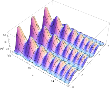
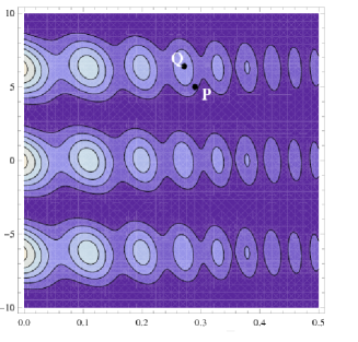
Figure 16: The right plot is shown $|\Psi(u,v)|^{2}$ and the left is its corresponding contour plot. It is for de Sitter case with $M_{\gamma}=20$. It is taken only two first terms of relation (65) with a constant wight function.

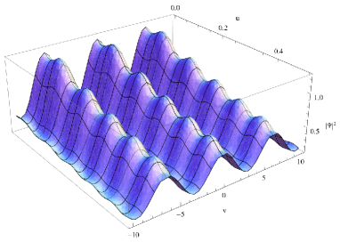
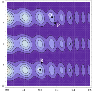
Figure 17: The right plot is shown $|\Psi(u,v)|^{2}$ and the left is its corresponding contour plot. It is for dust with $M_{\gamma}=20$. It is taken only two first terms of relation (65) with a constant wight function.

In figure 16 point $Q$ is located at a local maximum probability so PEP predicts a transition from point $P$ to $Q$ i.e. $P{\buildrel{PEP}\over{\longrightarrow}}Q$. Physically, this transition imposes going $u$ down and going $v$ up and after $P{\buildrel{PEP}\over{\longrightarrow}}Q$ since $Q$ is located at a maximum then $Q{\buildrel{PEP}\over{\longrightarrow}}Q$ that means the system be steady at $Q$. This behavior is exactly similar to previous result which is represented in the left plot in figure 14. The similar is true for the left plot in figure 14 and $P{\buildrel{PEP}\over{\longrightarrow}}Q$ transition in figure 17. Since point $S$ is located at a local maximum probability so PEP predicts $R{\buildrel{PEP}\over{\longrightarrow}}S$ then $S{\buildrel{PEP}\over{\longrightarrow}}S$. It means there is this possibility that both of $u$ and $v$ go down. This later result is completely in agreement with the previous subsection results i.e. the represented case in figure 15.

There is a notable difference between Bianchi model and previous ones that is existence of more than one direction in configuration space for Bianchi model. This makes some ambiguities in path of transition to more probable state in PEP paradigm. But as mentioned roughly in [10] the path in these kinds of examples is on the gradient of $|\Psi|^{2}$ (hyper-)surface which has the most slope. This proposal results in definition of a unique transition path in PEP for more complicated configuration spaces.

6 Discussion

In this paper we have argued, using familiar examples, that one can draw a completely equivalent physical interpretation for two different approaches to quantization, namely the usual canonical quantization method and the phase-space deformation method, at least within the framework of the examples used in this work. A by-product is that when one studies the deformation of phase-space, one should realize that this is effectively a quantization procedure and should refrain from using any other quantization method simultaneously. However, since in the phase-space deformation method for quantization the evolutionary parameter, $t$, does appear, in contrast to the canonical method, a mechanism for retrieving the dynamical information of the system, when canonically quantized, is at hand and can be used. This had been done in a previous work [10, 11]. The results show that if the equivalence of different methods of quantization discussed above are assumed, then the probabilistic evolutionary mechanism works consistently and therefore can be used to address the problem of evolution in diffeomorphism invariant theories.

However, such an equivalence cannot hold true in examples where the deformation in phase-space is introduced in a Lorentz non-invariant manner. This is not hard to predict since the WD equation is a direct result of diffeomorphism invariance and so if a deformation in phase-space breaks such an invariance then the results of different quantization methods should be different. In this connection we note that $\kappa$-Minkowski deformation and GUP, for example, preserve Lorentz invariance [24].

Another feature which is of interest is that the WD equation is usually a second order differential equation and has therefore two independent solutions. However, in the deformed phase-space quantum models, the equations of motion are first order, in contrast to the former. The disparity lies in the fact that, as discussed above, the parameter of deformation, $\ell$, is arbitrary, and hence can be chosen to be either positive or negative. It has been shown that different signs of $\ell$ relate to different solutions of the WD equation.

It is worth mentioning that this paper can be read as a companion for our previous one [10]. In [10] we have discussed on the PEP paradigm massively but here to make the current manuscript self-studied we highlight some crucial features of PEP very rapidly. The PEP proposal has some roots in the second law of thermodynamics that is a system in an initial state evolves approaching to another state in which the final state has a more entropy value or a same one i.e. $S_{f}-S_{i}=\bigtriangleup S\geq 0$. A vital problem in PEP is the velocity of transition from a state to a more probable state. Actually, this question has not any concrete answer yet due to the first steps in understanding PEP. But in a model discussed in [10] there is a relation for the velocity of transition what is achieved by comparison of PEP’s results with Causal Dynamical Triangulation method as a model of quantum gravity. It means until now it is an open problem that how the velocity of transition can be addressed by PEP itself.

Finally, it is significant to consider that if a proposal is correct in few examples it does not mean its correctness universally and in this paper it is not our claim in any senses. But we have shown that there is a kind of correspondence between different methods of quantizations. We suppose, at least, this correspondence should be considered until a complete understanding of the universe. Since in lack of a full theory, e.g. quantum gravity, all the approaches are considerable and perhaps each approaches sheds some lights on various parts of the universe. This viewpoint results in a proposal that a combination of different approaches is a part of full theory. However, maybe, different approaches have an intersection in their territory of validness that have to be characterized exactly to do not result in double consideration, e.g. double calculations. In this paper we have shown that two different methods of quantizations can be same as each other at least in some specific examples and it must be considered to prevent double quantization. And even more this correspondence can shed lights by each methods on the other methods for example it can be interpreted as an evidence for correctness of PEP method as a developing in understanding canonical quantization method.

References

- [1] B.S. DeWitt, Phys. Rev. 160 (1967) 1113
- [2] C.W. Misner, Phys. Rev. 186 (1969) 1319
-
[3]
A. Vilenkin, Phys. Lett. B 117 (1982) 25
A. Vilenkin, Phys. Rev. D 27 (1983) 2848
A. Vilenkin, Phys. Rev. D 33 (1986) 3560
A. Vilenkin, Phys. Rev. D 37 (1988) 888
A. Vilenkin, Phys. Rev. D 50 (1994) 2581
J.B. Hartle and S.W. Hawking, Phys. Rev. D 28 (1983) 2960
S.W. Hawking, Nucl. Phys. B 239 (1984) 257
J.J. Halliwell and S.W. Hawking, Phys. Rev. D 31 (1985) 1777
G.W. Gibbons and J.B. Hartle, Phys. Rev. D 42 (1990) 2458 - [4] D.L. Wiltshire, An Introduction to Quantum Cosmology, (arXiv: gr-qc/0101003)
-
[5]
M.P. Ryan, Hamiltonian Cosmology, Springer, Berlin (1972)
M.P. Ryan and L.C. Shepley, Homogeneous Relativistic Cosmologies, Princeton University Press, Princeton (1975) - [6] C.J. Isham, Canonical quantum gravity and the problem of time, lectures presented at NATO Advanced Study Institute, Salamanca, (1992) (arXiv: gr-qc/9210011)
- [7] W.F. Blyth and C.J. Isham, Phys. Rev. D 11 (1975) 768
- [8] B. Vakili and H.R. Sepangi, Ann. Phys. 323 (2008) 548 (arXiv:0709.2988[gr-qc] )
- [9] C. K. Zachos, D. B. Fairlie and T. L. Curtright (editors), Quantum Mechanics in Phase Space, World Scientific Publishing Co. (2005)
- [10] N. Khosravi and H. R. Sepangi, Phys. Lett. B 673 (2009) 297 (arXiv: 0903.1914)
- [11] N. Khosravi, S. Jalalzadeh and H.R. Sepangi, Gen. Rel. Grav. 39 (2007) 899 (arXiv: gr-qc/0702067)
- [12] N. Khosravi and H.R. Sepangi, J. Cosmol. Astropart. Phys. JCAP04 (2008) 011 (arXiv: 0803.1714[gr-qc])
- [13] N. Khosravi and H.R. Sepangi, Phys. Lett. A 372 (2008) 3356 (arXiv: 0802.0767 [gr-qc])
-
[14]
J.J. Halliwell, The Interpretation of Quantum Cosmology and the Problem of Time,
(arXiv: gr-qc/0208018)
J.J. Halliwell The Interpretation of Quantum Cosmological Models, (arXiv: gr-qc/9208001) -
[15]
H. Garcia-Compean, O. Obregon and C. Ramirez, Phys.
Rev. Lett. 88 (2002) 161301 (arXiv: hep-th/0107250)
J.C. Lopez-Dominguez, O. Obregon, C. Ramirez and M. Sabido, Phys. Rev. D 74 (2006) 084024 (arXiv: hep-th/0607002)
G.D. Barbosa and N. Pinto-Neto, Phys. Rev. D 70 (2004) 103512 (arXiv: hep-th/0407111)
N. Khosravi, S. Jalalzadeh and H.R. Sepangi, J. High Energy Phys. JHEP 01 (2006) 134, (arXiv: hep-th/0601116)
B. Vakili, N. Khosravi and H.R. Sepangi, Class. Quantum Grav. 24 (2007) 931 (arXiv: gr-qc/0701075) - [16] L.J. Garay, Int. J. Mod. Phys. A 10 (1995) 145 (arXiv: gr-qc/9403008)
-
[17]
A. Connes, Noncommutative geometry, Academic Press
(1994)
A. Connes, J. Math. Phys. 41 (2000) 3832 (arXiv: hep-th/0003006)
S. Majid, Lect. Notes Phys. 541 (2000) 227 (arXiv: hep-th/0006166) - [18] A. Kempf, G. Mangano and R.B. Mann, Phys. Rev. D 52 (1995) 1108 (arXiv: hep-th/9412167)
-
[19]
J.M. Carmona, J. L. Cortes, J. Gamboa and F.
Mendez, J. High Energy Phys. JHEP 03 (2003) 058
(arXiv: hep-th/0301248)
J.M. Carmona, J.L. Cortes, J. Gamboa and F. Mendez, Phys. Lett. B 565 (2003) 222 (arXiv: hep-th/0207158) -
[20]
S.M. Carroll, J.A. Harvey, V.A. Kostelesky, C.D. Lane and T.
Okamoto, Phys. Rev. Lett. 87 (2001) 141601 (arXiv:
hep-th/0105082)
C.E. Carlson, C.D. Carone and R.F. Lebed, Phys. Lett. B 518 (2001) 201 (arXiv: hep-ph/0107291)
C.E. Carlson, C.D. Carone and R.F. Lebed, Phys. Lett. B 549 (2002) 337 (arXiv: hep-ph/0209077) -
[21]
B. Vakili and H.R. Sepangi, Phys. Lett. B 651 (2007) 79 (arXiv: 0706.0273
[gr-qc])
B. Vakili, Phys. Rev. D 77 (2008) 044023 (arXiv: 0801.2438[gr-qc])
M.V. Battisti and G. Montani, Phys. Lett. B 656 (2007) 96 (arXiv: gr-qc/0703025)
M.V. Battisti and G. Montani, Phys. Rev. D 77 (2008) 023518 (0707.2726 [gr-qc])
H.R. Sepangi, B. Shakerin and B. Vakili, Class. Quantum Grav. 26 (2009) 065003 (arXiv: 0901.3829 [gr-qc])
B. Vakili, Int. J. Mod. Phys. D 18 (2009) 1059 (arXiv: 0811.3481 [gr-qc]) -
[22]
G. Amelino-Camelia, Int. J. Mod. Phys. D 11 (2002) 1643 (arXiv: gr-qc/0210063)
J. Kowalski-Glikman, Introduction to Doubly Special Relativity, Lect. Notes Phys. 669 (2005) 131 (arXiv: hep-th/0405273)
G. Amelino-Camelia, Int. J. Mod. Phys. D 11 (2002) 35 (arXiv: gr-qc/0012051)
G. Amelino-Camelia, Phys. Lett. B 510 (2001) 255 (arXiv: hep-th/0012238)
J. Magueijo and L. Smolin, Phys. Rev. Lett. 88 (2002) 190403 (arXiv: hep-th/0112090)
J. Kowalski-Glikman and S. Nowak, Phys. Lett. B 539 (2002) 126 (arXiv: hep-th/0203040)
J. Lukierski, A. Nowicki, H. Ruegg and V. N. Tolstoy, Phys. Lett. B 268 (1991) 331 - [23] J. Kowalski-Glikman, Phys. Lett. A 299 (2002) 454 (arXiv: hep-th/0111110)
- [24] J.M. Romero, J.D. Vergara and J.A. Santiago, Phys. Rev. D 75 (2007) 065008 (arXiv: hep-th/0702113)
-
[25]
J. Lukierski, A. Nowicki and H. Ruegg, Phys. Lett. B 293 (1992)
344
S. Majid and H. Ruegg, Phys. Lett. B 334 (1994) 348 (arXiv: hep-th/9405107) - [26] L. Freidel, J. Kowalski-Glikman and S. Nowak, Phys. Lett. B 648 (2007) 70 (arXiv: hep-th/0612170)
- [27] N.R. Bruno, G. Amelino-Camelia and J. Kowalski-Glikman, Phys. Lett. B 522 (2001) 133 (arXiv: hep-th/0107039)
- [28] N. Khosravi, H.R. Sepangi and M.M. Sheikh-Jabbari, Phys. Lett. B 647 (2007) 219 (arXiv: hep-th/0611236)
- [29] M. Chaichian, M.M. Sheikh-Jabbari and A. Tureanu, Phys. Rev. Lett. 86 (2001) 2716 (arXiv: hep-th/0010175)
- [30] J.R. Nascimento, A. Yu. Petrov and R.F. Ribeiro, Europhys. Lett. 77 (2007) 51001 (arXiv: hep-th/0601077)