I Introduction

This paper is the second part of a study of the scale-locality properties of the energy cascade of three-dimensional turbulence. In the first part EyinkAluie (hereafter referred to as I) we investigated energy transfer defined by means of low-pass and band-pass filters for smooth, dilated kernels, which permit simultaneous resolution of the physical processes both in space and in scale. We demonstrated there the scale-locality of interactions involved in turbulent energy transfer, by rigorous analysis and by numerical simulation. See also Eyink95a , Eyink05 . The discussion in these papers did not apply to sharp-spectral filters, which do not satisfy the modest decay conditions in physical space that were employed there. The origin of scale-locality with the sharp spectral filter is, in fact, a rather more subtle issue. The problem is of importance, however, since most numerical studies of turbulent scale-locality employ sharp spectral filters. We believe that misinterpretation of the numerical results has led to a number of misunderstandings in the literature.

Early papers on turbulent energy cascade which employed spectral analysis—such as those of Obukhov Obukhov41a , Obukhov41b , Onsager Onsager45 , Onsager49 , and Heisenberg Heisenberg48 —argued for scale-locality. Those works proposed a “cascade process” in which two modes of similar wavenumber transfer energy to a mode with twice that wavenumber, implying steps in spectral space of increasing size with increasing wavenumber. This picture was later confirmed by detailed closure calculations of Kraichnan, both for his (Eulerian) direct-interaction approximation (DIA) Kraichnan59 , his abridged Lagrangian-history direct-interaction approximation (ALHDIA) Kraichnan66 , and the test-field model (TFM) Kraichnan71a . In the late 80’s and early 90’s, however, this traditional view was contested in numerical simulation studies by a number of authors: Brasseur & Corrsin BrasseurCorrsin , Domaradzki & Rogallo DomaradzkiRogallo , Yeung & Brasseur YeungBrasseur , and Ohkitani & Kida OhkitaniKida . Those works presented results suggesting that energy cascade is dominated by highly nonlocal triadic interactions, with one very energetic mode at the lowest wavenumber $k_{0}$ catalyzing transfer between two modes at high wavenumbers $k<k^{\prime},$ for $k^{\prime}-k=O(k_{0}).$ This transfer process was described as “local transfer through nonlocal interactions”. In contrast to the traditional picture, the energy flow through spectral space was suggested to proceed via steps of a fixed, small size $k_{0},$ driven by low-wavenumber advection. Chasnov Chasnov91 argued that such nonlocal, advective sweeping interactions should be incorporated into spectral large-eddy simulation (LES) via a stochastic force that produces random backscatter of energy. If such views were correct, they would present a fundamental challenge to the Kolmogorov picture of local energy cascade and the universality of small-scale turbulence.

Several theoretical papers published shortly thereafter defended the traditional view of turbulent scale-locality LvovFalkovich , Waleffe92 , Zhou93a , Zhou93b , Eyink94 . In particular, Waleffe Waleffe92 , Zhou Zhou93a , Zhou93b and Eyink Eyink94 all argued that scale-locality is recovered when Fourier modes are suitably combined or averaged. Zhou Zhou93a , Zhou93b showed numerically that locality does hold, when some necessary summations are made, and he verified the quantitative prediction of Kraichnan Kraichnan66 , Kraichnan71 that non-local contributions to energy flux decay as a power $\propto s^{4/3}$ of the “scale-disparity parameter” $s=k_{\min}/k_{{\rm med}}$ (where $k_{\max},k_{{\rm med}},k_{\min}$ are the maximum, median, and minimum wavenumbers of a triad, respectively). It seems, however, that this conclusion was subjected to doubt in a subsequent investigation by Zhou et al. (1996) Zhouetal96 which indicated that the effects of the largest scales are significant. The paper of Eyink (1994)Eyink94 proved rigorously that spectral energy flux, if averaged in wavenumber over an octave band, is dominated by local triads. His argument yielded a rigorous upper bound $O(s^{2/3})$ on the nonlocal triadic contributions, which is larger than Kraichnan’s scaling prediction but still vanishing as $s\rightarrow 0$. However, the paper of Eyink also proved that the spectral energy flux, without additional averaging, may be non-local. He constructed a velocity field with Hölder continuity properties analogous to those observed in turbulent flow for which the instantaneous spectral energy flux is dominated by nonlocal advective interactions, somewhat similar to the effects seen in the numerical simulations BrasseurCorrsin , DomaradzkiRogallo , YeungBrasseur , OhkitaniKida .

The debate about the locality of interactions contributing to energy flux with the sharp spectral filter has continued unabated. Recently, the issue was addressed by numerical simulations at much higher Reynolds numbers by Alexakis et al. (2005) Alexakisetal05b and Mininni et al. (2006,2008) Mininni06 , Mininni08 , who concluded, in agreement with the earlier simulations BrasseurCorrsin , DomaradzkiRogallo , YeungBrasseur , OhkitaniKida , that the important interactions contributing to interband transfers are those among highly non-local wavenumber triads with one leg at the energy peak. On the other hand, they concluded that the spectral energy flux, involving a suitable summation of Fourier modes, is dominated by local triads. Domaradzki & Carati (2007,2009) Domaradzki07b , Domaradzki09 confirmed these results and furthermore numerically calculated Kraichnan’s Kraichnan66 , Kraichnan71 locality function $W(s),$ a quantity which measures the fractional contribution of nonlocal triads. They verified Kraichnan’s prediction that $W(s)\propto s^{4/3}$ for $s\ll 1,$ in agreement with earlier studies of Zhou Zhou93a , Zhou93b . On the other hand, they found no difference between the sharp spectral filter and various graded filters, in apparent contradiction with the analytical work of EyinkEyink94 , Eyink95 , Eyink05 who drew a clear distinction between the sharp spectral filter and smooth, dilated filters.

It may be an understatement to say that no coherent picture of the scale-locality of turbulent energy cascade is presented by the current literature on the subject. Open issues that continue to be discussed include: the need for additional averaging (over space,time, ensembles,etc.), qualitative distinctions between sharp spectral versus smoothly graded filters, the quantitative fraction of energy flux contributed by non-local triads, and possible differences between spectral binning with logarithmic versus linear bands. Even the proper definition of “energy flux” is unclear, since the definition used in the rigorous proofs with graded filters Eyink95 , Eyink05 , EyinkAluie is the “SGS flux” familiar from large-eddy simulation modeling, which involves additional advective subtractions to define the subscale stress which are not present in the conventional definition of the spectral energy flux.

The present paper has two main purposes. Our first goal is to present new results on scale-locality of spectral transfer quantities, including rigorous estimates, physical arguments and numerical simulation data. In particular, we shall show rigorously that both energy flux and inter-band transfers defined by the sharp spectral filter—without any additional averaging—are dominated by local triadic interactions. Our proof of locality rests on four ingredients: (1) The SGS flux (defined in I and in the next section) as the unique Galilean invariant measure of the inter-scale energy transfer at each point in the flow, (2) scaling properties that are observed empirically to hold for the turbulent velocity field, (3) wavenumber conservation, which constrains the number of Fourier modes contributing to the energy flux, and (4) the essential use of “logarithmic” spectral bands whose width increases proportional to wavenumber. The second aim of this paper is to attempt to collect the disparate results in the literature into a clear and consistent picture of the local cascade process in three-dimensional turbulence. We shall try to provide answers to many of the open issues mentioned above which continue to be debated in the literature.

To aid this latter goal, it may be useful to summarize here the essential reason for the dominance of local triadic interactions in energy cascade. It is true, as indicated by numerical studies BrasseurCorrsin , DomaradzkiRogallo , YeungBrasseur , OhkitaniKida , Alexakisetal05b , Mininni06 , Mininni08 , that individual non-local triads make a much bigger contribution to energy flux than individual local ones, due simply to their having one of their modes at the energy containing scales. However, such comparisons of single triads vastly underestimate the aggregate contribution from local triads. Whereas the number of highly elongated, nonlocal triads grows moderately with increasing wavenumber, the number of local triads increases much more rapidly. The net contribution to energy flux from the exploding population of local triads dwarfs the contribution from the smaller number of nonlocal triads. While this paper was being written, we discovered a work of Verma et al.Vermaetal which arrives at essentially the same conclusion, by means of a non-rigorous perturbative closure analysis of energy transfer. They stated there that “…the shell-to-shell energy transfer rate is found to be local and forward. This result is due to the fact that the nonlocal triads occupy much less Fourier space volume than the local ones.” A related observation was also made by Alexakis et al.Alexakisetal05b , who observed that the fractional contribution of non-local triads to energy flux is reduced “since many more local triads contribute in the global summation.” In fact, these ideas, as we shall discuss, are already implicit in the arguments advanced by Kraichnan for scale-locality, using his ALHDIA and TFM closuresKraichnan66 , Kraichnan71 . Our work supports these conclusions and extends them, by rigorously bounding the nonlocal contributions to spectral flux, without any heuristic approximations. Our analysis implies as well the dominance of local triads to inter-band energy transfers, for wavenumber bands of constant width on a logarithmic scale. We also explain by physical arguments how decorrelation effects (as discussed in I for the graded filter) further diminish the nonlocal contributions, giving agreement with Kraichnan’s asymptotic scaling predictions.

We verify our theoretical analysis by analyzing the velocity field ${\bf u}$ generated from a direct numerical simulation of the incompressible Navier Stokes equation

$$\partial_{t}{\bf u}+({\bf u}\cdot{\mbox{\boldmath$\nabla$}}){\bf u}=-{\mbox{\boldmath$\nabla$}}p+\nu\nabla^{2}{\bf u}+{\bf f}$$ (1)

$${\mbox{\boldmath$\nabla$}}\cdot{\bf u}=0$$

which is solved pseudo-spectrally in a periodic box of $512^{3}$ grid-points. Here, $p$ is the pressure, $\nu$ is the viscosity, and ${\bf f}$ is an external stirring force. We advance in time using the second-order Adam-Bashforth scheme and employ the phase-shift method to remove aliasing effects PattersonOrszag . The fluid is stirred using Taylor-Green forcing:

$${\bf f}\equiv f_{0}[\sin(k_{f}x)\cos(k_{f}y)\cos(k_{f}z){\hat{\bf x}}-\cos(k_{f}x)\sin(k_{f}y)\cos(k_{f}z){\hat{\bf y}}]$$ (2)

where $f_{0}=2$ is the force amplitude, and $k_{f}=2$. The viscosity $\nu$ is $0.87\times 10^{-3}$ and the Reynolds number $Re\equiv u_{rms}L/\nu\approx 11800$, where $L=2\pi$ is the size of the simulation box and $u_{rms}=\sqrt{2E_{tot}}=1.63$ is the rms velocity. The Reynold’s number based on the Taylor scale $\lambda=2\pi\sqrt{E_{tot}}/\big{(}\int dkk^{2}E(k)\big{)}^{1/2}$ is $Re_{\lambda}=615$. We analyze a time snapshot of the flow after it has reached a statistically steady state. The energy spectrum $E(k)$ of the flow, shown in Figure 1, has a reasonable $k^{-5/3}$ scaling until around $k=40$, before dissipation effects start to dominate. The mean energy flux $\overline{\Pi}_{K}=\langle\Pi_{K}\rangle$ is shown in Figure 2.

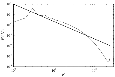
Figure 1: Energy spectrum for the simulation being analyzed. The forcing is at $k_{f}=2$. A straight line with slope $-5/3$ is added for reference.

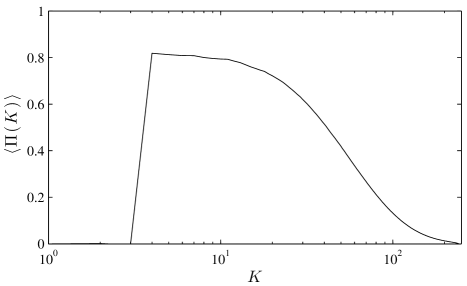
Figure 2: Average energy flux $\langle\Pi_{K}\rangle$ from the simulation.

The outline of our paper is as follows. Our main new results are presented in the following Section II. Subsection II.A contains some preliminary definitions and discussion. In subsection II.B we establish ultraviolet locality of spectral SGS flux, and in subsection II.C we establish infrared locality. In the next section III, we examine how our work relates to previous research on scale-locality, in particular the analysis of KraichnanKraichnan66 using spectral closure and recent numerical studiesAlexakisetal05b , Mininni06 , Domaradzki07a , Domaradzki07b , Mininni08 , Domaradzki09 . Section IV formulates our final conclusions.Two appendices contain some technical material, Appendix A on our rigorous proofs and Appendix B on Kraichnan’s ALHDIA closure.

II Main Analytical and Numerical Results

A Preliminaries

In a periodic domain ${\mathbb{T}}^{3}=[0,2\pi)^{3}$, one may represent a velocity field ${\bf u}$ by its Fourier series expansion:

$${\bf u}({\bf x})=\sum_{{\bf k}\in{\mathbb{Z}}^{3}}\widehat{{\bf u}}({\bf k})e^{i{\bf k}{\mbox{\boldmath$\cdot$}}{\bf x}}.$$

Restricting this sum to wavenumbers satisfying $|{\bf k}|\leq K$ yields the low-pass filtered field ${\bf u}^{<K}$, while restricting the sum to $|{\bf k}|>K$ gives the complementary high-pass filtered field ${\bf u}^{>K}={\bf u}-{\bf u}^{<K}$. We shall also employ in our discussion band-pass filtered fields

$${\bf u}^{[K,Q]}={\bf u}^{>K}-{\bf u}^{>Q}={\bf u}^{<Q}-{\bf u}^{<K}$$

for $K<Q.$ We employ a special notation $[K]$ for dyadic (octave) bands $[K/2,K]$ and denote the corresponding band-pass velocity field by ${\bf u}^{[K]}.$ The reader may assume here that $|{\bf k}|$ denotes the Euclidean norm $|{\bf k}|=\sqrt{k_{x}^{2}+k_{y}^{2}+k_{z}^{2}}$. In fact, due to very subtle aspects of harmonic analysis, our proofs do not apply with full rigor for the Euclidean norm, although they are rigorous for the norms $|{\bf k}|_{1}=|k_{x}|+|k_{y}|+|k_{z}|$ or $|{\bf k}|_{\infty}=\max\{|k_{x}|,|k_{y}|,|k_{z}|\}.$ See Appendix A for a careful discussion of these delicate mathematical issues. In fact, we believe that our arguments do apply with the Euclidean norm on wavenumbers and that the abstract mathematical counterexamples that compromise their rigor have different properties from those enjoyed by the turbulent velocity fields. In support of this belief, all of the numerical results presented later shall employ the Euclidean norm and, as may be seen, they agree with our theoretical analysis.

Just as with any other filtering scheme, one may employ the sharp spectral filter to decompose the Navier-Stokes equation (1) into large-scale and small-scale components and then consider the corresponding energy balances. Following a standard analysis, presented in I, one arrives at the sub-grid scale (SGS) energy flux

$$\Pi_{K}({\bf u},{\bf v},{\bf w})\equiv-\partial_{i}u_{j}^{<K}\bigg{(}(v_{i}w_{j})^{<K}-v_{i}^{<K}w_{j}^{<K}\bigg{)}$$ (3)

as the representation of the transfer rate of energy from modes with wavenumbers $<K$ to modes with wavenumbers $>K$ at each space point. We have distinguished here a straining mode ${\bf u},$ an advecting mode ${\bf v},$ and an advected mode ${\bf w},$ although, in the physical balance equation, ${\bf u}={\bf v}={\bf w}.$ This permits us to formulate the property of scale-locality in a precise manner. As in I, we say that energy flux is ultraviolet (UV) scale-local if replacing any single ${\bf u}$ or any combination of ${\bf u}$’s in $\Pi_{K}({\bf u},{\bf u},{\bf u})$ by ${\bf u}^{[P]}$ gives an asymptotically negligible contribution for $P\gg K.$ Likewise, we say that energy flux is infrared (IR) scale-local if replacing any single ${\bf u}$ or any combination of ${\bf u}$’s in $\Pi_{K}({\bf u},{\bf u},{\bf u})$ by ${\bf u}^{[Q]}$ gives an asymptotically negligible contribution for $Q\ll K.$

Most of the previous studies of scale-locality with the sharp spectral filter have employed what we call an “unsubtracted flux”

$$\Pi^{uns}_{K}=-(\partial_{i}u_{j})^{<K}(u_{i}u_{j})\,\,\,\,\,{\rm or}\,\,\,\,\,-(\partial_{i}u_{j})^{<K}(u_{i}u_{j})^{<K}.$$

These two quantities have the same average over space as the SGS energy flux, because the sweeping terms which distinguish them integrate to zero: $\int d{\bf x}~{}\partial_{i}u_{j}^{<K}u_{i}^{<K}u_{j}^{<K}=0$. However, the pointwise values are different and the locality properties are different as well. Note that the quantities $\Pi_{K}({\bf u},{\bf u},{\bf u}^{[Q]})$ and $\Pi^{uns}_{K}({\bf u},{\bf u},{\bf u}^{[Q]})=-\partial_{i}u_{j}^{<K}\big{(}u_{i}u^{[Q]}_{j}\big{)}^{<K}$ are not the same even after space-averaging, since the sweeping effects no longer integrate to zero: $\int d{\bf x}~{}\partial_{i}u_{j}^{<K}u_{i}^{<K}(u^{[Q]}_{j})^{<K}\neq 0$, as was recognized by Domaradzki and Carati Domaradzki07a . Indeed, it is easy to see that the quantity $\Pi^{uns}_{K}$ cannot be scale-local instantaneously, at each point in the space domain. If we boost the flow with a uniform velocity ${\bf u}_{0}$ (a $k=0$ mode), then $\Pi^{uns}_{K}$ will develop a contribution directly proportional to this velocity. Since ${\bf u}_{0}$ can be made arbitrarily large, triads involving the $k=0$ mode can give the dominant contribution at any fixed $K$. This argument does not apply to the space (or ensemble) average of $\Pi^{uns}_{K}$, which is Galilei invariant. As we shall discuss later, the mean value $\overline{\Pi}^{uns}_{K}$ is in fact scale-local, as concluded by early workers Obukhov41a , Obukhov41b , Onsager49 , Heisenberg48 , Kraichnan59 , Kraichnan66 , although its locality properties are less robust than those of the SGS flux $\Pi_{K}.$ We examine only the latter for all of our detailed estimates in this section, and we return to discuss $\Pi^{uns}_{K}$ in section III.

Scale-locality of interactions is not a general property of solutions of the Navier-Stokes equation, e.g. the nonlinear interactions in laminar flow are dominated by the most energetic modes. Rather, the locality of the energy cascade in a turbulent flow depends crucially on some scaling properties of the solution. The operative scaling laws for sharp-spectral filtered quantities are closely related to those for velocity increments $\delta{\bf u}({\mbox{\boldmath$\ell$}};{\bf x})={\bf u}({\bf x}+{\mbox{\boldmath$\ell$}})-{\bf u}({\bf x}).$ Heuristically,

$${\bf u}^{>K}\simeq{\bf u}^{[K]}\simeq\delta u(\ell_{K}),\,\,\,\,\,\,\,{\mbox{\boldmath$\nabla$}}{\bf u}^{<K}\simeq\delta u(\ell_{K})/\ell_{K}$$

with $\ell_{K}=2\pi/K$ the length-scale corresponding to wavenumber $K.$ More precisely, the scaling laws that are used in our arguments below are for volume-averages:

$$\langle\big{|}{\bf u}^{>K}\big{|}^{p}\rangle^{1/p},\langle\big{|}{\bf u}^{[K]}\big{|}^{p}\rangle^{1/p}\sim({\rm const.})u_{rms}(KL)^{-\sigma_{p}},\,\,\,\,\langle\big{|}{\mbox{\boldmath$\nabla$}}{\bf u}^{<K}\big{|}^{p}\rangle^{1/p}\sim({\rm const.})\frac{u_{rms}}{L}(KL)^{{\color[rgb]{0,0,0}1-\sigma_{p}}}$$ (4)

with $0<\sigma_{p}<1$ and $p\geq 1,$ for inertial-range wavenumbers $K$ satisfying $KL\gg 1.$ Here $L$ is the integral length-scale, $u_{rms}$ is the root-mean-square velocity, and $\langle.\rangle$ is a volume average. Note that $\sigma_{p}=\zeta_{p}/p,$ where $\zeta_{p}$ is the scaling exponent of the $p$th-order absolute velocity structure function: $\langle[\delta u(\ell)]^{p}\rangle\sim\ell^{\zeta_{p}}$. The ultimate source of these scaling properties is empirical evidence from experiments and numerical simulations Anselmetetal , Chenetal , Sreenivasanetal . The precise mathematical forms of the scaling laws (4) that are used in our proofs are discussed in Appendix A. Here we emphasize just one salient point: the scaling law stated for $\langle\big{|}{\bf u}^{[K]}\big{|}^{p}\rangle^{1/p}$ in (4) is valid only for logarithmic bands $[K]$ and does not hold for a band $[K,K+\Delta]$ with fixed spectral width $\Delta.$ This point is essential for the proof of infrared locality, as we shall see.

B Ultraviolet Locality

We shall begin by treating the case of ultraviolet locality, which is somewhat easier and allows us to introduce the basic method of argument.

1 Theoretical Analysis

We must consider the quantities $\Pi_{K}({\bf u}^{[P]},{\bf u},{\bf u}),\Pi_{K}({\bf u},{\bf u}^{[P]},{\bf u}),$ and $\Pi_{K}({\bf u},{\bf u},{\bf u}^{[P]})$ for $P\gg K$ to establish UV locality in the straining, advecting, and advected modes, respectively. The first of these is trivial, since $\partial_{i}(u_{j}^{[P]})^{<K}=0$ for $P>2K$ and thus such modes give a vanishing contribution to the strain. The second two UV locality properties are less trivial but their physical origin lies in the simple fact that modes at smaller scales contain less energy. Thus, the contribution from modes $P\gg K$ to the stress at wavenumber $K$

$${\mbox{\boldmath$\tau$}}_{K}({\bf u},{\bf u})=({\bf u}{\bf u})^{<K}-{\bf u}^{<K}{\bf u}^{<K}$$

is small. We will now show this through precise estimates.

We first consider $\Pi_{K}({\bf u},{\bf u},{\bf u}^{[P]})=-\partial_{i}u_{j}^{<K}\tau_{K}(u_{i},u_{j}^{[P]}).$ When $P>2K$ the subtraction in the stress vanishes, so that there is no difference between the SGS flux and the “unsubtracted” flux. This quantity then reduces to:

$$\Pi_{K}({\bf u},{\bf u},{\bf u}^{[P]})=-\partial_{i}u_{j}^{<K}\big{(}u_{i}u_{j}^{[P]}\big{)}^{<K}=-\partial_{i}u_{j}^{<K}\big{(}u_{i}^{[\frac{P}{2}-K,P+K]}u_{j}^{[P]}\big{)}^{<K}.$$

The condition that the advecting mode lie in the band $[P/2-K,P+K]$ arises from the constraint that the wavenumbers of the two velocity modes in the stress must sum to a value $<K.$ We thus see that, for $P\gg K,$ the two stress modes must lie in essentially the same high-wavenumber band, since $[P/2-K,P+K]$ is the same as $[P]=[P/2,P]$ with a little extra padding of size $K$. This argument applies with equal force to the quantity

$$\Pi_{K}({\bf u},{\bf u}^{[P]},{\bf u})=-\partial_{i}u_{j}^{<K}\big{(}u_{i}^{[P]}u_{j}\big{)}^{<K}=-\partial_{i}u_{j}^{<K}\big{(}u_{i}^{[P]}u_{j}^{[\frac{P}{2}-K,P+K]}\big{)}^{<K}.$$

Thus, we may consider these two quantities together.

A rigorous estimate which establishes UV locality of the SGS flux follows from the Hölder inequality:

$$\big{\langle}|\partial_{i}u_{j}^{<K}\big{(}u_{i}^{[\frac{P}{2}-K,P+K]}u_{j}^{[P]}\big{)}^{<K}|\big{\rangle}\leq({\rm const.})~{}\big{\langle}|\nabla{\bf u}^{<K}|^{3}\big{\rangle}^{1/3}\big{\langle}|{\bf u}^{[\frac{P}{2}-K,P+K]}|^{3}\big{\rangle}^{1/3}\big{\langle}|{\bf u}^{[P]}|^{3}\big{\rangle}^{1/3}.$$

See Appendix A for details. Together with the scaling laws (4) this gives

$$\big{\langle}|\Pi_{K}({\bf u},{\bf u},{\bf u}^{[P]})|\big{\rangle}\leq({\rm const.})\frac{u_{rms}}{L}(LK)^{1-\sigma_{3}}~{}u_{rms}^{2}(LP)^{-2\sigma_{3}}~{}\sim\varepsilon({\rm const.})(LK)^{1-3\sigma_{3}}~{}(K/P)^{2\sigma_{3}}.$$ (5)

where $\varepsilon\equiv u_{rms}^{3}/L$ is the energy injection rate. For any scaling exponent $\sigma_{3}>0$, the factor $(K/P)^{2\sigma_{3}}$ becomes very small when $P\gg K,$ implying that the high $P$ modes make asymptotically little contribution to the space-averaged energy flux. In fact, it is known empirically that $\sigma_{3}\doteq 1/3,$ the K41 value. Thus, we obtain a bound close to $O((K/P)^{2/3}).$

One difficulty in the above estimation is the factor $(LK)^{1-3\sigma_{3}}.$ Since $\sigma_{3}\lesssim 1/3,$ this factor grows slowly with increasing $K$ and has the potential to render our bound useless at very high $K,$ deep in the inertial range. This would be the case if the bound were larger than the total energy flux $\varepsilon$ itself, so that it would cease to provide a tight constraint on the large-$P$ contribution. Since the growth in $K$ is so slow, however, it can be easily compensated by taking $P$ large enough. More precisely, define the wavenumber $P_{*}(K)=K(KL)^{(1-3\sigma_{3})/2\sigma_{3}}\geq K.$ Then our upper bound (5) is $\ll\varepsilon$ for $P\gg P_{*}(K),$ implying that such modes make an asymptotically negligible contribution to the mean flux. This proves rigorously the UV-locality of the space-average energy flux. Note, however, that the bound (5) is probably far from optimal, as discussed more below.

The same argument as above can be applied to prove that

$$\langle|\Pi_{K}({\bf u},{\bf u},{\bf u}^{[P]})|^{p}\rangle^{1/p}\leq\varepsilon({\rm const.})(LK)^{1-3\sigma_{3p}}~{}(K/P)^{2\sigma_{3p}}$$

for any $p\geq 1$ (Appendix A). In the limit $p\to\infty$, the quantity $\langle|\Pi_{K}({\bf u},{\bf u},{\bf u}^{[P]})|^{p}\rangle^{1/p}$ increases to $\sup_{{\bf x}}|\Pi_{K}({\bf u},{\bf u},{\bf u}^{[P]})|,$ the maximum over the domain, and $\sigma_{p}$ decreases to $h_{\min},$ the minimum Hölder exponent of the velocity field. Therefore, by taking larger $p$, our rigorous estimates hold more uniformly over space but also imply less rapid decay with increasing $P.$ These results are similar to those established by EyinkEyink95 , Eyink05 and in I for graded filters, but weaker. In particular, we do not have pointwise estimates of energy flux at each space point ${\bf x}$ in terms of the local Hölder exponent, using spectral filters.

Up until this point, our discussion has been mathematically rigorous. It is often the case, however, that rigorous proofs do not yield the optimal results on complex physical problems. Our upper bound $O((K/P)^{2\sigma_{3}})$ on the mean flux contributed by high-wavenumber modes $P\gg K$ is larger than the asymptotic scaling result $\propto(K/P)^{4/3}$ predicted by KraichnanKraichnan66 , Kraichnan71 . Just as discussed in I for graded filters, we can argue on heuristic, physical grounds that the smaller contribution found by Kraichnan is due to cancellations that arise in the average over space, which are neglected in our crude upper bound. For details, see I and AluieThesis . The result is that

$$\langle\Pi_{K}({\bf u},{\bf u},{\bf u}^{[P]}\rangle\sim\varepsilon({\rm const.})\bigg{(}\frac{\ell_{P}}{\ell_{K}}\bigg{)}^{\zeta_{1}+1}.$$

If we assume also the K41 value $\zeta_{1}=\frac{1}{3},$ then we recover the 4/3 scaling prediction of KraichnanKraichnan66 , Kraichnan71 who obtained both the fractional contribution $(\ell_{P}/\ell_{K})^{2\zeta_{2}}$ and the K41 value $\zeta_{2}=\frac{2}{3}$ from his ALHDIA and TFM closures. Both of these results also agree with the $(\ell_{P}/\ell_{K})^{2-\zeta_{2}}$ estimate made by L’vov and FalkovichLvovFalkovich , if one assumes $\zeta_{2}=\frac{2}{3}$. In principle, however, all of these results are slightly different due to intermittency effects and experimentally distinguishable.

2 Numerical Results

We shall now present results from our $512^{3}$ DNS, both to investigate the sharpness of our rigorous bounds and to test the validity of the physical arguments.

We first present simulation data for the following quantities:

$$\big{|}\partial_{i}u_{j}^{<K}\big{(}|u_{i}^{[\frac{P}{2}-K,P+K]}u_{j}^{[P]}|\big{)}^{<K}\big{|},\,\,\,\,\,\big{|}\partial_{i}u_{j}^{<K}\big{(}|u_{i}^{[P]}u_{j}^{[\frac{P}{2}-K,P+K]}|\big{)}^{<K}\big{|}.$$ (6)

All of our rigorous estimates apply to these two objects, but neither can experience the additional cancellations invoked in our heuristic argument, because of the added absolute values. Notice that we have included absolute values even inside the low-pass filter $<K.$ As discussed in paper I, substantial cancellations could otherwise occur in the space-integral which defines that low-pass filter. We have calculated space-averages of the quantities (6) for $K=4$ and for logarithmic bands $[P]=[P/2,P]$ varied continuously over values from $P=8$ to $P=240$, where $k_{max}=241$ is the maximum wavenumber in the simulated flow field. We plot the results in Figures 3a, b, respectively, normalized by $\langle|\Pi_{K}|\rangle$. The two quantities are very similar and both show a slightly faster decay than our prediction. This is consistent with the findings of Domaradzki & Carati Domaradzki07b , Domaradzki09 , who also see faster decay of UV nonlocal contributions than predicted by KraichnanKraichnan66 , Kraichnan71 . This is plausibly attributed to the extreme shortness of the inertial range and contamination by viscous effects. The decay rate beyond $P=40$ is definitely increased by viscosity. We have fitted power-laws over the range $P=8$ to $P=40$, which is the putative “inertial-range” of our DNS based on the scaling of the energy spectrum (Figure 1). Over this range we obtain a $P^{-0.83}$ scaling for the first quantity in (6) and $P^{-0.98}$ for the second, both distinctly faster than $P^{-2/3}.$

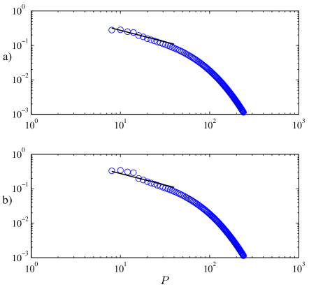
Figure 3: For $K=4$, we plot (a) $\langle\big{|}\partial_{i}u_{j}^{<K}\big{(}|u_{i}^{[\frac{P}{2}-K,P+K]}u_{j}^{[P]}|\big{)}^{<K}\big{|}\rangle/\langle|\Pi_{K}|\rangle$ and (b) $\langle\big{|}\partial_{i}u_{j}^{<K}\big{(}|u_{i}^{[P]}u_{j}^{[\frac{P}{2}-K,P+K]}|\big{)}^{<K}\big{|}\rangle/\langle|\Pi_{K}|\rangle$ using logarithmic bands $[P/2,P]$. The straight lines with $-2/3$ slope are for reference and extend over the fitting region which gives slopes of -0.83 and -0.98 for (a) and (b), respectively. The two plots are essentially identical for large $P$, as expected.

We next present results for the mean quantities $\overline{\Pi}_{K}({\bf u},{\bf u},{\bf u}^{[P]})$ and $\overline{\Pi}_{K}({\bf u},{\bf u}^{[P]},{\bf u}),$ again for $K=4$ and for $P=8-240,$ normalized by the mean flux $\overline{\Pi}_{K}=\varepsilon.$ These data are plotted in Figure 4 and show good agreement with our predictions. When fitted over the “inertial range” from $P=8$ to $P=40$, we obtain a $P^{-1.54}$ scaling for $\overline{\Pi}_{K}({\bf u},{\bf u},{\bf u}^{[P]})$ and $P^{-1.42}$ for $\overline{\Pi}_{K}({\bf u},{\bf u}^{[P]},{\bf u}).$ This is a slightly faster decay than $P^{-4/3}$, again in accord with the recent results by Domaradzki & Carati Domaradzki07b , Domaradzki09 . Note that the plots for $\overline{\Pi}_{K}({\bf u},{\bf u},{\bf u}^{[P]})$ and $\overline{\Pi}_{K}({\bf u},{\bf u}^{[P]},{\bf u})$ are identical for large $P$. This makes good sense, because, as mentioned above, the maximum and middle wavenumbers can differ at most by $K$ and thus those two modes arise from nearly the same wavenumber range. Another interesting feature is that for $P\geq 110$, the partial flux becomes negative. This shows up as a kink on the log-log plot, a feature that was also observed by Domaradzki & Carati Domaradzki09 .

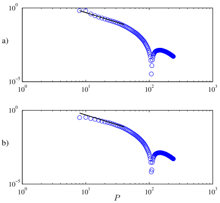
Figure 4: For $K=4$, we plot the global quantities (a) $\overline{\Pi}_{K}({\bf u},{\bf u},{\bf u}^{[P]})/\overline{\Pi}_{K}$ and (b) $\overline{\Pi}_{K}({\bf u},{\bf u}^{[P]},{\bf u})/\overline{\Pi}_{K}$ using logarithmic bands $[\frac{P}{2},P]$. The straight lines with $-4/3$ slope are for reference and extend over the fitting region, which yields slopes of -1.54 and -1.42 for (a) and (b) respectively. The two plots are essentially identical for large $P$. The kink at $P\simeq 110$ in the log-log plot is due to a change in sign at that wavenumber.

C Infrared Locality

We turn now to a discussion of the infrared locality of the spectral energy flux. We shall prove, by similar arguments as in the previous section, that the large-scale components of all three velocity modes—the straining, advecting and advected modes—contribute negligibly to spectral energy flux. The importance of the large-scale advecting mode contribution has, in particular, been a major source of contention in the literature. Several studies BrasseurCorrsin , DomaradzkiRogallo , YeungBrasseur , OhkitaniKida , Alexakisetal05b , DomaradzkiRogallo , OhkitaniKida , Mininni06 employing numerical simulations have concluded that nonlocal advective interactions are primarily responsible for the energy transfer. In this picture, energy cascades to smaller scales by very many small steps in wavenumber, of fixed size, mediated by the largest, energy containing modes. If true, such a picture would have dramatic implications for Kolmogorov’s concept of small-scale universality and on the theory and practice of LES modeling. However, we argue below (and in section III) that this picture is false, and is an artefact of the use of constant (unit) width spectral bands to define energy flux and energy transfer.

1 Theoretical Analysis

We derive exact bounds on the quantities $\Pi_{K}({\bf u}^{[Q]},{\bf u},{\bf u})$, $\Pi_{K}({\bf u},{\bf u}^{[Q]},{\bf u})$, and $\Pi_{K}({\bf u},{\bf u},{\bf u}^{[Q]})$ for $Q\ll K$, thus establishing IR locality in each velocity mode.

We first consider the contribution of the straining mode:

$$\Pi_{K}({\bf u}^{[Q]},{\bf u},{\bf u})=-\partial_{i}u_{j}^{[Q]}\tau_{K}(u_{i},u_{j}).$$ (7)

The origin of IR-locality here is fairly obvious, because the strain from low-wavenumbers is weak. This fact may be expressed as a rigorous upper bound by using the Hölder inequality:

$$\bigg{\langle}\big{|}\partial_{j}u_{i}^{[Q]}\tau_{K}(u_{i},u_{j})\big{|}^{p}\bigg{\rangle}^{1/p}\leq\bigg{\langle}\big{|}{\mbox{\boldmath$\nabla$}}{\bf u}^{[Q]}\big{|}^{r}\bigg{\rangle}^{1/r}\bigg{\langle}\big{|}\tau_{K}({\bf u},{\bf u})\big{|}^{s}\bigg{\rangle}^{1/s}$$

with $\frac{1}{p}=\frac{1}{r}+\frac{1}{s}$. Because $\tau_{K}(u_{i},u_{j})\sim\delta u_{i}(\ell_{K})\delta u_{j}(\ell_{K}),$ it is expected that

$$\bigg{\langle}\big{|}\tau_{K}(u,u)\big{|}^{s}\bigg{\rangle}^{1/s}\sim({\rm const.})u_{rms}^{2}(KL)^{-\rho_{s}}$$ (8)

with $\rho_{s}\doteq 2\sigma_{2s}.$ See Meneveau & O’NeilMeneveauONeil94 and our own figure 6, where we verify this scaling for a sharp spectral filter with $s=2.$ If this result is combined with the scaling relation (4) for the velocity-gradient, we obtain

$$\bigg{\langle}\big{|}\partial_{j}u_{i}^{[Q]}\tau_{K}(u_{i},u_{j})\big{|}^{p}\bigg{\rangle}^{1/p} \leq ({\rm const.})\frac{u_{rms}}{L}(LQ)^{1-\sigma_{r}}~{}u_{rms}^{2}(KL)^{-\rho_{s}}$$ (9)

$$= ({\rm const.})\varepsilon(Q/K)^{1-\sigma_{r}}(KL)^{1-\sigma_{r}-\rho_{s}}.$$ (10)

As long as $\sigma_{r}<1,$ the factor $(Q/K)^{1-\sigma_{r}}$ is decaying for $Q\ll K,$ implying IR locality in the straining mode. Just as in the discussion of UV locality, larger $p$ corresponds to estimates more uniform in space. In the IR case, however, the decay estimates improve for increasing $p$ because $\sigma_{p}$ is non-increasing in $p$ (Frisch Frisch , section 8.4). For example, with $r=s=2p,$ we see that the exponent $1-\sigma_{2p}$ increases with $p$ and the bound on the nonlocal contribution becomes tighter.

Also as in the UV case, there is an additional overall factor $(KL)^{1-\sigma_{r}-\rho_{s}}$ which causes our bound to deteriorate for $KL\gg 1.$ For example, for $p=1,r=s=2,$ $\sigma_{2}+\rho_{2}\doteq\sigma_{2}+2\sigma_{4}$ and the latter is slightly less than $1$ by the concavity of $\zeta_{p}$ as a function of $p.$ (See, for example, Frisch Frisch , section 8.4). However, our bound (10) is still useful (less than $\varepsilon$) if we take $Q$ small enough to offset the slight growth in $K$. Defining the wavenumber $Q_{*}(K)=(1/L)(KL)^{2\sigma_{4}/(1-\sigma_{2})}$ such that $1/L\ll Q_{*}(K)\leq K$, one need only take $Q\ll Q_{*}(K)$ to ensure that the contribution of straining modes at wavenumber $Q$ make a negligible contribution to energy flux.

We now discuss the large-scale contributions of the other two velocity modes which appear through the turbulent stress, i.e. the advecting and advected modes. These two cases are far more delicate. We shall consider in detail the case of the advecting mode, which has been the source of most of the controversy in the literature. Thus, we shall examine

$$\Pi_{K}({\bf u},{\bf u}^{[Q]},{\bf u})=-\partial_{i}u_{j}^{<K}\bigg{[}\big{(}u_{i}^{[Q]}u_{j}\big{)}^{<K}-(u_{i}^{[Q]})^{<K}u_{j}^{<K}\bigg{]}$$ (11)

for $Q<K/2.$ The case of the advected mode is quite similar and will be discussed in parallel. The key to the whole analysis is the following fundamental identity:

$$\Pi_{K}({\bf u},{\bf u}^{[Q]},{\bf u})=-\partial_{i}u_{j}^{<K}\bigg{[}\big{(}u_{i}^{[Q]}u_{j}^{[K-Q,K+Q]}\big{)}^{<K}-u_{i}^{[Q]}u_{j}^{[K-Q,K]}\bigg{]}.$$ (12)

To derive this relation, note that any advected modes $u_{j}$ with wavenumbers $<K-Q$ in (11) when multiplied by $u_{i}^{[Q]}$ will contain only wavenumbers $<K.$ Hence, the low-pass filter $<K$ on the first term in the square bracket $[\cdot]$ can be dropped and the contribution of all such modes cancels exactly with the similar contribution from the second term in the bracket. The additional restriction to wavenumbers $<K+Q$ for $u_{j}$ in the first term arises from the fact that modes with wavenumbers $>K+Q$ when multiplied by $u_{i}^{[Q]}$ can only give wavenumbers $>K$ and these modes do not survive the low-pass filter $<K.$ The identity (12) expresses a basic restriction on the range of interactions allowed to very nonlocal triads, with advecting modes at low wavenumber $Q$ interacting only with advected modes in a band of wavenumbers $[K-Q,K+Q]$ at most, with width $2Q.$ A similar identity can be derived as well for $\Pi_{K}({\bf u},{\bf u},{\bf u}^{[Q]})$, by the same argument. This restriction on the range of the nonlocal triadic interactions is the origin of the IR locality of the SGS spectral flux in the advecting and advected modes.

We now wish to demonstrate this by a rigorous estimate. Unfortunately, the scaling relations (4) that we have employed until now are not applicable to estimate the size of the band-pass field ${\bf u}^{[K-Q,K+Q]}.$ As we mentioned earlier and discuss in more detail in Appendix A, the scaling of $u^{[K]}$ in (4) follows from the empirically-known scaling of velocity-structure functions, but only for $[K]=[K/2,K],$ a logarithmic band. Here, the band $[K-Q,K+Q]$ has a fixed width $2Q$, independent of $K$. However, we may appeal to another empirical observation on the scaling of the turbulent energy spectrum. A great many experiments and simulations have shown that

$$E(k,t)\sim Cu_{rms}^{2}L\,(kL)^{-(1+\zeta_{2})}$$ (13)

with $\zeta_{2}\doteq 2/3,$ for wavenumber binning of unit size. That is, the Kolmogorov power-law spectrum is observed not just with octave bands but with bands of essentially infinitesimal width. This is, in fact, one of the most robust empirical observations on small-scale turbulence. From it we infer that for $Q\ll K$

$$\big{\langle}|{\bf u}^{[K-Q,K+Q]}|^{2}\big{\rangle}=2\int_{K-Q}^{K+Q}dk\,E(k,t)\sim({\rm const.})u_{rms}^{2}(Q/K)(KL)^{-2\sigma_{2}}.$$

The important point here is the factor $(Q/K)$ which becomes smaller with decreasing $Q.$ To exploit this estimate, we use the 4-4-2 Hölder inequality to derive the bound

$$\bigg{\langle}\big{|}\Pi_{K}({\bf u},{\bf u}^{[Q]},{\bf u})\big{|}\bigg{\rangle}\leq({\rm const.})~{}\bigg{\langle}\big{|}{\mbox{\boldmath$\nabla$}}{\bf u}^{<K}\big{|}^{4}\bigg{\rangle}^{\frac{1}{4}}\bigg{\langle}\big{|}{\bf u}^{[Q]}\big{|}^{4}\bigg{\rangle}^{\frac{1}{4}}\bigg{\langle}\big{|}{\bf u}^{[K-Q,K+Q]}\big{|}^{2}\bigg{\rangle}^{\frac{1}{2}}$$

$$\sim({\rm const.})\frac{u_{rms}}{L}(LK)^{1-\sigma_{4}}\cdot u_{rms}(LQ)^{-\sigma_{4}}\cdot u_{rms}(Q/K)^{1/2}(KL)^{-\sigma_{2}}$$

$$\sim({\rm const.})\varepsilon(LK)^{1-\sigma_{2}-2\sigma_{4}}(Q/K)^{1/2-\sigma_{4}}.\,\,\,\,\,\,\,\,\,\,\,\,\,\,\,\,\,\,\,\,\,\,\,\,\,\,\,\,\,\,\,\,\,\,\,\,\,\,\,\,\,\,\,\,\,\,\,\,\,\,\,$$ (14)

See Appendix A for more details. Since $\sigma_{4}$ is known empirically to be a bit smaller than $1/3,$ the exponent $1/2-\sigma_{4}>1/6$ and thus the factor $(Q/K)^{1/2-\sigma_{4}}$ becomes small for $Q\ll K.$ This proves the IR locality in the advecting mode of spectral SGS flux. The result is due to two competing factors. On the one hand, the low-wavenumber velocity modes have greater magnitude, reflected in the factor $u_{rms}(LQ)^{-\sigma_{4}}$ which grows for decreasing $Q.$ On the other hand, the modes with low wavenumber $Q$ are restricted to interact with a smaller set of modes at wavenumber $K,$ reflected in the decreasing factor $(Q/K)^{1/2}$. The latter factor wins the competition, implying IR locality. This is one of the most important results established in our paper.

As with our earlier bounds, there is a troublesome factor $(LK)^{1-\sigma_{2}-2\sigma_{4}}$ that grows with $K.$ However, defining $Q_{*}(K)\equiv K(KL)^{2\sigma_{2}/(1-2\sigma_{4})-2}$ so that $1/L\ll Q_{*}(K)\leq K,$ we see that our bound becomes $\ll\varepsilon$ for $Q\ll Q_{*}(K).$ Thus, IR locality follows, although the result is presumably not optimal. EyinkEyink05 (and I) used graded filters to derived a sharper bound of the form $O((Q/K)^{2/3}),$ whereas the decay proved here for the sharp spectral filter is only like $(Q/K)^{1/6}.$ As we shall discuss below, there is some evidence from our numerics to suggest that the 2/3 decay rate holds also for absolute spectral flux and even faster decay is expected for mean spectral flux due to decorrelation effects.

First, however, let us discuss briefly how the bound (14) is reconciled with the 1994 counterexample of EyinkEyink94 which showed that spectral flux may be dominated by nonlocal advective sweeping interactions. The counterexample cannot satisfy the bound (14), which would imply instead that the local triads dominate. There is no contradiction, however. Eyink’s counterexample is a Fourier-Weierstrass-type function given by a lacunary Fourier series, with just two wavenumber modes in each octave band $[2^{N},2^{N+1}]$ for $N=1,2,3,...$. It has scaling properties similar to those of a turbulent velocity field (like (4)), but it fails to satisfy the strong condition (13) on the energy spectrum because its wavenumber modes do not densely populate Fourier space. In this respect, the counterexample appears very different from typical turbulent velocity fields. Thus, it is true as a general mathematical fact that energy flux defined by the sharp spectral filter may be dominated by nonlocal triads (unlike flux defined with graded filters). However, this is not the case for the turbulent fields satisfying condition (13). In particular, the counterexample of Eyink is only slightly related to the “local transfer by nonlocal triads” observed in turbulent simulationsBrasseurCorrsin , DomaradzkiRogallo , YeungBrasseur , OhkitaniKida , Alexakisetal05b , DomaradzkiRogallo , OhkitaniKida , Mininni06 . As we shall discuss in section III, those DNS observations are completely compatible with locality of energy cascade.

All of our results on IR locality have, to this point, been mathematically rigorous upper bounds. However, we expect much faster decay of non-local contributions for the space-average flux than the bounds proved above, due to cancellation of fluctuating positive and negative parts. It is possible to provide more physical arguments to explain what we believe is the true scaling of IR non-local contributions to mean spectral flux. For details, see I and AluieThesis . Here we note just the final results that

$$\overline{\Pi}_{K}({\bf u}^{[Q]},{\bf u},{\bf u}),\,\,\,\,\overline{\Pi}_{K}({\bf u},{\bf u}^{[Q]},{\bf u})\sim\varepsilon\bigg{(}\frac{\ell_{K}}{\ell_{Q}}\bigg{)}^{1+\zeta_{1}}.$$ (15)

The result is different for locality in the advected mode, so we give a few details. By wavenumber conservation with $Q<K$:

$$\overline{\Pi}_{K}({\bf u},{\bf u},{\bf u}^{[Q]})=\langle\partial_{i}u_{j}^{[Q]}u_{i}^{>K}u_{j}^{[K-Q,K]}\rangle=\langle\partial_{i}u_{j}^{[Q]}u_{i}^{>K}u_{j}^{>K-Q}\rangle-\langle\partial_{i}u_{j}^{[Q]}u_{i}^{>K}u_{j}^{>K}\rangle.$$

The limited number of modes contributing to $u_{j}^{[K-Q,K]}$ leads to a major cancellation. Indeed, expressing the triple correlation heuristically as increments and using fusion rules as in I, we obtain the scaling result for $Q\ll K$

$$\overline{\Pi}_{K}({\bf u},{\bf u},{\bf u}^{[Q]}) \sim u^{3}_{rms}\frac{\ell_{K}}{\ell^{2}_{Q}}\bigg{(}\frac{\ell_{Q}}{L}\bigg{)}^{\zeta_{3}}\Big{[}\bigg{(}\frac{\ell_{K-Q}}{\ell_{Q}}\bigg{)}^{\zeta_{1}}-\bigg{(}\frac{\ell_{K}}{\ell_{Q}}\bigg{)}^{\zeta_{1}}\Big{]}$$

$$\sim \varepsilon\frac{\ell_{K}}{\ell_{Q}}\Big{[}\frac{\ell_{K}}{\ell_{Q}}\cdot\bigg{(}\frac{\ell_{K}}{\ell_{Q}}\bigg{)}^{\zeta_{1}}\Big{]}=\varepsilon\bigg{(}\frac{\ell_{K}}{\ell_{Q}}\bigg{)}^{2+\zeta_{1}}.$$

The cancellation leads to an additional factor of $\ell_{K}/\ell_{Q},$ which gives a faster decay for this non-local contribution.

It is worth noting that a similar cancellation appears in the partial flux $\overline{\Pi}_{K}({\bf u},{\bf u}^{[Q]},{\bf u}),$ where it is crucial to give the scaling $\sim(\ell_{K}/\ell_{Q})^{1+\zeta_{1}}$ in (15). The physics behind IR locality in the advecting mode is that when $Q$ is very small, then, due to wavenumber conservation, only a few wavenumber modes within distance $Q$ of $K$ contribute to the flux, implying insignificant transfer from those triads. In section III we shall rederive this result within the ALHDIA closure of KraichnanKraichnan66 , which embodies in a quantitative form the same basic ideas employed heuristically above. As for the UV case, our prediction of the IR non-locality correction scaling as $(Q/K)^{1+\zeta_{1}}$ can in principle be distinguished from the scaling prediction $(Q/K)^{2-\zeta_{2}}$ of KraichnanKraichnan66 and L’vov & FalkovichLvovFalkovich , due to small effects of intermittency.

2 Numerical Results

We now present simulation results on IR locality. We first consider space-averages of the absolute values of the partial fluxes. These should be devoid of any cancellation effects but are constrained by our rigorous upper bounds. In Fig.5 we plot $\langle\big{|}\Pi_{K}({\bf u}^{[Q]},{\bf u},{\bf u})\big{|}\rangle$ ($\circ$), $\langle|\Pi_{K}({\bf u},{\bf u},{\bf u}^{[Q]})|\rangle$ ($\times$) and $\langle|\Pi_{K}({\bf u},{\bf u}^{[Q]},{\bf u})|\rangle$ ($+$), for $K=100$ and for $Q$ ranging continuously over all wavenumbers $Q\leq K/2$. Fitting with power-laws over the “inertial-range” from $Q=8$ to $Q=40$ gives scalings of $Q^{0.77}$, $Q^{0.42}$ and $Q^{0.45},$ respectively. The first is in good agreement with our rigorous estimate $(Q/K)^{1-\sigma_{2}},$ for $\sigma_{2}\doteq 1/3$. The other two quantities have scaling exponents exactly between the value $2/3$ and the $1/6$ exponent of our rigorous upper bound. In Fig.6 we also test the scaling prediction (8) of the spectral SGS stress for $s=2$ and obtain good agreement with the K41 value exponent $\rho_{2}\doteq 2\sigma_{4}\doteq 2/3.$

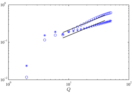
Figure 5: For $K=100$, we plot $\langle|\Pi_{K}({\bf u}^{[Q]},{\bf u},{\bf u})|\rangle/\langle|\Pi_{K}|\rangle$ ($\circ$); $\langle|\Pi_{K}({\bf u},{\bf u},{\bf u}^{[Q]})|\rangle/\langle|\Pi_{K}|\rangle$ ($\times$); and $\langle|\Pi_{K}({\bf u},{\bf u}^{[Q]},{\bf u})|\rangle/\langle|\Pi_{K}|\rangle$ ($+$) using logarithmic bands $[Q/2,Q]$. The straight lines are for reference and have a $2/3$ slope. They extend over the fitting region which yields slopes of 0.77, 0.42, and 0.45 for ($\circ$), ($\times$), and ($+$), respectively. Plots ($\times$) and ($+$) are almost identical, as expected.

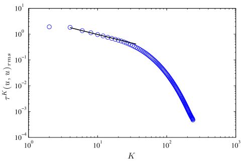
Figure 6: The $rms$ stress $\big{(}{\mbox{\boldmath$\tau$}}_{K}({\bf u},{\bf u})\big{)}_{rms}/E_{total}$ normalized by the energy of the system and plotted as a function of $K$. The straight line with -2/3 slope is for reference and extends over the fitting region which gives a slope of -0.71.

In Fig. 7 we plot $-\langle\Pi_{K}({\bf u}^{[Q]},{\bf u},{\bf u})\rangle$ ($\circ$), $\langle\Pi_{K}({\bf u},{\bf u},{\bf u}^{[Q]})\rangle$ ($\times$), and $\langle\Pi_{K}({\bf u},{\bf u}^{[Q]},{\bf u})\rangle$ ($+$). Fitting with a power-law over the range $Q=8$ to $Q=40$, we obtain scaling laws of $Q^{1.08}$, $Q^{1.90},$ and $Q^{1.27},$ respectively, in fairly good agreement with our heuristic estimates $Q^{4/3},Q^{7/3}$ and $Q^{4/3}.$ The IR decay rates are a little slower than those predicted, in agreement with the findings of Domaradzki & CaratiDomaradzki07b , Domaradzki09 . This can be attributed to the extreme shortness of the inertial range and the relatively smooth velocities at large scales in the simulation. Note that $\langle\Pi_{K}({\bf u}^{[Q]},{\bf u},{\bf u})\rangle<0$ over the range of the graph, becoming positive for $Q>60$. This can be understood in terms of detailed balance of energy in which the band of wavenumber modes $[Q]$ is receiving energy from modes $>K$, but the amount getting progressively smaller for $Q\ll K$ and more negligible compared to the positive total mean flux $\langle\Pi_{K}\rangle$.

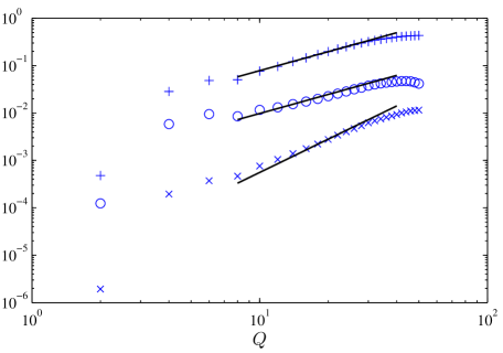
Figure 7: For $K=100$, we plot $-\langle\Pi_{K}({\bf u}^{[Q]},{\bf u},{\bf u})\rangle/\langle\Pi_{K}\rangle$ ($\circ$); $\langle\Pi_{K}({\bf u},{\bf u},{\bf u}^{[Q]})\rangle/\langle\Pi_{K}\rangle$ ($\times$); and $\langle\Pi_{K}({\bf u},{\bf u}^{[Q]},{\bf u})\rangle/\langle\Pi_{K}\rangle$ ($+$) using logarithmic bands $[Q/2,Q]$. The straight lines are for reference and have $4/3$ and $7/3$ slopes. They extend over the fitting region which gives slopes of 1.08, 1.90, and 1.27 for ($\circ$), ($\times$), and ($+$) respectively.

III Comparison with Previous Work

Our entire analysis of the preceding section considered the SGS spectral energy flux (3). It is more traditional to base discussions of wavenumber locality in turbulence on the triplet transfer function

$$\overline{T}({\bf k},{\bf q},{\bf p})={\rm Re}\,\{ik_{i}\langle\widehat{u}^{*}_{j}({\bf k})\widehat{u}_{i}({\bf q})\widehat{u}_{j}({\bf p})\rangle\}\delta_{{\bf k},{\bf p}+{\bf q}}.$$

This function can be interpreted as giving the mean rate of energy transfer into wavenumber mode ${\bf k}$ from mode ${\bf p}$ induced by mode ${\bf q}$ and satisfies the “detailed conservation” propertyOnsager49 :

$$\overline{T}({\bf k},{\bf q},{\bf p})+\overline{T}({\bf k},-{\bf q},{\bf p})=0.$$

This transfer function is often integrated over spherical shells to define a quantity $\overline{T}(k,q,p)$ which depends only upon wavenumber magnitudes $k,p,q,$ restricted to values which can be assumed by the side-lengths of a closed triangle. In numerical simulations DomaradzkiRogallo , OhkitaniKida , Alexakisetal05b , Mininni06 this quantity is represented by

$$T(K,Q,P)=\partial_{i}u^{[K-1,K]}_{j}u^{[Q-1,Q]}_{i}u^{[P-1,P]}_{j},$$ (16)

using band-pass velocity fields ${\bf u}^{[K-1,K]}$ with bands of unit width. This function is defined pointwise in space, although usually its spatial average is taken over the flow domain.

From the triplet transfer $\overline{T}(k,q,p)$ one can obtain the mean spectral flux as

$$\overline{\Pi}_{K}=-\int_{0}^{K}dk\int_{0}^{\infty}dq\int_{0}^{\infty}dp\,\,\overline{T}(k,q,p),$$ (17)

or, pointwise in space,

$$\Pi_{K}^{uns}=-\sum_{K^{\prime}<K,Q^{\prime},P^{\prime}}T(K^{\prime},Q^{\prime},P^{\prime})=-\partial_{i}u^{<K}_{j}(u_{i}u_{j}).$$ (18)

As discussed earlier, this quantity has the same space-average value as the SGS energy flux (3). However, its pointwise properties are quite different, since it is not Galilei-invariant unless averaged over space. Thus, the conventional spectral flux (18), and also its variant form $-\partial_{i}u^{<K}_{j}(u_{i}u_{j})^{<K}$, are pointwise scale-nonlocal objects, dominated by large-scale advection effects. All such sweeping interactions, however, can be associated to space-transport of energy, with the SGS energy flux remaining as the unique pointwise Galilei-invariant measure of energy transfer to small-scales. See EyinkEyink95 , Eyink05 and I. It was for this reason that we chose to analyze the spectral SGS flux in the previous section, since it enjoys much better scale-locality properties than the conventional spectral flux.

On the other hand, the conventional spectral flux when averaged over space (or, assuming ergodicity, over time or over ensembles) is also dominated by local triadic interactions. This was realized by the early pioneers of the subjectObukhov41a , Obukhov41b , Onsager45 , Onsager49 , Heisenberg48 and analyzed in detail by KraichnanKraichnan59 , Kraichnan66 , Kraichnan71 using closure approximations. A careful examination of Kraichnan’s works shows that his arguments for scale-locality are based on the same basic ingredients as our rigorous proofs in the previous section. We shall briefly review here the asymptotic analysis in section 3 of Kraichnan (1966)Kraichnan66 using the ALHDIA closure, in order to discuss its relation to our arguments and also to facilitate later comparison with the numerical studies BrasseurCorrsin , DomaradzkiRogallo , YeungBrasseur , OhkitaniKida , Alexakisetal05b , Mininni06 , Mininni08 , Domaradzki07a , Domaradzki07b , Domaradzki09 . In order to make direct contact between our proof and Kraichnan’s analysis it is convenient to consider the quantity

$$\overline{\Pi}_{K}({\bf u},{\bf u}^{[Q]},{\bf u})=-\int_{0}^{K}dk\int_{Q/2}^{Q}dq\int_{K}^{\infty}dp\,\,\overline{T}(k,q,p),$$ (19)

which measures the mean energy flux due to advection by modes in the wavenumber band $[Q].$ KraichnanKraichnan66 considered a slightly different set of quantities—in his notations, $T_{<Q}(K)$ and $\Pi_{<Q}(K)$— or the transfer and flux due to advection by all modes with wavenumbers $<Q.$ He obtained asymptotic expressions for these in the limit $Q\ll K.$ However, his analysis and results carry over essentially to the flux quantity (19).

An important fact used by Kraichnan in his analysis is that, due to wavenumber conservation, this partial flux may be written as

$$\overline{\Pi}_{K}({\bf u},{\bf u}^{[Q]},{\bf u})=-\int_{Q/2}^{Q}dq\int_{K-q}^{K}dk\int_{K}^{k+q}dp\,\,\overline{T}(k,q,p).$$ (20)

Introducing dimensionless variables $u,v$ by $k=K-qv,\,p=K+qu,$ this may be rewritten as

$$\overline{\Pi}_{K}({\bf u},{\bf u}^{[Q]},{\bf u})=-\int_{Q/2}^{Q}dq\,q^{2}\int_{0}^{1}dv\int_{0}^{1-v}du\,\,\overline{T}(K-qv,q,K+qu).$$ (21)

The result (21) is exact, involving no approximation. It shows that the restriction on allowed wavenumbers interactions provides an additional small factor of $q^{2}$ for small $q,$ which proves essential to obtain IR spectral locality.

To proceed further requires an explicit expression for the transfer function. Kraichnan’s ALHDIA closure yields the formula

$$\overline{T}(k,q,p,t)\equiv\hat{B}_{kpq}\Delta_{kpq}\int_{t_{0}}^{t}ds\big{[}G(k;t|s)U(p;t|s)-G(p;t|s)U(k;t|s)\big{]}U(q;t|s);$$ (22)

see equation (2.6) of Kraichnan (1966)Kraichnan66 . Here $U(k;t|s)$ and $G(k;t|s)$ are 2-time Lagrangian velocity-correlation and mean-response functions. The factor $\Delta_{kpq}$ is equal to 1 if the wavenumbers $k,p,q$ can be the sides of a closed triangle and is equal to 0 otherwise. Finally, the factor $\hat{B}_{kpq}=4\pi^{2}k^{2}p^{2}q(xy+z^{3}),$ where $x=\cos\alpha,y=\cos\beta,z=\cos\gamma$ are the cosines of the angles $\alpha,\beta,\gamma$ that are opposite to sides of length $k,p,q$ in the wavenumber triangle. Substituting the steady-state, inertial-range scaling forms

$$G(k;t|s)=g(\varepsilon^{1/3}k^{2/3}(t-s)),\,\,\,\,U(k;t|s)=\frac{C}{2\pi}\varepsilon^{2/3}k^{-11/3}r(\varepsilon^{1/3}k^{2/3}(t-s)),$$ (23)

one obtains the asymptotic expression for $k=K-qv,\,p=K+qu,$ and $q\ll K$

$$\overline{T}(k,q,p)\simeq-\varepsilon w(1-w^{2})C^{2}IK^{-4/3}q^{-5/3},$$ (24)

where $w=u+v$ and $I$ is an integral over the scaling functions $g(\tau),r(\tau).$ See KraichnanKraichnan66 and Appendix B for details. We just note here one signficant feature of the calculation, which is the near cancellation between the two input and output terms in (22) for $k\approx p\approx K.$ The physics of this was discussed by KraichnanKraichnan66 , p.1733:

“These terms separately give contributions proportional to the energy in the wavenumbers $<q,$ not to the mean-square vorticity. …The input and output contributions from low wavenumbers are proportional to energy because they represent convection as well as straining. Convection of high-wavenumber structures by strongly excited low-wavenumber velocity components implies a rapid exchange of phase of the high-wavenumber Fourier amplitudes…. This exchange is represented in (2.6) [our (22)] by the large, cancelling input and output contributions. The net contribution $T_{<q}(k,t)$ represents the effect of straining alone.”

These remarks are consistent with our observation that the spectral energy flux $\Pi_{K}^{uns}$ in (18) is pointwise non-local and dominated by convective sweeping, with such effects only cancelling in the average over space. The cancellation between input and output terms for $k\approx p\approx K$ also yields an additional small factor of $q$ crucial to the final result.

Substituting the closure approximation (24) into the expression (21) yields finally that

$$\overline{\Pi}_{K}({\bf u},{\bf u}^{[Q]},{\bf u})\simeq{\mathcal{C}}\varepsilon\left(\frac{Q}{K}\right)^{4/3},\,\,\,\,\,\,\,\,\,Q\ll K,$$ (25)

for ${\mathcal{C}}=\frac{1}{10}C^{2}I\big{(}1-\frac{1}{2^{4/3}}\big{)}\doteq 0.503.$ For details, see Appendix B. We thus recover Kraichnan’s 4/3 scaling law for decay of IR-nonlocal contributions. The factor $Q^{4/3}$ arises from integration of the product $q^{1/3}=q^{2}q^{-5/3}$ over the octave band $[Q/2,Q].$ Just as in our rigorous proof in the preceding section, there is a competition between the decaying factor $q^{2}$ which arises from the restriction on wavenumber interactions and the growing factor $q^{-5/3}$ which arises from the increase in energy of low-wavenumber modes. For a similar calculation and analysis, see Verma et al.Vermaetal , section 3.

We have focused so far on energy flux but many studies DomaradzkiRogallo , OhkitaniKida , Alexakisetal05b , Mininni06 , Mininni08 , Domaradzki07a , Domaradzki07b , Domaradzki09 instead consider energy transfer between wavenumber bands. Our results also imply scale-locality of suitable transfers. Note, for example, that the partial flux in (20) for $Q<K/2$ equals

$$\overline{\Pi}_{K}({\bf u},{\bf u}^{[Q]},{\bf u}) = \overline{\Pi}_{K}({\bf u}^{[K]},{\bf u}^{[Q]},{\bf u}^{[P]})$$ (26)

$$= -\int_{K/2}^{K}dk\int_{Q/2}^{Q}dq\int_{P/2}^{P}dp\,\,\overline{T}(k,q,p),$$ (27)

$$\equiv -\overline{T}([K],[Q],[P]),$$ (28)

with $P=2K.$ In the last line we have defined the mean triplet transfer function with octave bands $[K]=[K/2,K].$ Because this quantity equals the partial flux, our previous bounds and scaling results all apply, showing that this quantity for $Q\ll K$ is negligible compared with the total transfer rate from adjacent band interactions.

It is very important for the closure calculation presented in this section and also for the rigorous proof in the preceding section that such logarithmic bands be employed. When demonstrating IR locality in the advecting mode, we have used the fact that modes with wavenumbers $Q\ll K$ interact with a very restricted subset of the modes contained in ${\bf u}^{[P]}$, resulting in an overall weak contribution to the flux. On the other hand, if linear bands are used, the modes contributing to ${\bf u}^{[P-1,P]}$ are already restricted and, thus, taking $Q$ smaller does not impose any further restriction. Thus, the space-average of $T(K,Q,P)$ in (16) must increase for smaller $Q$ simply because ${\bf u}^{[Q]}$ gets bigger at the larger scales, where most of the energy resides. This can be verified directly from the asymptotic formula (24) of the ALHDIA closure for $\overline{T}(k,q,p),$ which is essentially the same quantity. However, $T(K,Q,P)$ and other such objects which compare single triads vastly underestimate the contribution from the local triads, which, when taken into account cumulatively, swamp the non-local interactions through sheer number.

Such remarks apply to studies which have claimed to verify a cascade mechanism of “local transfer by nonlocal triads” in numerical simulations. For example, several such worksDomaradzkiRogallo , OhkitaniKida , Alexakisetal05b , Mininni06 have calculated the partially-summed transfer

$$\overline{T}(K,P)=\sum_{Q}\overline{T}(K,Q,P)=\frac{1}{V}\int d^{3}x\,\,\partial_{i}u_{j}^{[K-1,K]}u_{i}u_{j}^{[P-1,P]}.$$

This can be interpreted as the mean rate of energy transfer into wavenumber band $[K-1,K]$ from band $[P-1,P],$ mediated by all other wavenumbers. The cited numerical studies have found that the energy transfer to the $K$th band has largest positive contribution from $P=K-k_{f}$ and largest negative contribution from $P=K+k_{f}$, mediated by modes at the forcing wavenumber $k_{f}$. This result was suggested to support the dominance of nonlocal triads in energy cascadeDomaradzkiRogallo , OhkitaniKida , Alexakisetal05b , Mininni06 . In fact, the result should have been expected and is completely consistent with scale-local interactions! Notice that this behavior is predicted, for example, by the asymptotic formula (24) from Kraichnan’s ALHDIA closure, since its integral over $q$ is clearly dominated by the peak of the $q^{-5/3}$ spectrum at $q=k_{f}.$ However, Kraichnan correctly deduced from this expression that cascade proceeds by the local triads, not the non-local triads. This can be seen by considering instead the similar quantity

$$\overline{T}([K],[P])=\frac{1}{V}\int d^{3}x\,\,\partial_{i}u_{j}^{[K]}u_{i}u_{j}^{[P]},$$

employing octave bands. Our previous discussion applies to this object, showing that the non-local triads make a negligible contribution.

To underline this conclusion, we shall exhibit illustrative numerical results from a $512^{3}$ simulation using hyperviscosity BorueOrszag95 :

$$\partial_{t}{\bf u}+({\bf u}\cdot{\mbox{\boldmath$\nabla$}}){\bf u}=-{\mbox{\boldmath$\nabla$}}p+\nu_{10}({\mbox{\boldmath$\nabla$}}^{2})^{5}{\bf u}+{\bf f}$$ (29)

We employed the same forcing (2) as for our viscous simulations but with $k_{f}=1,$ and we took hyperviscous coefficient $\nu_{10}=2\times 10^{-21}$. These choices were made to achieve a constant mean energy flux $\overline{\Pi}_{K}=\varepsilon$ over as long a range of wavenumbers as possible. See Figure 8a. Just below, in Figure 8b, we plot $\overline{T}(K,P)$ for linear bins magnified by a factor of 10 (dashed line) and $\overline{T}([K],[P])$ for octave bands (solid line). Both quantities are plotted as functions of $P$ for $K=50$ and have been normalized by the mean flux $\varepsilon.$

The results for unit-width bands agree with those of the earlier studiesDomaradzkiRogallo , OhkitaniKida , Alexakisetal05b , Mininni06 , while those for octave bands are similar to those presented by Verma et al. Vermaetal , Figure 5 for logarithmic bands (base-$\sqrt{2}$ rather than our base-$2$). However, it is quite instructive to plot the two quantities together. The result for $\overline{T}(K,P)$ illustrates the contribution of “local transfer by nonlocal triads”, with the familiar feature of peaks separated by $2k_{f}.$ Notice, however, that the magnitude is miniscule compared both with the mean flux $\varepsilon$ and also with the summed effect of all the local triads, which dominates in $\overline{T}([K],[P]).$ This kind of transfer will become an even smaller fraction of the total for larger $K,$ decreasing as $\sim K^{-4/3}$ according to the Kraichnan estimate (25). The plot of $\overline{T}([K],[P])$ shows that transfer into $[K]$ has largest positive contribution from the octave band $[P]$ with $P\approx K/2$ and largest negative contribution from the band with $P\approx 2K.$ This demonstrates the multiplicative, self-similar nature of the local cascade.

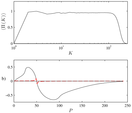
Figure 8: Using data from the hyperviscous simulation, we plot (a) the energy flux $\langle\Pi_{K}\rangle$. In (b), we plot, for $K=50$, as a function of $P$: (solid) $\langle\partial_{i}u_{j}^{[K]}u_{i}u_{j}^{[P]}\rangle/\langle\Pi_{K}\rangle$ using octave bands $[K/2,K],\,[P/2,P]$, and (dashed) $10\times\langle\partial_{i}u_{j}^{[K-1,K]}u_{i}u_{j}^{[P-1,P]}\rangle/\langle\Pi_{K}\rangle$ using linear bands. We multiply the latter by $10$ for comparison. The dashed-line plot shows energy transfer in incremental steps with the distance between peaks being $2$, which is twice the forcing wavenumber, $k_{f}=1$.This kind of transfer represents a negligible fraction of the flux $\langle\Pi_{K}\rangle$, as the plot shows, which will decrease even more ($\sim K^{-4/3}$) for larger $K$. The solid-line plot has peaks at $P=32$ and $88$, showing transfer in multiplicative steps. The solid-line decays like $P^{1.12}$ over the range $[1,30]$, quite close to the expected power $P^{4/3}$. There is no similar discernible power-law decay in the ultraviolet limit of large $P$ due to dissipation.

Our results rigorously disprove a number of suggestions in the recent literature. Alexakis et al. (2005)Alexakisetal05b and Mininni et al. (2006,2008)Mininni06 , Mininni08 have claimed on the basis of $1024^{3}$ and $2048^{3}$ DNS that the ratio $\overline{\Pi}_{K}({\bf u},{\bf u}^{[Q]},{\bf u})/\overline{\Pi}_{K}$ with $Q\simeq k_{F}$ asymptotes to a value of about $0.10$-$0.20$ for large $K$ in the inertial range. A long plateau within the inertial range is ruled out by our rigorous estimate (14) which shows that this quantity is bounded at least as $O(\varepsilon(KL)^{-\alpha})$ for large $K,$ with $\alpha=\sigma_{2}+\sigma_{4}-1/2\doteq 1/6.$ According to the estimate (25) from Kraichnan’s ALHDIA closure theory, the decay rate is actually $\sim\varepsilon(KL)^{-4/3},$ which is even faster. Whatever is the explanation of the plateau observed in the reported simulations Alexakisetal05b , Mininni06 , Mininni08 it cannot be an inertial range effect. Indeed, the asymptote observed in their numerical data occurs at high wavenumbers $K$ beyond the constant flux inertial range and within the pronounced “bottleneck” of their energy spectrum. A Reynolds-number dependence of the plateau level has furthermore been reported in the most recent paperMininni08 (see Fig.4 there)

$$\frac{\overline{\Pi}_{K_{\lambda}}({\bf u},{\bf u}^{[k_{F}]},{\bf u})}{\overline{\Pi}_{K_{\lambda}}}\sim Re^{-\beta},\,\,\,\,\,\mbox{$\beta\doteq$ 0.6\textendash 0.7},$$

where $K_{\lambda}$ is the Taylor-scale wavenumber. Since $L/\lambda\simeq Re^{1/2},$ this is completely consistent with Kraichnan’s estimate (25), which would yield a scaling law $Re^{-2/3}$ for the above ratio. Inertial-range theory cannot explain, however, why the fraction stays constant for $K>K_{\lambda}.$ We conjecture that this is an effect of the bottleneck. In Figure 9 we plot the same ratio using data from our hyperviscous simulation. It shows a decay very close to $K^{-4/3}$ through the inertial range, until it asymptotes at $2$-$3\%$ over the region of the bottleneck, which is known to be more prominent for hyperviscosity Biskampetal98 , HaugenBrandenburg . Note that we do not observe a similar plateau in our simulation with regular viscosity, which does not have a conspicuous bottleneck (see Fig.1).

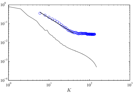
Figure 9: Using data from the hyperviscous simulation, we plot $\langle\Pi_{K}({\bf u},{\bf u}^{<6},{\bf u})\rangle/\langle\Pi_{K}\rangle$ ($\circ$) as a function of $K$. The straight line with slope $-4/3$ is for reference and extends over the fitting range of the graph, which gives a decay rate of $K^{-1.32}$. Beyond this range, the plot asymptotes at $2$-$3\%$. The plot of the energy spectrum (solid line) suggests that this trend is related to the bottleneck in the crossover between the inertial and dissipation ranges of the spectrum.

Alexakis et al. (2005)Alexakisetal05b and Mininni et al. (2006,2008) Mininni06 , Mininni08 have further speculated that their numerical results—which they interpreted to show the dominance of non-local interactions to mean transfer—may be due to intermittency and long-lived vortical structures. However, the bounds on space-average energy flux in the current work are little affected by intermittency, since they involve only low-order scaling exponents $\sigma_{p}$ with $p=2\sim 4.$ Our estimates for large $p$ and the pointwise estimates for graded filtersEyink05 , EyinkAluie will indeed be modified by intermittency, which has the effect of improving the IR estimates and degrading the UV estimates. UV locality will nevertheless hold at every space point with a positive Hölder exponent of the velocity field.

IV Conclusions

We have proved by rigorous estimates that spectral energy flux in three-dimensional turbulence is dominated by local wavenumber triads. No additional averaging over scales, as in Eyink (1994)Eyink94 , was required. Furthermore, we showed that spectral locality holds without additional cancellations resulting from space averaging, which, when included, further decrease the net non-local contribution. Our proof exploited four main ingredients: (1) The SGS spectral energy flux, which is the unique Galilei-invariant measure of the energy flux across scales. It has the sweeping effects subtracted, which is essential to prove infrared locality. (2) Scaling properties that are observed empirically to hold for the turbulent velocity field. In particular, we employ the strong scaling condition eq.(13) on the energy spectrum, which rules out the mathematical counterexample of EyinkEyink94 . (3) Wavenumber conservation, which restricts the range of interactions in Fourier space. (4) Logarithmic bands of wavenumber modes which, unlike linear bands, represent the cumulative effect of the growing number of local triads.

We were thus able to explain the results of previous research claiming the dominance of non-local interactions in the energy cascade DomaradzkiRogallo , OhkitaniKida , Alexakisetal05b , Mininni06 . Since these studies used linear bands in decomposing the velocity field, they were effectively comparing triads of single Fourier modes with each other. The most dominant of these triads are the ones with a large-scale advecting mode. However, such non-local triads are few, an idea implicit in the work of Kraichnan (1966)Kraichnan66 and emphasized more recently by Verma et al. (2005) Vermaetal . Thus, their effect becomes more negligible as the energy cascades to smaller scales, whereas the number of local triads grows geometrically, swamping the non-local effects. Therefore, the Kolmogorov picture of local cascade is consistent with the presence of non-local triadic interactions, since these become vanishingly insignificant in a longer inertial-range.

We find that the scale-locality properties of the SGS flux with a sharp spectral filter are close to those with graded filters established by EyinkEyink95 , Eyink05 and in paper I. Our numerical results for the space-average of the SGS spectral flux are essentially the same as those for graded filters, in agreement with the earlier findings of Domaradzki & CaratiDomaradzki07a , Domaradzki07b . The locality properties of the SGS spectral flux $\Pi_{K}$ are possibly not quite as good pointwise as those of SGS flux with graded filters. We could prove some nearly uniform estimates on UV and IR locality, but with decay rates that are probably sub-optimal and with additional $K$-dependent factors. More seriously, we could not prove pointwise estimates on the SGS spectral flux involving the local Hölder exponent at the space point ${\bf x}$. However, we would like to moderate the claim of EyinkEyink05 that spectral energy flux “is an inappropriate measure of energy transfer.” This is true for the unsubtracted flux $\Pi_{K}^{uns},$ which is pointwise non-Galilei-invariant and becomes scale-local only when averaged over space. On the other hand, the SGS spectral flux $\Pi_{K}$ is scale-local, even in the absolute sense, without cancellations due to space-averaging. In particular, the sharp spectral filter has a sound theoretical basis for use in large-eddy simulation (LES) modeling of turbulent energy cascade.

The width of wavenumber bands is more important for scale-locality than the grading of the filter kernel. As we have seen, transfer functions for individual wavenumber triads or transfer functions with wavenumber bands of fixed width on a linear scale may have the greatest magnitude for non-local triads. The situation is completely different for transfer functions with bands of fixed width on a logarithmic scale. The transfers for such logarithmic bands are dominated by local triad interactions, which, by their vastly greater numbers, overwhelm the contribution of the non-local triads. Only the collective contribution of the local triads is large enough to explain the observed flux of energy to small scales. In addition, it is only quantities summed over logarithmic bands which can be simultaneously localized both in scale and in space. This is a basic fact of harmonic analysis, equivalent to the Heisenberg uncertainty principleJaffardetal01 . To constitute an “eddy” of half the size requires twice as many wavenumber modes to achieve the necessary localization in space. If one believes, as we do, that the essential dynamics of turbulent cascade involves modes resolved both in scale and in space, then summation over logarithmic wavenumber bands is necessary to its physical description.

Fourier series, without a doubt, are often a useful tool to analyze turbulent cascades. However, individual Fourier modes have no physical significance and it is dangerous to think of the elementary interactions as those involving individual wavenumber triads. A single Fourier mode is a wave which extends periodically throughout all space, whereas incompressible fluids (when constant-density, non-rotating, etc.) exhibit no linear wave phenomena. Consider the case of turbulent flow in a wall-bounded domain, like air in a room or water in a cup. The velocity field for such a flow may be decomposed into Fourier modes by imbedding the flow domain in a periodic box. A single triad then represents interacting periodic waves, exchanging energy beyond the solid walls of the domain! This clearly has no physical reality. Fourier modes are only one convenient basis, among many, that may be used in the scale decomposition of the velocity field, and the physics cannot depend on the expansion coefficients of any particular basis. Only the sum over the basis elements can have intrinsic meaning.

We have proved in this work that, asymptotically for long inertial ranges, the energy cascade proceeds neither in large strides between widely separated Fourier bands nor in small incremental wavenumber steps. Rather, it proceeds in multiplicative steps between Fourier bands which are adjacent to each other on a logarithmic scale. However, the bounds on the non-local triad contributions to energy flux decay only as power-laws, like the 4/3-power law of Kraichnan. The cascade process can thus be accurately described as “diffuse” Kraichnan59 or “leaky” TL . Very large Reynold’s numbers are needed, larger than what today’s numerical simulations are able to attain, in order for locality and its consequences to become fully manifested.

Acknowledgements. H.A. wishes to thank Shiyi Chen, Minping Wan and Dmitry Shapovalov for assistance in developing the simulation code used in this work. Computer time was provided by the Digital Laboratory for Multi-Scale Science at the Johns Hopkins University. This work was supported by NSF grant # ASE-0428325 at the Johns Hopkins University.

APPENDIX A

We give here more details and precise statements of our rigorous results. We first explain briefly the justification of the scaling relations in eq. (4) that are employed in our argument. A basic observation of experiments and numerical simulations Anselmetetal , Chenetal , Sreenivasanetal on turbulent flow is the scaling of structure functions of velocity-increments $\delta{\bf u}({\bf r};{\bf x})={\bf u}({\bf x}+{\bf r})-{\bf u}({\bf x}):$

$$\big{\langle}|\delta{\bf u}({\bf r})|^{p}\big{\rangle}^{1/p}\sim A_{p}r^{\sigma_{p}}$$ (A-1)

for $\eta_{p}\ll r\ll L$ with $\eta_{p}$ a short-distance viscous length-scale. As earlier, we shall interpret $\langle\cdot\rangle$ as a space-average. We assume that the scaling range becomes longer as $\nu\rightarrow 0,$ so that $\eta_{p}\rightarrow 0.$ A weaker form of “scaling” implied by (A-1) is then that

$$\sigma_{p}=\liminf_{r\rightarrow 0}\frac{\log\big{\|}\delta{\bf u}({\bf r})\big{\|}_{p}}{\log r}$$ (A-2)

with $\|\cdot\|_{p}=\langle|.|^{p}\rangle^{1/p}$ the $L_{p}$-norm. If we assume also that $\langle|{\bf u}|^{p}\rangle<\infty$, then relation (A-2) with $0<\sigma_{p}<1$ implies that ${\bf u}$ is Besov regular with maximal Besov exponent $\sigma_{p}$ of order $p.$ That is, ${\bf u}\in B^{s,\infty}_{p}(\mathbb{T}^{3})$ for all $s<\sigma_{p}$ but for no $s>\sigma_{p}.$ E.g. see Triebel , Eyink95 , BasdevantPerrier96 for more background on Besov spaces and their relations to turbulent structure functions.

Assuming validity of (A-1) [or even (A-2)], a Paley-Littlewood criterion for Besov regularity implies a rigorous version of the second scaling relation in eq.(4):

$$\sigma_{p}=\liminf_{K\rightarrow\infty}\frac{\log\|{\bf u}^{[K]}\|_{p}}{\log(1/K)},$$ (A-3)

with ${\bf u}^{[K]}({\bf x})=\sum_{K/2<|{\bf k}|<K}e^{i{\bf k}{\mbox{\boldmath$\cdot$}}{\bf x}}\widehat{{\bf u}}({\bf k}).$ See TriebelTriebel , Theorem 3.5.3(i). Here the norm on wavenumbers must be taken to be $|{\bf k}|_{\infty}=\max\{k_{x},k_{y},k_{z}\}$ or $|{\bf k}|_{1}=|k_{x}|+|k_{y}|+|k_{z}|$ and not the Euclidean norm $|{\bf k}|_{2}=(k_{x}^{2}+k_{y}^{2}+k_{z}^{2})^{1/2}.$ As we shall see below, other delicate aspects of Fourier analysis also rule out the use of the Euclidean norm for a rigorous proof of locality bounds. Note that (A-3) is actually more general than (A-2) and gives the maximal Besov exponent of ${\bf u}$ for any $\sigma_{p}\in\mathbb{R}$ and $p\geq 1.$ The first scaling relation in eq.(4) has a similar rigorous statement for $\sigma_{p}>0,$

$$\sigma_{p}=\liminf_{K\rightarrow\infty}\frac{\log\|{\bf u}^{>K}\|_{p}}{\log(1/K)},$$ (A-4)

which follows from results on the strong summability of Fourier partial sums that characterize Besov spaces. See TriebelTriebel , section 3.73, Theorem 1(i). Finally, ${\bf u}\in B^{s,\infty}_{p}(\mathbb{T}^{3})$ iff ${\mbox{\boldmath$\nabla$}}{\bf u}\in B^{s-1,\infty}_{p}(\mathbb{T}^{3})$ and then the result

$$\sigma_{p}-1=\liminf_{K\rightarrow\infty}\frac{\log\|{\mbox{\boldmath$\nabla$}}{\bf u}^{<K}\|_{p}}{\log(1/K)}$$ (A-5)

for $\sigma_{p}<1$ follows from (A-3).

We now state and prove a rigorous analogue of inequality (5), implying UV locality of the spectral SGS flux:

Proposition 1.

If ${\bf u}$ has maximal Besov index $\sigma_{3p}$ of order $3p$ for $p\geq 1,$ then

$$\|\Pi_{K}({\bf u},{\bf u},{\bf u}^{[Q]})\|_{p}\leq C_{p}K^{1-\sigma}Q^{-2\sigma}$$

when $Q>4K,$ for any $\sigma<\sigma_{3p}.$

Proof of Proposition 1: The starting point of the argument is the identity

$$\Pi_{K}({\bf u},{\bf u},{\bf u}^{[Q]})=-\partial_{i}u_{j}^{<K}\big{(}u_{i}^{[\frac{Q}{2}-K,Q+K]}u_{j}^{[Q]}\big{)}^{<K}.$$

derived in the text. Then by the Hölder inequality

$$\|\Pi_{K}({\bf u},{\bf u},{\bf u}^{[Q]})\|_{p}\leq\|{\mbox{\boldmath$\nabla$}}{\bf u}^{<K}\|_{3p}\|\big{(}{\bf u}^{[\frac{Q}{2}-K,Q+K]}{\bf u}^{[Q]}\big{)}^{<K}\|_{3p/2}$$

We next exploit the $L_{p}$-boundedness of Fourier multipliers for polygonal partial summation to obtain

$$\|\Pi_{K}({\bf u},{\bf u},{\bf u}^{[Q]})\|_{p}\leq C\|{\mbox{\boldmath$\nabla$}}{\bf u}^{<K}\|_{3p}\|{\bf u}^{[\frac{Q}{2}-K,Q+K]}{\bf u}^{[Q]}\|_{3p/2}$$

for some constant $C>0.$ See e.g., KrantzKrantz ,Theorem 3.4.5. Note that such an estimate cannot be obtained with the Euclidean norm on wavenumbers, due to the failure of boundedness of Fourier multipliers for the ball. See Fefferman (1971) Fefferman . However, we can approximate the sphere with any convex polygon with an arbitrary but fixed number of sides and our rigorous results will hold (see, for example, KrantzKrantz , and other references on the subject Sogge , SteinWeiss ). Using again the Hölder inequality gives

$$\|\Pi_{K}({\bf u},{\bf u},{\bf u}^{[Q]})\|_{p}\leq C\|{\mbox{\boldmath$\nabla$}}{\bf u}^{<K}\|_{3p}\|{\bf u}^{[\frac{Q}{2}-K,Q+K]}\|_{3p}\|{\bf u}^{[Q]}\|_{3p}.$$

Writing ${\bf u}^{[\frac{Q}{2}-K,Q+K]}={\bf u}^{>\frac{Q}{2}-K}-{\bf u}^{>Q+K},$ we can use (A-4) to obtain the bound

$$\|{\bf u}^{[\frac{Q}{2}-K,Q+K]}\|_{3p}\leq\|{\bf u}^{>\frac{Q}{2}-K}\|_{3p}+\|{\bf u}^{>Q+K}\|_{3p}\leq C_{p}^{\prime}\left[(Q-2K)^{-\sigma}+(Q+K)^{-\sigma}\right]\leq C_{p}^{\prime\prime}Q^{-\sigma}$$

for any $\sigma<\sigma_{3p}$ and $Q>4K.$ Using the similar estimates for $\sigma<\sigma_{3p}$

$$\|{\mbox{\boldmath$\nabla$}}{\bf u}^{<K}\|_{3p}<C_{p}^{\prime}K^{1-\sigma},\,\,\,\,\,\|{\bf u}^{[Q]}\|_{3p}\leq C_{p}^{\prime}Q^{-\sigma}$$

from (A-5) and (A-3) yields the final inequality. $\Box$

Finally, we state and prove a rigorous analogue of inequality (14), implying IR locality of the spectral SGS flux:

Proposition 2.

If ${\bf u}$ has maximal Besov indices $\sigma_{2}$ and $\sigma_{4}$ of order ${\rm 2}$ and ${\rm 4}$, resp., and if the strong scaling relation (13) holds for the energy spectrum, then

$$\|\Pi_{K}({\bf u},{\bf u}^{[P]},{\bf u})\|_{1}\leq CK^{1/2-\sigma^{\prime}-\sigma}P^{1/2-\sigma^{\prime}}$$

when $P<K/2,$ for any $\sigma\leq\sigma_{2}$ and any $\sigma^{\prime}<\sigma_{4}.$

Proof of Proposition 2: We begin with the identity

$$\Pi_{K}({\bf u},{\bf u}^{[P]},{\bf u})=-\partial_{i}u_{j}^{<K}\bigg{[}\big{(}u_{i}^{[P]}u_{j}^{[K-P,K+P]}\big{)}^{<K}-u_{i}^{[P]}\big{(}u_{j}^{[K-P,K+P]}\big{)}^{<K}\bigg{]}.$$

equivalent to (12) in the text. By applying the Hölder inequality and the $L_{p}$-boundedness of Fourier multipliers for polygonal partial summation, then, similarly as above, we obtain

$$\|\Pi_{K}({\bf u},{\bf u}^{[P]},{\bf u})\|_{1}\leq C\|{\mbox{\boldmath$\nabla$}}{\bf u}^{<K}\|_{4}\|{\bf u}^{[P]}\|_{4}\|{\bf u}^{[K-P,K+P]}\|_{2}.$$

Since $\|{\bf u}^{[K-P,K+P]}\|^{2}_{2}=\|{\bf u}^{>K-P}\|^{2}_{2}-\|{\bf u}^{>K+P}\|^{2}_{2},$ we obtain from the first relation in (4)

$$\|{\bf u}^{[K-P,K+P]}\|^{2}_{2}=C\left[(K-P)^{-2\sigma_{2}}-(K+P)^{-2\sigma_{2}}\right]\leq C^{\prime}PK^{-(1+2\sigma)}$$

for any $P<K/2$ and any $\sigma<\sigma_{2}.$ Finally, employing the estimates for $\sigma^{\prime}<\sigma_{4}$

$$\|{\mbox{\boldmath$\nabla$}}{\bf u}^{<K}\|_{4}<C^{\prime}K^{1-\sigma^{\prime}},\,\,\,\,\,\|{\bf u}^{[Q]}\|_{4}\leq C^{\prime}Q^{-\sigma^{\prime}}$$

from (A-5) and (A-3) with $p=4$ yields the final inequality. $\Box$

APPENDIX B

We provide here some details of the derivation of equations (24) and (25) in the text. Thus, we take $k=K-qv$ and $p=K+qu$ and evaluate all expressions to leading order in the small parameter $\delta=q/K\ll 1.$

We begin by evaluating the interaction coefficient $\hat{B}_{kqp}$ in (22). Using the law of cosines, $k^{2}=p^{2}+q^{2}-2pq\cos\alpha$, one obtains

$$x=\cos\alpha = \frac{p^{2}+q^{2}-k^{2}}{2pq}$$

$$= \frac{K^{2}(1+\delta\,u)^{2}+K^{2}\delta^{2}-K^{2}(1-\delta\,v)^{2}}{2\cdot K(1+\delta\,u)\cdot K\delta}$$

$$= u+v+O(\delta)$$

In the same manner,

$$y=\cos\beta=-(u+v)+O(\delta)\,\,\,\,{\rm and}\,\,\,\,z=\cos\gamma=1+O(\delta^{2}).$$

Thus, up to terms of relative order $O(\delta),$

$$\hat{B}_{kqp}=4\pi^{2}k^{2}p^{2}q(xy+z^{3})\simeq 4\pi^{2}K^{4}q(1-w^{2})$$

with $w=u+v.$

We next substitute

$$U(p;t|s)=U(K;t|s)+qu\frac{\partial}{\partial p}U(p;t|s)\big{|}_{p=K}+O(q^{2})$$

$$G(p;t|s)=G(K;t|s)+qu\frac{\partial}{\partial p}G(p;t|s)\big{|}_{p=K}+O(q^{2})$$

and the similar expansions for $U(k;t|s),\,G(k;t|s)$ into the time-integral in (22). Employing also the inertial-range scaling relations (23) and the anti-symmetry of the integrand in $k$ and $p$, one obtains up to terms of relative order $O(\delta):$

$$\int_{t_{0}}^{t}ds\big{[}G(k;t|s)U(p;t|s)-G(p;t|s)U(k;t|s)\big{]}U(q;t|s)=q(u+v)$$

$${}\times\int_{t_{0}}^{t}ds\bigg{\{}g\big{(}\varepsilon^{1/3}K^{2/3}(t-s)\big{)}\frac{\partial}{\partial p}\big{[}\frac{C}{2\pi}\varepsilon^{2/3}p^{-11/3}r\big{(}\varepsilon^{1/3}p^{2/3}(t-s)\big{)}\big{]}_{p=K}$$

$${}-\frac{\partial}{\partial p}\big{[}g\big{(}\varepsilon^{1/3}p^{2/3}(t-s)\big{)}\big{]}_{p=K}\frac{C}{2\pi}\varepsilon^{2/3}K^{-11/3}r\big{(}\varepsilon^{1/3}K^{2/3}(t-s)\big{)}\bigg{\}}\frac{C}{2\pi}\varepsilon^{2/3}q^{-11/3}r\big{(}\varepsilon^{1/3}q^{2/3}(t-s)\big{)}$$

$${}\,\,\,\,\,\,\,\,\,\,\,\,\,\,\,\,\,\,\,\,\,\,\,\,\,\,\,\,\,\,\,\,\,\,\,\,\,\,\,\,\,\,\,\,\,\,\,\,\,\,\,\,\,\,\,\,\,\,\,\,\,\,\,\,\,\,\,\,\,\,\,\,\,\,\,\,\,\,\,\,\,\,\,\,\,\,\,\,\,\,\,\,\,\,\,\,\,\,\,\,\,\,\,\,\,\,\,\,\,\,\,\,\,\,\,\,\,\,\,\,\,\,=-\varepsilon wI\frac{C^{2}}{(2\pi)^{2}}K^{-16/3}q^{-8/3}.$$

To obtain the last line the integration variable was changed to $\tau=\varepsilon^{1/3}k^{2/3}(t-s)$ and the resulting integral evaluated to leading order to be $I=\frac{11}{3}I_{1}+\frac{2}{3}I_{2},$ with

$$I_{1}=\int_{0}^{\infty}g(\tau)r(\tau)\,d\tau\doteq 0.76,\,\,\,\,I_{2}=\int_{0}^{\infty}[g^{\prime}(\tau)r(\tau)-g(\tau)r^{\prime}(\tau)]\,\tau\,d\tau\doteq-0.19.$$

These latter two integrals were numerically evaluated by KraichnanKraichnan66 , eq.(6.2).

Finally, one obtains from (22):

$$\overline{T}(k,q,p)\simeq-\varepsilon w(1-w^{2})C^{2}IK^{-4/3}q^{-5/3},$$

with $I\doteq 2.66$ and $C\doteq 1.77$ the Kolmogorov constant from the ALHDIA closure (see KraichnanKraichnan66 , eq.(6.1)). This is exactly equation (24) in the text.

We now substitute this result into (21) to obtain (25). The integral over $u$ and $v$ is easily evaluated by the change of variables $w=u+v,\,\,t=(u-v)/2,$ giving

$$\int_{0}^{1}dv\int_{0}^{1-v}du\,w(1-w^{2})=\int_{0}^{1}dw\int_{-w/2}^{w/2}dt\,w(1-w^{2})=\int_{0}^{1}dw\,w^{2}(1-w^{2})=\frac{2}{15}.$$

It may be useful to discuss briefly the relationship of our heuristic derivation of the $4/3$-type scaling of $\overline{\Pi}_{K}({\bf u},{\bf u}^{[Q]},{\bf u})$ based on decorrelation effects in Section II.C.1 and the derivation using Kraichnan’s ALHDIA closure presented in this appendix. The separate input and output terms in the ALHDIA expression for $\overline{T}(k,q,p)$ each yield, on order of magnitude,

$$\overline{\Pi}_{K}^{{\rm in/out}}({\bf u},{\bf u}^{[Q]},{\bf u})\simeq K^{2}Q^{2}\tau(K)E(K)E(Q)$$

where $\tau(K)\sim\varepsilon^{-1/3}K^{-2/3}$ is the eddy-turnover-time at wavenumber $K.$ This factor arises from the time-integration in eq.(22) and represents the effect of decorrelation in Kraichnan’s closure. Using the relations that $KE(K)\simeq[\delta u(\ell_{K})]^{2}$ and $K\tau(K)\simeq 1/\delta u(\ell_{K}),$ this result becomes

$$\overline{\Pi}_{K}^{{\rm in/out}}({\bf u},{\bf u}^{[Q]},{\bf u})\simeq\frac{1}{\ell_{Q}}\delta u(\ell_{K})[\delta u(\ell_{Q})]^{2}.$$

However, because of the near cancellation between input and output terms for $Q\ll K,$ the final ALHDIA result is smaller by a factor of $Q/K=\ell_{K}/\ell_{Q},$ giving

$$\overline{\Pi}_{K}^{{\rm ALHDIA}}({\bf u},{\bf u}^{[Q]},{\bf u})\simeq KQ^{3}\tau(K)E(K)E(Q)\simeq\frac{\ell_{K}}{\ell_{Q}^{2}}\delta u(\ell_{K})[\delta u(\ell_{Q})]^{2}.$$

This corresponds very closely to our result and derivation in Section II.C.1. The scaling of the partial flux $\overline{\Pi}_{K}({\bf u},{\bf u}^{[Q]},{\bf u})$ in our eq.(15) there is due to the difference,

$$\frac{1}{\ell_{Q}}\big{\langle}\delta u^{2}(\ell_{Q})\delta u(\ell_{K+Q})\big{\rangle}-\frac{1}{\ell_{Q}}\big{\langle}\delta u^{2}(\ell_{Q})\delta u(\ell_{K})\big{\rangle},$$

where the two terms scale similarly to each other and nearly cancel. This cancellation yields an additional factor of $\ell_{K}/\ell_{Q},$ so that our final result scales as

$$\overline{\Pi}_{K}({\bf u},{\bf u}^{[Q]},{\bf u})\simeq\frac{\ell_{K}}{\ell_{Q}^{2}}\langle\delta u(\ell_{K})[\delta u(\ell_{Q})]^{2}\rangle.$$

References

- 1 G. L. Eyink and H. Aluie. Localness of energy cascade in hydrodynamic turbulence, I. Smooth coarse-graining. Phys. Fluids, 2009. companion paper in this issue.
- 2 G. L. Eyink. Local energy flux and the refined similarity hypothesis. J. Stat. Phys., 78:335–351, 1995.
- 3 G. L. Eyink. Locality of turbulent cascades. Physica D, 207:91–116, 2005.
- 4 A. M. Obukhov. Spectral energy distribution in a turbulent flow. Dokl. Akad. Nauk SSSR, 32(1):22–24, 1941.
- 5 A. M. Obukhov. Spectral energy distribution in a turbulent flow. Iz. Dokl. Akad. Nauk SSSR Ser. Geogr. i Geofiz., 5(4), 1941.
- 6 L. Onsager. The distribution of energy in turbulence. Phys. Rev., 68:286, 1945.
- 7 L. Onsager. Statistical hydrodynamics. Nuovo. Cim. Suppl., 6:279 287, 1949.
- 8 W. Heisenberg. Zur statistischen theorie der turbulenz. Z. Physik., 124:628–657, 1948.
- 9 R. H. Kraichnan. The structure of isotropic turbulence at very high Reynolds numbers. J. Fluid Mech., 5:497–543, 1959.
- 10 R. H. Kraichnan. Isotropic turbulence and inertial-range structure. Phys. Fluids, 9:1728–1752, 1966.
- 11 R. H. Kraichnan. An almost-Markovian Galilean-invariant turbulence model. J. Fluid Mech., 47:513–524, 1971.
- 12 J. G. Brasseur and S. Corrsin. Spectral evolution of the Navier-Stokes equations for low order couplings of Fourier modes. In Advances in turbulence; Proceedings of the First European Turbulence Conference, Ecully, France, July 1-4, 1986. Springer-Verlag, New York., pages 152–162, 1987.
- 13 J. A. Domaradzki and R. S. Rogallo. Local energy transfer and nonlocal interactions in homogeneous, isotropic turbulence. Phys. Fluids, 2:413–426, 1990.
- 14 P. K. Yeung and J. G. Brasseur. The response of isotropic turbulence to isotropic and anisotropic forcing at the large scales. Phys. Fluids, 3:884–897, 1991.
- 15 K. Ohkitani and S. Kida. Triad interactions in a forced turbulence. Phys. Fluids, 4:794–802, 1992.
- 16 J. R. Chasnov. Simulation of the Kolmogorov inertial subrange using an improved subgrid model. Phys. Fluids, 3:188–200, 1991.
- 17 V. L’vov and G. Falkovich. Counterbalanced interaction locality of developed hydrodynamic turbulence. Phys. Rev. A, 46:4762–4772, 1992.
- 18 F. Waleffe. The nature of triad interactions in homogeneous turbulence. Phys. Fluids, 4:350–363, 1992.
- 19 Y. Zhou. Degrees of locality of energy transfer in the inertial range. Phys. Fluids, 5:1092–1094, 1993.
- 20 Y. Zhou. Interacting scales and energy transfer in isotropic turbulence. Phys. Fluids, 5:2511–2524, 1993.
- 21 G. L. Eyink. Energy dissipation without viscosity in ideal hydrodynamics I. Fourier analysis and local energy transfer. Physica D, 78:222–240, 1994.
- 22 R. H. Kraichnan. Inertial-range transfer in two- and three-dimensional turbulence. J. Fluid Mech., 47:525–535, 1971.
- 23 Y. Zhou, P. K. Yeung, and J. G. Brasseur. Scale disparity and spectral transfer in anisotropic numerical turbulence. Phys. Rev. E, 53:1261–1264, 1996.
- 24 A. Alexakis, P. D. Mininni, and A. Pouquet. Imprint of large-scale flows on turbulence. Phys. Rev. Lett., 95(26):264503, 2005.
- 25 P. D. Mininni, A. Alexakis, and A. Pouquet. Large-scale flow effects, energy transfer, and self-similarity on turbulence. Phys. Rev. E, 74(1):016303, 2006.
- 26 P. D. Mininni, A. Alexakis, and A. Pouquet. Nonlocal interactions in hydrodynamic turbulence at high Reynolds numbers: The slow emergence of scaling laws. Phys. Rev. E, 77(3):036306, 2008.
- 27 J. A. Domaradzki and D. Carati. A comparison of spectral sharp and smooth filters in the analysis of nonlinear interactions and energy transfer in turbulence. Phys. Fluids, 19(8):085111, 2007.
- 28 J. A. Domaradzki, B. Teaca, and D. Carati. Locality properties of the energy flux in turbulence. Phys. Fluids, 21(2):025106, 2009.
- 29 G. L. Eyink. Besov spaces and the multifractal hypothesis. J. Stat. Phys., 78:353–375, 1995.
- 30 M. K. Verma, A. Ayyer, O. Debliquy, S. Kumar, and A. V. Chandra. Local shell-toshell energy transfer via nonlocal interactions in fluid turbulence. Pramana, 65:297–310, 2005.
- 31 G. S. Patterson, Jr. and S. A. Orszag. Spectral calculations of isotropic turbulence: Efficient removal of aliasing interactions. Phys. Fluids, 14:2538–2541, 1971.
- 32 J. A. Domaradzki and D. Carati. An analysis of the energy transfer and the locality of nonlinear interactions in turbulence. Phys. Fluids, 19(8):085112, 2007.
- 33 F. Anselmet, Y. Gagne, E. J. Hopfinger, and R. A. Antonia. High-order velocity structure functions in turbulent shear flows. J. Fluid Mech., 140:63–89, 1984.
- 34 S. Chen, K. R. Sreenivasan, M. Nelkin, and N. Cao. Refined similarity hypothesis for transverse structure functions in fluid turbulence. Phys. Rev. Lett., 79:2253–2256, 1997.
- 35 K. R. Sreenivasan, S. I. Vainshtein, R. Bhiladvala, I. San Gil, S. Chen, and N. Cao. Asymmetry of velocity increments in fully developed turbulence and the scaling of low-order moments. Phys. Rev. Lett., 77:1488–1491, 1996.
- 36 H. Aluie. Hydrodynamic and Magnetohydrodynamic Turbulence: Invariants, Cascades, and Locality, 2009. Ph.D. thesis, Department of Applied Mathematics & Statistics, The Johns Hopkins University.
- 37 C. Meneveau and J. O’neil. Scaling laws of the dissipation rate of turbulent subgrid-scale kinetic energy. Phys. Rev. E, 49:2866–2874, 1994.
- 38 U. Frisch. Turbulence. The legacy of A. N. Kolmogorov. Cambridge University Press, UK, 1995.
- 39 V. Borue and S. A. Orszag. Forced three-dimensional homogeneous turbulence with hyperviscosity. Europhys. Lett., 29:687–692, 1995.
- 40 D. Biskamp, E. Schwarz, and A. Celani. Nonlocal bottleneck effect in two-dimensional turbulence. Phys. Rev. Lett., 81:4855–4858, 1998.
- 41 N. E. Haugen and A. Brandenburg. Inertial range scaling in numerical turbulence with hyperviscosity. Phys. Rev. E, 70(2):026405, 2004.
- 42 S. Jaffard, Y. Meyer, and R. Ryan. Wavelets: Tools for Science & Technology. The Society for Industrial and Applied Mathematics, Philadelphia, PA, 2001.
- 43 H. Tennekes and J. L. Lumley. A First Course in Turbulence. The MIT Press, Cambridge, Massachusetts, 1972.
- 44 H.-J. Schmeisser and H. Triebel. Topics in Fourier Analysis and Function Spaces. Wiley, Chichester, 1987.
- 45 V. Perrier and C. Basdevant. Besov norms in terms of the continuous wavelet transform: Application to structure functions. Math. Model. Meth. Appl. Sci., 6:649–664, 1996.
- 46 S. G. Krantz. A Panorama of Harmonic Analysis. The Mathematical Association of America, USA, 1999.
- 47 C. Fefferman. The multiplier problem for the ball. Ann. Math., 94:330–336, 1971.
- 48 C. D. Sogge. Fourier Integrals in Classical Analysis. Cambridge University Press, New York, 2008.
- 49 E. M. Stein and G. Weiss. Introduction to Fourier Analysis on Euclidean Spaces. Princeton University Press, Princeton, New Jersey, 1971.