Production and decay of Sulphur excited species in a ECRIS plasma

Abstract

The most important processes for the creation of S¹²⁺ to S¹⁴⁺ ions excited states from the ground configurations of S⁹⁺ to S¹⁴⁺ ions in an electron cyclotron resonance ion source, leading to the emission of K X-ray lines, are studied. Theoretical values for inner-shell excitation and ionization cross sections, including double KL and triple KLL ionization, transition probabilities and energies for the deexcitation processes, are calculated in the framework of the multi-configuration Dirac-Fock method. With reasonable assumptions about the electron energy distribution, a theoretical K$\alpha$ X-ray spectrum is obtained, which is compared to recent experimental data.

I Introduction

Electron-cyclotron resonance ion sources (ECRIS) are characterized by their capacity to produce large populations of highly charged ions and by high electron temperatures. X-ray emission, including bremsstrahlung and characteristic lines, caused by these high-energy electrons due to electron–ion collisions, has been used for plasma diagnostics.

In 2000, Douysset et al. Douysset et al. (2000) proposed to estimate the ionic density of each charge state in an ECRIS plasma through the measurement of the intensity of the emitted K$\alpha$ lines. As pointed out by these authors, this calculation depends, on the following conditions:

• precise identification of the X-ray lines emitted by the different charge states;

• a deep understanding of the different paths leading to the excited states and their cross sections;

• knowledge of the shape of the electronic distribution function above the threshold for production of excited states.

In 2001, some of us published Martins et al. (2001) an analysis of K X-ray spectra emitted by Ar ions in an ECRIS plasma Douysset et al. (2000), showing that a complete analysis of these spectra calls for a careful examination of all excitation and ionization processes that lead to the excited states of the different ionic species whose decay will yield the detected lines. We showed that single-ionization processes were not enough to explain all the observed features and only when double KL ionization is taken into account is it possible to account for all of them.

Several ECR ion sources with superconducting coils and superconducting or permanent magnet hexapoles are now becoming available Ludwig et al. (1998); Biri et al. (2000); Leitner et al. (2005); Ciavola et al. (2008). One of them, the Electron-Cyclotron resonance ion trap (ECRIT) at the Paul Scherrer Institute Biri et al. (2000), has been specifically designed for X-ray spectroscopy of the ions in the plasma. This ECRIT has a large mirror ratio, a large plasma volume, and is an ideal instrument for detailed observation of the plasma for highly-charged medium-$Z$ ions. Even though the frequency of the injected microwave was low (6.4 GHz), X-rays of core-excited ions ranging from heliumlike to quasi neutral sulfur, chlorine and argon have been measured. Thanks to this source and a high-resolution spherically-bent crystal X-ray spectrometer, high-resolution spectra ($\approx$ $0.3\text{\,}\mathrm{e}\mathrm{V}$) are now available Indelicato et al. (2008a); Indelicato et al. (2007), which represent an order of magnitude improvement over the previous experiment Douysset et al. (2000) This improved resolution calls for a theoretical study more refined than the one we used for the previous work, and allow for the identification of new mechanism, as more lines can be resolved.

In the present work, we examine the more important atomic processes that may take place in the PSI ECRIT, and contribute to the creation of low-lying excited states with a K hole which will de-excite by the emission of K X-ray lines, in order to find out the ionic density of each charge state in a plasma. We used a multi-configuration Dirac-Fock (MCDF) program, including intra- and outer-shell correlation, relativistic and quantum electrodynamics (QED) contributions, to obtain values of energies and transition probabilities for the subsequent de-excitation processes. Theoretical values for excitation and ionization cross sections, including double and triple ionization in K- and L-shells, were computed.

Combining these results with estimated values of ion densities, we were able to generate theoretical K$\alpha$ X-ray spectra. A comparison with an experimental spectrum has led to more realistic values of ion densities.

This paper is organized as follows. In Sec. II, we present briefly the MCDF method, with emphasis on the specific features of the code which are important for energy correlation calculations. In Sec. III, we analyse sulphur spectra obtained in an ECRIS detailing the experiment, the peak energies calculations, the processes leading to the creation of ionic excited states, and the calculation of the corresponding cross sections, and finally the calculation of the line intensities. In Section IV we present the results and discuss them.

II The MCDF method

The general relativistic MCDF code developed by J. P. Desclaux and P. Indelicato Desclaux (1993, 1975); Indelicato and Desclaux (2007) was used to calculate bound-state wave functions and energies. Details of the method, including the Hamiltonian and the processes used to build the wave functions can be found elsewhere Grant and Quiney (1988); Indelicato (1995).

The total wave function is calculated with the help of the variational principle. The total energy of the atomic system is the eigenvalue of the equation

$${\cal H}^{\mbox{{\tiny no pair}}}\Psi_{\Pi,J,M}(\ldots,\mathbf{r}_{i},\ldots)=E_{\Pi,J,M}\Psi_{\Pi,J,M}(\ldots,\mathbf{r}_{i},\ldots),$$ (1)

where $\Pi$ is the parity, $J$ is the total angular momentum eigenvalue, and $M$ is the eigenvalue of its projection on the $z$ axis $J_{z}$. In this equation, the hamiltonian is given by

$${\cal H}^{\mbox{{\tiny no pair}}}=\sum_{i=1}^{N}{\cal H}_{D}(r_{i})+\sum_{i<j}V_{ij}(|\mathbf{r}_{ij}|),$$ (2)

where ${\cal H}_{D}$ is the one electron Dirac operator and $V_{ij}$ is an operator representing the electron-electron interaction of order one in $\alpha$. The expression of $V_{ij}$ in Coulomb gauge, and in atomic units, is

$$V_{ij}= \,\,\,\,\frac{1}{r_{ij}}$$ (3)

$$-\frac{\bm{\alpha}_{i}\cdot\bm{\alpha}_{j}}{r_{ij}}$$

$$-\frac{\bm{\alpha}_{i}\cdot\bm{\alpha}_{j}}{r_{ij}}[\cos\left(\frac{\omega_{ij}r_{ij}}{c}\right)-1]$$

$$+c^{2}(\bm{\alpha}_{i}\cdot\bm{\nabla}_{i})(\bm{\alpha}_{j}\cdot\bm{\nabla}_{j})\frac{\cos\left(\frac{\omega_{ij}r_{ij}}{c}\right)-1}{\omega_{ij}^{2}r_{ij}},$$ (5)

where $r_{ij}=\left|\mathbf{r}_{i}-\mathbf{r}_{j}\right|$ is the inter-electronic distance, $\omega_{ij}$ is the energy of the exchanged photon between the two electrons, $\mathbf{\alpha}_{i}$ are the Dirac matrices and $c$ is the speed of light. We use the Coulomb gauge as it has been demonstrated that it provides energies free from spurious contributions at the ladder approximation level and must be used in many-body atomic structure calculations Gorceix and Indelicato (1988); Lindroth and M rtensson-Pendrill (1989).

The term (3) represents the Coulomb interaction, the term (II) is the Gaunt (magnetic) interaction, and the last two terms (II) stand for the retardation operator. In this expression the $\bm{\nabla}$ operators act only on $r_{ij}$ and not on the following wave functions.

The MCDF method is defined by the particular choice of a trial function to solve the Dirac equation as a linear combination of configuration state functions (CSF):

$$\left|\mathit{\Psi}_{\mathit{\Pi},J,M}\right\rangle=\sum_{\nu=1}^{n}c_{\nu}\left|\nu,\mathit{\Pi},J,M\right\rangle.$$ (6)

The CSF are also eigenfunctions of the parity $\mathit{\Pi}$, the total angular momentum $J^{2}$ and its projection $J_{z}$. The label $\nu$ stands for all other numbers (principal quantum number, etc.) necessary to define unambiguously the CSF. The $c_{\nu}$ are called the mixing coefficients and are obtained by diagonalization of the Hamiltonian matrix coming from the minimization of the energy in Eq. (1) with respect to the $c_{\nu}$.

The CSF are antisymmetric products of one-electron wave functions expressed as linear combination of Slater determinants of Dirac 4-spinors

$$\left|\nu,\mathit{\Pi},J,M\right\rangle=\sum_{i=1}^{N_{\nu}}d_{i}\left|\begin{array}[c]{ccc}\psi_{1}^{i}\left(r_{1}\right)&\cdots&\psi_{m}^{i}\left(r_{1}\right)\\ \vdots&\ddots&\vdots\\ \psi_{1}^{i}\left(r_{m}\right)&\cdots&\psi_{m}^{i}\left(r_{m}\right)\end{array}\right|.$$ (7)

where the $\psi$-s are the one-electron wave functions and the coefficients $d_{i}$ are determined by requiring that the CSF is an eigenstate of $J^{2}$ and $J_{z}$. The $d_{i}$ coefficients are obtained by requiring that the CSF are eigenstates of $J^{2}$ and $J_{z}.$

The Multi-Configuration approach is characterized by the fact that a small number of configurations can account for a large amount of correlation.

The so-called Optimized Level (OL) method was used to determine the wave function and energy for each state involved. In this way, spin-orbitals in the initial and final states for the radiative transitions are not orthogonal, since they have been optimized separately. This non-orthogonality effect is fully taken into account Indelicato (1996, 1997), using the formalism proposed by Löwdin Löwdin (1955). The length gauge has been used for all radiative transition probabilities.

Radiationless transition probabilities were calculated using Desclaux’s code Santos et al. (1999). The bound wave functions were generated using this code for configurations that contain one initial inner-shell vacancy while the continuum wave functions were obtained by solving the DF equations with the same atomic potential of the initial state. With this treatment, the continuum wave functions are made orthogonal to the initial bound state wave functions, thus assuring orthogonality. The continuum wave function is normalized to represent one electron per unit time.

QED contributions for the transition energies and transition probabilities have been found to be negligible. For example, the QED contributions for the $1s2s\to 1s^{2}$ transition energy and probability are, respectively, 0.03% and 0.01%.

III Analysis of sulphur spectra in an ECRIS plasma

III.1 Experiment

Sulphur X-ray spectra were obtained in the Electron 6.4 GHz Cyclotron Resonance Ion Trap (ECRIT) at the Paul Scherrer Institut (PSI) Trassinelli et al. (2007), by the Pionic Hydrogen Collaboration (see http://www.fz-juelich.de/ikp/exotic-atoms/index.php). The experimental set-up was composed mainly of two parts: the ECR ion trap (the X-ray source) Biri et al. (2000) and a Bragg spectrometer set-up in Johann geometry Gotta et al. (1999); Anagnostopoulos et al. (2005). The X rays reflected by the spectrometer crystal were recorded by a two-dimensional position-sensitive detector Nelms et al. (2002) placed in the proximity of the Rowland circle of the spectrometer.

In order to obtain X-ray spectra from highly-charged sulphur, SO₂ gas was injected. To improve the ionization efficiency, a gas mixture with O₂ was used, adjusted to a mixing ratio of about 1:9 (the main gas is oxygen). Details about calibration and spectra construction can be found in Refs. Trassinelli (2005); Trassinelli et al. (2007); Indelicato et al. (2008b).

The obtained spectra cover an energy region corresponding to He-like, Li-like, and Be-like K$\alpha$ line energies of sulphur ions.

III.2 Transition energies

The spectra obtained at PSI cover the 2.400–$2.460\text{\,}\mathrm{k}\mathrm{e}\mathrm{V}$ energy range. The more important features in these spectra are the Be-like $1s2s^{2}2p\,^{1}P_{1}\to 1s^{2}2s^{2}\,{}^{1}S_{0}$ E1 line at $2.418\text{\,}\mathrm{k}\mathrm{e}\mathrm{V}$, the He-like $1s2s\,^{3}S_{1}\to 1s^{2}\,{}^{1}S_{0}$ M1 line at $2.430\text{\,}\mathrm{k}\mathrm{e}\mathrm{V}$, and the Li-like $1s2s2p\,^{2}P_{J}\to 1s^{2}2s\,^{2}S_{1/2}$, $J=1/2,3/2$ lines, at $2.437\text{\,}\mathrm{k}\mathrm{e}\mathrm{V}$ and $2.438\text{\,}\mathrm{k}\mathrm{e}\mathrm{V}$, respectively.

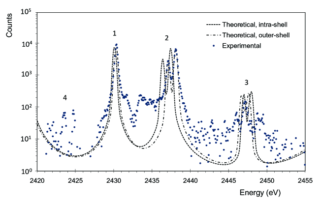
Figure 1: Theoretical spectra for K excitation and single K ionization processes obtained with intra-shell (- - -) and outer-shell correlation (- $\cdot$ -) plotted against experimental data ($\bullet$). The peak 1 refers to the M1 1s 2s ³S₁ $\to$ 1s² line, the peaks 2 and 3 have contributions from the 1s 2s 2p ²P_1/2,3/2 $\to$ 1s² 2s and the 1s 2p ³P₁ $\to$ 1s² lines, and the peak 4 refers to the 1s 2s 2p^{2 3}S₁ $\to$ 1s² 2s 2p ³P_0,1,2 lines.

In a preliminary calculation, we have used the MCDF code, including only intra-shell correlation, to calculate the energies of these lines in the same way as in our previous calculations for Ar ions spectra Martins et al. (2001). The basis space includes all possible electron configurations built from $1s$, $2s$, and $2p$ orbitals corresponding to single and double excitations from the main configuration. The experimental spectrum energy scale has been fixed by setting the He-like $1s2s\,^{3}S_{1}\to 1s^{2}\,{}^{1}S_{0}$ M1 transition to $2430.351\text{\,}\mathrm{e}\mathrm{V}$, using the high-precision QED calculation from Ref. Artemyev et al. (2005). In this case the theoretical results differ from the experimental ones by $0.46\text{\,}\mathrm{e}\mathrm{V}$ and $0.41\text{\,}\mathrm{e}\mathrm{V}$ for the two Li-like lines, respectively, as shown in Tab. 1 and in Fig. 1. These discrepancies are due to the higher accuracy of the present experimental data. Moreover the improved resolution ($0.3\text{\,}\mathrm{e}\mathrm{V}$) in comparison with the Ar case ($3\text{\,}\mathrm{e}\mathrm{V}$) makes the comparison between theoretical and experimental spectra more sensitive to shifts. Therefore a new calculation was performed, including correlation up to the $4f$ sub-shell. For that purpose, the basis space was enlarged to include now all orbitals in the $n=3,4$ electronic shells. A much better agreement with experiment is obtained (see Tab. 1), as the energy differences between theory and experiment were reduced to $0.06\text{\,}\mathrm{e}\mathrm{V}$ and $0.04\text{\,}\mathrm{e}\mathrm{V}$, respectively, for the two Li-like lines, thus showing the importance of electronic correlation in the interpretation of high resolution experiments. We are dealing here with auto-ionizing initial states in these transitions, except in the case of heliumlike line. An auto-ionizing state correspond to a resonance degenerate with a continuum, corresponding to a final state with a free electron, which lead to both a broadening (due to the Auger transition probability) and a shift. Up to now this shift has been evaluated only for neutral atoms with an inner-shell hole Indelicato et al. (1998); Deslattes et al. (2003). Here, a rough estimate of this effect shows it must be in the order of a few meV to a few tenth of eV, depending on the number of allowed Auger channels.

Using our calculation, including only correlation up to $n=4$, we obtain for the M1 line the energy $2430.28\text{\,}\mathrm{e}\mathrm{V}$, $0.07\text{\,}\mathrm{e}\mathrm{V}$ below the experimental value. A more accurate energy shift could be deduced, if the experiment was calibrated against our MCDF value, as some cancellations in the correlation energy should occur: both the initial and final states of the main Li-like transitions, for example, correspond to the M1 line initial and final states with an extra electron.

III.3 Excited species production

Radiative spectra obtained in ECRIS systems usually include radiative lines resulting from de-excitation of ions in different charge states and different levels. A detailed analysis of the main processes leading to those initial states is needed. We refer the reader to Martins et al. Martins et al. (2001) for details.

We assume that all S^q+ ions, where $q$ is the degree of ionization ($q=Z-m$, $m$ being the number of electrons in the ion), are initially in the ground configuration. The two main processes leading to a hole in the K shell are K ionization of the S^(q-1)+ ion ground configuration and excitation of the S^q+ ion ground configuration. In order to generate a preliminary theoretical spectrum, we took into account processes that create single K-hole excited states with two, three, and four electrons from the ground configurations of sulphur ions.

The intensity of the line corresponding to a transition from level $i$ to a level $j$ in a S^q+ ion with a K hole and in level $i$, is given by

$$I_{ij}^{q}=\hbar\omega A_{ij}^{q}N_{i}^{\textrm{\tiny K},q}.$$ (8)

In this equation $\hbar\omega$ and $A_{ij}^{q}$ are the radiative $i\to j$ transition energy and probability, respectively, and $N_{i}^{\textrm{\tiny K},q}$ is the density of S^q+ ions with a K hole and in level $i$. This density is obtained from the balance equation

$$N_{0}^{q}\left\langle N_{e}v_{e}\sigma_{i}^{\textrm{\tiny K-exc,}q}\right\rangle+N_{0}^{q-1}\left\langle N_{e}v_{e}\sigma_{i}^{\textrm{\tiny K-ion,}\left(q-1,q\right)}\right\rangle=N_{i}^{\textrm{\tiny K},q}A_{i}^{q}.$$ (9)

Here, $N_{e}$ is the electron density, $N_{0}^{q}$ and $N_{0}^{q-1}$ are the densities of S^q+ and S^(q-1)+ ions, respectively, in the ground configuration, $A_{i}^{q}$ is the transition probability for de-excitation of these ions by all possible processes (radiative and radiationless), $\sigma_{i}^{\mathrm{K-exc},q}$ is the excitation cross section for the processes leading from the S^q+ ion in the ground configuration to the excited level $i$ of the same ion with a K hole, and $\sigma_{i}^{\mathrm{K-ion},\left(q-1,q\right)}$ is the ionization cross section leading from the S^(q-1)+ ion in the ground configuration to the excited level $i$ of the S^q+ ion with a K hole.

The quantities $\langle N_{e}v_{e}\sigma_{i}\rangle$ give the rate of the number of events related to a process (excitation or ionization), averaged over the electron distribution energy, and are defined by

$$\langle N_{e}v_{e}\sigma_{i}\rangle=N_{e}\int_{E_{min}}^{\infty}f_{e}(E)v_{e}(E)\sigma(E)dE,$$ (10)

where $f_{e}(E)$ is the electron distribution energy, and $v_{e}(E)$ and $\sigma(E)$ are, respectively, the electron velocity, and the cross section for the process, for electron energy $E$.

Electron-impact excitation cross sections were computed using the first Born approximation following the work of Kim et al. Kim and Cheng (1978); Kim and Inokuti (1971). In these calculations we obtained the cross sections for the processes leading from each level $j$ of the S^q+ ion ground configuration, to the excited level $i$ of the S^q+ ion with a K-shell hole, $\sigma_{ji}$. We used a Multi-Configuration Dirac-Fock (MCDF) wave function for the atom and a Dirac wave function for the free electron. Only the Coulomb interaction between the free electron and the atomic electrons was considered. The individual cross sections thus obtained were then weighted by the statistical weight $g_{j}$ of each $j$ level of the ground configuration in order to obtain the excitation cross section $\sigma_{i}^{\mathrm{K-exc},q}$.

K-shell ionization cross-sections were computed using the relativistic binary-encounter-dipole (RBED) model Kim et al. (2000). This method has provided accurate results Santos et al. (2003), even at energies close to the ionization threshold. We use a simplified version of this method, referred as the relativistic binary-encounter-Bethe (RBEB) model, in which, besides the incident electron kinetic energy $T$, only three orbital constants are needed: the kinetic energy of the ejected electron $U$, the orbital binding energy $B$, and the electron occupation number $N$ for the pertinent shell. The RBEB cross section expressions reads

$$\sigma_{\rm RBEB} = \frac{4\pi a_{0}^{2}\alpha^{4}N}{(\beta_{t}^{2}+\beta_{u}^{2}+\beta_{b}^{2})2b^{\prime}}\left\{\frac{1}{2}\left[\ln\left(\frac{\beta_{t}^{2}}{1-\beta_{t}^{2}}\right)-\beta_{t}^{2}-\ln(2b^{\prime})\right]\left(1-\frac{1}{t^{2}}\right)\right.$$ (11)

$$+ \left.1-\frac{1}{t}-\frac{\ln t}{t+1}\frac{1+2t^{\prime}}{(1+t^{\prime}/2)^{2}}+\frac{b^{\prime 2}}{(1+t^{\prime}/2)^{2}}\frac{t-1}{2}\right\}\ .$$

where $t=T/B,\ u=U/B$, $v_{t}$ is the speed of an electron with kinetic energy $T$, $v_{b}$ is the speed of an electron with kinetic energy $B$, $v_{u}$ is the speed of an electron with kinetic energy $U$, $\alpha$ is the fine-structure constant, $a_{0}$ (0.529 Å) is the Bohr radius and

$$\beta_{t}=v_{t}/c,\ \ \ \ \beta_{t}^{2}=1-\frac{1}{(1+t^{\prime})^{2}},\ \ \ \ t^{\prime}=T/mc^{2},$$ (12)

$$\beta_{b}=v_{b}/c,\ \ \ \ \beta_{b}^{2}=1-\frac{1}{(1+b^{\prime})^{2}},\ \ \ \ b^{\prime}=B/mc^{2},$$ (13)

$$\beta_{u}=v_{u}/c,\ \ \ \ \beta_{u}^{2}=1-\frac{1}{(1+u^{\prime})^{2}},\ \ \ \ u^{\prime}=U/mc^{2}.$$ (14)

The product of the ionization cross section, leading from the S^(q-1)+ ion in the ground configuration to the S^q+ ion with a K hole, by the statistical weight $g_{i}$ of the level $i$, yields the K-shell ionization cross section $\sigma_{i}^{\mathrm{K-ion},\left(q-1,q\right)}$ leading from the S^(q-1)+ ion in the ground configuration to the excited level $i$ of the S^q+ ion with a K hole. We assumed a statistical population for each level (with a particular $J$ value) in the final configuration.

As the electron energy distribution is not known, we used Eq. (8) and (9), with cross sections computed by us. We assumed an electron energy distribution which is a linear combination of a Maxwellian distribution (90%), describing the cold electrons at the thermodynamical temperature ($kT$=$1\text{\,}\mathrm{k}\mathrm{e}\mathrm{V}$), and a non-Maxwellian distribution (10%), describing the hot electrons ($kT$=$20\text{\,}\mathrm{k}\mathrm{e}\mathrm{V}$) heated by electron cyclotron resonance Pras et al. (1998). Details of the calculation will be given elsewhere. The ion densities provided by Douysset et al.  Douysset et al. (2000) for the corresponding Ar ions were used as starting values. We note that the initial level of the He-like M1 transition originates from the $1s^{2}$ He-like ions ground configuration by excitation and from the $1s^{2}2s$ Li-like ions ground configuration by single ionization. The initial levels of the two E1 Li-like transitions also originate from the same configuration by excitation.

Although the theoretical spectrum thus obtained spans the 2378–$2460\text{\,}\mathrm{e}\mathrm{V}$ energy range, it is shown in Fig. 1 in the 2420–$2455\text{\,}\mathrm{e}\mathrm{V}$ energy range for comparison with experimental data (dash-dotted line.) The calculated spectrum is normalized to the $2438\text{\,}\mathrm{e}\mathrm{V}$ peak intensity. As Fig. 1 shows, the theoretical spectrum resulting from excited states obtained from the ion ground states by excitation and single K-ionization processes only is enough to account for the major features in the experimental spectrum. In Tab. 2 we list the ion densities used in the theoretical spectrum, obtained through an iterative adjustment to the experimental spectrum.

From the comparison with experiment we note that, although the Li-like line intensities are well reproduced, the M1 He-like line theoretical intensity falls below the experimental intensity. At the same time, some minor features remain unexplained. So, we looked for processes that could lead to other excited states suceptible of explaining the discrepancies between our calculated values and the experimental data.

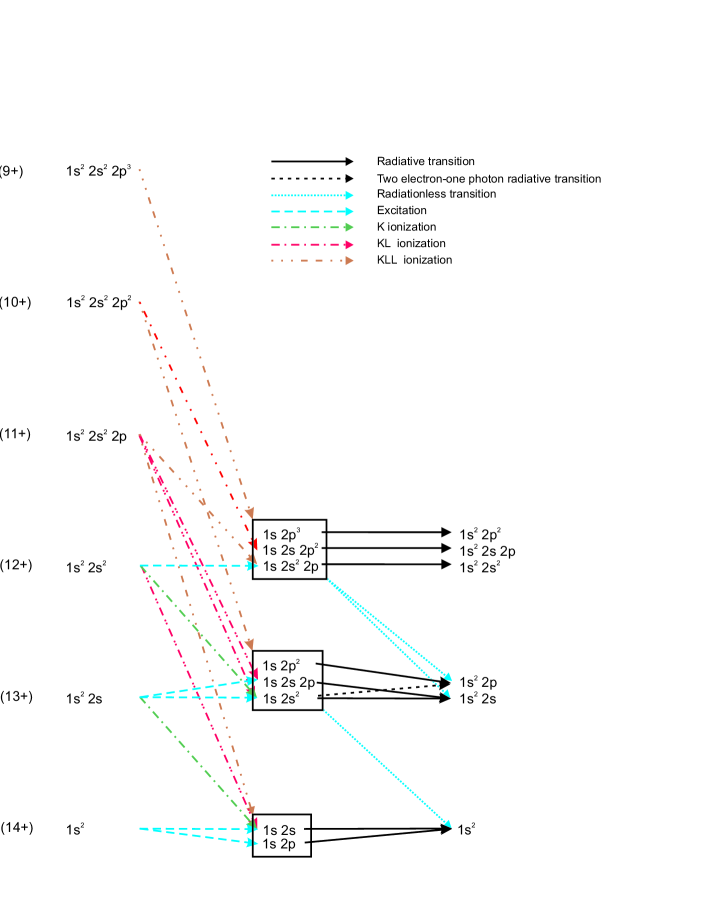
Figure 2: Excitation, ionization and decay processes considered in this work: K excitation (- - -); single K ionization (– $\cdot$ –); double KL ionization (– $\cdot$ $\cdot$ –); triple KLL ionization(– $\cdot$ $\cdot$ $\cdot$ –); radiative decay (—), and radiationless decay($\cdot$ $\cdot$ $\cdot$).

We found out that contributions from the following configurations had also to be included: S¹³⁺ $1s2p^{2}$, and S¹²⁺ $1s2s2p^{2}$, and $1s2p^{3}$. We took into account all excitation, single-ionization, double KL-ionization and triple KLL-ionization processes from the ground state of S⁹⁺ to S¹⁴⁺ ions, leading to these configurations. A diagram of all excitation, ionization and decay processes considered in this work is shown in Fig. 2.

As an example, the S¹²⁺ $1s2s^{2}2p\,^{1}P_{1}$ excited configuration can be obtained through $1s\to 2p$ excitation from the S¹²⁺ 1s² 2s² configuration, through K ionization from the S¹¹⁺ $1s^{2}2s^{2}2p$ configuration, through KL double-ionization from the S¹⁰⁺ $1s^{2}2s^{2}2p^{2}$ configuration, and through KLL triple-ionization from the S⁹⁺ $1s^{2}2s^{2}2p^{3}$ configuration.

In what concerns the calculation of the double KL and triple KLL ionization cross-sections, we used the semi-empirical formula developed by Shevelko and Tawara Shevelko and Tawara (1995), with the fitting parameters proposed by Bélenger et al. B lenger et al. (1997), and the ionization energies calculated in this work (see Tab. 3).

Taking in account all the referred processes, Eq. (8) now reads

$$I_{ij}^{q} = N_{e}\hbar\omega\frac{A_{ij}^{q}}{A_{i}^{q}}\left[N_{0}^{q}\left\langle v\sigma_{i}^{\textrm{\tiny K-exc,}q}\right\rangle+N_{0}^{q-1}\left\langle v\sigma_{i}^{\textrm{\tiny K-ion,}(q-1,q)}\right\rangle\right.$$

$$+ \left.N_{0}^{q-2}\left\langle v\sigma_{i}^{\textrm{\tiny KL-ion,}(q-2,q)}\right\rangle+N_{0}^{q-3}\left\langle v\sigma_{i}^{\textrm{\tiny KLL-ion,}(q-3,q)}\right\rangle\right].$$

In this equation, $\sigma_{i}^{\textrm{\tiny KL-ion,}(q-2,q)}$ and $\sigma_{i}^{\textrm{\tiny KLL-ion,}(q-3,q)}$ are the double and triple ionization cross sections respectively.

IV Results and discussion

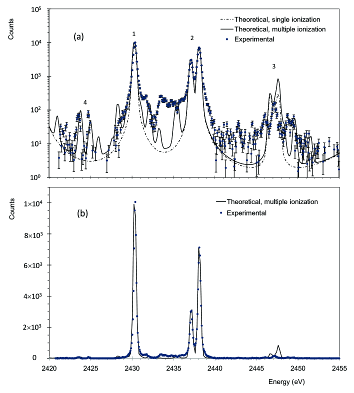
Figure 3: Theoretical spectra obtained with single ionization (- $\cdot$ -) and multiple ionization (—) processes plotted against experimental data ($\bullet$) in log scale (a) and linear sclae (b). For the legend of the peaks, see Fig. 1 caption.

The theoretical spectrum, including all lines resulting from the decay of the excited states shown in Fig. 2, obtained using the methods discussed above and assuming, for each line, a linear combination of a gaussian and a lorentzian distributions, designed to approximate a Voigt profile with $0.3\text{\,}\mathrm{e}\mathrm{V}$ width, is presented in Fig. 3 in a semilogarithmic scale(a), and in a linear scale(b). In Fig. 3(a) is shown, as a dash-dotted line, the theoretical spectrum resulting from excited states obtained from the ion ground states by excitation and single K-ionization processes only. This is enough to account for the major features in the experimental spectrum, clearly seen in Fig. 3(b). Therefore we looked for other processes that could lead to new excited states also from the ground states. Fig. 3(a) shows that inclusion of double-KL and triple-KLL ionization allows for a much better theoretical interpretation of these features.

If only single ionization and excitation processes are considered, the $1s^{2}2s$ and $1s^{2}$ ground configurations are the only ones that contribute to the experimental sulphur spectrum in the 2420–$2455\text{\,}\mathrm{e}\mathrm{V}$ energy range, the first one through single ionization, and the second one through monopole excitation.

In this case, the $2446.68\text{\,}\mathrm{e}\mathrm{V}$ and $2448.28\text{\,}\mathrm{e}\mathrm{V}$ lines, resulting from the decay of the $1s2p\,^{3}P_{1,2}$ levels are not significant, as these levels are poorly fed by single excitation from the $1s^{2}$ ground configuration. Also based in the single excitation and ionization processes, the calculated intensity of the M1 line resulting from de-excitation of the $1s2s\,^{3}S_{1}$ level is lower than the corresponding experimental line intensity, after adjusting the calculated spectrum to the $2438\text{\,}\mathrm{e}\mathrm{V}$ line intensity.

However, the $1s2s$ configuration may also be obtained through double- and triple-ionization processes, from the $1s^{2}2s^{2}$ and $1s^{2}2s^{2}2p$ configuration states, respectively. Including the contribution of these processes in the calculated spectra allows for a much better fit to the experimental spectra.

The intensity ratio between the M1 $1s2s\,^{3}S_{1}\to 1s^{2}\,{}^{1}S_{0}$ and the $1s2s2p\,^{2}P_{3/2}\to 1s^{2}2s\,^{2}S_{1/2}$ lines (denoted 1 and 2 in Fig. 1) is given by

$$\frac{I_{1}}{I_{2}}=\frac{\left[[N^{14+}\sigma^{\textrm{\tiny{exc}}}_{\textrm{\tiny{K$\to$ L}}}({1s}^{2}\to{1s2s})+N^{13+}\sigma^{\textrm{\tiny{ion}}}_{\textrm{\tiny{K}}}({1s}^{2}{2s}\to{1s2s})+N^{12+}\sigma^{\textrm{\tiny{ion}}}_{\textrm{\tiny{KL}}}({1s}^{2}{2s}^{2}\to{1s2s})\right]TY_{1}}{N^{13+}\sigma^{\textrm{\tiny{exc}}}_{\textrm{\tiny{K$\to$ L}}}({1s}^{2}{2s}\to{1s2s2p}\,^{2}{P}_{3/2})TY_{2}}\times g({1s2s}\,^{3}{S}_{1}).$$ (16)

Here $N^{q+}$ are the densities of S^q+ ion in the ground configuration and $g$ is the statistical weight of the $1s2s\ ^{3}S_{1}$ level, and $TY_{i}$ is the transition yield of line $i$.

The $1s2s2p^{2}$ ion configuration is obtained when the double KL and triple KLL ionization processes are taken in account. The $1s2s2p^{2}\,{}^{3}S_{1}\to 1s^{2}2s2p\,^{3}P_{J}$, $J=0,1,2$ triplet visible at the left in the figure in now predicted in agreement with experiment.

One should note that there are several weak features in the spectrum in Fig. 3, which are not reproduced. These features, are slightly above statistical noise. Some of them could be due to $n=3$ or 4 satellite lines of the heliumlike and lithiumlike ions. Yet our calculations did not produce any line that could explain the observed features. A search in X-ray transition energy database Deslattes et al. (2003) could not produce any line that could explain those features.

The energy and transition yield values calculated in this work for all lines contributing to the theoretical spectrum are listed in Tab. LABEL:tab:ty. The excitation cross sections are shown in Table  5 for $10\text{\,}\mathrm{k}\mathrm{e}\mathrm{V}$ impact energy, as an example.

V Conclusions

Ion densities in the plasma depend on the electron energy distribution. For hot electrons this distribution is non-Maxwellian, making difficult the calculation of the ion densities. So, for the generation of the theoretical spectrum, we started from the ion densities provided by Douysset et al Douysset et al. (2000). Individual line intensities were obtained using Eq. (8) with the cross section values computed by us assuming a linear combination of Maxwellian distribution, describing the cold electrons, and a non-Maxwellian distribution, describing the hot electrons, and the estimated ion densities. After comparison with the experimental spectrum, ion densities were then adjusted in order to match the experimental peak intensities. In this way we were able to obtain a reasonable agreement between theory and experiment.

In this work we have shown evidence of the contribution of several new mechanism that contribute to the creation of excited state in an ECRIS plasma. In particular double and triple processes must be considered to reproduce properly line intensities. We have also shown that MCDF transition energies with medium size configuration space can reproduce reasonably well most features of the spectra, including energies and branching ratios. In some part of the spectrum there are hint of weak lines that could not be reproduced so far, despite extensive search, including $n=3$ satellites of heliumlike and lithiumlike lines.

Table 1: Electronic correlation effect on the 1s 2s ³S₁ $\to$ 1s^{2 1}S₀ M1 line energy and on the energy shifts, relative to the M1 line, of the 1s 2s 2p ²P_1/2 $\to$ 1s² 2s E1(1) and 1s 2s 2p ²P_3/2 $\to$ 1s² 2s E1(2) lines, compared to experiment. The energy values are in eV.

	M1	E1 (1)	E1 (2)
Intra-shell correlation (up to 2p)	2430.09	6.30	7.34
Outer-shell correlation (up to 4f)	2430.29	6.82	7.79
Experiment		6.76	7.75

Table 2: Ion density values obtained through an iterative adjustment to the experimental spectrum.

	Ion densities (m-3)
S9+	$8.0\times^{15}$
S10+	$7.0\times^{15}$
S11+	$7.0\times^{15}$
S12+	$9.0\times^{15}$
S13+	$1.4\times^{15}$
S14+	$7.0\times^{15}$

Table 3: Calculated energies for single K- (1s^-1), double KL- (1s^-1 2s^-1, 1s^-1 2p^-1) and triple KLL- (1s^-1 2s^-2) ionization (in eV).

	Configuration	1s-1	1s-1 2s-1	1s-1 2p-1	1s-1 2s-2
S9+	1s2 2s2 2p3	2799.63	3332.02	3328.31	4344.02
S10+	1s2 2s2 2p2	2880.79	3476.37	3472.45	4608.55
S11+	1s2 2s2 2p	2967.42	3626.01	3619.21	4869.29
S12+	1s2 2s2	3059.32	3787.89		5141.14
S13+	1s2 2s	3135.92	3929.29
S14+	1s2	3222.42

Table 4: Energy and Transition yield ($TY$) values calculated in this work for all lines contributing to the theoretical spectrum.

$q$	confi	$LSJ_{i}$	conff	$LSJ_{f}$	$E$ (eV)	$TY$
13+	1s 2s2	2S1/2	1s2 2p	2P3/2	2378.45	1.75E-02
13+	1s 2s2	2S1/2	1s2 2p	2P1/2	2380.36	1.02E-02
12+	1s 2p3	5S2	1s2 2p2	3P2	2387.45	1.06E-03
12+	1s 2p3	5S2	1s2 2p2	3P1	2388.45	7.10E-04
12+	1s 2p3	3D3	1s2 2p2	1D2	2397.23	1.97E-03
12+	1s 2p3	3D3	1s2 2p2	3P2	2404.12	1.27E-01
12+	1s 2p3	1P1	1s2 2p2	1S0	2404.20	3.39E-01
12+	1s 2p3	3D2	1s2 2p2	3P2	2404.39	7.82E-02
12+	1s 2p3	3D1	1s2 2p2	3P2	2404.39	8.66E-03
12+	1s 2s 2p2	1D2	1s2 2s 2p	1P1	2405.31	3.93E-01
12+	1s 2p3	3D2	1s2 2p2	3P1	2405.40	3.80E-01
12+	1s 2p3	3D1	1s2 2p2	3P1	2405.40	1.29E-01
12+	1s 2s2 2p	3P1	1s2 2s2	1S0	2405.75	3.37E-03
12+	1s 2s 2p2	3P1	1s2 2s 2p	1P1	2406.00	3.82E-02
12+	1s 2p3	3D1	1s2 2p2	3P0	2406.04	2.31E-01
12+	1s 2s 2p2	3P2	1s2 2s 2p	1P1	2407.05	1.93E-01
12+	1s 2p3	1D2	1s2 2p2	1D2	2408.18	7.78E-01
12+	1s 2p3	3S1	1s2 2p2	3P2	2409.99	3.73E-01
12+	1s 2p3	3P2	1s2 2p2	1D2	2410.23	2.99E-01
12+	1s 2p3	3S1	1s2 2p2	3P1	2411.00	2.82E-01
12+	1s 2s 2p2	3D3	1s2 2s 2p	3P2	2411.10	3.28E-01
12+	1s 2s 2p2	3D2	1s2 2s 2p	3P1	2411.41	2.94E-01
12+	1s 2p3	3S1	1s2 2p2	3P0	2411.64	9.44E-02
12+	1s 2s 2p2	3P1	1s2 2s 2p	3P2	2412.07	2.75E-01
12+	1s 2s 2p2	3D2	1s2 2s 2p	3P2	2412.22	9.74E-03
12+	1s 2s 2p2	3P0	1s2 2s 2p	3P1	2412.29	5.29E-01
12+	1s 2s 2p2	3D1	1s2 2s 2p	3P2	2412.39	1.39E-01
12+	1s 2s 2p2	3P2	1s2 2s 2p	3P2	2413.04	8.62E-01
12+	1s 2s 2p2	3P1	1s2 2s 2p	3P1	2413.27	3.83E-01
12+	1s 2s 2p2	3D1	1s2 2s 2p	3P1	2413.36	2.70E-01
12+	1s 2s 2p2	3P2	1s2 2s 2p	3P1	2414.23	2.76E-02
12+	1s 2s 2p2	3P1	1s2 2s 2p	3P0	2414.24	3.69E-02
12+	1s 2p3	1D2	1s2 2p2	3P2	2415.07	1.75E-01
13+	1s 2s 2p	4P1/2	1s2 2s	2S1/2	2415.18	5.28E-01
13+	1s 2s 2p	4P3/2	1s2 2s	2S1/2	2415.69	2.14E-02
12+	1s 2s 2p2	1P1	1s2 2s 2p	1P1	2416.02	9.80E-01
12+	1s 2p3	1D2	1s2 2p2	3P1	2416.07	1.66E-02
12+	1s 2p3	3P1	1s2 2p2	3P2	2416.49	5.44E-01
13+	1s 2s 2p	4P5/2	1s2 2s	2S1/2	2416.93	1.21E-01
13+	1s 2p2	4P5/2	1s2 2p	2P3/2	2417.01	9.90E-01
12+	1s 2p3	3P2	1s2 2p2	3P2	2417.13	1.06E-01
13+	1s 2p2	4P1/2	1s2 2p	2P1/2	2417.16	9.29E-03
12+	1s 2p3	3P1	1s2 2p2	3P1	2417.49	1.26E-01
12+	1s 2p3	3P0	1s2 2p2	3P1	2417.56	1.00E+00
12+	1s 2p3	3P2	1s2 2p2	3P1	2418.13	3.24E-02
12+	1s 2p3	3P1	1s2 2p2	3P0	2418.14	1.46E-01
12+	1s 2s 2p2	1S0	1s2 2s 2p	1P1	2418.49	4.64E-01
12+	1s 2s2 2p	1P1	1s2 2s2	1S0	2418.58	3.41E-01
12+	1s 2p3	1P1	1s2 2p2	1D2	2420.98	3.85E-01
12+	1s 2s 2p2	3S1	1s2 2s 2p	3P2	2423.78	3.72E-01
12+	1s 2s 2p2	3S1	1s2 2s 2p	3P1	2424.97	1.80E-01
12+	1s 2s 2p2	3S1	1s2 2s 2p	3P0	2425.94	5.06E-02
12+	1s 2s 2p2	1D2	1s2 2s 2p	3P2	2427.61	1.50E-02
12+	1s 2s 2p2	3P1	1s2 2s 2p	3P2	2428.29	6.35E-01
12+	1s 2s 2p2	3P0	1s2 2s 2p	3P1	2428.68	8.25E-02
12+	1s 2s 2p2	3P2	1s2 2s 2p	3P2	2429.35	1.19E-01
12+	1s 2s 2p2	3P1	1s2 2s 2p	3P1	2429.48	2.85E-02
14+	1s 2s	3S1	1s2	1S0	2430.29	1.00E+00
12+	1s 2s 2p2	3P1	1s2 2s 2p	3P0	2430.45	6.82E-02
12+	1s 2s 2p2	3P2	1s2 2s 2p	3P1	2430.54	2.88E-02
13+	1s 2p2	2D5/2	1s2 2p	2P3/2	2431.02	3.53E-01
13+	1s 2p2	2D3/2	1s2 2p	2P1/2	2432.09	9.94E-01
13+	1s 2p2	2P1/2	1s2 2p	2P3/2	2433.28	2.80E-01
13+	1s 2p2	2P1/2	1s2 2p	2P1/2	2435.19	6.57E-01
13+	1s 2p2	2P3/2	1s2 2p	2P3/2	2435.49	9.22E-01
13+	1s 2s 2p	2P1/2	1s2 2s	2S1/2	2437.11	9.39E-01
13+	1s 2p2	2P3/2	1s2 2p	2P1/2	2437.40	7.83E-02
13+	1s 2s 2p	2P3/2	1s2 2s	2S1/2	2438.08	1.00E+00
14+	1s 2p	3P1	1s2	1S0	2446.68	1.00E+00
13+	1s 2s 2p	2P1/2	1s2 2s	2S1/2	2447.24	3.24E-01
13+	1s 2s 2p	2P3/2	1s2 2s	2S1/2	2447.64	9.06E-01
14+	1s 2p	3P2	1s2	1S0	2448.28	3.10E-01
13+	1s 2p2	2S1/2	1s2 2p	2P3/2	2449.62	6.60E-01
13+	1s 2p2	2S1/2	1s2 2p	2P1/2	2451.53	1.89E-01
14+	1s 2p	1P1	1s2	1S0	2460.15	1.00E+00

Table 5: Sulphur ions excitation cross sections, for 10 keV electron impact energy.

$q$	initial conf.		final conf.		$\sigma$ (m2)
$12^{+}$	1s2 2s2	1S0	1s 2s2 2p	3P1	$2.05\times 10^{-27}$
				1P1	$3.05\times 10^{-25}$
$13^{+}$	1s2 2s	2S1/2	1s 2s2	2S1/2	$1.96\times 10^{-26}$
			1s 2s 2p	4P1/2	$6.68\times 10^{-29}$
				2P${}_{1/2}^{(2)}$	$1.62\times 10^{-25}$
				2P${}_{1/2}^{(1)}$	$1.64\times 10^{-26}$
				4P3/2	$3.68\times 10^{-28}$
				2P${}_{3/2}^{(1)}$	$3.45\times 10^{-25}$
				2P${}_{3/2}^{(2)}$	$1.06\times 10^{-26}$
$14^{+}$	1s2	1S0	1s 2p	3P1	$2.29\times 10^{-27}$
				1P1	$3.21\times 10^{-25}$
				3S1	$3.72\times 10^{-26}$