Yukawa Couplings and Quark and Lepton Masses in an $SO(10)$ Model with a Unified Higgs Sector

Pran Nath^a and Raza M. Syed^b

a. Department of Physics, Northeastern University, Boston, MA 02115-5000, USA
b. Department of Physics, American University of Sharjah, P.O. Box 26666, Sharjah, UAE

Abstract

An analytic computation is given of the generation of Yukawa couplings and of the quark, charged lepton and neutrino masses in the framework of an $SO(10)$ model with a unified Higgs sector consisting of a single pair of vector-spinor $144+\overline{144}$ of Higgs multiplets. This unified Higgs sector allows for a breaking of $SO(10)$ to the gauge group $SU(3)\times SU(2)_{L}\times U(1)_{Y}$ and contains light Higgs doublets allowing for the breaking of the electroweak symmetry. Fermion mass generation in this model typically arises from quartic couplings $16\cdot 16\cdot 144\cdot 144$ and $16\cdot 16\cdot\overline{144}\cdot\overline{144}$. Extending a previous work it is shown that much larger third generation masses can arise for all the fermions from mixing with $45$ and $120$ matter multiplets via the cubic couplings $16\cdot 45\cdot\overline{144}$ and $16\cdot 120\cdot 144$. Further it is found that values of $\tan\beta$ as low as 10 can allow for a $b-\tau-t$ unification consistent with current data. The quartic and cubic couplings naturally lead to Dirac as well as Majorana neutrino masses necessary for the generation of See Saw neutrino masses.

1 Introduction

Over the recent past the gauge group $SO(10)$ has emerged as the leading candidate for the unification of forces including the strong, the weak and the electromagnetic[1], and at the same time the $16$ plet representation of $SO(10)$ can accommodate a full generation of quarks and leptons. Further, the singlet in the $16$ plet is identified as a right handed neutrino which can combine with the left handed neutrino in the $16$ plet to generate a Dirac mass and at the same time if the singlet acquires a large Majorana mass, one can generate small neutrino masses by the well known See Saw mechanism. While this is a very nice picture, an actual implementation of an $SO(10)$ grand unification requires many Higgs multiplets for the explicit breaking of the gauge symmetry down to its residual $SU(3)_{C}\times U(1)_{\rm em}$ form (For a review see [2]). Thus, for example, a possible breaking scheme discussed in the literature is to use a $45$ plet of Higgs to break $SO(10)$, a $16+\overline{16}$ to reduce the rank of the gauge group and $10$ plets of Higgs to break the electroweak symmetry. Many other schemes involving several Higgs multiplets for the breaking of $SO(10)$ to its residual $SU(3)_{C}\times U(1)_{\rm em}$ have also been discussed.

Recently a new formalism was proposed which has a unified Higgs structure, i.e., a $144+\overline{144}$ multiplets of Higgs [3, 4]. It was shown that the above Higgs structure can break $SO(10)$ and and reduce the rank of the gauge group at the same time such that $SO(10)\to SU(3)_{C}\times SU(2)\times U(1)_{Y}$ at the GUT scale $M_{G}$. How this comes about can be easily seen by examining the $SU(5)\times U(1)$ decomposition of the $45$ plet and the $144$ plet in representations of $SO(10)$ so that

$$45=1(0)+10(4)+\overline{10}(-4)+24(0),$$

$$144=\bar{5}(3)+5(7)+10(-1)+{15}(-1)+24(-5)+40(-1)+\overline{45}(3).$$ (1)

where the quantity in the parentheses represents the $U(1)$ quantum numbers. For the usual model building where the $45$ plet of Higgs is utilized to break $SO(10)$ it is a combination of the singlet $1(0)$ and the $24(0)$ plets of Higgs that develop VEVs. Since each of these carry no $U(1)$ quantum numbers, giving a VEV to the $45$ plet does not reduce the rank of the group. In the decomposition of $144$ one finds that all the components carry $U(1)$ quantum numbers, and thus a VEV formation in $144$ along the $45$ plet direction not only breaks $SO(10)$ but also reduces the rank of the gauge group and consequently $SO(10)$ breaks directly to the Standard Model gauge group $SU(3)_{C}\times SU(2)_{L}\times U(1)_{Y}$. Further, it was shown in [3, 4] that a pair of light doublets can be gotten which are necessary for the breaking of the electroweak symmetry which occurs when $5,\bar{5},\overline{45}(45)$ components of $144(\overline{144})$ develop vacuum expectation values. With the $144+\overline{144}$ Higgs sector, mass generation for the fermions requires at least the quartic interactions

$$\frac{1}{\Lambda}(16\cdot 16\cdot 144\cdot 144),\leavevmode\nobreak\ \leavevmode\nobreak\ \frac{1}{\Lambda}(16\cdot 16\cdot\overline{144}\cdot\overline{144}).$$ (2)

where $\Lambda$ would typically be of size the string scale $M_{st}$. After spontaneous breaking at the GUT scale the $144$ and $\overline{144}$ will develop a VEV of size $M_{G}$ and the above quartic coupling will lead to Yukawa interactions of matter fields with the Higgs doublets and these Yukawas will be $O(M_{G}/M_{st})$, which are the appropriate size for the Yukawas for the first and for the second generation fermions. One of the aims of the analysis of this work is to compute explicitly these Yukawa couplings. To exhibit this explicitly we expand the $16$ plet of matter fields in $SU(5)\times U(1)$ decomposition so that

$$16=1(-5)+\bar{5}(3)+10(-1).$$ (3)

It is then easily seen that interactions of Eq.(2) produce the Yukawa couplings necessary for generating the masses for the up quarks, the down quarks and the charged leptons, and also give couplings which generate Dirac and Majorana masses for the neutrinos. We list these below in the $SU(5)\times U(1)$ decomposition indicating the light doublet ${\mathsf{D}}_{1}$, ${\mathsf{D}}_{2}$ or ${\mathsf{D}}_{3}$ for which the specific interaction listed below is valid

$$\underline{{\rm From\leavevmode\nobreak\ quartic\leavevmode\nobreak\ couplings}\leavevmode\nobreak\ 16\cdot 16\cdot 144\cdot 144}$$

$${u-\rm quarks}: \frac{1}{\Lambda}10_{16}(-1)\cdot 10_{16}(-1)\cdot<5_{144}(7)\cdot 24_{144}(-5)>\leavevmode\nobreak\ ({\mathsf{D}}_{1}),$$ (4)

$${d-\rm quarks+leptons}: \frac{1}{\Lambda}\bar{5}_{16}(3)\cdot 10_{16}(-1)\cdot<\bar{5}_{144}(3)\cdot 24_{144}(-5)>\leavevmode\nobreak\ ({\mathsf{D}}_{2},{\mathsf{D}}_{3}),$$ (6)

$$\frac{1}{\Lambda}\bar{5}_{16}(3)\cdot 10_{16}(-1)\cdot<{\overline{45}}_{144}(3)\cdot 24_{144}(-5)>\leavevmode\nobreak\ ({\mathsf{D}}_{2},{\mathsf{D}}_{3}),$$

$${LR}-\nu{\rm\leavevmode\nobreak\ mass}: \frac{1}{\Lambda}1_{16}(-5)\cdot\bar{5}_{16}(3)\cdot<5_{144}(7)\cdot 24_{144}(-5)>\leavevmode\nobreak\ ({\mathsf{D}}_{1}),$$ (7)

$${RR}-\nu{\rm\leavevmode\nobreak\ mass}: {\rm None},$$ (8)

$${LL}-\nu{\rm\leavevmode\nobreak\ mass}: \bar{5}_{16}(3)\cdot\bar{5}_{16}(3)\cdot 15_{144}(-1)\cdot 24_{\overline{144}}(-5)\leavevmode\nobreak\ ({\mathsf{D}}_{1},{\mathsf{D}}_{2},{\mathsf{D}}_{3}),$$ (9)

where $10_{16}(-1)$ etc. stand for the $10$ plet of $SU(5)$ arising from the $16$ plet of $SO(10)$ and $(-1)$ is the $U(1)$ charge in the $SO(10)\to SU(5)\times U(1)$ decomposition etc..

$$\underline{{\rm From\leavevmode\nobreak\ quartic\leavevmode\nobreak\ couplings}\leavevmode\nobreak\ 16\cdot 16\cdot\overline{144}\cdot\overline{144}}$$

$${u-\rm quarks:} \frac{1}{\Lambda}10_{16}(-1)\cdot 10_{16}(-1)\cdot<5_{\overline{144}}(-3)\cdot 24_{\overline{144}}(5)>\leavevmode\nobreak\ ({\mathsf{D}}_{2},{\mathsf{D}}_{3}),$$ (11)

$$\frac{1}{\Lambda}10_{16}(-1)\cdot 10_{16}(-1)\cdot<{45}_{\overline{144}}(-3)\cdot 24_{\overline{144}}(5)>\leavevmode\nobreak\ ({\mathsf{D}}_{2},{\mathsf{D}}_{3}),$$

$${d-\rm quarks+leptons}: \frac{1}{\Lambda}\bar{5}_{16}(3)\cdot 10_{16}(-1)\cdot<\bar{5}_{\overline{144}}(-7)\cdot 24_{\overline{144}}(5)>\leavevmode\nobreak\ ({\mathsf{D}}_{1}),$$ (12)

$${LR}-\nu{\rm\leavevmode\nobreak\ mass}: \frac{1}{\Lambda}1_{16}(-5)\cdot\bar{5}_{16}(3)\cdot<5_{\overline{144}}(-3)\cdot 24_{\overline{144}}(5)>\leavevmode\nobreak\ ({\mathsf{D}}_{2},{\mathsf{D}}_{3}),$$ (14)

$$\frac{1}{\Lambda}1_{16}(-5)\cdot\bar{5}_{16}(3)\cdot<{45}_{\overline{144}}(-3)\cdot 24_{\overline{144}}(5)>\leavevmode\nobreak\ ({\mathsf{D}}_{2},{\mathsf{D}}_{3}),$$

$${RR}-\nu{\rm\leavevmode\nobreak\ mass}: \frac{1}{\Lambda}1_{16}(-5)\cdot 1_{16}(-5)\cdot<24_{\overline{144}}(5)\cdot 24_{\overline{144}}(5)>\leavevmode\nobreak\ ({\mathsf{D}}_{1},{\mathsf{D}}_{2},{\mathsf{D}}_{3}),$$ (15)

$${LL}-\nu{\rm\leavevmode\nobreak\ mass}: \frac{1}{\Lambda}\bar{5}_{16}(3)\cdot\bar{5}_{16}(3)\cdot<5_{\overline{144}}(-3)\cdot 5_{\overline{144}}(-3)>\leavevmode\nobreak\ ({\mathsf{D}}_{2},{\mathsf{D}}_{3}),$$ (17)

$$\frac{1}{\Lambda}\bar{5}_{16}(3)\cdot\bar{5}_{16}(3)\cdot<{45}_{\overline{144}}(-3)\cdot{45}_{\overline{144}}(-3)>\leavevmode\nobreak\ ({\mathsf{D}}_{2},{\mathsf{D}}_{3}).$$

After spontaneous breaking at the GUT scale the Higgs multiplets $24_{H}$ develop a VEV of size $M_{G}$ generating Yukawa couplings for the quarks and the leptons of size $O(M_{G}/\Lambda)$ followed by a spontaneous symmetry breaking at the electroweak scale which give VEVs to the Higgs doublets and generate quark and lepton masses.

Since $\Lambda$ would be of the size of the string scale ($M_{St}$) the ratio $O(M_{G}/\Lambda)<<1$ is appropriate for the Yukawa couplings for the first two generations of quarks and charged leptons. From Eq.(14) and Eq.(14) one finds that a similar size $LR$ Yukawa coupling arises for the neutrinos. Quite remarkably the same quartic interactions of Eq.(2) lead to large (GUT size) masses needed for the generation of Type I See Saw neutrino masses and very small $LL$ neutrino masses for a Type II See Saw. Thus from Eq.(15) we see that with $M_{G}\sim 10^{16}$ GeV, and $\Lambda\sim 10^{17}$ GeV one finds that $RR$ neutrino masses are $O(M_{G}^{2}/\Lambda)\sim 10^{15}$ GeV. Similarly from Eq.(17) one finds the $LL$ neutrino masses to be of size $O(M_{EW}^{2}/\Lambda)$ which gives $LL$ masses in the range $10^{-3\pm 1}$eV .

We note now the following two possibilities:

1. For the case when $(\bar{5}_{\overline{144}}(-3),5_{144}(3))$ and $(45_{\overline{144}}(-3),\overline{45}_{144}(3))$ contain the light pair of doublets, only the down quark masses will arise from the quartic couplings $16\cdot 16\cdot 144\cdot 144$, while the masses for the up quarks, $LR$-Dirac masses, $LL$ and $RR$ masses for the neutrinos will all arise only from the $16\cdot 16\cdot\overline{144}\cdot\overline{144}$ couplings.
   

2. For the case when $(\bar{5}_{\overline{144}}(-7),5_{144}(7))$ contain the light doublets, the up quark masses and the $LR$-Dirac neutrino masses arise from the quartic couplings $16\cdot 16\cdot 144\cdot 144$, while the masses for the down quark and lepton as well as $RR$ neutrino masses arise from the $16\cdot 16\cdot\overline{144}\cdot\overline{144}$ couplings. Here, however, no $LL$ neutrino masses are generated.

To generate larger Yukawa couplings for the third generation, it was proposed in [4] that one include additional $10$ and $45$ of matter. These allow couplings at the cubic level of the form

$$h^{(10)}_{\acute{a}\acute{b}}16_{\acute{a}}\cdot 144_{\acute{b}}\cdot 10,\leavevmode\nobreak\ \leavevmode\nobreak\ \leavevmode\nobreak\ h^{(45)}_{\acute{a}\acute{b}}16_{\acute{a}}\cdot\overline{144}_{\acute{b}}\cdot 45,$$ (18)

where $\acute{a},\acute{b}$ are the generation indices and where the $SU(5)\times U(1)$ decomposition of $45$ plet is given in Eq.(1), while the $SU(5)\times U(1)$ decomposition of $10$ plet is given by

$$10=\bar{5}(-2)+5(2).$$ (19)

In this case one can define the combination of $16_{\acute{a}}$ that couples with the 10 plet and the 45 plet of matter as the third generation. The production of the third generation fermion masses depends on the choice of the light Higgs doublets. For the light Higgs doublets with $U(1)$ quantum numbers $\pm 3$ mass generation occurs for the b quark, the tau lepton and for the top quark. However, no Dirac mass is generated for the neutrino and thus a neutrino mass generation from a Type I See Saw cannot occur. For another choice of the light Higgs doublets where the $U(1)$ quantum numbers for the doublets are $\pm 7$, one finds that the b quark, and the tau lepton get masses and a Dirac mass is generated for the neutrino, but there is no generation of mass for the top quark. In short it is not possible with a $10$ plet and a $45$ plet of matter to give masses to the up and to the down quarks, to the charged lepton and also give a Dirac mass to the neutrino all at once. To overcome this problem we analyze in this paper the alternate possibility of including a $45$ plet and a $120$ plet of matter fields. Thus as an alternative to Eq.(18) we will consider the cubic couplings

$$h^{(120)}_{\acute{a}\acute{b}}16_{\acute{a}}\cdot 144_{\acute{b}}\cdot 120,\leavevmode\nobreak\ \leavevmode\nobreak\ \leavevmode\nobreak\ h^{(45)}_{\acute{a}\acute{b}}16_{\acute{a}}\cdot\overline{144}_{\acute{b}}\cdot 45,$$ (20)

where the $SU(5)\times U(1)$ decomposition of $120$ is given by

$$120=5(2)+\bar{5}(-2)+10(-6)+\overline{10}(6)+45(2).$$ (21)

The outline of the rest of the paper is as follows: In Sec.(2) we discuss the Higgs sector of $SO(10)$ and the conditions for the spontaneous breaking of $SO(10)$, as well as the generation of light Higgs doublets. In Sec.(3) we compute the Yukawa couplings that arise from the quartic interactions between matter and Higgs fields. Here we also compute quark, charged lepton and neutrino masses arising from the quartic couplings. In Sec.(4) we analyze the cubic couplings that arise from inclusion of $45_{M}$ and $120_{M}$ of matter. In this section we then discuss the production of masses for the third generation fermions from these couplings. In Sec.(5) we give an analysis of $b-\tau-t$ unification. In Sec.(6) we give an analysis of the $\tau$ neutrino mass. Proton stability is briefly discussed in Sec.(7). Conclusions are given in Sec.(8). Further details of the analysis are given in several Appendices which are referred to in the main text of the paper. Thus Appendix A gives a brief discussion of the formalism and of the calculational techniques. Details of the analysis of quartic couplings are given in Appendix B, and the general mass formulae arising from the quartic couplings after spontaneous breaking are given in Appendix C. Appendix D gives details of the analysis of the cubic interactions $16\cdot 45\cdot\overline{144}$ and $16\cdot 120\cdot 144$ while the details of the couplings that generate fermionic masses from cubic couplings are given in Appendix E. Appendix F gives the definitions of various quantities that enter in the diagonalization of the $b.\tau,t$ mass matrices. Finally Appendix G defines the Yukawa coupling parameters that enter in Sec.(4).

2 The Higgs Sector and the Spontaneous Breaking of $SO(10)$

As discussed in [3, 4] spontaneous symmetry breaking in the Higgs sector can be generated by considering the superpotential

$${\mathsf{W}} = M{(\overline{144}_{H}\cdot 144_{H})}+\frac{1}{M^{\prime}}\left[\lambda_{45_{1}}{(\overline{144}_{H}\cdot 144_{H})_{45_{1}}(\overline{144}_{H}\cdot 144_{H})_{45_{1}}}\right.$$ (22)

$$\left.+\lambda_{45_{2}}{(\overline{144}_{H}\cdot 144_{H})_{45_{2}}(\overline{144}_{H}\cdot 144_{H})_{45_{2}}}+\lambda_{210}{(\overline{144}_{H}\cdot 144_{H})_{210}(\overline{144}_{H}\cdot 144_{H})_{210}}\right].$$

We look for solutions where the $24$ plet of $SU(5)$ ${\bf Q}^{i}_{j}$ in the $144$ and the 24-plet of $SU(5)$ ${\bf P}^{i}_{j}$ in $\overline{144}$ (see Appendix A) develop VEVs which preserve the Standard Model gauge group $SU(3)_{C}\times SU(2)_{L}\times U(1)Y$ such that

$$<{\bf Q}^{i}_{j}>=q\leavevmode\nobreak\ \textnormal{diag}(2,2,2,-3,-3),\leavevmode\nobreak\ \leavevmode\nobreak\ <{\bf P}^{i}_{j}>=p\leavevmode\nobreak\ \textnormal{diag}(2,2,2,-3,-3),$$ (23)

which results in the minimization condition for the potential so that

$$\frac{MM^{\prime}}{qp}=116\lambda_{45_{{}_{1}}}+7\lambda_{45_{{}_{2}}}+4\lambda_{210}.$$ (24)

A fine tuning is needed to get a pair of light Higgs doublets so one is working within the framework of a landscape type scenario. As discussed in [4] a light pair of Higgs doublets can be gotten by looking at the mass matrices for the Higgs doublets ${\bf Q}_{a},{\bf\widetilde{Q}}_{a},{\bf P}_{a},{\bf P}^{a},{\bf\widetilde{P}}^{a},{\bf Q}^{a}$ (see Appendix A). Here the $SU(2)$ index $a$ can take on values 4 and 5.

We will denote the fields in the mass diagonal basis with a prime and these are related to the unprimed fields by a unitary rotation given by

$$\left[\matrix{({\bf{Q}}^{\prime}_{a},{\bf{P}}^{\prime a})\cr({\bf{\widetilde{Q}}}^{\prime}_{a},{\bf{\widetilde{P}}}^{\prime a})}\right] = \left[\matrix{\cos\vartheta_{\mathsf{D}}&\sin\vartheta_{\mathsf{D}}\cr-\sin\vartheta_{\mathsf{D}}&\cos\vartheta_{\mathsf{D}}}\right]\left[\matrix{({\bf{Q}}_{a},{\bf{P}}^{a})\cr({\bf{\widetilde{Q}}}_{a},{\bf{\widetilde{P}}}^{a})}\right],$$ (25)

where the rotation angle $\vartheta_{D}$ is given by

$$\tan\vartheta_{\mathsf{D}} = \frac{1}{{\mathsf{d}_{3}}}\left({\mathsf{d}_{2}}+\sqrt{{\mathsf{d}_{2}}^{2}+{\mathsf{d}_{3}}^{2}}\right),$$ (26)

and where

$${\mathsf{d}}_{1} = -\frac{2}{5}M+\frac{qp}{M^{\prime}}\left(\frac{296}{5}\lambda_{45_{1}}-16\lambda_{45_{2}}-\frac{392}{15}\lambda_{210}\right),$$

$${\mathsf{d}}_{2} = -\frac{8}{5}M+\frac{qp}{M^{\prime}}\left(-\frac{1036}{5}\lambda_{45_{1}}+\frac{1}{2}\lambda_{45_{2}}+\frac{427}{15}\lambda_{210}\right),$$

$${\mathsf{d}_{3}} = 2\sqrt{\frac{3}{5}}\frac{qp}{M^{\prime}}\left(10\lambda_{45_{1}}+\frac{5}{4}\lambda_{45_{2}}-\frac{5}{6}\lambda_{210}\right).$$ (27)

The diagonalization of the mass matrix gives three Higgs doublets with mass eigenvalues given by

$$M_{{\mathsf{D}}_{1}} = M+\frac{qp}{M^{\prime}}(180\lambda_{45_{1}}+9\lambda_{45_{2}}-10\lambda_{210}),$$

$$M_{{\mathsf{D}}_{2},{\mathsf{D}}_{3}} = \frac{1}{2}\left({\mathsf{d}_{1}}\pm\sqrt{{\mathsf{d}_{2}}^{2}+{\mathsf{d}_{3}}^{2}}\right).$$ (28)

With a constraint one can choose any one of the three doublets to be light and others super heavy. The light doublets that emerge are defined precisely in Eq.(37) and are labeled ${\mathsf{D}_{1}}$, ${\mathsf{D}_{2}}$, and ${\mathsf{D}_{3}}$.

3 Yukawa Couplings for Fermions from Quartic Interactions

As mentioned already Yukawa couplings can arise from the quartic interactions with two matter and two Higgs fields of the type $16\cdot 16\cdot 144\cdot 144$. Specifically we consider below the following possibilities, namely

$$\begin{array}[]{ccc}\leavevmode\nobreak\ \left\{\zeta_{\acute{a}\acute{b},\acute{c}\acute{d}}^{{}^{(10)(+)}}\right\}\leavevmode\nobreak\ \left(16_{\acute{a}}\cdot 16_{\acute{b}}\right)_{10}\left(144_{\acute{c}}\cdot 144_{\acute{d}}\right)_{10}&&\leavevmode\nobreak\ \left\{\xi_{\acute{a}\acute{b},\acute{c}\acute{d}}^{{}^{(10)(+)}}\right\}\leavevmode\nobreak\ \left(16_{\acute{a}}\cdot 16_{\acute{b}}\right)_{10}\left(\overline{144}_{\acute{c}}\cdot\overline{144}_{\acute{d}}\right)_{10}\\ \leavevmode\nobreak\ \left\{\varrho_{\acute{a}\acute{b},\acute{c}\acute{d}}^{{}^{(126,\overline{126})(+)}}\right\}\leavevmode\nobreak\ \left(16_{\acute{a}}\cdot 16_{\acute{b}}\right)_{\overline{126}}\left(144_{\acute{c}}\cdot 144_{\acute{d}}\right)_{126}&&\leavevmode\nobreak\ \left\{\lambda_{\acute{a}\acute{b},\acute{c}\acute{d}}^{{}^{(45)}}\right\}\leavevmode\nobreak\ \left(16_{\acute{a}}\cdot\overline{144}_{\acute{b}}\right)_{45}\left(16_{\acute{c}}\cdot\overline{144}_{\acute{d}}\right)_{45},\\ \leavevmode\nobreak\ \left\{\zeta_{\acute{a}\acute{b},\acute{c}\acute{d}}^{{}^{(120)(-)}}\right\}\leavevmode\nobreak\ \left(16_{\acute{a}}\cdot 16_{\acute{b}}\right)_{120}\left({144}_{\acute{c}}\cdot{144}_{\acute{d}}\right)_{120}&&\leavevmode\nobreak\ \left\{\xi_{\acute{a}\acute{b},\acute{c}\acute{d}}^{{}^{(120)(-)}}\right\}\leavevmode\nobreak\ \left(16_{\acute{a}}\cdot 16_{\acute{b}}\right)_{{120}}\left(\overline{144}_{\acute{c}}\cdot\overline{144}_{\acute{d}}\right)_{120}\\ \leavevmode\nobreak\ \left\{\lambda_{\acute{a}\acute{b},\acute{c}\acute{d}}^{{}^{(54)}}\right\}\leavevmode\nobreak\ \left(16_{\acute{a}}\cdot\overline{144}_{\acute{b}}\right)_{54}\left(16_{\acute{c}}\cdot\overline{144}_{\acute{d}}\right)_{54}&&\leavevmode\nobreak\ \left\{\lambda_{\acute{a}\acute{b},\acute{c}\acute{d}}^{{}^{(10)}}\right\}\leavevmode\nobreak\ \left(16_{\acute{a}}\cdot 144_{\acute{b}}\right)_{10}\left(16_{\acute{c}}\cdot 144_{\acute{d}}\right)_{10}\end{array}$$ (30)

Here the quantities within the {} are the coupling constants associated with the particular quartic coupling[5]. After spontaneous breaking of $SO(10)$ at the GUT scale these interactions generate Yukawa couplings for the quarks and leptons. Also they lead to interactions appropriate for the generation of Dirac type neutrino masses as well as Majorana masses allowing for a See Saw mechanism[6] to operate. A detailed analysis of these quartic couplings is given in Appendix B. We give here some relevant results.

For the down-type quarks and for the charged leptons, the quartic interactions listed in the beginning of this section lead to the following set of Yukawa couplings which arise when the $24$ plets in $144$ and $\overline{144}$ acquire VEVs:

$${\bf\widehat{M}}_{\acute{a}}^{ij}{\bf\widehat{M}}_{\acute{b}j} \left\{2\left[-\lambda_{\acute{a}\acute{c},\acute{b}\acute{d}}^{{}^{(45)}}-\lambda_{\acute{a}\acute{c},\acute{b}\acute{d}}^{{}^{(54)}}+8\xi_{\acute{a}\acute{b},\acute{c}\acute{d}}^{{}^{(10)(+)}}+\frac{8}{3}\xi_{\acute{a}\acute{b},\acute{c}\acute{d}}^{{}^{(120)(-)}}\right]{{\bf\widehat{P}}}_{\acute{c}i}^{k}{{\bf\widehat{P}}}_{\acute{d}k}\right.$$ (31)

$$\left.+\frac{1}{\sqrt{5}}\left[\frac{1}{15}\varrho_{\acute{a}\acute{b},\acute{c}\acute{d}}^{{}^{(126,\overline{126})(+)}}+8\zeta_{\acute{a}\acute{b},\acute{c}\acute{d}}^{{}^{(10)(+)}}+\frac{8}{3}\zeta_{\acute{a}\acute{b},\acute{c}\acute{d}}^{{}^{(120)(-)}}\right]{{\bf\widehat{Q}}}_{\acute{c}k}{{\bf\widehat{Q}}}_{\acute{d}j}^{k}\right.$$

$$\left.+2\left[\frac{1}{15}\varrho_{\acute{a}\acute{b},\acute{c}\acute{d}}^{{}^{(126,\overline{126})(+)}}+8\zeta_{\acute{a}\acute{b},\acute{c}\acute{d}}^{{}^{(10)(+)}}-\frac{8}{3}\zeta_{\acute{a}\acute{b},\acute{c}\acute{d}}^{{}^{(120)(-)}}\right]{{\bf\widehat{Q}}}_{\acute{c}ik}^{l}{{\bf\widehat{Q}}}_{\acute{d}l}^{k}\right\}$$

$$+{\bf\widehat{M}}_{\acute{a}}^{ij}{\bf\widehat{M}}_{\acute{b}k} \left\{\frac{1}{\sqrt{5}}\left[\frac{4}{15}\varrho_{\acute{a}\acute{b},\acute{c}\acute{d}}^{{}^{(126,\overline{126})(+)}}-\lambda_{\acute{a}\acute{c},\acute{b}\acute{d}}^{{}^{(10)}}+\frac{16}{3}\zeta_{\acute{a}\acute{b},\acute{c}\acute{d}}^{{}^{(120)(-)}}\right]{\bf\widehat{Q}}_{\acute{c}j}{{\bf\widehat{Q}}}_{\acute{d}i}^{k}\right.$$

$$\left.+\frac{4}{3}\left[-\frac{1}{5}\varrho_{\acute{a}\acute{b},\acute{c}\acute{d}}^{{}^{(126,\overline{126})(+)}}+4\zeta_{\acute{a}\acute{b},\acute{c}\acute{d}}^{{}^{(120)(-)}}\right]{\bf\widehat{Q}}_{\acute{c}ij}^{l}{{\bf\widehat{Q}}}_{\acute{d}l}^{k}\right.\left.+2\left[-\lambda_{\acute{a}\acute{c},\acute{b}\acute{d}}^{{}^{(45)}}+\lambda_{\acute{a}\acute{c},\acute{b}\acute{d}}^{{}^{(54)}}\right]{\bf\widehat{P}}_{\acute{c}j}^{k}{{\bf\widehat{P}}}_{\acute{d}i}\right\},$$

where ${\bf\widehat{M}}_{\acute{a}}^{ij}$ is the $10$ plet of $SU(5)$ matter fields and ${\bf\widehat{M}}_{\acute{b}j}$ is the $\bar{5}$ of $SU(5)$ matter fields and $\acute{a},\acute{b}$ are the generation indices (see Appendix A). For the up-type quarks the quartic interactions listed in the beginning of this section lead to the following set of cubic couplings which again arise when the $24$ plets in $144$ and $\overline{144}$ develop VEVs:

$$\epsilon_{ijklm}{\bf\widehat{M}}_{\acute{a}}^{ij}{\bf\widehat{M}}_{\acute{b}}^{kl} \left\{2\left[\frac{2}{15}\varrho_{\acute{a}\acute{b},\acute{c}\acute{d}}^{{}^{(126,\overline{126})(+)}}+\zeta_{\acute{a}\acute{b},\acute{c}\acute{d}}^{{}^{(10)(+)}}+\frac{2}{3}\zeta_{\acute{a}\acute{b},\acute{c}\acute{d}}^{{}^{(120)(-)}}\right]{{\bf\widehat{Q}}}_{\acute{c}}^{n}{{\bf\widehat{Q}}}_{\acute{d}n}^{m}\right.$$ (32)

$$\left.+2\left[\xi_{\acute{a}\acute{b},\acute{c}\acute{d}}^{{}^{(10)(+)}}\right]{\bf\widehat{P}}_{\acute{c}n}^{p}{{\bf\widehat{P}}}_{\acute{d}p}^{nm}-\frac{1}{\sqrt{5}}\left[\xi_{\acute{a}\acute{b},\acute{c}\acute{d}}^{{}^{(10)(+)}}\right]{\bf\widehat{P}}_{\acute{c}n}^{m}{{\bf\widehat{P}}}_{\acute{d}}^{n}\right\}$$

$$+\epsilon_{ijklm}{\bf\widehat{M}}_{\acute{a}}^{in}{\bf\widehat{M}}_{\acute{b}}^{jk} \left\{\left[-\frac{1}{2}\lambda_{\acute{a}\acute{c},\acute{b}\acute{d}}^{{}^{(45)}}-\frac{1}{2}\lambda_{\acute{a}\acute{c},\acute{b}\acute{d}}^{{}^{(54)}}+\frac{4}{3}\xi_{\acute{a}\acute{b},\acute{c}\acute{d}}^{{}^{(120)(-)}}\right]{\bf\widehat{P}}_{\acute{c}n}^{p}{{\bf\widehat{P}}}_{\acute{d}p}^{lm}+\frac{1}{\sqrt{5}}\left[-\lambda_{\acute{a}\acute{c},\acute{b}\acute{d}}^{{}^{(45)}}+\frac{4}{3}\xi_{\acute{a}\acute{b},\acute{c}\acute{d}}^{{}^{(120)(-)}}\right]{\bf\widehat{P}}_{\acute{c}n}^{l}{{\bf\widehat{P}}}_{\acute{d}}^{m}\right\}$$

$$+\frac{1}{2}\epsilon_{ijklm}{\bf\widehat{M}}_{\acute{a}}^{np}{\bf\widehat{M}}_{\acute{b}}^{ij} \left[\lambda_{\acute{a}\acute{c},\acute{b}\acute{d}}^{{}^{(45)}}-\lambda_{\acute{a}\acute{c},\acute{b}\acute{d}}^{{}^{(54)}}\right]{\bf\widehat{P}}_{\acute{c}p}^{k}{{\bf\widehat{P}}}_{\acute{d}n}^{lm}.$$

The quartic interactions listed in the beginning of this section lead to the following interactions which generate a Dirac mass for the neutrino

$${\bf\widehat{M}}_{\acute{a}i}{\bf\widehat{M}}_{\acute{b}} \left\{\frac{1}{\sqrt{5}}\left[-3\lambda_{\acute{a}\acute{c},\acute{b}\acute{d}}^{{}^{(45)}}+\lambda_{\acute{a}\acute{c},\acute{b}\acute{d}}^{{}^{(54)}}+8\xi_{\acute{a}\acute{b},\acute{c}\acute{d}}^{{}^{(10)(+)}}+\frac{8}{3}\xi_{\acute{a}\acute{b},\acute{c}\acute{d}}^{{}^{(120)(-)}}\right]{{\bf\widehat{P}}}_{\acute{c}}^{j}{{\bf\widehat{P}}}_{\acute{d}j}^{i}\right.$$ (33)

$$\left.+2\left[-\lambda_{\acute{a}\acute{c},\acute{b}\acute{d}}^{{}^{(45)}}-\lambda_{\acute{a}\acute{c},\acute{b}\acute{d}}^{{}^{(54)}}+8\xi_{\acute{a}\acute{b},\acute{c}\acute{d}}^{{}^{(10)(+)}}+\frac{8}{3}\xi_{\acute{a}\acute{b},\acute{c}\acute{d}}^{{}^{(120)(-)}}\right]{{\bf\widehat{P}}}_{\acute{c}k}^{ij}{{\bf\widehat{P}}}_{\acute{d}j}^{k}\right.$$

$$\left.+2\left[\frac{16}{5}\varrho_{\acute{a}\acute{b},\acute{c}\acute{d}}^{{}^{(126,\overline{126})(+)}}+\lambda_{\acute{a}\acute{d},\acute{b}\acute{c}}^{{}^{(10)}}-8\zeta_{\acute{a}\acute{b},\acute{c}\acute{d}}^{{}^{(10)(+)}}+\frac{8}{3}\zeta_{\acute{a}\acute{b},\acute{c}\acute{d}}^{{}^{(120)(-)}}\right]{{\bf\widehat{Q}}}_{\acute{c}}^{j}{{\bf\widehat{Q}}}_{\acute{d}j}^{i}\right\}.$$

Here ${\bf\widehat{M}}_{\acute{b}}$ is the SM singlet field (see Appendix A). Dirac masses arise from the above interactions when $24$ plets of fields ${{\bf\widehat{Q}}}_{j}^{i}$ and ${{\bf\widehat{P}}}_{j}^{i}$ develop VEVs followed by the fields ${{\bf\widehat{P}}}^{j}$ and ${{\bf\widehat{Q}}}^{j}$ etc. developing VEVs. Next we exhibit the quartic couplings that produce the RR Majorana masses that enter in Type I See Saw. These are

$${\bf\widehat{M}}_{\acute{a}}{\bf\widehat{M}}_{\acute{b}} \left\{\left[-\lambda_{\acute{a}\acute{c},\acute{b}\acute{d}}^{{}^{(45)}}+\lambda_{\acute{a}\acute{c},\acute{b}\acute{d}}^{{}^{(54)}}\right]{{\bf\widehat{P}}}_{\acute{c}j}^{i}{{\bf\widehat{P}}}_{\acute{d}i}^{j}+\frac{4}{\sqrt{5}}\left[\frac{4}{15}\varrho_{\acute{a}\acute{b},\acute{c}\acute{d}}^{{}^{(126,\overline{126})(+)}}+\lambda_{\acute{a}\acute{c},\acute{b}\acute{d}}^{{}^{(10)}}\right]{{\bf\widehat{Q}}}_{\acute{c}}^{i}{{\bf\widehat{Q}}}_{\acute{d}i}\right\}.$$ (34)

Since the first set of terms involve two factors of $24$, the RR Majorana masses are automatically of the GUT mass size. Next we exhibit the quartic couplings that lead to Type II See Saw masses. These are

$${\bf\widehat{M}}_{\acute{a}i}{\bf\widehat{M}}_{\acute{b}j} \left[\frac{1}{4}\left(\lambda_{\acute{a}\acute{c},\acute{b}\acute{d}}^{{}^{(45)}}-\frac{201}{25}\lambda_{\acute{a}\acute{c},\acute{b}\acute{d}}^{{}^{(54)}}\right)-\frac{1}{4}\left(5\lambda_{\acute{a}\acute{d},\acute{b}\acute{c}}^{{}^{(45)}}-\frac{9}{5}\lambda_{\acute{a}\acute{d},\acute{b}\acute{c}}^{{}^{(54)}}\right)-\frac{32}{15}\xi_{\acute{a}\acute{b},\acute{c}\acute{d}}^{{}^{(120)(-)}}\right]{{\bf\widehat{P}}}_{\acute{c}}^{i}{{\bf\widehat{P}}}_{\acute{d}}^{j}.$$ (35)

When ${{\bf\widehat{P}}}^{j}$ develop VEVs of electroweak size they will lead to Type II See Saw masses of the right size, i.e., of size $O(M_{EW}^{2}/\Lambda)$.

The analysis above was general including also the possibility of several generations for the Higgs multiplets. However, in the following we will assume that there is only one generation for the $144+\overline{144}$ of Higgs. Now the couplings $\xi_{\acute{a}\acute{b},\acute{c}\acute{d}}^{{}^{(120)(-)}}$ and $\zeta_{\acute{a}\acute{b},\acute{c}\acute{d}}^{{}^{(120)(-)}}$ are anti-symmetric in the generation indices for the matter fields, i.e., the first two indices, as well as anti-symmetric in the last two indices for the Higgs fields. Since we limit ourselves to one generation of the Higgs fields these couplings vanish, i.e.,

$$\xi_{\acute{a}\acute{b},\acute{c}\acute{d}}^{{}^{(120)(-)}}=0=\zeta_{\acute{a}\acute{b},\acute{c}\acute{d}}^{{}^{(120)(-)}}.$$ (36)

With the quartic interactions the mass growth for the quark, lepton and neutrino masses can occur in a variety of ways. Thus in the one generation of $144+\overline{144}$ of Higgs case the following distinct doublets occur

$${\mathsf{D}}_{1}:({\bf Q}^{a},{\bf P}_{a}),\leavevmode\nobreak\ \leavevmode\nobreak\ \leavevmode\nobreak\ \leavevmode\nobreak\ {\mathsf{D}}_{2}:({\bf Q}_{a}^{\prime},{\bf P}^{\prime a}),\leavevmode\nobreak\ \leavevmode\nobreak\ \leavevmode\nobreak\ \leavevmode\nobreak\ {\mathsf{D}}_{3}:({\bf{\widetilde{Q}}}_{a}^{\prime},{\bf{\widetilde{P}}}^{\prime a}),$$ (37)

where $({\bf Q}_{a}^{\prime},{\bf P}^{\prime a})$ and $({\bf{\widetilde{Q}}}_{a}^{\prime},{\bf{\widetilde{P}}}^{\prime a})$ are the rotated fields obtained after diagonalization of the Higgs doublet mass matrix. We begin by identifying $SU(3)_{C}\times U(1)_{em}$ conserving VEV’s

$${<{\bf Q}_{\acute{c}j}^{i}>\choose{<\bf P}_{\acute{c}j}^{i}>} = {q_{\acute{c}}\choose p_{\acute{c}}}diag(2,2,2,-3,-3),$$

$$<{\bf{Q}}_{\acute{d}5}> = <{{\bf Q}}_{{\acute{d}}5}^{\prime}>\cos\vartheta_{\mathsf{D}}+<{\widetilde{\bf Q}}_{{\acute{d}}5}^{\prime}>\sin\vartheta_{\mathsf{D}},$$

$$<{\bf{P}}_{\acute{d}}^{5}> = <{{\bf P}}_{{\acute{d}}}^{\prime 5}>\cos\vartheta_{\mathsf{D}}+<{\widetilde{\bf P}}_{{\acute{d}}}^{\prime 5}>\sin\vartheta_{\mathsf{D}},$$

$$<{\bf{\widetilde{Q}}}_{\acute{d}5}> = -<{{\bf Q}}_{{\acute{d}}5}^{\prime}>\sin\vartheta_{\mathsf{D}}+<{\widetilde{\bf Q}}_{{\acute{d}}5}^{\prime}>\cos\vartheta_{\mathsf{D}},$$

$$<{\bf{\widetilde{P}}}_{\acute{d}}^{5}> = -<{{\bf P}}_{{\acute{d}}}^{\prime 5}>\sin\vartheta_{\mathsf{D}}+<{\widetilde{\bf P}}_{{\acute{d}}}^{\prime 5}>\cos\vartheta_{\mathsf{D}}.$$ (38)

We now compute the down quark ($M^{d}$), charged lepton ($M^{e}$), up quark ($M^{u}$), Dirac neutrino ($M^{\nu D}$), RR type neutrino ($M^{RR}$) and LL type neutrino ($M^{LL}$) mass matrices in terms of the primitive mass parameters. The following mass terms appear in the Lagrangian:

$${\mathsf{L}}^{mass} = M^{u}_{\acute{a}\acute{b}}\leavevmode\nobreak\ \leavevmode\nobreak\ {\overline{\bf{U}}}_{R\acute{a}\alpha}\leavevmode\nobreak\ {\bf U}^{\alpha}_{L\acute{b}}+M^{d}_{\acute{a}\acute{b}}\leavevmode\nobreak\ \leavevmode\nobreak\ {\overline{\bf{D}}}_{R\acute{a}\alpha}\leavevmode\nobreak\ {\bf D}^{\alpha}_{L\acute{b}}+M^{e}_{\acute{a}\acute{b}}\leavevmode\nobreak\ \leavevmode\nobreak\ {\overline{\bf{E}}}_{R\acute{a}}^{(-)\mathsf{c}}\leavevmode\nobreak\ {\bf E}^{(+)}_{L\acute{b}}$$ (39)

$$+M^{\nu D}_{\acute{a}\acute{b}}\leavevmode\nobreak\ \leavevmode\nobreak\ {\overline{\mbox{\LARGE$\nu$}}}_{R\acute{a}}\leavevmode\nobreak\ {\mbox{\LARGE$\nu$}}_{L\acute{b}}+M^{RR}_{\acute{a}\acute{b}}\leavevmode\nobreak\ \leavevmode\nobreak\ {\overline{\mbox{\LARGE$\nu$}}}_{R\acute{a}}\leavevmode\nobreak\ {\mbox{\LARGE$\nu$}}_{L\acute{b}}^{\mathsf{c}}+M^{LL}_{\acute{a}\acute{b}}\leavevmode\nobreak\ \leavevmode\nobreak\ {\overline{\mbox{\LARGE$\nu$}}}_{R\acute{a}}^{\mathsf{c}}\leavevmode\nobreak\ {\mbox{\LARGE$\nu$}}_{L\acute{b}}+H.c..$$

The general expressions for the mass matrices $M^{u},M^{d}$ etc. are given in Appendix C. We consider one at a time each of the doublets ${\mathsf{D}}_{1}$, ${\mathsf{D}}_{2}$ and ${\mathsf{D}}_{3}$ being massless.
Case I:   massless doublet  ${\mathsf{D}}_{1}$: Here the down quark and the charged lepton masses are given by

$$M^{d}=X+Y,\leavevmode\nobreak\ \leavevmode\nobreak\ M^{e}=X-3Y,$$ (40)

where

$$X=\frac{1}{2}B^{(10)}_{5}-\frac{3}{4}B^{(45)}+\frac{3}{4}B^{(54)},\leavevmode\nobreak\ \leavevmode\nobreak\ Y=\frac{1}{2}B^{(10)}_{5}+\frac{7}{4}B^{(45)}+\frac{1}{4}B^{(54)},$$ (41)

$$M^{u}=A^{(10)}_{1}+A^{(126)},\leavevmode\nobreak\ \leavevmode\nobreak\ M^{D\nu}=A^{(10)}_{1}+A^{(10)}_{6}-3A^{(126)},$$ (42)

$$M^{RR}=C^{(45)}+C^{(54)},\leavevmode\nobreak\ \leavevmode\nobreak\ M^{LL}=0.$$ (43)

An explicit computation of the terms $A,B,C$ is given in Table (1).

Case II:  massless doublet  ${\mathsf{D}}_{2}$: For this case the expressions for $X,Y$ and for the other matrices take the following form

$$X = \frac{1}{2}B^{(10)}_{1}+\frac{1}{2}B^{(10)}_{3}+\frac{9}{8}B^{(10)}_{6}+\frac{21}{22}B^{(126)}_{1}+\frac{3}{2}B^{(126)}_{3},$$

$$Y = \frac{1}{2}B^{(10)}_{1}+\frac{1}{2}B^{(10)}_{3}-\frac{1}{8}B^{(10)}_{6}+\frac{1}{22}B^{(126)}_{1}-\frac{1}{2}B^{(126)}_{3},$$ (44)

$$M^{u} = A^{(10)}_{2}+A^{(10)}_{4}+A^{(45)}_{1}+A^{(45)}_{3}+A^{(54)}_{1},$$ (45)

$$M^{D\nu} = A^{(10)}_{2}+A^{(10)}_{4}+\frac{9}{8}\left[1-\frac{5}{4}\frac{\lambda_{{\acute{a}}{\acute{d}},{\acute{b}}{\acute{c}}}^{{}^{(45)}}}{\lambda_{{\acute{a}}{\acute{c}},{\acute{b}}{\acute{d}}}^{{}^{(45)}}}\right]^{-1}A^{(45)}_{1}$$ (46)

$$+\frac{15}{4}\left[1-\frac{9}{2}\frac{\lambda_{{\acute{a}}{\acute{d}},{\acute{b}}{\acute{c}}}^{{}^{(45)}}}{\lambda_{{\acute{a}}{\acute{c}},{\acute{b}}{\acute{d}}}^{{}^{(45)}}}\right]^{-1}A^{(45)}_{3}+\frac{15}{4}A^{(54)}_{1}+A^{(54)}_{3},$$

$$M^{RR} = C^{(45)}+C^{(54)},\leavevmode\nobreak\ \leavevmode\nobreak\ M^{LL}=D^{(45)}_{1}+D^{(54)}_{1}.$$ (47)

Case III:  massless doublet  ${\mathsf{D}}_{3}$: For the massless doublet ${\mathsf{D}_{3}}$ case the mass matrices take the form

$$X = \frac{1}{2}B^{(10)}_{2}+\frac{1}{2}B^{(10)}_{4}+\frac{9}{8}B^{(10)}_{7}+\frac{21}{22}B^{(126)}_{2}+\frac{3}{2}B^{(126)}_{4},$$

$$Y = \frac{1}{2}B^{(10)}_{2}+\frac{1}{2}B^{(10)}_{4}-\frac{1}{8}B^{(10)}_{7}+\frac{1}{22}B^{(126)}_{2}-\frac{1}{2}B^{(126)}_{4},$$ (48)

$$M^{u} = A^{(10)}_{3}+A^{(10)}_{5}+A^{(45)}_{2}+A^{(45)}_{4}+A^{(54)}_{2},$$ (49)

$$M^{D\nu} = A^{(10)}_{3}+A^{(10)}_{5}+\frac{9}{8}\left[1-\frac{5}{4}\frac{\lambda_{{\acute{a}}{\acute{d}},{\acute{b}}{\acute{c}}}^{{}^{(45)}}}{\lambda_{{\acute{a}}{\acute{c}},{\acute{b}}{\acute{d}}}^{{}^{(45)}}}\right]^{-1}A^{(45)}_{2}+\frac{15}{4}\left[1-\frac{9}{2}\frac{\lambda_{{\acute{a}}{\acute{d}},{\acute{b}}{\acute{c}}}^{{}^{(45)}}}{\lambda_{{\acute{a}}{\acute{c}},{\acute{b}}{\acute{d}}}^{{}^{(45)}}}\right]^{-1}A^{(45)}_{4}$$ (50)

$$+\frac{15}{4}A^{(54)}_{2}+A^{(54)}_{4},$$

$$M^{RR} = C^{(45)}+C^{(54)},\leavevmode\nobreak\ \leavevmode\nobreak\ M^{LL}=D^{(45)}_{2}+D^{(54)}_{2}.$$ (51)

4 Yukawa Couplings from $\mathbf{16_{{{M}}}}\cdot\mathbf{{\overline{144}}_{{{H}}}}\cdot\mathbf{45_{{{M}}}}$ and $\mathbf{16_{{{M}}}}\cdot\mathbf{{{144}}_{{{H}}}}\cdot\mathbf{120_{{{M}}}}$

Since the third generation masses are much larger than the masses from the first two generations, it would appear that such masses are likely to arise from cubic couplings. Now the $144$ or $\overline{144}$ of Higgs fields cannot directly couple to the $16$ plet of matter fields at the cubic level. In [4] an interesting idea was proposed in that such cubic couplings can arise if there is an additional $10$ plet and a $45$ plet of matter. As discussed in Sec.(1) by inclusion of cubic couplings of Eq.(18) it was possible to generate the third generation masses for the quarks and for the leptons much larger than the masses for the first two generation quarks and charged leptons. However, with the interactions of Eq.(18) it was not possible to produce a Dirac mass for the neutrino which is needed for the generation of a See Saw mechanism and at the same time have a non-vanishing top quark mass. We discuss this issue now more explicitly. Thus the $16\cdot 10\cdot 144$ type couplings give the following terms that can contribute to the quark, charged lepton and neutrino masses indicating again the light doublet ${\mathsf{D}}_{1}$, ${\mathsf{D}}_{2}$ or ${\mathsf{D}}_{3}$ for which the specific interaction listed below is valid (see Eq.(37) and Eq.(3) for definitions of ${\mathsf{D}}_{1}$, ${\mathsf{D}}_{2}$ and ${\mathsf{D}}_{3}$)

$$b,\tau: 10_{16}(-1)\cdot\bar{5}_{10}(-2)\cdot<\bar{5}_{144}(3)>\leavevmode\nobreak\ ({\mathsf{D}}_{2},{\mathsf{D}}_{3}),$$

$$10_{16}(-1)\cdot\bar{5}_{10}(-2)\cdot<\overline{45}_{144}(3)>\leavevmode\nobreak\ ({\mathsf{D}}_{2},{\mathsf{D}}_{3}),$$

$${LR}-\nu: 1_{16}(-5)\cdot\bar{5}_{10}(-2)\cdot<5_{144}(7)>\leavevmode\nobreak\ ({\mathsf{D}}_{1}).$$ (52)

while the $16\cdot 45\cdot\overline{144}$ type couplings give the following terms that can contribute to the quark, charged lepton and neutrino masses

$$b,\tau: \bar{5}_{16}(3)\cdot\bar{5}_{45}(4)\cdot<\bar{5}_{\overline{144}}(-7)>\leavevmode\nobreak\ ({\mathsf{D}}_{1}),$$

$$t: 10_{16}(-1)\cdot 10_{45}(4)\cdot<5_{\overline{144}}(-3)>\leavevmode\nobreak\ ({\mathsf{D}}_{2},{\mathsf{D}}_{3}),$$ (53)

$$10_{16}(-1)\cdot 10_{45}(4)\cdot<{45}_{\overline{144}}(-3)>\leavevmode\nobreak\ ({\mathsf{D}}_{2},{\mathsf{D}}_{3}),$$

$$10_{16}(-1)\cdot 10_{45}(4)\cdot<{45}_{\overline{144}}(-3)>\leavevmode\nobreak\ ({\mathsf{D}}_{2},{\mathsf{D}}_{3}),$$

$$10_{16}(-1)\cdot 10_{45}(4)\cdot<{5}_{\overline{144}}(-3)>\leavevmode\nobreak\ ({\mathsf{D}}_{2},{\mathsf{D}}_{3}).$$

Now suppose ($\bar{5}_{144}(3),5_{\overline{144}}(-3)$) and ($\overline{45}_{144}(3),{45}_{\overline{144}}(-3)$) contain the light doublets (i.e., the doublets ${\mathsf{D}_{2}}$ or ${\mathsf{D}_{3}}$, see Eq.(37)) that develop a VEV at the electroweak scale while the remaining doublets including the ones arising from $5_{144}(7)$ and $\bar{5}_{\overline{144}}(-7)$ are heavy and are integrated out of the low energy theory. In this case we will have mass generation for the $b$-quark and for the $t$-quark but no Dirac mass generation for the third generation neutrino from these couplings. Alternately suppose the doublets in ($5_{144}(7),\bar{5}_{\overline{144}}(-7)$) (i.e., the ${\mathsf{D}_{1}}$ doublets, see Eq.(37)) are light while the remaining doublets (${\mathsf{D}_{2}},{\mathsf{D}_{3}}$) are heavy and can be integrated out. In this case one finds that the bottom quark and the tau neutrino get Dirac masses but the top does not acquire a mass. Thus one concludes that the interactions of $16\cdot 10\cdot 144$ and $16\cdot 45\cdot\overline{144}$ produce masses for either the bottom, the tau and the top, or for the bottom, the tau and the tau neutrino but not for all. Specifically it is not possible to generate simultaneously mass for the top as well as a Dirac mass for the tau neutrino necessary for realizing a Type I See Saw mass for the tau neutrino.

Next we consider the couplings $16\cdot 120\cdot 144$ where we have a $120$ plet of matter instead of a $10$ plet of matter. Mass growths for the bottom, tau, top and for the neutrino are as follows

$$b,\tau: 10_{16}(-1)\cdot\bar{5}_{120}(-2)\cdot<\bar{5}_{144}(3)>\leavevmode\nobreak\ ({\mathsf{D}}_{2},{\mathsf{D}}_{3}),$$

$$10_{16}(-1)\cdot\bar{5}_{120}(-2)\cdot<\overline{45}_{144}(3)>\leavevmode\nobreak\ ({\mathsf{D}}_{2},{\mathsf{D}}_{3}),$$

$$\bar{5}_{16}(3)\cdot 10_{120}(-6)\cdot<\bar{5}_{144}(3)>\leavevmode\nobreak\ ({\mathsf{D}}_{2},{\mathsf{D}}_{3}),$$

$$\bar{5}_{16}(3)\cdot 10_{120}(-6)\cdot<\overline{45}_{144}(3)>\leavevmode\nobreak\ ({\mathsf{D}}_{2},{\mathsf{D}}_{3}),$$

$$t: 10_{16}(-1)\cdot 10_{120}(-6)\cdot<5_{144}(7)>\leavevmode\nobreak\ ({\mathsf{D}}_{1}),$$

$$LR-\nu: 1_{16}(-5)\cdot\bar{5}_{120}(-2)\cdot<5_{144}(7)>\leavevmode\nobreak\ ({\mathsf{D}}_{1}).$$ (54)

As before let us again suppose that ($\bar{5}_{144}(3),5_{\overline{144}}(-3)$) and ($\overline{45}_{144}(3),{45}_{\overline{144}}(-3)$) contain the light doublets (i.e., the doublets ${\mathsf{D}_{2}}$ or ${\mathsf{D}_{3}}$) which develop a VEV while the remaining doublets including those from $5_{144}(7)$ and $\bar{5}_{\overline{144}}(-7)$ are heavy. In this case from Eqs.(4) and (4) we find that $b$ and $t$ quarks and $\tau$ lepton develop Dirac masses but the $\tau$ neutrino does not get a mass. However, consider next the case where the light doublets arise from ($5_{144}(7),\bar{5}_{\overline{144}}(-7)$) (which is the light ${\mathsf{D}_{1}}$ case) are light while the remaining doublets (${\mathsf{D}_{2}},{\mathsf{D}_{3}}$) are heavy and can be integrated out. This time from Eq.(4) we find that the $b$ quark and the $\tau$ lepton get a mass while from Eq.(4) we find that the top quark and the $\tau$ neutrino get masses. Thus with the cubic couplings $16\cdot 45\cdot\overline{144}$ and $16\cdot 120\cdot 144$ and with the doublet ${\mathsf{D}_{1}}$ chosen to be the light doublet, all the third generation fermions get masses with the neutrino getting a Type I See Saw mass. We discuss now the details of the analysis with $16\cdot 45\cdot\overline{144}$ and $16\cdot 120\cdot 144$ couplings.

The superpotential with the $45$ plet of matter is given by

$${\mathsf{W}}^{(45)} = {\mathsf{W}}_{{{mass}}}^{(45)}+{\mathsf{W}}^{16\cdot{45}\cdot\overline{144}},$$ (55)

where,

$${\mathsf{W}}_{{{mass}}}^{(45)}=m_{F}^{(45)}\widehat{{\bf F}}_{\mu\nu}^{(45)}\widehat{{\bf F}}_{\mu\nu}^{(45)},\leavevmode\nobreak\ \leavevmode\nobreak\ \leavevmode\nobreak\ {\mathsf{W}}^{16\cdot{45}\cdot\overline{144}}=\frac{1}{2!}h_{\acute{a}\acute{b}}^{(45)}<{\widehat{\Psi}}_{(+)\acute{a}}^{*}|B\Gamma_{[\mu}|{\widehat{\Upsilon}}_{(+)\nu]}\widehat{{{\bf F}}}_{\acute{b}\mu\nu}^{(45)}.$$ (56)

Similarly the superpotential with $120$ plet of matter is given by

$${\mathsf{W}}^{(120)} = {\mathsf{W}}_{{{mass}}}^{(120)}+{\mathsf{W}}^{16\cdot{120}\cdot{144}},$$ (57)

$${\mathsf{W}}_{{{mass}}}^{(120)}=m_{F}^{(120)}\widehat{{\bf F}}_{\mu\nu\rho}^{(120)}\widehat{{\bf F}}_{\mu\nu\rho}^{(120)},\leavevmode\nobreak\ \leavevmode\nobreak\ \leavevmode\nobreak\ {\mathsf{W}}^{16\cdot{120}\cdot{144}}=\frac{1}{3!}h_{\acute{a}\acute{b}}^{(120)}<{\widehat{\Psi}}_{(+)\acute{a}}^{*}|B\Gamma_{[\mu}\Gamma_{\nu}|{\widehat{\Upsilon}}_{(-)\rho]}\widehat{{{\bf F}}}_{\acute{b}\mu\nu\rho}^{(120)}.$$ (58)

Defining

$$f_{\acute{a}\acute{b}}^{(.)}\equiv ih_{\acute{a}\acute{b}}^{(.)};\leavevmode\nobreak\ \leavevmode\nobreak\ \leavevmode\nobreak\ f^{(.)}\leavevmode\nobreak\ \textnormal{real},$$ (59)

the couplings in the superpotential that can contribute to the top, the bottom and the tau Yukawa couplings are given by

$${\mathsf{W}}^{(45)} = \frac{1}{\sqrt{10}}f^{(45)}_{\acute{a}\acute{b}}\epsilon_{ijklm}{\bf\widehat{M}}_{\acute{a}}^{ij}{\bf\widehat{P}}^{k}\widehat{{\bf F}}_{\acute{b}}^{(45)lm}+2\sqrt{2}f^{(45)}_{\acute{a}\acute{b}}{\bf\widehat{M}}^{ij}_{\acute{a}}{\bf\widehat{P}}_{i}^{k}\widehat{{\bf F}}_{\acute{b}jk}^{(45)}$$ (60)

$$+\frac{1}{\sqrt{2}}f^{(45)}_{\acute{a}\acute{b}}\epsilon_{ijklm}\widehat{\bf M}_{\acute{a}}^{ij}{\bf\widehat{P}}_{n}^{kl}\widehat{{\bf F}}_{\acute{b}}^{(45)mn}+m_{F}^{(45)}\widehat{{\bf F}}^{(45)ij}\widehat{{\bf F}}_{ij}^{(45)}$$

$$-2\sqrt{2}f^{(45)}_{\acute{a}\acute{b}}\widehat{\bf M}_{\acute{ai}}{\bf\widehat{P}}_{j}\widehat{{\bf F}}_{\acute{b}}^{(45)ij}-m_{F}^{(45)}\widehat{{\bf F}}^{(45)}\widehat{{\bf F}}^{(45)},$$

and by

$${\mathsf{W}}^{(120)} = -\frac{16}{\sqrt{15}}f^{(120)}_{\acute{a}\acute{b}}\widehat{\bf M}_{\acute{a}}{\bf\widehat{Q}}_{i}\widehat{{\bf F}}_{\acute{b}}^{(120)i}-16\sqrt{3}f^{(120)}_{\acute{a}\acute{b}}\widehat{\bf M}_{\acute{a}}{\bf\widehat{Q}}^{i}\widehat{{\bf F}}_{\acute{b}i}^{(120)}$$ (61)

$$-\frac{8}{\sqrt{3}}f^{(120)}_{\acute{a}\acute{b}}\widehat{\bf M}_{\acute{a}i}{\bf\widehat{Q}}_{j}^{i}\widehat{{\bf F}}_{\acute{b}}^{(120)j}-8\sqrt{\frac{3}{5}}f^{(120)}_{\acute{a}\acute{b}}\widehat{\bf M}_{\acute{a}i}{\bf\widehat{Q}}_{j}\widehat{{\bf F}}_{\acute{b}}^{(120)ij}$$

$$-8\sqrt{\frac{3}{5}}f^{(120)}_{\acute{a}\acute{b}}\widehat{\bf M}_{\acute{a}}^{ij}{\bf\widehat{Q}}_{i}\widehat{{\bf F}}_{\acute{b}j}^{(120)}+\frac{16}{\sqrt{3}}f^{(120)}_{\acute{a}\acute{b}}\widehat{\bf M}_{\acute{a}}^{ij}{\bf\widehat{Q}}_{ij}^{k}\widehat{{\bf F}}_{\acute{b}k}^{(120)}$$

$$-\frac{2}{\sqrt{3}}\epsilon_{ijklm}f^{(120)}_{\acute{a}\acute{b}}\widehat{\bf M}_{\acute{a}}^{ij}{\bf\widehat{Q}}^{k}\widehat{{\bf F}}_{\acute{b}}^{(120)lm}+\frac{16}{\sqrt{3}}f^{(120)}_{\acute{a}\acute{b}}\widehat{\bf M}_{\acute{a}}^{ij}{\bf\widehat{Q}}_{i}^{k}\widehat{{\bf F}}_{\acute{b}jk}^{(120)}$$

$$+m_{F}^{(120)}\widehat{{\bf F}}_{ij}^{(120)}\widehat{{\bf F}}^{(120)ij}+2m_{F}^{(120)}\widehat{{\bf F}}_{i}^{(120)}\widehat{{\bf F}}^{(120)i}.$$

A further analysis of these couplings is given in Appendices D and E. From these we can extract the mass matrices for the bottom quark, for the tau lepton and for the top quark. We discuss these below.

4.1 Bottom Quark Mass

Using the computations given in Eq.(13) of Appendix E we display the mass matrix for the bottom quark. We have

$$\matrix{{}^{(10_{16})}\!{\Large{\textnormal{b}}}_{{L}}^{\alpha}&\leavevmode\nobreak\ \leavevmode\nobreak\ {}^{(10_{45})}\!{\Large{\textnormal{b}}}_{{L}}^{\alpha}&\leavevmode\nobreak\ \leavevmode\nobreak\ {}^{({{5}}_{120})}\!{\Large{\textnormal{b}}}_{{L}}^{\alpha}&{}^{({{10}}_{120})}\!{\Large{\textnormal{b}}}_{{L}}^{\alpha}}\leavevmode\nobreak\ \leavevmode\nobreak\ \leavevmode\nobreak\$$

$${\mathtt{M}}_{{b}}\leavevmode\nobreak\ =\leavevmode\nobreak\ \matrix{{}^{({\overline{5}}_{16})}\!\overline{{\Large{\textnormal{b}}}}_{{R}\alpha}\cr\cr{}^{({\overline{5}}_{120})}\!\overline{{\Large{\textnormal{b}}}}_{{R}\alpha}\cr\cr{}^{({\overline{10}}_{120})}\!\overline{{\Large{\textnormal{b}}}}_{{R}\alpha}\cr\cr{}^{({\overline{10}}_{45})}\!\overline{{\Large{\textnormal{b}}}}_{{R}\alpha}}\left(\matrix{0&{m_{{{b}}}}^{(45)}&m_{D}^{(120)}&{m_{{{b}}}}^{(120)\prime\prime}\cr\cr{m_{{{b}}}}^{(120)\prime}&0&-2m_{F}^{(120)}&0\cr\cr-m_{D}^{(120)}&0&0&-2m_{F}^{(120)}\cr\cr m_{D}^{(45)}&-2m_{F}^{(45)}&0&0}\right),$$ (62)

where

$${m_{{{b}}}}^{(120)\prime}=8f^{(120)}_{33}\left[\sqrt{\frac{3}{5}}<{\bf Q}_{5}>+\frac{2}{3}<\widetilde{\bf Q}_{5}>\right],$$

$${m_{{{b}}}}^{(120)\prime\prime}=-8\sqrt{\frac{3}{5}}f^{(120)}_{33}<{\bf Q}_{5}>,\leavevmode\nobreak\ \leavevmode\nobreak\ \leavevmode\nobreak\ \leavevmode\nobreak\ \leavevmode\nobreak\ {m_{{{b}}}}^{(45)}=-2\sqrt{2}f^{(45)}_{33}<{\bf P}_{5}>,$$

$$m_{D}^{(120)}=\frac{16}{\sqrt{3}}f^{(120)}_{33}q,\leavevmode\nobreak\ \leavevmode\nobreak\ \leavevmode\nobreak\ \leavevmode\nobreak\ \leavevmode\nobreak\ m_{D}^{(45)}=-2\sqrt{2}f^{(45)}_{33}p.$$ (63)

Note that ${\mathtt{M}}_{{{b}}}$ is asymmetric, hence it is diagonalized by a biunitary transformation consisting of two $4\times 4$ orthogonal matrices, $U_{{{{b}}}}$ and $V_{{b}}$ satisfying

$$U_{{b}}{\mathtt{M}}_{{{b}}}V_{{b}}^{\bf T}={\textnormal{diag}}\left(\lambda_{{b}_{1}}\leavevmode\nobreak\ ,\leavevmode\nobreak\ \lambda_{{b}_{2}}\leavevmode\nobreak\ ,\leavevmode\nobreak\ \lambda_{{b}_{3}}\leavevmode\nobreak\ ,\leavevmode\nobreak\ \lambda_{{b}_{4}}\right).$$

The matrices $U_{{{b}}}$ and $V_{{{b}}}$ are such that their columns are eigenvectors of matrices ${\mathtt{M}}_{{{b}}}{\mathtt{M}}_{{{b}}}^{\bf T}$ and ${\mathtt{M}}_{{{b}}}^{\bf T}{\mathtt{M}}_{{{b}}}$ respectively:

$$U_{{{b}}}\left[{\mathtt{M}}_{{{b}}}{\mathtt{M}}_{{{b}}}^{\bf T}\right]U_{{{b}}}^{\bf T}={{diag}}\left(\lambda_{{b}_{1}}^{2}\leavevmode\nobreak\ ,\leavevmode\nobreak\ \lambda_{{b}_{2}}^{2}\leavevmode\nobreak\ ,\leavevmode\nobreak\ \lambda_{{b}_{3}}^{2}\leavevmode\nobreak\ ,\leavevmode\nobreak\ \lambda_{{b}_{4}}^{2}\right)=V_{{{b}}}\left[{\mathtt{M}}_{{{b}}}^{\bf T}{\mathtt{M}}_{{{b}}}\right]V_{{{b}}}^{\bf T}.$$

Further, the rotated fields can be expressed in terms of the original fields through

$$\left(\matrix{\overline{{\Large{\textnormal{b}}}}_{{1R}\alpha}\cr\overline{{\Large{\textnormal{b}}}}_{{2R}\alpha}\cr\overline{{\Large{\textnormal{b}}}}_{{3R}\alpha}\cr\overline{{\Large{\textnormal{b}}}}_{{4R}\alpha}}\right)=U_{{{b}}}\left(\matrix{{}^{({\overline{5}}_{16})}\!\overline{{\Large{\textnormal{b}}}}_{{R}\alpha}\cr{}^{({\overline{5}}_{120})}\!\overline{{\Large{\textnormal{b}}}}_{{R}\alpha}\cr{}^{({\overline{10}}_{120})}\!\overline{{\Large{\textnormal{b}}}}_{{R}\alpha}\cr{}^{({\overline{10}}_{45})}\!\overline{{\Large{\textnormal{b}}}}_{{R}\alpha}}\right),\leavevmode\nobreak\ \leavevmode\nobreak\ \leavevmode\nobreak\ \leavevmode\nobreak\ \leavevmode\nobreak\ \left(\matrix{{\Large{\textnormal{b}}}_{{1L}}^{\prime\alpha}\cr{\Large{\textnormal{b}}}_{{2L}}^{\prime\alpha}\cr{\Large{\textnormal{b}}}_{{3L}}^{\prime\alpha}\cr{\Large{\textnormal{b}}}_{{4L}}^{\prime\alpha}}\right)=V_{{{b}}}\left(\matrix{{}^{(10_{16})}\!{\Large{\textnormal{b}}}_{{L}}^{\alpha}\cr{}^{(10_{45})}\!{\Large{\textnormal{b}}}_{{L}}^{\alpha}\cr{}^{(5_{120})}\!{\Large{\textnormal{b}}}_{{L}}^{\alpha}\cr{}^{(10_{120})}\!{\Large{\textnormal{b}}}_{{L}}^{\alpha}}\right).$$ (64)

The mass terms in the Lagrangian are then given by

$$\lambda_{{b}_{1}}\leavevmode\nobreak\ \overline{{\Large{\textnormal{b}}}}_{{1R}\alpha}{\Large{\textnormal{b}}}_{{1L}}^{\prime\alpha}\leavevmode\nobreak\ +\leavevmode\nobreak\ \lambda_{{b}_{2}}\leavevmode\nobreak\ \overline{{\Large{\textnormal{b}}}}_{{2R}\alpha}{\Large{\textnormal{b}}}_{{2L}}^{\prime\alpha}\leavevmode\nobreak\ +\leavevmode\nobreak\ \lambda_{{b}_{3}}\leavevmode\nobreak\ \overline{{\Large{\textnormal{b}}}}_{{3R}\alpha}{\Large{\textnormal{b}}}_{{3L}}^{\prime\alpha}\leavevmode\nobreak\ +\leavevmode\nobreak\ \lambda_{{b}_{4}}\leavevmode\nobreak\ \overline{{\Large{\textnormal{b}}}}_{{4R}\alpha}{\Large{\textnormal{b}}}_{{4L}}^{\prime\alpha}.$$ (65)

The $\det\left({\mathtt{M}}_{{{b}}}{\mathtt{M}}_{{{b}}}^{\bf T}-\lambda_{{b}}^{2}{\bf 1}\right)$ gives a quartic equation in $\lambda_{{b}}^{2}$. In the limit when ${m_{{{b}}}}^{(120)\prime},\leavevmode\nobreak\ {m_{{{b}}}}^{(120)\prime\prime},\leavevmode\nobreak\ {m_{{{b}}}}^{(45)}$ are small, the light eigenvalue squared $\lambda_{{b}_{1}}^{2}$ can be calculated from

$$\lambda_{{b}_{1}}^{2}\approx\frac{\det\left({\mathtt{M}}_{{{b}}}{\mathtt{M}}_{{{b}}}^{\bf T}\right)}{\Lambda_{{b}_{2}}^{2}\Lambda_{{b}_{3}}^{2}\Lambda_{{b}_{4}}^{2}},$$ (66)

where $\Lambda_{{b}_{2}}^{2}$, $\Lambda_{{b}_{3}}^{2}$ and $\Lambda_{{b}_{4}}^{2}$ are the exact square of the non-vanishing eigenvalues of the matrix ${\mathtt{M}}_{{{b}}}{\mathtt{M}}_{{{b}}}^{\bf T}|_{{{m_{{{b}}}}^{(.)}}=0}$. Eq.(66) leads to the following values for the b-quark mass for the cases $\mathsf{D_{1}},\mathsf{D_{2}},\mathsf{D_{3}}$.

$${m_{{{b}}}}^{2}\equiv\lambda_{{b}_{1}}^{2}\approx\left\{\matrix{\epsilon_{b}\times\left(f^{(45)}_{33}<{\bf P}_{5}>\right)^{2};\leavevmode\nobreak\ \leavevmode\nobreak\ \leavevmode\nobreak\ \leavevmode\nobreak\ {\mathsf{D}}_{1}\cr\cr\delta_{b}\times\left\{\matrix{\left(f^{(120)}_{33}<{\bf{Q}}_{5}^{\prime}>\left[3\sqrt{3}\cos\vartheta_{\mathsf{D}}+\sqrt{5}\sin\vartheta_{\mathsf{D}}\right]\right)^{2};&{\mathsf{D}}_{2}\cr\left(f^{(120)}_{33}<{\bf{\widetilde{Q}}}_{5}^{\prime}>\left[-3\sqrt{3}\sin\vartheta_{\mathsf{D}}+\sqrt{5}\cos\vartheta_{\mathsf{D}}\right]\right)^{2};&{\mathsf{D}}_{3},}\right.}\right.$$ (67)

where ${\mathsf{D}_{1}},{\mathsf{D}_{2}},{\mathsf{D}_{3}}$ are as defined in Eq.(37) and where $\epsilon_{b}$ and $\delta_{b}$ are as defined in Appendix G. The transformation matrices $U_{b}$, $V_{b}$ that enter in Eq.(64) take the form

$$U_{{{b}}}=\left(\matrix{\cos\theta_{u{b}}&-\sin\theta_{u{b}}&0&0\cr\sin\theta_{u{b}}&\cos\theta_{u{b}}&0&0\cr 0&0&\cos\phi_{u{b}}&-\sin\phi_{u{b}}\cr 0&0&\sin\phi_{u{b}}&\cos\phi_{u{b}}}\right),\leavevmode\nobreak\ \leavevmode\nobreak\ \leavevmode\nobreak\ V_{{{b}}}=\left(\matrix{b_{1}&0&1&1\cr b_{2}&0&b_{4-}&b_{4+}\cr 0&1&0&0\cr b_{3}&0&b_{5-}&b_{5+}}\right),$$ (68)

where

$$\tan\theta_{u{b}} = 4\sqrt{\frac{2}{3}}\frac{1}{y_{120}},\leavevmode\nobreak\ \tan 2\phi_{u{b}}=\frac{2m_{D}^{(45)}m_{D}^{(120)}}{m_{D}^{(45)^{2}}\left(1+y_{45}^{2}\right)-m_{D}^{(120)^{2}}\left(1+\frac{3}{32}y_{120}^{2}\right)},$$ (69)

and $b_{i}$ are given in Appendix F.

4.2 Tau Lepton Mass

Using the computations given in Eq.(13) of Appendix E we display the mass matrix for the tau lepton. We have

$$\matrix{{}^{(10_{16})}\!{{\overline{{\mbox{\LARGE$\tau$}}}}}_{{R}}&\leavevmode\nobreak\ \leavevmode\nobreak\ {}^{(10_{45})}\!{\overline{{\mbox{\LARGE$\tau$}}}}_{{R}}&\leavevmode\nobreak\ \leavevmode\nobreak\ {}^{({{5}}_{120})}\!{\overline{{\mbox{\LARGE$\tau$}}}}_{{R}}&{}^{({{10}}_{120})}\!{\overline{{\mbox{\LARGE$\tau$}}}}_{{R}}}\leavevmode\nobreak\ \leavevmode\nobreak\ \leavevmode\nobreak\$$

$${\mathtt{M}}_{{\tau}}\leavevmode\nobreak\ =\leavevmode\nobreak\ \matrix{{}^{({\overline{5}}_{16})}\!{{{{\mbox{\LARGE$\tau$}}}}}_{{L}}\cr\cr{}^{({\overline{5}}_{120})}\!{{{{\mbox{\LARGE$\tau$}}}}}_{{L}}\cr\cr{}^{({\overline{10}}_{120})}\!{{{{\mbox{\LARGE$\tau$}}}}}_{{L}}\cr\cr{}^{({\overline{10}}_{45})}\!{{{{\mbox{\LARGE$\tau$}}}}}_{{L}}}\left(\matrix{0&{m_{{{\tau}}}}^{(45)}&m_{E}^{(120)}&{m_{{{\tau}}}}^{(120)\prime\prime}\cr\cr{m_{{{\tau}}}}^{(120)\prime}&0&-2m_{F}^{(120)}&0\cr\cr 4m_{E}^{(120)}&0&0&-2m_{F}^{(120)}\cr\cr m_{E}^{(45)}&-2m_{F}^{(45)}&0&0}\right),$$ (70)

where

$${m_{{{\tau}}}}^{(120)\prime}=8f^{(120)}_{33}\left[-\sqrt{\frac{3}{5}}<{\bf Q}_{5}>+2<\widetilde{\bf Q}_{5}>\right],$$

$${m_{{{\tau}}}}^{(120)\prime\prime}=8\sqrt{\frac{3}{5}}f^{(120)}_{33}<{\bf Q}_{5}>,\leavevmode\nobreak\ \leavevmode\nobreak\ \leavevmode\nobreak\ \leavevmode\nobreak\ \leavevmode\nobreak\ {m_{{{\tau}}}}^{(45)}=2\sqrt{2}f^{(45)}_{33}<{\bf P}_{5}>,$$

$$m_{E}^{(120)}=-8\sqrt{3}f^{(120)}_{33}q,\leavevmode\nobreak\ \leavevmode\nobreak\ \leavevmode\nobreak\ \leavevmode\nobreak\ \leavevmode\nobreak\ m_{E}^{(45)}=-12\sqrt{2}f^{(45)}_{33}p.$$ (71)

Again in the limit ${m_{{{\tau}}}}^{(120)\prime},\leavevmode\nobreak\ {m_{{{\tau}}}}^{(120)\prime\prime},\leavevmode\nobreak\ {m_{{{\tau}}}}^{(45)}$ are small, the light eigenvalue for the $\tau$ mass take the form for the three cases ${\mathsf{D}_{1}},{\mathsf{D}_{2}},{\mathsf{D}_{3}}$ as below

$${m_{{{\tau}}}}^{2}\equiv\lambda_{{\tau}_{1}}^{2}\approx\left\{\matrix{\epsilon_{\tau}\times\left(f^{(45)}_{33}<{\bf P}_{5}>\right)^{2};\leavevmode\nobreak\ \leavevmode\nobreak\ \leavevmode\nobreak\ \leavevmode\nobreak\ {\mathsf{D}}_{1}\cr\cr\delta_{\tau}\times\left\{\matrix{\left(f^{(120)}_{33}<{\bf{Q}}_{5}^{\prime}>\left[3\sqrt{3}\cos\vartheta_{\mathsf{D}}+2\sqrt{5}\sin\vartheta_{\mathsf{D}}\right]\right)^{2};&{\mathsf{D}}_{2}\cr\left(f^{(120)}_{33}<{\bf{\widetilde{Q}}}_{5}^{\prime}>\left[-3\sqrt{3}\sin\vartheta_{\mathsf{D}}+2\sqrt{5}\cos\vartheta_{\mathsf{D}}\right]\right)^{2};&{\mathsf{D}}_{3},}\right.}\right.$$ (72)

where $\epsilon_{\tau}$ and $\delta_{\tau}$ are defined in Appendix G. The rotated fields can now be expressed in terms of the primitive ones

$$\left(\matrix{\overline{{\mbox{\LARGE$\tau$}}}_{{1R}}\cr\overline{{\mbox{\LARGE$\tau$}}}_{{2R}}\cr\overline{{\mbox{\LARGE$\tau$}}}_{{3R}}\cr\overline{{\mbox{\LARGE$\tau$}}}_{{4R}}}\right)=V_{{{\tau}}}\left(\matrix{{}^{(10_{16})}\!\overline{{\mbox{\LARGE$\tau$}}}_{{R}}\cr{}^{(10_{45})}\!\overline{{\mbox{\LARGE$\tau$}}}_{{R}}\cr{}^{(5_{120})}\!\overline{{\mbox{\LARGE$\tau$}}}_{{R}}\cr{}^{(10_{120})}\!\overline{{\mbox{\LARGE$\tau$}}}_{{R}}}\right),\leavevmode\nobreak\ \leavevmode\nobreak\ \leavevmode\nobreak\ \leavevmode\nobreak\ \leavevmode\nobreak\ \left(\matrix{{\mbox{\LARGE$\tau$}}_{{1L}}^{\prime}\cr{\mbox{\LARGE$\tau$}}_{{2L}}^{\prime}\cr{\mbox{\LARGE$\tau$}}_{{3L}}^{\prime}\cr{\mbox{\LARGE$\tau$}}_{{4L}}^{\prime}}\right)=U_{{{\tau}}}\left(\matrix{{}^{({\overline{5}}_{16})}\!{\mbox{\LARGE$\tau$}}_{{L}}\cr{}^{({\overline{5}}_{120})}\!{\mbox{\LARGE$\tau$}}_{{L}}\cr{}^{({\overline{10}}_{120})}\!{\mbox{\LARGE$\tau$}}_{{L}}\cr{}^{({\overline{10}}_{45})}\!{\mbox{\LARGE$\tau$}}_{{L}}}\right),$$ (73)

and the mass terms in the Lagrangian are

$$\lambda_{{\tau}_{1}}\leavevmode\nobreak\ \overline{{\Large{\mbox{\LARGE$\tau$}}}}_{{1R}}{\Large{\mbox{\LARGE$\tau$}}}_{{1L}}^{\prime}\leavevmode\nobreak\ +\leavevmode\nobreak\ \lambda_{{\tau}_{2}}\leavevmode\nobreak\ \overline{{\Large{\mbox{\LARGE$\tau$}}}}_{{2R}}{\Large{\mbox{\LARGE$\tau$}}}_{{2L}}^{\prime}\leavevmode\nobreak\ +\leavevmode\nobreak\ \lambda_{{\tau}_{3}}\leavevmode\nobreak\ \overline{{\Large{\mbox{\LARGE$\tau$}}}}_{{3R}}{\Large{\mbox{\LARGE$\tau$}}}_{{3L}}^{\prime}\leavevmode\nobreak\ +\leavevmode\nobreak\ \lambda_{{\tau}_{4}}\leavevmode\nobreak\ \overline{{\Large{\mbox{\LARGE$\tau$}}}}_{{4R}}{\Large{\mbox{\LARGE$\tau$}}}_{{4L}}^{\prime}.$$ (74)

Rotation matrices $U_{\tau}$ and $V_{\tau}$ that enter in Eq.(73) are given by

$$U_{{{\tau}}}=\left(\matrix{\cos\theta_{u{\tau}}&-\sin\theta_{u{\tau}}&0&0\cr\sin\theta_{u{\tau}}&\cos\theta_{u{\tau}}&0&0\cr 0&0&\cos\phi_{u{\tau}}&-\sin\phi_{u{\tau}}\cr 0&0&\sin\phi_{u{\tau}}&\cos\phi_{u{\tau}}}\right),\leavevmode\nobreak\ \leavevmode\nobreak\ \leavevmode\nobreak\ V_{{{\tau}}}=\left(\matrix{\tau_{1}&0&1&1\cr\tau_{2}&0&\tau_{4-}&\tau_{4+}\cr 0&1&0&0\cr\tau_{3}&0&\tau_{5-}&\tau_{5+}}\right),$$ (75)

where

$$\tan\theta_{u{\tau}}=-2\sqrt{6}\frac{1}{y_{120}},\leavevmode\nobreak\ \tan 2\phi_{u{\tau}}=\frac{2m_{E}^{(45)}m_{E}^{(120)}}{m_{E}^{(45)^{2}}\left(1+\frac{1}{36}y_{45}^{2}\right)-16m_{E}^{(120)^{2}}\left(1+\frac{1}{384}y_{120}^{2}\right)},$$ (76)

and $\tau_{i}$ are listed in Appendix F.

4.3 Top Quark Mass

Using the computations given in Eq.(13) of Appendix E we display the mass matrix for the top quark. We have

$$\matrix{{}^{(10_{16})}\!{{\overline{{\Large{\textnormal{t}}}}}}_{{R\alpha}}&\leavevmode\nobreak\ \leavevmode\nobreak\ {}^{(10_{45})}\!{\overline{{\Large{\textnormal{t}}}}}_{{R\alpha}}&\leavevmode\nobreak\ \leavevmode\nobreak\ {}^{({\overline{10}}_{45})}\!{\overline{{\Large{\textnormal{t}}}}}_{{R\alpha}}&{}^{({{10}}_{120})}\!{\overline{{\Large{\textnormal{t}}}}}_{{R\alpha}}&{}^{({\overline{10}}_{120})}\!{\overline{{\Large{\textnormal{t}}}}}_{{R\alpha}}}\leavevmode\nobreak\ \leavevmode\nobreak\ \leavevmode\nobreak\$$

$${\mathtt{M}}_{{{t}}}\leavevmode\nobreak\ =\leavevmode\nobreak\ \matrix{{}^{(10_{16})}\!{{{{\Large{\textnormal{t}}}}}}_{{L}}^{\alpha}\cr\cr{}^{({{10}}_{45})}\!{{{{\Large{\textnormal{t}}}}}}_{{L}}^{\alpha}\cr\cr{}^{({\overline{10}}_{45})}\!{{{{\Large{\textnormal{t}}}}}}_{{L}}^{\alpha}\cr\cr{}^{({{10}}_{120})}\!{{{{\Large{\textnormal{t}}}}}}_{{L}}^{\alpha}\cr\cr{}^{({\overline{10}}_{120})}\!{{{{\Large{\textnormal{t}}}}}}_{{L}}^{\alpha}}\left(\matrix{0&{m_{{{{t}}}}}^{(45)}&-m_{U}^{(45)}&{m_{{{{t}}}}}^{(120)}&-m_{U}^{(120)}\cr\cr{m_{{{{t}}}}}^{(45)}&0&-2m_{F}^{(45)}&0&0\cr\cr 4m_{U}^{(45)}&-2m_{F}^{(45)}&0&0&0\cr\cr{m_{{{{t}}}}}^{(120)}&0&0&0&-2m_{F}^{(120)}\cr\cr 4m_{U}^{(120)}&0&0&-2m_{F}^{(120)}&0}\right),$$ (77)

where

$${m_{{{t}}}}^{(45)}=4f^{(120)}_{33}\left[\frac{1}{\sqrt{10}}<{\bf P}^{5}>+\frac{1}{\sqrt{6}}<\widetilde{\bf P}^{5}>\right],\leavevmode\nobreak\ \leavevmode\nobreak\ \leavevmode\nobreak\ \leavevmode\nobreak\ \leavevmode\nobreak\ {m_{{{t}}}}^{(120)}=-\frac{8}{\sqrt{3}}f^{(120)}_{33}<{\bf Q}^{5}>,$$

$$m_{U}^{(120)}=\frac{16}{\sqrt{3}}f^{(120)}_{33}q,\leavevmode\nobreak\ \leavevmode\nobreak\ \leavevmode\nobreak\ \leavevmode\nobreak\ \leavevmode\nobreak\ m_{U}^{(45)}=2\sqrt{2}f^{(45)}_{33}p.$$ (78)

In the limit ${m_{{{t}}}}^{(45)},\leavevmode\nobreak\ {m_{{{t}}}}^{(120)}$ are small, the approximate light eigenvalue for the three cases ${\mathsf{D}_{1}},{\mathsf{D}_{2}},{\mathsf{D}_{3}}$ is

$${m_{{{t}}}}^{2}\equiv\lambda_{{t}_{1}}^{2}\approx\left\{\matrix{\epsilon_{t}\times\left(f^{(120)}_{33}<{\bf Q}^{5}>\right)^{2};\leavevmode\nobreak\ \leavevmode\nobreak\ \leavevmode\nobreak\ \leavevmode\nobreak\ {\mathsf{D}}_{1}\cr\cr\delta_{t}\times\left\{\matrix{\left(f^{(45)}_{33}<{\bf{P}}^{\prime 5}>\left[\sqrt{3}\cos\vartheta_{\mathsf{D}}+\sqrt{5}\sin\vartheta_{\mathsf{D}}\right]\right)^{2};&{\mathsf{D}}_{2}\cr\left(f^{(45)}_{33}<{\bf{\widetilde{P}}}^{\prime 5}>\left[-\sqrt{3}\sin\vartheta_{\mathsf{D}}+\sqrt{5}\cos\vartheta_{\mathsf{D}}\right]\right)^{2};&{\mathsf{D}}_{3},}\right.}\right.$$ (79)

where $\epsilon_{t}$ and $\delta_{t}$ can are given in Appendix G. The rotated fields can now be obtained from

$$\left(\matrix{\overline{{\Large{\textnormal{t}}}}_{{1R}\alpha}\cr\overline{{\Large{\textnormal{t}}}}_{{2R}\alpha}\cr\overline{{\Large{\textnormal{t}}}}_{{3R}\alpha}\cr\overline{{\Large{\textnormal{t}}}}_{{4R}\alpha}\cr\overline{{\Large{\textnormal{t}}}}_{{5R}\alpha}}\right)=V_{{{t}}}\left(\matrix{{}^{({{10}}_{16})}\!\overline{{\Large{\textnormal{t}}}}_{{R}\alpha}\cr{}^{({{10}}_{45})}\!\overline{{\Large{\textnormal{t}}}}_{{R}\alpha}\cr{}^{({\overline{10}}_{45})}\!\overline{{\Large{\textnormal{t}}}}_{{R}\alpha}\cr{}^{({{10}}_{120})}\!\overline{{\Large{\textnormal{t}}}}_{{R}\alpha}\cr{}^{({\overline{10}}_{120})}\!\overline{{\Large{\textnormal{t}}}}_{{R}\alpha}}\right),\leavevmode\nobreak\ \leavevmode\nobreak\ \leavevmode\nobreak\ \leavevmode\nobreak\ \leavevmode\nobreak\ \left(\matrix{{\Large{\textnormal{t}}}_{{1L}}^{\prime\alpha}\cr{\Large{\textnormal{t}}}_{{2L}}^{\prime\alpha}\cr{\Large{\textnormal{t}}}_{{3L}}^{\prime\alpha}\cr{\Large{\textnormal{t}}}_{{4L}}^{\prime\alpha}\cr{\Large{\textnormal{t}}}_{{5L}}^{\prime\alpha}}\right)=U_{{{t}}}\left(\matrix{{}^{(10_{16})}\!{\Large{\textnormal{t}}}_{{L}}^{\alpha}\cr{}^{(10_{45})}\!{\Large{\textnormal{t}}}_{{L}}^{\alpha}\cr{}^{({\overline{10}}_{45})}\!{\Large{\textnormal{t}}}_{{L}}^{\alpha}\cr{}^{(10_{120})}\!{\Large{\textnormal{t}}}_{{L}}^{\alpha}\cr{}^{({\overline{10}}_{120})}\!{\Large{\textnormal{t}}}_{{L}}^{\alpha}}\right).$$ (80)

The mass terms in the Lagrangian are then given by

$$\lambda_{{t}_{1}}\leavevmode\nobreak\ \overline{{\Large{\textnormal{t}}}}_{{1R}\alpha}{\Large{\textnormal{t}}}_{{1L}}^{\prime\alpha}\leavevmode\nobreak\ +\leavevmode\nobreak\ \lambda_{{t}_{2}}\leavevmode\nobreak\ \overline{{\Large{\textnormal{t}}}}_{{2R}\alpha}{\Large{\textnormal{t}}}_{{2L}}^{\prime\alpha}\leavevmode\nobreak\ +\leavevmode\nobreak\ \lambda_{{t}_{3}}\leavevmode\nobreak\ \overline{{\Large{\textnormal{t}}}}_{{3R}\alpha}{\Large{\textnormal{t}}}_{{3L}}^{\prime\alpha}\leavevmode\nobreak\ +\leavevmode\nobreak\ \lambda_{{t}_{4}}\leavevmode\nobreak\ \overline{{\Large{\textnormal{t}}}}_{{4R}\alpha}{\Large{\textnormal{t}}}_{{4L}}^{\prime\alpha}\leavevmode\nobreak\ +\leavevmode\nobreak\ \lambda_{{t}_{5}}\leavevmode\nobreak\ \overline{{\Large{\textnormal{t}}}}_{{5R}\alpha}{\Large{\textnormal{t}}}_{{5L}}^{\prime\alpha}.$$ (81)

In this case the rotation matrices $U_{t}$ and $V_{t}$ that enter Eq.(80) are given by

$$U_{{{t}}}=\left(\matrix{t_{1}&t_{3+}&t_{3-}&0&0\cr t_{2}&t_{4+}&t_{4-}&0&0\cr 0&0&0&t_{5-}&t_{5+}\cr 1&1&1&0&0\cr 0&0&0&1&1}\right),\leavevmode\nobreak\ \leavevmode\nobreak\ \leavevmode\nobreak\ V_{{{t}}}=\left(\matrix{t_{1}^{\prime}&0&0&t_{4-}^{\prime}&t_{4+}^{\prime}\cr t_{2}^{\prime}&0&0&t_{5+}^{\prime}&t_{5-}^{\prime}\cr 0&t_{3-}^{\prime}&t_{3+}^{\prime}&0&0\cr 1&0&0&1&1\cr 0&1&1&0&0}\right)$$ (82)

where $t_{i}$ and $t_{i}^{\prime}$ are given in Appendix F.

5 ${\mathbf{b}}-{\mathbf{\mbox{\LARGE$\tau$}}}-{\mathbf{t}}$ Unification

In this section we will consider the light doublet case ${\mathsf{D}}_{1}$ and determine the corresponding ${b}-\tau$ and $b-t$ unification conditions. We consider $b-\tau$ unification first and here the equality ${h_{{{b}}}}=\alpha{h_{{{\tau}}}}$ gives a relationship between $y_{45}$ and $y_{120}$ which are defined by Eq.(139) in Appendix G. One finds the following relation between them

$$(36\alpha^{2}-1)y_{45}^{2}y_{120}^{4}+8(96\alpha^{2}-51)y_{45}^{2}y_{120}^{2}+36(\alpha^{2}-1)y_{120}^{4}+1124(4\alpha^{2}-9)(y_{45}^{2}+y_{120}^{2})=0.$$ (83)

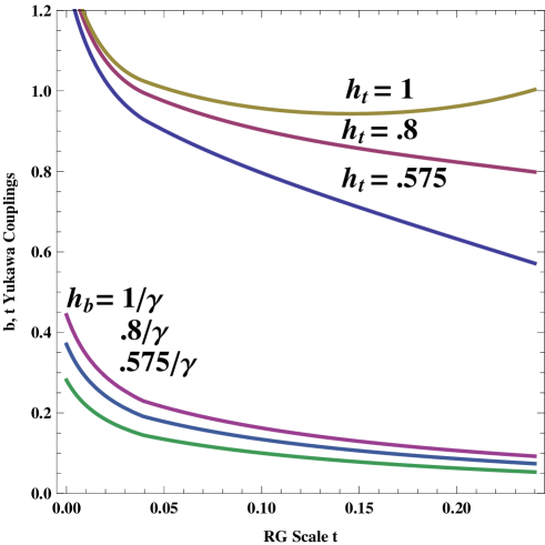
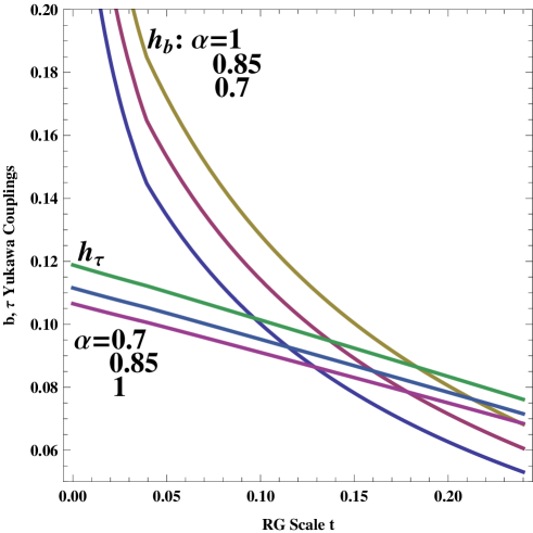
Figure 1: Left panel: The RG evolution of the Yukawa coupling $h_{b}(Q)$ for the bottom quark and $h_{\tau}(Q)$ for the $\tau$ lepton for $\alpha=1,0.85,0.7$ (see Table (2)) from the grand unification scale to the electroweak scale where t labeling the x-axis is defined so that $t=ln(Q({\rm GeV})/16\pi^{2}$. For the analysis of the figure in the left panel we have chosen $h_{t}(M_{G})=0.575$ and $h_{b}(M_{G})$ and $h_{\tau}(M_{G})$ are then determined from Table (2). Right panel: The RG evolution of the Yukawa coupling $h_{b}(M_{G})$ and of $h_{t}(M_{G})$ for values of $h_{t}(M_{G})=1,.8,.575$ and for $h_{b}(M_{G})=1/\gamma,.8/\gamma,.575/\gamma$ for the case $\alpha=.7$ from the grand unification scale to the electroweak scale where $\gamma=10.73$ as given in Table (2). The convergence of the top Yukawa couplings at low scales is due to the presence of the Landau pole for the top Yukawa coupling. The best fit to the $b,\tau,t$ masses given in Eq.(88) occurs for $\alpha=.7$, $h_{t}(M_{G})=0.575$.

Next we look at the ratio $m_{t}/m_{b}$, which we write in the following form

$$\frac{m_{t}}{m_{b}}=\frac{h_{t}}{h_{b}}\tan\beta,\leavevmode\nobreak\ \leavevmode\nobreak\ \tan\beta=\frac{<{\bf{Q}}^{5}>}{<{\bf{P}}_{5}>}.$$ (84)

Our analysis using Eq.(67) and Eq.(79) gives for $\gamma=h_{t}/h_{b}$ at the GUT scale the result

$$\gamma=\frac{h_{t}}{h_{b}}=\frac{160}{3}\frac{f_{33}^{(120}}{f_{33}^{(45)}}\frac{y_{45}}{y_{120}}\sqrt{\frac{1+\frac{3}{32}y_{120}^{2}}{64+6\left(\frac{y_{120}}{y_{45}}\right)^{2}+\frac{3}{8}y_{120}^{2}}}.$$ (85)

Since the values of $y_{45}$ and $y_{120}$ are constrained by Eq.(83), we solve Eqs.(83) and (85) to determine the values of $h_{t}/h_{b}$ at the GUT scale as a function of $\alpha$. These results are exhibited in Table(2).

Table 2: Values of $\displaystyle{{h_{{{t}}}}}/{{h_{{{b}}}}}$ vs $\displaystyle{{h_{{{b}}}}}/{{h_{{{\tau}}}}}$ at $Q=M_{G}$
$\alpha=h_{b}(M_{G})/h_{\tau}(M_{G})$	.7	.75	.8	.85	.9	.95	1
$\gamma=h_{t}(M_{G})/h_{b}(M_{G})$	10.73	10.22	9.76	9.40	8.99	8.65	8.35

Eventually at low scales after the VEV formation, the Higgs doublets $({\bf{Q}}^{5},{\bf{P}}_{5})$ will develop VEVs and lead to mass generation for the top quark, for the bottom quark and for the tau lepton so that

$$m_{t}=\frac{h_{t}v\sin\beta}{\sqrt{2}},m_{b}=\frac{h_{b}v\cos\beta}{\sqrt{2}},m_{\tau}=\frac{h_{\tau}v\cos\beta}{\sqrt{2}},$$ (86)

where $v=\sqrt{<{\bf Q}^{5}>^{2}+<{\bf P}_{5}>^{2}}$ and where numerically $v=246$ GeV.

In a typical $SO(10)$ grand unification group where the electroweak symmetry is broken with a $10$ plet of Higgs, a $b-\tau-t$ unification typically requires a large $\tan\beta$, i.e., a value of $\tan\beta$ as large as 40-50[7]. However, from the analysis above we find that a $b-\tau-t$ unification can occur for much smaller values of $\tan\beta$ (this was also noted in [4]). As is conventionally done, we allow for the possibility of Planck scale type corrections, and do not assume a rigid equality of the bottom and tau Yukawa couplings[8, 9, 10]. Specifically we assume $h_{b}(M_{G})=\alpha h_{\tau}(M_{G})$ where $\alpha$ can deviate from unity. With a given choice of $\alpha$, the ratio $h_{t}/h_{b}$ is then determined. In Table (2) we list the allowed values of $h_{t}/h_{b}$ for $\alpha$ in the range $.7-1.0$. Using these boundary conditions we have carried out a one loop analysis of the coupled partial differential equations for the three Yukawa couplings $h_{\tau},h_{b},h_{t}$ and for the three gauge coupling constants $g_{3},g_{2},g_{1}$ corresponding to the three gauge groups $SU(3)_{C},SU(2)_{L},U(1)$ starting from the grand unification scale $M_{G}$ and moving down to the electroweak scale. In addition to the GUT boundary conditions on the Yukawa couplings $h_{b},h_{\tau},h_{t}$ given by Table (2), the assumed range of $h_{t}$ is taken so that $|h_{t}|\leq 1$. Further, we assume that we have the GUT boundary conditions on the gauge couplings so that $g_{3}(M_{G})=g_{2}(M_{G})=g_{1}(M_{G})=g_{G}\simeq 0.7$.

The details of our numerical computation to determine $b,\tau,t$ mass are as follows: First we do the RG analysis in the region between the GUT scale and some average weak SUSY scale $M_{S}$, i.e., $M_{S}\leq Q\leq M_{G}$ using the boundary conditions at the GUT scale as discussed above. Here we use the RG evolution equations valid for MSSM. Below the scale $M_{S}$ we use the RG evolution equations appropriate for the Standard Model with proper matching done at the scale $M_{S}$. Numerical results for the evolution of the $b,\tau$ Yukawa couplings $h_{b}(Q),h_{\tau}(Q)$ are plotted in the right panel of Fig.(1) and for $h_{b}(Q),h_{t}(Q)$ are plotted in the left panel of Fig.(1) as a function of the scale $t=lnQ/16\pi^{2}$. The rapid convergence of the yukawas couplings for the top at low scale is due to the well known Landau pole singularity in the top Yukawa coupling[8, 11]. In the RG analysis we compute the values of $m_{t}(m_{t})$ which is related to the pole mass $m_{t}^{p}$ by the relation

$$m_{t}^{p}=m_{t}(m_{t})[1+\frac{4}{3\pi}\alpha_{s}(m_{t})].$$ (87)

For the computation of $m_{b}(m_{b})$ we use three loop QCD and one loop EM evolution between the scale $M_{Z}$ and the scale $m_{b}$. The procedure of the analysis is as given in [8, 9]. Using the result of Table 1 for $h_{b}/h_{\tau}=.7$ we find a determination of $\tan\beta$ and the following fit to the $b,t$ pole masses using the $\tau$ lepton mass as an input $m_{\tau}=1.776$ GeV, so that

$$\tan\beta=8,\leavevmode\nobreak\ m_{b}=4.53\leavevmode\nobreak\ {\rm GeV},\leavevmode\nobreak\ m_{t}^{p}=172.9\leavevmode\nobreak\ {\rm GeV}.\leavevmode\nobreak\$$ (88)

The above are to be compared with the experimental data on the $b$ quark and on the top quark mass, i.e., $m_{b}=4.2^{+0.17}_{-0.07}$ GeV, $m_{t}=171.3\pm 1.1\pm 1.2$ GeV[12]. Thus our one loop analysis is within about 2$\sigma$ of the $b$ quark mass and within one sigma of the top quark mass. We note that for the model above $b-\tau-t$ unification is achieved for a value which is much smaller than what typically appears in $b-\tau-t$ unification analyses.

6 Tau Neutrino Mass

We begin by collecting all the relevant terms in the cubic Lagrangian that would contribute to neutrino mass:

$$\sum L=-2:\leavevmode\nobreak\ \leavevmode\nobreak\ \leavevmode\nobreak\ \leavevmode\nobreak\ {\mathsf{L}}_{1,{\nu_{\tau}}}^{(120)} = -\frac{16}{\sqrt{15}}f^{(120)}_{33}<{\bf Q}_{5}>{}^{(1_{16})}\!{{\overline{\mbox{\LARGE$\nu$}}}}_{R\tau}{}^{({{5}}_{120})}\!{\mbox{\LARGE$\nu$}}_{L\tau}^{\mathsf{c}}+\textnormal{H.c.},$$

$$\sum L=0:\leavevmode\nobreak\ \leavevmode\nobreak\ \leavevmode\nobreak\ \leavevmode\nobreak\ {\mathsf{L}}_{2,{\nu_{\tau}}}^{(120)} = 16\sqrt{3}f^{(120)}_{33}<{\bf Q}^{5}>{}^{(1_{16})}\!{{\overline{\mbox{\LARGE$\nu$}}}}_{R\tau}{}^{({\overline{5}}_{120})}\!{\mbox{\LARGE$\nu$}}_{L\tau}+\textnormal{H.c.},$$

$$\sum L=0:\leavevmode\nobreak\ \leavevmode\nobreak\ \leavevmode\nobreak\ \leavevmode\nobreak\ {\mathsf{L}}_{3,{\nu_{\tau}}}^{(120)} = 8\sqrt{3}f^{(120)}_{33}q\leavevmode\nobreak\ \leavevmode\nobreak\ {}^{(5_{120})}\!{{\overline{\mbox{\LARGE$\nu$}}}}_{R\tau}{}^{({\overline{5}}_{16})}\!{\mbox{\LARGE$\nu$}}_{L\tau}+\textnormal{H.c.},$$

$$\sum L=0:\leavevmode\nobreak\ \leavevmode\nobreak\ \leavevmode\nobreak\ \leavevmode\nobreak\ {\mathsf{L}}_{4,{\nu_{\tau}}}^{(120)} = 2m_{F}^{(120)}\leavevmode\nobreak\ \leavevmode\nobreak\ {}^{(5_{120})}\!{{\overline{\mbox{\LARGE$\nu$}}}}_{R\tau}{}^{({\overline{5}}_{120})}\!{\mbox{\LARGE$\nu$}}_{L\tau}+\textnormal{H.c.},$$

$$\sum L=-2:\leavevmode\nobreak\ \leavevmode\nobreak\ \leavevmode\nobreak\ \leavevmode\nobreak\ {\mathsf{L}}_{6,{\nu_{\tau}}}^{(45)} = m_{F}^{(45)}\leavevmode\nobreak\ \leavevmode\nobreak\ {}^{(1_{45})}\!{{\overline{\mbox{\LARGE$\nu$}}}}_{R\tau}{}^{({{1}}_{45})}\!{\mbox{\LARGE$\nu$}}_{L\tau}^{\mathsf{c}}+\textnormal{H.c.},$$

$$\sum L=-2:\leavevmode\nobreak\ \leavevmode\nobreak\ \leavevmode\nobreak\ \leavevmode\nobreak\ {\mathsf{L}}_{{\rm quartic},{\nu_{\tau}}} = m_{F}^{(16)}\leavevmode\nobreak\ \leavevmode\nobreak\ {}^{(1_{16})}\!{{\overline{\mbox{\LARGE$\nu$}}}}_{R\tau}{}^{({{1}}_{16})}\!{\mbox{\LARGE$\nu$}}_{L\tau}^{\mathsf{c}}+\textnormal{H.c.},$$ (89)

where we have identified lepton number ($L$) conserving (Dirac-like) and lepton number violating violating (Majorana-like) interactions. There are no couplings of the $1_{45}$ state with the other neutrino states , and thus the $1_{45}$ which is superheavy can be integrated out and does not enter into the rest of the analysis. Further, the states $5_{120}$ and $\bar{5}_{120}$ are also superheavy and can be eliminated leaving an effective Dirac mass term involving $1_{16}$ and $\bar{5}_{16}$ and a Majorana mass term for the $1_{16}$ which is the last term in Eq.(6). These remaining interactions then produce a Type I See Saw mass for the light tau neutrino which is given by

$$m_{\nu_{\tau}}\simeq\frac{m_{D}^{2}\sin^{2}\beta}{m_{F}^{(16)}},\leavevmode\nobreak\ \leavevmode\nobreak\ m_{D}\simeq 96(f_{33}^{(120)})^{2}v\left(\frac{q}{m_{F}^{(120)}}\right)$$ (90)

It is interesting to note the dependence of the neutrino mass on $\sin\beta$ in Eq.(90) which reflects the chose connection of the neutrino mass with electroweak physics. Now the choice $f_{33}^{(120)}\sim.2$, $q/M_{F}^{(120}\sim 1$ and $M_{F}^{(16)}=10^{16}$ GeV, and $v=246$ GeV, $\sin\beta\sim 1$ leads to a Type I See Saw mass of $m_{\nu_{\tau}}\simeq 0.1eV$. A more complete analysis of fermion masses including also the Type II and Type III See Saw masses in the unified Higgs framework will be given elsewhere[13].

7 Proton stability

Grand unified models of particle interactions typically lead to higgsino mediated proton decay via baryon and lepton ($B\&L$) number violating dimension five operators. There are severe restrictions on the size of such operators from the current limits on proton decay[2] (For some recent works on proton decay see[14, 15] and for a recent review of experiment see [16]). In the present context such $B\&L$ violating dimension five operators arise from the quartic interactions of the type $16\cdot 16\cdot 144\cdot 144$ and $16\cdot 16\cdot\overline{144}\cdot\overline{144}$ operators. In addition there are $B\&L$ violating dimension five operators from the $16\cdot 120\cdot 144$ and from $16\cdot 45\cdot\overline{144}$. In Ref.[15] a cancelation mechanism to suppress proton decay was advocated and some specific examples of such a cancelation were also exhibited there. Such a cancelation mechanism could also work for dimension five operators arising from the above mentioned interactions. An analysis of proton lifetime within the unified Higgs framework without invoking the cancellation mechanism is given in a recent work[17] where the decay lifetime $\tau(p\to\bar{\nu}K^{+})$ is found to lie in the range $(1.4\times 10^{35}-1.9\times 10^{33})$yr for $\tan\beta$ in the range $\tan\beta=2-20$. This puts the proton lifetime in the unified Higgs model at the edge of detection in improved proton decay experiment[16, 22].

8 Conclusion

In this work we have carried out an analysis of the Yukawa couplings that arise from quartic couplings of the type $\frac{1}{\Lambda}16\cdot 16\cdot 144\cdot 144$ which can contribute to the quark-charged lepton and neutrino masses. Such Yukawas arise after spontaneous breaking of the $SO(10)$ gauge symmetry at the grand unification scale where the $144$ and $\overline{144}$ of the Higgs multiplets develop vacuum expectation values. Computations of these Yukawa couplings are non-trivial involving special techniques which are utilized for their computation in this work. Thus after the $144$ of the Higgs fields develop superheavy VEVs, the interaction $\frac{1}{\Lambda}16\cdot 16\cdot 144\cdot 144$ generates Yukawa couplings for the quarks, charged leptons and the neutrinos which we calculate. These Yukawas are typically $O(\frac{<144>}{\Lambda})\sim O(\frac{M_{G}}{M_{St}})$ and thus typically of size $10^{-2}$. These Yukawa couplings are thus appropriate for the analysis of the mass matrices for the first and second generation masses. However, these Yukawas are too small for the generation of third generation fermion masses. To allow for significantly larger third generation fermion masses we considered cubic couplings involving $45$ and $120$ plets of matter fields, i.e., couplings of the type $16\cdot 45\cdot\overline{144}$ and $16\cdot 120\cdot 144$. These interactions lead to cubic couplings of size appropriate for the third generation. An analysis for the quarks, charged lepton and neutrino masses was also given. It is shown that the $144$ plet Higgs couplings allow for a See Saw mechanism for the generation of neutrino masses. The analysis of the Yukawa interactions given here would be of significant value in the further development of the $SO(10)$ phenomenology in the unified Higgs framework.

Acknowledgements: We thank K.S. Babu and Ilia Gogoladze for discussions. This work was supported in part by NSF grant PHY-0757959.

Table 1: Fermion mass parameters from quartic couplings
$A^{(10)}_{1\leavevmode\nobreak\ \acute{a}\acute{b}}$	$-48\zeta_{\acute{a}\acute{b},\acute{c}\acute{d}}^{{}^{(10)(+)}}q_{\acute{c}}<{{\bf Q}}_{{\acute{d}}}^{5}>$	$A^{(10)}_{2\leavevmode\nobreak\ \acute{a}\acute{b}}$	$\frac{24}{\sqrt{5}}\xi_{\acute{a}\acute{b},\acute{c}\acute{d}}^{{}^{(10)(+)}}p_{\acute{c}}<{{\bf P}}_{{\acute{d}}}^{\prime 5}>\cos\vartheta_{\mathsf{D}}$
$A^{(10)}_{3\leavevmode\nobreak\ \acute{a}\acute{b}}$	$\frac{24}{\sqrt{5}}\xi_{\acute{a}\acute{b},\acute{c}\acute{d}}^{{}^{(10)(+)}}p_{\acute{c}}<{\widetilde{\bf P}}_{{\acute{d}}}^{\prime 5}>\sin\vartheta_{\mathsf{D}}$	$A^{(10)}_{4\leavevmode\nobreak\ \acute{a}\acute{b}}$	$-40\sqrt{3}\xi_{\acute{a}\acute{b},\acute{c}\acute{d}}^{{}^{(10)(+)}}p_{\acute{c}}<{{\bf P}}_{{\acute{d}}}^{\prime 5}>\sin\vartheta_{\mathsf{D}}$
$A^{(10)}_{5\leavevmode\nobreak\ \acute{a}\acute{b}}$	$40\sqrt{3}\xi_{\acute{a}\acute{b},\acute{c}\acute{d}}^{{}^{(10)(+)}}p_{{\acute{c}}}<{\widetilde{\bf P}}_{{\acute{d}}}^{\prime 5}>\cos\vartheta_{\mathsf{D}}$	$A^{(10)}_{6\leavevmode\nobreak\ \acute{a}\acute{b}}$	$6\lambda_{\acute{a}\acute{d},\acute{b}\acute{c}}^{{}^{(10)}}q_{\acute{c}}<{{\bf Q}}_{{\acute{d}}}^{5}>$
$A^{(45)}_{1\leavevmode\nobreak\ \acute{a}\acute{b}}$	$-\frac{2}{\sqrt{5}}(4\lambda_{{\acute{a}}{\acute{c}},{\acute{b}}{\acute{d}}}^{{}^{(45)}}-5\lambda_{{\acute{a}}{\acute{d}},{\acute{b}}{\acute{c}}}^{{}^{(45)}})p_{\acute{c}}<{\bf{P}}_{\acute{d}}^{\prime 5}>\cos\vartheta_{\mathsf{D}}$	$A^{(45)}_{2\leavevmode\nobreak\ \acute{a}\acute{b}}$	$-\frac{2}{\sqrt{5}}(4\lambda_{{\acute{a}}{\acute{c}},{\acute{b}}{\acute{d}}}^{{}^{(45)}}-5\lambda_{{\acute{a}}{\acute{d}},{\acute{b}}{\acute{c}}}^{{}^{(45)}})p_{\acute{c}}<{\widetilde{\bf{P}}}_{\acute{d}}^{\prime 5}>\sin\vartheta_{\mathsf{D}}$
$A^{(45)}_{3\leavevmode\nobreak\ \acute{a}\acute{b}}$	$\frac{2}{\sqrt{3}}(2\lambda_{{\acute{a}}{\acute{c}},{\acute{b}}{\acute{d}}}^{{}^{(45)}}-9\lambda_{{\acute{a}}{\acute{d}},{\acute{b}}{\acute{c}}}^{{}^{(45)}})p_{\acute{c}}<{{\bf{P}}}_{\acute{d}}^{\prime 5}>\sin\vartheta_{\mathsf{D}}$	$A^{(45)}_{4\leavevmode\nobreak\ \acute{a}\acute{b}}$	$-\frac{2}{\sqrt{3}}(2\lambda_{{\acute{a}}{\acute{c}},{\acute{b}}{\acute{d}}}^{{}^{(45)}}-9\lambda_{{\acute{a}}{\acute{d}},{\acute{b}}{\acute{c}}}^{{}^{(45)}})p_{\acute{c}}<{\widetilde{\bf{P}}}_{\acute{d}}^{\prime 5}>\cos\vartheta_{\mathsf{D}}$
$A^{(54)}_{1\leavevmode\nobreak\ \acute{a}\acute{b}}$	$-\frac{4}{\sqrt{3}}\lambda_{{\acute{a}}{\acute{c}},{\acute{b}}{\acute{d}}}^{{}^{(54)}}p_{\acute{c}}<{{\bf{P}}}_{\acute{d}}^{\prime 5}>\sin\vartheta_{\mathsf{D}}$	$A^{(54)}_{2\leavevmode\nobreak\ \acute{a}\acute{b}}$	$\frac{4}{\sqrt{3}}\lambda_{{\acute{a}}{\acute{c}},{\acute{b}}{\acute{d}}}^{{}^{(54)}}p_{\acute{c}}<{\widetilde{\bf{P}}}_{\acute{d}}^{\prime 5}>\cos\vartheta_{\mathsf{D}}$
$A^{(54)}_{3\leavevmode\nobreak\ \acute{a}\acute{b}}$	$\frac{3}{\sqrt{5}}\lambda_{{\acute{a}}{\acute{c}},{\acute{b}}{\acute{d}}}^{{}^{(54)}}p_{\acute{c}}<{{\bf{P}}}_{\acute{d}}^{\prime 5}>\cos\vartheta_{\mathsf{D}}$	$A^{(54)}_{4\leavevmode\nobreak\ \acute{a}\acute{b}}$	$\frac{3}{\sqrt{5}}\lambda_{{\acute{a}}{\acute{c}},{\acute{b}}{\acute{d}}}^{{}^{(54)}}p_{\acute{c}}<{\widetilde{\bf{P}}}_{\acute{d}}^{\prime 5}>\sin\vartheta_{\mathsf{D}}$
$A^{(126)}_{\leavevmode\nobreak\ \acute{a}\acute{b}}$	$-\frac{32}{5}\varrho_{\acute{a}\acute{b},\acute{c}\acute{d}}^{{}^{(126,\overline{126})(+)}}q_{\acute{c}}<{{\bf Q}}_{{\acute{d}}}^{5}>$
$B^{(10)}_{1\leavevmode\nobreak\ \acute{a}\acute{b}}$	$\frac{24}{\sqrt{5}}\zeta_{\acute{a}\acute{b},\acute{c}\acute{d}}^{{}^{(10)(+)}}q_{\acute{c}}<{\bf{Q}}_{\acute{d}5}^{\prime}>\cos\vartheta_{\mathsf{D}}$	$B^{(10)}_{2\leavevmode\nobreak\ \acute{a}\acute{b}}$	$\frac{24}{\sqrt{5}}\zeta_{\acute{a}\acute{b},\acute{c}\acute{d}}^{{}^{(10)(+)}}q_{\acute{c}}<{\widetilde{\bf{Q}}}_{\acute{d}5}^{\prime}>\sin\vartheta_{\mathsf{D}}$
$B^{(10)}_{3\leavevmode\nobreak\ \acute{a}\acute{b}}$	$-40\sqrt{3}\zeta_{\acute{a}\acute{b},\acute{c}\acute{d}}^{{}^{(10)(+)}}q_{\acute{c}}<{\bf{Q}}_{\acute{d}5}^{\prime}>\sin\vartheta_{\mathsf{D}}$	$B^{(10)}_{4\leavevmode\nobreak\ \acute{a}\acute{b}}$	$40\sqrt{3}\zeta_{\acute{a}\acute{b},\acute{c}\acute{d}}^{{}^{(10)(+)}}q_{\acute{c}}<{\widetilde{\bf{Q}}}_{\acute{d}5}^{\prime}>\cos\vartheta_{\mathsf{D}}$
$B^{(10)}_{5\leavevmode\nobreak\ \acute{a}\acute{b}}$	$48\xi_{\acute{a}\acute{b},\acute{c}\acute{d}}^{{}^{(10)(+)}}p_{\acute{c}}<{\bf{P}}_{\acute{d}5}>$	$B^{(10)}_{6\leavevmode\nobreak\ \acute{a}\acute{b}}$	$-\frac{2}{\sqrt{5}}\lambda_{\acute{a}\acute{c},\acute{b}\acute{d}}^{{}^{(10)}}q_{\acute{c}}<{\bf{Q}}_{\acute{d}5}^{\prime}>\cos\vartheta_{\mathsf{D}}$
$B^{(10)}_{7\leavevmode\nobreak\ \acute{a}\acute{b}}$	$-\frac{2}{\sqrt{5}}\lambda_{\acute{a}\acute{c},\acute{b}\acute{d}}^{{}^{(10)}}q_{\acute{c}}<{\widetilde{\bf{Q}}}_{\acute{d}5}^{\prime}>\sin\vartheta_{\mathsf{D}}$	$B^{(45)}_{\leavevmode\nobreak\ \acute{a}\acute{b}}$	$-2\lambda_{\acute{a}\acute{d},\acute{b}\acute{c}}^{{}^{(45)}}p_{\acute{c}}<{\bf{P}}_{\acute{d}5}>$
$B^{(54)}_{\leavevmode\nobreak\ \acute{a}\acute{b}}$	$-10\lambda_{\acute{a}\acute{d},\acute{b}\acute{c}}^{{}^{(54)}}p_{\acute{c}}<{\bf{P}}_{\acute{d}5}>$	$B^{(126)}_{1\leavevmode\nobreak\ \acute{a}\acute{b}}$	$\frac{11}{15\sqrt{5}}\varrho_{\acute{a}\acute{b},\acute{c}\acute{d}}^{{}^{(126,\overline{126})(+)}}q_{\acute{c}}<{{\bf Q}}_{{\acute{d}}5}^{\prime}>\cos\vartheta_{\mathsf{D}}$
$B^{(126)}_{2\leavevmode\nobreak\ \acute{a}\acute{b}}$	$\frac{11}{15\sqrt{5}}\varrho_{\acute{a}\acute{b},\acute{c}\acute{d}}^{{}^{(126,\overline{126})(+)}}q_{\acute{c}}<{\widetilde{\bf{Q}}}_{\acute{d}5}^{\prime}>\sin\vartheta_{\mathsf{D}}$	$B^{(126)}_{3\leavevmode\nobreak\ \acute{a}\acute{b}}$	$-\frac{7}{15\sqrt{3}}\varrho_{\acute{a}\acute{b},\acute{c}\acute{d}}^{{}^{(126,\overline{126})(+)}}q_{\acute{c}}<{{\bf Q}}_{{\acute{d}}5}^{\prime}>\sin\vartheta_{\mathsf{D}}$
$B^{(126)}_{4\leavevmode\nobreak\ \acute{a}\acute{b}}$	$\frac{7}{15\sqrt{3}}\varrho_{\acute{a}\acute{b},\acute{c}\acute{d}}^{{}^{(126,\overline{126})(+)}}q_{\acute{c}}<{\widetilde{\bf{Q}}}_{\acute{d}5}^{\prime}>\cos\vartheta_{\mathsf{D}}$
$C^{(45)}_{\leavevmode\nobreak\ \acute{a}\acute{b}}$	$30\lambda_{\acute{a}\acute{c},\acute{b}\acute{d}}^{{}^{(45)}}p_{\acute{c}}p_{\acute{d}}$	$C^{(54)}_{\leavevmode\nobreak\ \acute{a}\acute{b}}$	$-30\lambda_{\acute{a}\acute{c},\acute{b}\acute{d}}^{{}^{(54)}}p_{\acute{c}}p_{\acute{d}}$
$C^{(10)}_{1\leavevmode\nobreak\ \acute{a}\acute{b}}$	$-\frac{4}{\sqrt{5}}\lambda_{\acute{a}\acute{c},\acute{b}\acute{d}}^{{}^{(10)}}<{{\bf Q}}_{{\acute{c}}}^{5}><{{\bf Q}}_{{\acute{d}5}}^{\prime}>\cos\vartheta_{\mathsf{D}}$	$C^{(10)}_{2\leavevmode\nobreak\ \acute{a}\acute{b}}$	$-\frac{4}{\sqrt{5}}\lambda_{\acute{a}\acute{c},\acute{b}\acute{d}}^{{}^{(10)}}<{{\bf Q}}_{{\acute{c}}}^{5}><{\widetilde{\bf Q}}_{{\acute{d}5}}^{\prime}>\sin\vartheta_{\mathsf{D}}$
$C^{(126)}_{1\leavevmode\nobreak\ \acute{a}\acute{b}}$	$-\frac{16}{15\sqrt{5}}\varrho_{\acute{a}\acute{b},\acute{c}\acute{d}}^{{}^{(126,\overline{126})(+)}}<{{\bf Q}}_{{\acute{c}}}^{5}><{{\bf Q}}_{{\acute{d}5}}^{\prime}>\cos\vartheta_{\mathsf{D}}$	$C^{(126)}_{2\leavevmode\nobreak\ \acute{a}\acute{b}}$	$-\frac{16}{15\sqrt{5}}\varrho_{\acute{a}\acute{b},\acute{c}\acute{d}}^{{}^{(126,\overline{126})(+)}}<{{\bf Q}}_{{\acute{c}}}^{5}><{\widetilde{\bf Q}}_{{\acute{d}5}}^{\prime}>\sin\vartheta_{\mathsf{D}}$
$D^{(45)}_{1\leavevmode\nobreak\ \acute{a}\acute{b}}$	$-\frac{1}{4}(\lambda_{{\acute{a}}{\acute{c}},{\acute{b}}{\acute{d}}}^{{}^{(45)}}-5\lambda_{{\acute{a}}{\acute{d}},{\acute{b}}{\acute{c}}}^{{}^{(45)}})<{\bf{P}}_{\acute{c}}^{\prime 5}><{\bf{P}}_{\acute{d}}^{\prime 5}>\cos^{2}\vartheta_{\mathsf{D}}$	$D^{(45)}_{2\leavevmode\nobreak\ \acute{a}\acute{b}}$	$-\frac{1}{4}(\lambda_{{\acute{a}}{\acute{c}},{\acute{b}}{\acute{d}}}^{{}^{(45)}}-5\lambda_{{\acute{a}}{\acute{d}},{\acute{b}}{\acute{c}}}^{{}^{(45)}})<{\widetilde{\bf{P}}}_{\acute{c}}^{\prime 5}><{\widetilde{\bf{P}}}_{\acute{d}}^{\prime 5}>\sin^{2}\vartheta_{\mathsf{D}}$
$D^{(45)}_{3\leavevmode\nobreak\ \acute{a}\acute{b}}$	$(\lambda_{{\acute{a}}{\acute{c}},{\acute{b}}{\acute{d}}}^{{}^{(45)}}+\lambda_{{\acute{a}}{\acute{d}},{\acute{b}}{\acute{c}}}^{{}^{(45)}})<{{\bf{P}}}_{\acute{c}}^{\prime 5}><{\widetilde{\bf{P}}}_{\acute{d}}^{\prime 5}>\cos\vartheta_{\mathsf{D}}\sin\vartheta_{\mathsf{D}}$	$D^{(54)}_{1\leavevmode\nobreak\ \acute{a}\acute{b}}$	$\frac{3}{80}(67\lambda_{{\acute{a}}{\acute{c}},{\acute{b}}{\acute{d}}}^{{}^{(54)}}-15\lambda_{{\acute{a}}{\acute{d}},{\acute{b}}{\acute{c}}}^{{}^{(54)}})<{\bf{P}}_{\acute{c}}^{\prime 5}><{\bf{P}}_{\acute{d}}^{\prime 5}>\cos^{2}\vartheta_{\mathsf{D}}$
$D^{(54)}_{2\leavevmode\nobreak\ \acute{a}\acute{b}}$	$\frac{3}{80}(67\lambda_{{\acute{a}}{\acute{c}},{\acute{b}}{\acute{d}}}^{{}^{(54)}}-15\lambda_{{\acute{a}}{\acute{d}},{\acute{b}}{\acute{c}}}^{{}^{(54)}})<{\widetilde{\bf{P}}}_{\acute{c}}^{\prime 5}><{\widetilde{\bf{P}}}_{\acute{d}}^{\prime 5}>\sin^{2}\vartheta_{\mathsf{D}}$	$D^{(54)}_{3\leavevmode\nobreak\ \acute{a}\acute{b}}$	$\frac{39}{20}(\lambda_{{\acute{a}}{\acute{c}},{\acute{b}}{\acute{d}}}^{{}^{(54)}}+\lambda_{{\acute{a}}{\acute{d}},{\acute{b}}{\acute{c}}}^{{}^{(54)}})<{{\bf{P}}}_{\acute{c}}^{\prime 5}><{\widetilde{\bf{P}}}_{\acute{d}}^{\prime 5}>\cos\vartheta_{\mathsf{D}}\sin\vartheta_{\mathsf{D}}$

Table caption: Fermion mass parameters arising from the interactions of the $144+\overline{144}$ with the 16 plet of matter after spontaneous breaking at the electroweak scale. All the coupling constants such as $\zeta_{\acute{a}\acute{b},\acute{c}\acute{d}}$ are scaled by the inverse mass $\Lambda^{-1}$ (see Eq.(2)) which is implicit in the definition of these couplings.

9 Appendix A: Formalism and Calculational Techniques

In this appendix we give a brief discussion of the formalism and of the calculational techniques used in the analysis of this paper. In the analysis we need couplings of the 144-plet and $\overline{144}$ plets of Higgs which includes self couplings of the type $(144\cdot\overline{144})^{2}$, quartic couplings with matter fields of the type $(16\cdot 16)(144\cdot 144)$, $(16\cdot 16)(\overline{144}\cdot\overline{144})$, $(16\cdot 144)(16\cdot 144)$, $(16\cdot\overline{144})(16\cdot\overline{144}),$ and cubic couplings with the matter fields $16\cdot 120\cdot 144$ and $16\cdot 45\cdot\overline{144}$. In $SO(10)$ the $144,\overline{144}$ are constrained vector-spinors which are gotten from the vector spinor $160$ by imposition of a constraint which removes $16$ components. Thus the 144-dimensional vector spinor $|\Upsilon_{(\pm)\mu}>$ is defined by

$$\Gamma_{\mu}|\Upsilon_{(\pm)\mu}>=0,$$ (91)

where $\Gamma_{\mu}$ satisfy a rank-10 Clifford algebra

$$\{\Gamma_{\mu},\Gamma_{\nu}\}=2\delta_{\mu\nu},$$ (92)

and where $\mu,\nu$ are the $SO(10)$ indices and take on the values $1,..,10$. We introduce now the notation for the components in $144$ and $\overline{144}$ in an $SU(5)\times U(1)$ decomposition. For the $144$ we have

$$144=5({\bf{\widehat{Q}}}^{i})+\bar{5}({\bf{\widehat{Q}}}_{i})+10({\bf{\widehat{Q}}}^{ij})+15({\bf{\widehat{Q}}}_{(S)}^{ij})+24({\bf{\widehat{Q}}}^{i}_{j})+40({\bf{\widehat{Q}}}^{ijk}_{l})+\overline{45}({\bf{\widehat{Q}}}^{i}_{jk}),$$ (93)

where $i,j,k,..$ are the $SU(5)$ indices which take on the values $1,..,5$. Similarly for $\overline{144}$ we introduce the notation

$$\overline{144}=\bar{5}({\bf{\widehat{P}}}_{i})+5({\bf{\widehat{P}}}^{i})+\overline{10}({\bf{\widehat{P}}}_{ij})+\overline{15}({\bf{\widehat{P}}}^{(S)}_{ij})+24({\bf{\widehat{P}}}^{i}_{j})+\overline{40}({\bf{\widehat{P}}}^{l}_{ijk})+45({\bf{\widehat{P}}}^{ij}_{k}).$$ (94)

Note that fields with a hat, $\leavevmode\nobreak\ \widehat{}\leavevmode\nobreak\$ stand for chiral superfields, while the ones without a hat represents the charge scalar component of the corresponding superfield.

For convenience of computations we will use the oscillator expansion technique[18, 19, 20]. (For an alternative technique see, e.g., [21]). In the oscillator method one uses for an $SO(10)$ group a set of 5 operators $b_{i},b_{i}^{\dagger}$ (i=1…5) which obey the anti-commutation relations

$$\{b_{i},b_{j}^{\dagger}\}=\delta_{ij},\leavevmode\nobreak\ \leavevmode\nobreak\ \{b_{i},b_{j}\}=0=\{b_{i}^{\dagger},b_{j}^{\dagger}\},$$ (95)

and the set of $10$ operators $\Gamma_{\mu}$ defined by

$$\Gamma_{2i}=(b_{i}+b_{i}^{\dagger}),\leavevmode\nobreak\ \leavevmode\nobreak\ \Gamma_{2i-1}=-i(b_{i}-b_{i}^{\dagger}).$$ (96)

Further, in the oscillator expansion[18, 19] the $16(|\Psi_{(+)}>)$ and $\overline{16}(|\Psi_{(-)}>)$ have the form

$$|\Psi_{(+)}>=|0>{\bf\widehat{P}}+\frac{1}{2}b_{i}^{\dagger}b_{j}^{\dagger}|0>{\bf\widehat{P}}^{ij}+\frac{1}{24}\epsilon^{ijklm}b_{j}^{\dagger}b_{k}^{\dagger}b_{l}^{\dagger}b_{m}^{\dagger}|0>{\bf P}_{i},$$ (97)

$$|\Psi_{(-)}>=b_{1}^{\dagger}b_{2}^{\dagger}b_{3}^{\dagger}b_{4}^{\dagger}b_{5}^{\dagger}|0>{\bf\widehat{Q}}+\frac{1}{12}\epsilon^{ijklm}b_{k}^{\dagger}b_{l}^{\dagger}b_{m}^{\dagger}|0>{\bf\widehat{Q}}_{ij}+b_{i}^{\dagger}|0>{\bf\widehat{Q}}^{i}.$$ (98)

The 160 plet spinor ($|\Psi_{(+)\mu}>$) and the $\overline{160}$ plet spinor ($|\Psi_{(-)\mu}>$) are defined by[3]

$$|\Psi_{(+)\acute{a}\mu}>=|0>{\bf\widehat{P}}_{\acute{a}\mu}+\frac{1}{2}b_{i}^{\dagger}b_{j}^{\dagger}|0>{\bf\widehat{P}}_{\acute{a}\mu}^{ij}+\frac{1}{24}\epsilon^{ijklm}b_{j}^{\dagger}b_{k}^{\dagger}b_{l}^{\dagger}b_{m}^{\dagger}|0>{\bf\widehat{P}}_{\acute{a}i\mu},$$ (99)

$$|\Psi_{(-)\acute{b}\mu}>=b_{1}^{\dagger}b_{2}^{\dagger}b_{3}^{\dagger}b_{4}^{\dagger}b_{5}^{\dagger}|0>{\bf\widehat{Q}}_{\acute{b}\mu}+\frac{1}{12}\epsilon^{ijklm}b_{k}^{\dagger}b_{l}^{\dagger}b_{m}^{\dagger}|0>{\bf\widehat{Q}}_{\acute{b}ij\mu}+b_{i}^{\dagger}|0>{\bf\widehat{Q}}_{\acute{b}\mu}^{i}.$$ (100)

The $144$ and $\overline{144}$ spinors $|\Upsilon_{(\pm)\mu}>$ are created from $|\Psi_{(\pm)\mu}>$ by removing the $16$ components $\Gamma_{\mu}|\Psi_{(\pm)\mu}>$ from $|\Psi_{(\pm)\mu}>$.

10 Appendix B: Details of analysis of the quartic couplings

In this Appendix we give further details of the computation of the couplings that go in the analysis of Sec.(3). First we note that the interactions $(16\cdot 16)_{10}(144\cdot 144)_{10}$, $(16\cdot 16)_{10}(\overline{144}\cdot\overline{144})_{10}$, $(16\cdot 16)_{120}(144\cdot 144)_{120}$, $(16\cdot 16)_{120}(\overline{144}\cdot\overline{144})_{120}$, and $(16\cdot 16)_{\overline{126}}(144\cdot 144)_{126}$ have already been computed in [5]. For the case when there is only generation of the $144+\overline{144}$ of Higgs multiplets, the interactions $(16\cdot 16)_{120}(144\cdot 144)_{120}$ and $(16\cdot 16)_{120}(\overline{144}\cdot\overline{144})_{120}$ do not contribute. On the other hand, for the analysis of Sec.(3) we also need the interactions $(16\cdot 144)_{10}(16\cdot 144)_{10}$, $(16\cdot\overline{144})_{45}(16\cdot\overline{144})_{45}$, $(16\cdot\overline{144})_{54}(16\cdot\overline{144})_{54}$. An explicit computations of these has not been given before and so in this Appendix we give an analysis of these interactions. We now give the details of the analysis.

10.1 $\mathbf{(16\cdot 144)_{10}(16\cdot 144)_{10}}$ coupling

The dimension-5 operator of the form $(16\cdot 144)_{10}(16\cdot 144)_{10}$ arises from the following superpotential

$${\mathsf{W}}^{{}^{(10)^{\prime}}}=\frac{1}{2}\Phi_{\mu{\cal S}}{\cal M}^{{}^{(10)}}_{{\cal S}{\cal S}^{\prime}}\Phi_{\mu{\cal S}^{\prime}}+j_{{\acute{a}\acute{b}}}^{{}^{(10)}}<\Psi^{*}_{(+)\acute{a}}|B|\Upsilon_{(-)\acute{b}\mu}>k_{{}_{{S}}}^{{}^{(10)}}\Phi_{\mu{\cal S}}.$$ (101)

Elimination of the $10$ plet gives,

$${\mathsf{W}}_{dim-5}^{(10)}=-2\lambda_{\acute{a}\acute{b},\acute{c}\acute{d}}^{{}^{(10)}}<\Psi_{(+)\acute{a}}^{*}|B|\Upsilon_{(-)\acute{b}c_{i}}><\Psi_{(+)\acute{c}}^{*}|B|\Upsilon_{(-)\acute{d}\bar{c}_{i}}>,$$ (102)

where

$$\lambda_{\acute{a}\acute{b},\acute{c}\acute{d}}^{{}^{(10)}}=j_{\acute{a}\acute{b}}^{{}^{(10)}}j_{\acute{c}\acute{d}}^{{}^{(10)}}k_{{}_{{\cal S}}}^{{}^{(10)}}\left[\widetilde{{\cal M}}^{{}^{(10)}}\left\{{\cal M}^{{}^{(54)}}\widetilde{{\cal M}}^{{}^{(10)}}-\bf{1}\right\}\right]_{{\cal S}{\cal S}^{\prime}}k_{{}_{{\cal S}^{\prime}}}^{{}^{(10)}},$$

$$\widetilde{{\cal M}}^{{}^{(10)}}=\left[{\cal M}^{{}^{(54)}}+\left({\cal M}^{{}^{(10)}}\right)^{\bf{T}}\right]^{-1}.$$ (103)

Mass terms in the last equation are given by

$${\mathsf{W}}^{{}^{(10)^{\prime}}}_{mass}=\lambda_{\acute{a}\acute{b},\acute{c}\acute{d}}^{{}^{(10)}}\left[-\frac{1}{\sqrt{5}}{\bf\widehat{M}}_{\acute{a}}^{ij\bf T}{{\bf\widehat{Q}}}_{\acute{b}j}{\bf\widehat{M}}_{\acute{c}k}^{\bf T}{{\bf\widehat{Q}}}_{\acute{d}i}^{k}+2{\bf\widehat{M}}_{\acute{a}i}^{\bf T}{{\bf\widehat{Q}}}_{\acute{b}}^{j}{\bf\widehat{M}}_{\acute{c}}^{\bf T}{{\bf\widehat{Q}}}_{\acute{d}j}^{i}+\frac{4}{\sqrt{5}}{\bf\widehat{M}}_{\acute{a}}^{\bf T}{{\bf\widehat{Q}}}_{\acute{b}}^{i}{\bf\widehat{M}}_{\acute{c}}^{\bf T}{{\bf\widehat{Q}}}_{\acute{d}i}\right].$$ (104)

10.2 $\mathbf{(16\cdot\overline{144})_{45}(16\cdot\overline{144})_{45}}$ coupling

To generate the $\mathbf{(16\cdot\overline{144})_{45}(16\cdot\overline{144})_{45}}$ coupling we consider the following superpotential

$${\mathsf{W}}^{{}^{(45)}}=\frac{1}{2}\Phi_{\mu\nu{\cal X}}{\cal M}^{{}^{(45)}}_{{\cal X}{\cal X}^{\prime}}\Phi_{\mu\nu{\cal X}^{\prime}}+\frac{1}{2!}h_{{\acute{a}\acute{b}}}^{{}^{(45)}}\Omega_{{\mu\nu,\acute{a}\acute{b}}}\Phi_{\mu\nu{\cal X}}k_{{}_{{\cal X}}}^{{}^{(45)}},$$ (105)

where $\Phi_{\mu\nu{\cal X}}$ is the $45$ plet field and

$$\Omega_{{\mu\nu,\acute{a}\acute{b}}}=<\Psi^{*}_{(+)\acute{a}}|B\Gamma_{\mu}|\Psi_{(+)\acute{b}\nu}>-<\Psi^{*}_{(+)\acute{a}}|B\Gamma_{\nu}|\Psi_{(+)\acute{b}\mu}>.$$ (106)

After elimination of the heavy $45$ of $SO(10)$ we get,

$${\mathsf{W}}^{{}^{(16\cdot{\overline{144}})_{45}(16\cdot{\overline{144}})_{45}}}=-\frac{1}{2}\lambda_{\acute{a}\acute{b},\acute{c}\acute{d}}^{{}^{(45)}}\Omega_{{\mu\nu,\acute{a}\acute{b}}}\Omega_{{\mu\nu,\acute{c}\acute{d}}}$$

$$=\lambda_{\acute{a}\acute{b},\acute{c}\acute{d}}^{{}^{(45)}}\left[-2<\Psi_{(+)\acute{a}}^{*}|Bb_{i}|\Psi_{(+)\acute{b}c_{j}}><\Psi_{(+)\acute{c}}^{*}|Bb_{i}^{\dagger}|\Psi_{(+)\acute{d}\bar{c}_{j}}>\right.$$

$$\left.+2<\Psi_{(+)\acute{a}}^{*}|Bb_{i}|\Psi_{(+)\acute{b}c_{j}}><\Psi_{(+)\acute{c}}^{*}|Bb_{j}^{\dagger}|\Psi_{(+)\acute{d}\bar{c}_{i}}>\right.$$

$$\left.-2<\Psi_{(+)\acute{a}}^{*}|Bb_{i}|\Psi_{(+)\acute{b}\bar{c}_{j}}><\Psi_{(+)\acute{c}}^{*}|Bb_{i}^{\dagger}|\Psi_{(+)\acute{d}c_{j}}>\right.$$

$$\left.+<\Psi_{(+)\acute{a}}^{*}|Bb_{i}|\Psi_{(+)\acute{b}\bar{c}_{j}}><\Psi_{(+)\acute{c}}^{*}|Bb_{j}|\Psi_{(+)\acute{d}\bar{c}_{i}}>\right.$$

$$\left.+<\Psi_{(+)\acute{a}}^{*}|Bb_{i}^{\dagger}|\Psi_{(+)\acute{b}c_{j}}><\Psi_{(+)\acute{c}}^{*}|Bb_{j}^{\dagger}|\Psi_{(+)\acute{d}c_{i}}>\right],$$ (107)

where we have defined

$$\lambda_{\acute{a}\acute{b},\acute{c}\acute{d}}^{{}^{(45)}}=h_{\acute{a}\acute{b}}^{{}^{(45)}}h_{\acute{c}\acute{d}}^{{}^{(45)}}k_{{}_{{\cal X}}}^{{}^{(45)}}\left[\widetilde{{\cal M}}^{{}^{(45)}}\left\{{\cal M}^{{}^{(45)}}\widetilde{{\cal M}}^{{}^{(45)}}-\bf{1}\right\}\right]_{{\cal X}{\cal X}^{\prime}}k_{{}_{{\cal X}^{\prime}}}^{{}^{(45)}},$$

$$\widetilde{{\cal M}}^{{}^{(45)}}=\left[{\cal M}^{{}^{(45)}}+\left({\cal M}^{{}^{(45)}}\right)^{\bf{T}}\right]^{-1}.$$ (108)

From the above we find the following couplings which contribute to the quark, lepton and neutrino masses[20]

$${\mathsf{W}}^{{}^{(45)}}_{mass}=\lambda_{\acute{a}\acute{b},\acute{c}\acute{d}}^{{}^{(45)}}\left[\epsilon_{ijklm}\left(-\frac{1}{\sqrt{5}}{\bf\widehat{M}}_{\acute{a}}^{ix\bf T}{{\bf\widehat{P}}}_{\acute{b}x}^{j}{\bf\widehat{M}}_{\acute{c}}^{kl\bf T}{{\bf\widehat{P}}}_{\acute{d}}^{m}+\frac{1}{2}{\bf\widehat{M}}_{\acute{a}}^{xy\bf T}{{\bf\widehat{P}}}_{\acute{b}y}^{i}{\bf\widehat{M}}_{\acute{c}}^{jk\bf T}{{\bf\widehat{P}}}_{\acute{d}x}^{lm}-\frac{1}{2}{\bf\widehat{M}}_{\acute{a}}^{ix\bf T}{{\bf\widehat{P}}}_{\acute{b}x}^{y}{\bf\widehat{M}}_{\acute{c}}^{jk\bf T}{{\bf\widehat{P}}}_{\acute{d}y}^{lm}\right)\right.$$

$$\left.+2{\bf\widehat{M}}_{\acute{a}}^{ij\bf T}\left({{\bf\widehat{P}}}_{\acute{b}j}^{k}{\bf\widehat{M}}_{\acute{c}i}^{\bf T}{{\bf\widehat{P}}}_{\acute{d}k}-{{\bf\widehat{P}}}_{\acute{b}j}^{k}{\bf\widehat{M}}_{\acute{c}k}^{\bf T}{{\bf\widehat{P}}}_{\acute{d}i}\right)\right.\left.+{\bf\widehat{M}}_{\acute{a}i}^{\bf T}\left(-\frac{3}{\sqrt{5}}{{\bf\widehat{P}}}_{\acute{b}}^{j}{\bf\widehat{M}}_{\acute{c}}^{\bf T}{{\bf\widehat{P}}}_{\acute{d}j}^{i}-2{{\bf\widehat{P}}}_{\acute{b}k}^{ij}{\bf\widehat{M}}_{\acute{c}}^{\bf T}{{\bf\widehat{P}}}_{\acute{dj}}^{k}\right)\right.$$

$$\left.-{\bf\widehat{M}}_{\acute{a}}^{\bf T}{{\bf\widehat{P}}}_{\acute{b}j}^{i}{\bf\widehat{M}}_{\acute{c}}^{\bf T}{{\bf\widehat{P}}}_{\acute{d}i}^{j}\right.\left.+{\bf\widehat{M}}_{\acute{a}i}^{\bf T}\left(-\frac{1}{4}{{\bf\widehat{P}}}_{\acute{b}}^{i}{\bf\widehat{M}}_{\acute{c}j}^{\bf T}{\widehat{\bf\widehat{P}}}_{\acute{d}}^{j}-\frac{5}{4}{{\bf\widehat{P}}}_{\acute{b}}^{j}{\bf\widehat{M}}_{\acute{c}j}^{\bf T}{\widehat{\bf\widehat{P}}}_{\acute{d}}^{i}\right)\right].$$ (109)

10.3 $\mathbf{(16\cdot\overline{144})_{54}(16\cdot\overline{144})_{54}}$ coupling

The 54-dimensional representation of $SO(10)$ is given by the tensor $\Phi_{\mu\nu}$ which is symmetric and traceless and is given by

$$\Delta_{{\mu\nu,\acute{a}\acute{b}}}=\Xi_{{\mu\nu,\acute{a}\acute{b}}}-\frac{1}{10}\delta_{\mu\nu}\Xi_{{\sigma\sigma,\acute{a}\acute{b}}},$$ (110)

where

$$\Xi_{{\mu\nu,\acute{a}\acute{b}}}=<\Psi^{*}_{(+)\acute{a}}|B\Gamma_{\mu}|\Psi_{(+)\acute{b}\nu}>+<\Psi^{*}_{(+)\acute{a}}|B\Gamma_{\nu}|\Psi_{(+)\acute{b}\mu}>.$$ (111)

To generate the desired coupling we consider the following superpotential

$${\mathsf{W}}^{{}^{(54)}}=\frac{1}{2}\Phi_{\mu\nu{\cal T}}{\cal M}^{{}^{(54)}}_{{\cal T}{\cal T}^{\prime}}\Phi_{\mu\nu{\cal T}^{\prime}}+\frac{1}{2!}h_{{\acute{a}\acute{b}}}^{{}^{(54)}}\Delta_{{\mu\nu,\acute{a}\acute{b}}}\Phi_{\mu\nu{\cal T}}k_{\cal T}^{{}^{(54)}}.$$ (112)

After elimination of the heavy $54$ of $SO(10)$ using the F-flatness conditions: $\frac{\partial{\mathsf{W}}^{(54)}}{\partial\Phi_{\mu\nu\cal{T}}}$ we get,

$${\mathsf{W}}_{dim-5}^{(54)}=-\frac{1}{2}\lambda_{\acute{a}\acute{b},\acute{c}\acute{d}}^{{}^{(45)}}\Delta_{{\mu\nu,\acute{a}\acute{b}}}\Delta_{{\mu\nu,\acute{c}\acute{d}}},$$ (113)

where we have defined

$$\lambda_{\acute{a}\acute{b},\acute{c}\acute{d}}^{{}^{(54)}}=h_{\acute{a}\acute{b}}^{{}^{(54)}}h_{\acute{c}\acute{d}}^{{}^{(54)}}k_{{}_{{\cal T}}}^{{}^{(54)}}\left[\widetilde{{\cal M}}^{{}^{(54)}}\left\{{\cal M}^{{}^{(54)}}\widetilde{{\cal M}}^{{}^{(54)}}-\bf{1}\right\}\right]_{{\cal T}{\cal T}^{\prime}}k_{{}_{{\cal T}^{\prime}}}^{{}^{(54)}},$$

$$\widetilde{{\cal M}}^{{}^{(54)}}=\left[{\cal M}^{{}^{(54)}}+\left({\cal M}^{{}^{(54)}}\right)^{\bf{T}}\right]^{-1}.$$ (114)

Using Eqs.(110) and (111) to expand Eq.(113), we obtain

$${\mathsf{W}}_{dim-5}^{(54)}=\lambda_{\acute{a}\acute{b},\acute{c}\acute{d}}^{{}^{(54)}}[-2<\Psi_{(+)\acute{a}}^{*}|Bb_{i}|\Upsilon_{(+)\acute{b}c_{j}}><\Psi_{(+)\acute{c}}^{*}|Bb_{i}^{\dagger}|\Upsilon_{(+)\acute{d}\bar{c}_{j}}>$$

$$-2<\Psi_{(+)\acute{a}}^{*}|Bb_{i}|\Upsilon_{(+)\acute{b}c_{j}}><\Psi_{(+)\acute{c}}^{*}|Bb_{j}^{\dagger}|\Upsilon_{(+)\acute{d}\bar{c}_{i}}>$$

$$-2<\Psi_{(+)\acute{a}}^{*}|Bb_{i}|\Upsilon_{(+)\acute{b}\bar{c}_{j}}><\Psi_{(+)\acute{c}}^{*}|Bb_{i}^{\dagger}|\Upsilon_{(+)\acute{d}c_{j}}>$$

$$-<\Psi_{(+)\acute{a}}^{*}|Bb_{i}|\Upsilon_{(+)\acute{b}\bar{c}_{j}}><\Psi_{(+)\acute{c}}^{*}|Bb_{j}|\Upsilon_{(+)\acute{d}\bar{c}_{i}}>$$

$$-<\Psi_{(+)\acute{a}}^{*}|Bb_{i}^{\dagger}|\Upsilon_{(+)\acute{b}c_{j}}><\Psi_{(+)\acute{c}}^{*}|Bb_{j}^{\dagger}|\Upsilon_{(+)\acute{d}c_{i}}>$$

$$+\frac{4}{5}<\Psi_{(+)\acute{a}}^{*}|Bb_{i}|\Upsilon_{(+)\acute{b}\bar{c}_{i}}><\Psi_{(+)\acute{c}}^{*}|Bb_{j}|\Upsilon_{(+)\acute{d}\bar{c}_{j}}>$$

$$+\frac{4}{5}<\Psi_{(+)\acute{a}}^{*}|Bb_{i}^{\dagger}|\Upsilon_{(+)\acute{b}c_{i}}><\Psi_{(+)\acute{c}}^{*}|Bb_{j}^{\dagger}|\Upsilon_{(+)\acute{d}c_{j}}>$$

$$+\frac{8}{5}<\Psi_{(+)\acute{a}}^{*}|Bb_{i}|\Upsilon_{(+)\acute{b}\bar{c}_{i}}><\Psi_{(+)\acute{c}}^{*}|Bb_{j}^{\dagger}|\Upsilon_{(+)\acute{d}c_{j}}>].$$ (115)

Finally, we look for the terms in the equation above which contribute to the quark, lepton and neutrino masses

$${\mathsf{W}}^{{}^{(54)}}_{mass}=\lambda_{\acute{a}\acute{b},\acute{c}\acute{d}}^{{}^{(54)}}\left[-\frac{1}{2}\epsilon_{ijklm}{\bf\widehat{M}}_{\acute{a}}^{xy\bf T}{{\bf\widehat{P}}}_{\acute{b}y}^{k}{\bf\widehat{M}}_{\acute{c}}^{ij\bf T}{{\bf\widehat{P}}}_{\acute{d}x}^{lm}-\frac{1}{2}\epsilon_{ijklm}{\bf\widehat{M}}_{\acute{a}}^{ix\bf T}{{\bf\widehat{P}}}_{\acute{b}x}^{y}{\bf\widehat{M}}_{\acute{c}}^{jk\bf T}{{\bf\widehat{P}}}_{\acute{d}y}^{lm}\right.$$

$$\left.-2{\bf\widehat{M}}_{\acute{a}}^{ij\bf T}{{\bf\widehat{P}}}_{\acute{b}i}^{k}{\bf\widehat{M}}_{\acute{c}j}^{\bf T}{{\bf\widehat{P}}}_{\acute{d}k}+2{\bf\widehat{M}}_{\acute{a}}^{ij\bf T}{{\bf\widehat{P}}}_{\acute{b}j}^{k}{\bf\widehat{M}}_{\acute{c}k}^{\bf T}{{\bf\widehat{P}}}_{\acute{d}i}+\frac{1}{\sqrt{5}}{\bf\widehat{M}}_{\acute{a}i}^{\bf T}{{\bf\widehat{P}}}_{\acute{b}}^{j}{\bf\widehat{M}}_{\acute{c}}^{\bf T}{{\bf\widehat{P}}}_{\acute{d}j}^{i}-2{\bf\widehat{M}}_{\acute{a}i}^{\bf T}{{\bf\widehat{P}}}_{\acute{b}k}^{ij}{\bf\widehat{M}}_{\acute{c}}^{\bf T}{{\bf\widehat{P}}}_{\acute{d}j}^{k}\right.$$

$$\left.+{\bf\widehat{M}}_{\acute{a}}^{\bf T}{{\bf\widehat{P}}}_{\acute{b}j}^{i}{\bf\widehat{M}}_{\acute{c}}^{\bf T}{{\bf\widehat{P}}}_{\acute{d}i}^{j}-\frac{201}{100}{\bf\widehat{M}}_{\acute{a}i}^{\bf T}{{\bf\widehat{P}}}_{\acute{b}}^{i}{\bf\widehat{M}}_{\acute{c}j}^{\bf T}{{\bf\widehat{P}}}_{\acute{d}}^{j}\right]+\frac{9}{20}\lambda_{\acute{a}\acute{d},\acute{c}\acute{b}}^{{}^{(54)}}{\bf\widehat{M}}_{\acute{a}i}^{\bf T}{{\bf\widehat{P}}}_{\acute{b}}^{i}{\bf\widehat{M}}_{\acute{c}j}^{\bf T}{{\bf\widehat{P}}}_{\acute{d}}^{j}.$$ (116)

11 Appendix C: General formulae on quark masses from quartic couplings

We give here the general formulae for the quark and lepton masses including all the relevant interactions. For the up quark we have

$$M^{u} = \sum_{i=1}^{5}A^{(10)}_{i}+\sum_{i=1}^{4}A^{(45)}_{i}+\sum_{i=1}^{2}A^{(54)}_{i}+A^{(126)}.$$ (117)

For the down type quarks and for the charged leptons we have

$$M^{d}_{\acute{a}\acute{b}} \equiv \left({X}+{Y}\right)_{\acute{a}\acute{b}},\leavevmode\nobreak\ \leavevmode\nobreak\ \leavevmode\nobreak\ \leavevmode\nobreak\ \leavevmode\nobreak\ M^{e}_{\acute{a}\acute{b}}\equiv\left({X}-3{Y}\right)_{\acute{a}\acute{b}},$$ (118)

$$X = \frac{1}{2}\sum_{i=1}^{5}B^{(10)}_{i}+\frac{9}{8}(B^{(10)}_{6}+B^{(10)}_{7})+\frac{3}{4}(-B^{(45)}+B^{(54)})$$ (119)

$$+\frac{21}{22}(B^{(126)}_{1}+B^{(126)}_{2})+\frac{3}{2}(B^{(126)}_{3}+B^{(126)}_{4}),$$

$$Y = \frac{1}{2}\sum_{i=1}^{5}B^{(10)}_{i}-\frac{1}{8}(B^{(10)}_{6}+B^{(10)}_{7})+\frac{7}{4}B^{(45)}+\frac{1}{4}B^{(54)}$$ (120)

$$+\frac{1}{22}(B^{(126)}_{1}+B^{(126)}_{2})-\frac{1}{2}(B^{(126)}_{3}+B^{(126)}_{4}).$$

For the Dirac neutrino we have

$$M^{D\nu} = \sum_{i=1}^{5}A^{(10)}_{i}+\frac{9}{8}\left[1-\frac{5}{4}\frac{\lambda_{{\acute{a}}{\acute{d}},{\acute{b}}{\acute{c}}}^{{}^{(45)}}}{\lambda_{{\acute{a}}{\acute{c}},{\acute{b}}{\acute{d}}}^{{}^{(45)}}}\right]^{-1}\left(A^{(45)}_{1}+A^{(45)}_{2}\right)+\frac{15}{4}\left[1-\frac{9}{2}\frac{\lambda_{{\acute{a}}{\acute{d}},{\acute{b}}{\acute{c}}}^{{}^{(45)}}}{{\lambda_{{\acute{a}}{\acute{c}},{\acute{b}}{\acute{d}}}^{{}^{(45)}}}}\right]^{-1}\left(A^{(45)}_{3}+A^{(45)}_{4}\right)$$ (121)

$$+\frac{15}{4}\left(A^{(54)}_{1}+A^{(54)}_{2}\right)+A^{(54)}_{3}+A^{(54)}_{4}-3A^{(126)},$$

$$M^{RR} = C^{(45)}+C^{(54)}+C^{(10)}_{1}+C^{(10)}_{2}+C^{(126)}_{1}+C^{(126)}_{2},$$

$$M^{LL} = \sum_{i=1}^{3}(D^{(45)}_{i}+D^{(54)}_{i}).$$ (122)

Subcases of these are discussed in Sec.(3.1).

12 Appendix D: Expansion of $\mathbf{(16\cdot 45\cdot\overline{144})}$ and $\mathbf{(16\cdot 120\cdot 144)}$ couplings

We give in this Appendix an $SU(5)\times U(1)$ expansion of $\mathbf{(16\cdot 45\cdot\overline{144})}$ and $\mathbf{(16\cdot 120\cdot 144)}$ couplings. Thus for the $\mathbf{(16\cdot 45\cdot\overline{144})}$ coupling we have the expansion

$${\mathsf{W}}^{16\cdot\cdot{45}\cdot\overline{144}} = 2h_{\acute{a}\acute{b}}^{(45)}\left\{<{\widehat{\Psi}}_{(+)\acute{a}}^{*}|Bb_{i}|{\widehat{\Upsilon}}_{(+)c_{j}}>\widehat{{\bf F}}_{\acute{b}ij}^{(45)}+<{\widehat{\Psi}}_{(+)\acute{a}}^{*}|Bb_{i}^{\dagger}|{\widehat{\Upsilon}}_{(+)\bar{c}_{j}}>\widehat{{\bf F}}_{\acute{b}}^{(45)ij}\right.$$

$$\left.+<{\widehat{\Psi}}_{(+)\acute{a}}^{*}|Bb_{i}^{\dagger}|{\widehat{\Upsilon}}_{(+)c_{j}}>\widehat{{\bf F}}_{\acute{b}j}^{(45)i}-<{\widehat{\Psi}}_{(+)\acute{a}}^{*}|Bb_{i}|{\widehat{\Upsilon}}_{(+)\bar{c}_{j}}>\widehat{{\bf F}}_{\acute{b}i}^{(45)j}\right.$$

$$\left.+\frac{1}{5}\left[<{\widehat{\Psi}}_{(+)\acute{a}}^{*}|Bb_{n}^{\dagger}|{\widehat{\Upsilon}}_{(+)c_{n}}>-<{\widehat{\Psi}}_{(+)\acute{a}}^{*}|Bb_{n}|{\widehat{\Upsilon}}_{(+)\bar{c}_{n}}>\right]\widehat{{\bf F}}_{\acute{b}}^{(45)}\right\},$$

$${\mathsf{W}}_{{{mass}}}^{(45)} = m_{F}^{(45)}\left[\widehat{{\bf F}}^{(45)ij}\widehat{{\bf F}}_{ij}^{(45)}-\widehat{{\bf F}}_{j}^{(45)i}\widehat{{\bf F}}_{i}^{(45)j}-\widehat{{\bf F}}^{(45)}\widehat{{\bf F}}^{(45)}\right].$$ (123)

and for the $\mathbf{(16\cdot 120\cdot 144)}$ couplings we have the expansion

$${\mathsf{W}}^{16\cdot{120}\cdot{144}} = h_{\acute{a}\acute{b}}^{(120)}\left\{4\epsilon_{ijklm}<{\widehat{\Psi}}_{(+)\acute{a}}^{*}|Bb_{i}b_{j}|{\widehat{\Upsilon}}_{(-)c_{k}}>\widehat{{\bf F}}_{\acute{b}}^{(120)lm}\right.$$

$$+ \negthinspace\negthinspace\negthinspace\left.4\epsilon^{ijklm}<{\widehat{\Psi}}_{(+)\acute{a}}^{*}|Bb_{i}^{\dagger}b_{j}^{\dagger}|{\widehat{\Upsilon}}_{(-)\bar{c}_{k}}>\widehat{{\bf F}}_{\acute{b}lm}^{(120)}\right.$$

$$+ \negthinspace\negthinspace\negthinspace\left.\left[4<{\widehat{\Psi}}_{(+)\acute{a}}^{*}|Bb_{i}b_{j}|{\widehat{\Upsilon}}_{(-)\bar{c}_{k}}>-8<{\widehat{\Psi}}_{(+)\acute{a}}^{*}|Bb_{k}^{\dagger}b_{j}|{\widehat{\Upsilon}}_{(-)c_{i}}>\right]\widehat{{\bf F}}_{\acute{b}ij}^{(120)k}\right.$$

$$+ \negthinspace\negthinspace\negthinspace\left.\left[4<{\widehat{\Psi}}_{(+)\acute{a}}^{*}|Bb_{i}^{\dagger}b_{j}^{\dagger}|{\widehat{\Upsilon}}_{(-)c_{k}}>-8<{\widehat{\Psi}}_{(+)\acute{a}}^{*}|Bb_{i}^{\dagger}b_{k}|{\widehat{\Upsilon}}_{(-)\bar{c}_{j}}>\right]\widehat{{\bf F}}_{\acute{b}k}^{(120)ij}\right.$$

$$+ \negthinspace\negthinspace\negthinspace\left.\left[-2<{\widehat{\Psi}}_{(+)\acute{a}}^{*}|Bb_{i}b_{n}|{\widehat{\Upsilon}}_{(-)\bar{c}_{n}}>-2<{\widehat{\Psi}}_{(+)\acute{a}}^{*}|Bb_{n}^{\dagger}b_{i}|{\widehat{\Upsilon}}_{(-)c_{n}}>+<{\widehat{\Psi}}_{(+)\acute{a}}^{*}|B\left(4+2b_{n}^{\dagger}b_{n}\right)|{\widehat{\Upsilon}}_{(-)c_{i}}>\right]\widehat{{\bf F}}_{\acute{b}i}^{(120)}\right.$$

$$+ \negthinspace\negthinspace\negthinspace\left.\left[2<{\widehat{\Psi}}_{(+)\acute{a}}^{*}|Bb_{n}^{\dagger}b_{i}^{\dagger}|{\widehat{\Upsilon}}_{(-)c_{n}}>+2<{\widehat{\Psi}}_{(+)\acute{a}}^{*}|Bb_{i}^{\dagger}b_{n}|{\widehat{\Upsilon}}_{(-)\bar{c}_{n}}>+<{\widehat{\Psi}}_{(+)\acute{a}}^{*}|B\left(4-2b_{n}^{\dagger}b_{n}\right)|{\widehat{\Upsilon}}_{(-)\bar{c}_{i}}>\right]\widehat{{\bf F}}_{\acute{b}}^{(120)i}\right\},$$

$${\mathsf{W}}_{{{mass}}}^{(120)} = m_{F}^{(120)}\left[\widehat{{\bf F}}^{(120)ij}\widehat{{\bf F}}_{ij}^{(120)}+\widehat{{\bf F}}_{ij}^{(120)k}\widehat{{\bf F}}_{k}^{(120)ij}+2\widehat{{\bf F}}^{(120)}_{i}\widehat{{\bf F}}^{(120)i}\right].$$ (124)

13 Appendix E: Contributions of ${\mathbf{16\cdot 45\cdot\overline{144}}}$ and ${\mathbf{16\cdot 120\cdot 144}}$ couplings to the ${\mathbf{b,\tau,t}}$ mass matrices

In this Appendix we give further details of the analysis of Sec.(4). Specifically we give here the terms that contribute to the mass matrices for the $b$ quark, for the $\tau$ lepton, and for the top quark that arise from the interactions of Eq.(20). We begin by listing the mass terms for the $b$ quark. We have

$${\mathsf{L}}_{2,{\textnormal{b}}}^{(45)} = -2\sqrt{2}f^{(45)}_{33}p\left[{}^{({\overline{10}}_{45})}\!\overline{{\Large{\textnormal{b}}}}_{{R}\alpha}\leavevmode\nobreak\ {}^{(10_{16})}\!{\Large{\textnormal{b}}}_{{L}}^{\alpha}\right]+\textnormal{H.c.},$$

$${\mathsf{L}}_{4,{\textnormal{b}}}^{(45)} = -2m_{F}^{(45)}\left[{}^{({\overline{10}}_{45})}\!\overline{{\Large{\textnormal{b}}}}_{{R}\alpha}\leavevmode\nobreak\ {}^{(10_{45})}\!{\Large{\textnormal{b}}}_{{L}}^{\alpha}\right]+\textnormal{H.c.},$$

$${\mathsf{L}}_{5,{\textnormal{b}}}^{(45)} = -2\sqrt{2}f^{(45)}_{33}<{\bf P}_{5}>\left[{}^{({\overline{5}}_{16})}\!\overline{{\Large{\textnormal{b}}}}_{{R}\alpha}\leavevmode\nobreak\ {}^{(10_{45})}\!{\Large{\textnormal{b}}}_{{L}}^{\alpha}\right]+\textnormal{H.c.},$$

$${\mathsf{L}}_{3,{\textnormal{b}}}^{(120)} = \frac{16}{\sqrt{3}}f^{(120)}_{33}q\left[{}^{({\overline{5}}_{16})}\!\overline{{\Large{\textnormal{b}}}}_{{R}\alpha}\leavevmode\nobreak\ {}^{(5_{120})}\!{\Large{\textnormal{b}}}_{{L}}^{\alpha}\right]+\textnormal{H.c.},$$

$${\mathsf{L}}_{4,{\textnormal{b}}}^{(120)} = -8\sqrt{\frac{3}{5}}f^{(120)}_{33}<{\bf Q}_{5}>\left[{}^{({\overline{5}}_{16})}\!\overline{{\Large{\textnormal{b}}}}_{{R}\alpha}\leavevmode\nobreak\ {}^{(10_{120})}\!{\Large{\textnormal{b}}}_{{L}}^{\alpha}\right]+\textnormal{H.c.},$$

$${\mathsf{L}}_{5,{\textnormal{b}}}^{(120)} = 8\sqrt{\frac{3}{5}}f^{(120)}_{33}<{\bf Q}_{5}>\left[{}^{({\overline{5}}_{120})}\!\overline{{\Large{\textnormal{b}}}}_{{R}\alpha}\leavevmode\nobreak\ {}^{(10_{16})}\!{\Large{\textnormal{b}}}_{{L}}^{\alpha}\right]+\textnormal{H.c.},$$

$${\mathsf{L}}_{6,{\textnormal{b}}}^{(120)} = \frac{16}{3}f^{(120)}_{33}<\widetilde{\bf Q}_{5}>\left[{}^{({\overline{5}}_{120})}\!\overline{{\Large{\textnormal{b}}}}_{{R}\alpha}\leavevmode\nobreak\ {}^{(10_{16})}\!{\Large{\textnormal{b}}}_{{L}}^{\alpha}\right]+\textnormal{H.c.},$$

$${\mathsf{L}}_{8,{\textnormal{b}}}^{(120)} = -\frac{16}{\sqrt{3}}f^{(120)}_{33}q\left[{}^{({\overline{10}}_{120})}\!\overline{{\Large{\textnormal{b}}}}_{{R}\alpha}\leavevmode\nobreak\ {}^{(10_{16})}\!{\Large{\textnormal{b}}}_{{L}}^{\alpha}\right]+\textnormal{H.c.},$$

$${\mathsf{L}}_{9,{\textnormal{b}}}^{(120)} = -2m_{F}^{(120)}\left[{}^{({\overline{10}}_{120})}\!\overline{{\Large{\textnormal{b}}}}_{{R}\alpha}\leavevmode\nobreak\ {}^{(10_{120})}\!{\Large{\textnormal{b}}}_{{L}}^{\alpha}\right]+\textnormal{H.c.},$$

$${\mathsf{L}}_{10,{\textnormal{b}}}^{(120)} = -2m_{F}^{(120)}\left[{}^{({\overline{5}}_{120})}\!\overline{{\Large{\textnormal{b}}}}_{{R}\alpha}\leavevmode\nobreak\ {}^{(5_{120})}\!{\Large{\textnormal{b}}}_{{L}}^{\alpha}\right]+\textnormal{H.c.}.$$ (125)

Next, we list the mass terms for the $\tau$ lepton. Here we have

$${\mathsf{L}}_{2,\mbox{\normalsize$\tau$}}^{(45)} = -12\sqrt{2}f^{(45)}_{33}p\left[\!{}^{(10_{16})}\overline{{\mbox{\LARGE$\tau$}}}_{{R}}\leavevmode\nobreak\ {}^{({\overline{10}}_{45})}\!{\mbox{\LARGE$\tau$}}_{{L}}\right]+\textnormal{H.c.},$$

$${\mathsf{L}}_{4,\mbox{\normalsize$\tau$}}^{(45)} = -2m_{F}^{(45)}\left[{}^{(10_{45})}\!\overline{{\mbox{\LARGE$\tau$}}}_{{R}}\leavevmode\nobreak\ {}^{({\overline{10}}_{45})}\!{\mbox{\LARGE$\tau$}}_{{L}}^{\alpha}\right]+\textnormal{H.c.},$$

$${\mathsf{L}}_{5,\mbox{\normalsize$\tau$}}^{(45)} = 2\sqrt{2}f^{(45)}_{33}<{\bf P}_{5}>\left[{}^{(10_{45})}\!\overline{{\mbox{\LARGE$\tau$}}}_{{R}}\leavevmode\nobreak\ {}^{({\overline{5}}_{16})}\!{\mbox{\LARGE$\tau$}}_{{L}}\right]+\textnormal{H.c.},$$

$${\mathsf{L}}_{3,\mbox{\normalsize$\tau$}}^{(120)} = -8\sqrt{3}f^{(120)}_{33}q\left[{}^{(5_{120})}\!\overline{{\mbox{\LARGE$\tau$}}}_{{R}}\leavevmode\nobreak\ {}^{({\overline{5}}_{16})}\!{\mbox{\LARGE$\tau$}}_{{L}}\right]+\textnormal{H.c.},$$

$${\mathsf{L}}_{4,\mbox{\normalsize$\tau$}}^{(120)} = 8\sqrt{\frac{3}{5}}f^{(120)}_{33}<{\bf Q}_{5}>\left[{}^{(10_{120})}\!\overline{{\mbox{\LARGE$\tau$}}}_{{R}}\leavevmode\nobreak\ {}^{({\overline{5}}_{16})}\!{\mbox{\LARGE$\tau$}}_{{L}}\right]+\textnormal{H.c.},$$

$${\mathsf{L}}_{5,\mbox{\normalsize$\tau$}}^{(120)} = -8\sqrt{\frac{3}{5}}f^{(120)}_{33}<{\bf Q}_{5}>\left[{}^{(10_{16})}\!\overline{{\mbox{\LARGE$\tau$}}}_{{R}}\leavevmode\nobreak\ {}^{({\overline{5}}_{120})}\!{\mbox{\LARGE$\tau$}}_{{L}}\right]+\textnormal{H.c.},$$

$${\mathsf{L}}_{6,\mbox{\normalsize$\tau$}}^{(120)} = 16f^{(120)}_{33}<\widetilde{\bf Q}_{5}>\left[{}^{(10_{16})}\!\overline{{\mbox{\LARGE$\tau$}}}_{{R}}\leavevmode\nobreak\ {}^{({\overline{5}}_{120})}\!{\mbox{\LARGE$\tau$}}_{{L}}\right]+\textnormal{H.c.},$$

$${\mathsf{L}}_{8,\mbox{\normalsize$\tau$}}^{(120)} = -32\sqrt{3}f^{(120)}_{33}q\left[{}^{(10_{16})}\!\overline{{\mbox{\LARGE$\tau$}}}_{{R}}\leavevmode\nobreak\ {}^{({\overline{10}}_{120})}\!{\mbox{\LARGE$\tau$}}_{{L}}\right]+\textnormal{H.c.},$$

$${\mathsf{L}}_{9,\mbox{\normalsize$\tau$}}^{(120)} = -2m_{F}^{(120)}\left[{}^{(10_{120})}\!\overline{{\mbox{\LARGE$\tau$}}}_{{R}}\leavevmode\nobreak\ {}^{({\overline{10}}_{120})}\!{\mbox{\LARGE$\tau$}}_{{L}}\right]+\textnormal{H.c.},$$

$${\mathsf{L}}_{10,\mbox{\normalsize$\tau$}}^{(120)} = -2m_{F}^{(120)}\left[{}^{(5_{120})}{}\!\overline{{\mbox{\LARGE$\tau$}}}_{{R}}\leavevmode\nobreak\ ^{({\overline{5}}_{120})}\!{\mbox{\LARGE$\tau$}}_{{L}}\right]+\textnormal{H.c.}.$$ (126)

Finally we list the mass terms for the top quark. Here we have

$${\mathsf{L}}_{1,{\textnormal{t}}}^{(45)}=2\sqrt{\frac{2}{5}}f^{(45)}_{33}<{\bf P}^{5}>\left[{}^{(10_{16})}\!\overline{{\Large{\textnormal{t}}}}_{{R}\alpha}\leavevmode\nobreak\ {}^{(10_{45})}\!{\Large{\textnormal{t}}}_{{L}}^{\alpha}\leavevmode\nobreak\ +\leavevmode\nobreak\ {}^{(10_{45})}\!\overline{{\Large{\textnormal{t}}}}_{{R}\alpha}\leavevmode\nobreak\ {}^{(10_{16})}\!{\Large{\textnormal{t}}}_{{L}}^{\alpha}\right]+\textnormal{H.c.},$$

$${\mathsf{L}}_{2,{\textnormal{t}}}^{(45)}=2\sqrt{2}f^{(45)}_{33}p\left[4\leavevmode\nobreak\ {}^{(10_{16})}\!\overline{{\Large{\textnormal{t}}}}_{{R}\alpha}\leavevmode\nobreak\ {}^{({\overline{10}}_{45})}\!{\Large{\textnormal{t}}}_{{L}}^{\alpha}\leavevmode\nobreak\ -\leavevmode\nobreak\ {}^{({\overline{10}}_{45})}\!\overline{{\Large{\textnormal{t}}}}_{{R}\alpha}\leavevmode\nobreak\ {}^{(10_{16})}\!{\Large{\textnormal{t}}}_{{L}}^{\alpha}\right]+\textnormal{H.c.},$$

$${\mathsf{L}}_{3,{\textnormal{t}}}^{(45)}=2\sqrt{\frac{2}{3}}f^{(45)}_{33}<\widetilde{\bf P}^{5}>\left[{}^{(10_{16})}\!\overline{{\Large{\textnormal{t}}}}_{{R}\alpha}\leavevmode\nobreak\ {}^{(10_{45})}\!{\Large{\textnormal{t}}}_{{L}}^{\alpha}\leavevmode\nobreak\ +\leavevmode\nobreak\ {}^{(10_{45})}\!\overline{{\Large{\textnormal{t}}}}_{{R}\alpha}\leavevmode\nobreak\ {}^{(10_{16})}\!{\Large{\textnormal{t}}}_{{L}}^{\alpha}\right]+\textnormal{H.c.},$$

$${\mathsf{L}}_{4,{\textnormal{t}}}^{(45)}=-2m_{F}^{(45)}\left[{}^{(10_{45})}\!\overline{{\Large{\textnormal{t}}}}_{{R}\alpha}\leavevmode\nobreak\ {}^{({\overline{10}}_{45})}\!{\Large{\textnormal{t}}}_{{L}}^{\alpha}\leavevmode\nobreak\ +\leavevmode\nobreak\ {}^{({\overline{10}}_{45})}\!\overline{{\Large{\textnormal{t}}}}_{{R}\alpha}\leavevmode\nobreak\ {}^{(10_{45})}\!{\Large{\textnormal{t}}}_{{L}}^{\alpha}\right]+\textnormal{H.c.},$$

$${\mathsf{L}}_{7,{\textnormal{t}}}^{(120)}=-\frac{8}{\sqrt{3}}f^{(120)}_{33}<{\bf Q}^{5}>\left[{}^{(10_{16})}\!\overline{{\Large{\textnormal{t}}}}_{{R}\alpha}\leavevmode\nobreak\ {}^{(10_{120})}\!{\Large{\textnormal{t}}}_{{L}}^{\alpha}\leavevmode\nobreak\ +\leavevmode\nobreak\ {}^{(10_{120})}\!\overline{{\Large{\textnormal{t}}}}_{{R}\alpha}\leavevmode\nobreak\ {}^{(10_{16})}\!{\Large{\textnormal{t}}}_{{L}}^{\alpha}\right]+\textnormal{H.c.},$$

$${\mathsf{L}}_{8,{\textnormal{t}}}^{(120)}=\frac{16}{\sqrt{3}}f^{(120)}_{33}q\left[4\leavevmode\nobreak\ {}^{(10_{16})}\!\overline{{\Large{\textnormal{t}}}}_{{R}\alpha}\leavevmode\nobreak\ {}^{({\overline{10}}_{120})}\!{\Large{\textnormal{t}}}_{{L}}^{\alpha}\leavevmode\nobreak\ -\leavevmode\nobreak\ {}^{({\overline{10}}_{120})}\!\overline{{\Large{\textnormal{t}}}}_{{R}\alpha}\leavevmode\nobreak\ {}^{(10_{16})}\!{\Large{\textnormal{t}}}_{{L}}^{\alpha}\right]+\textnormal{H.c.},$$

$${\mathsf{L}}_{9,{\textnormal{t}}}^{(120)}=-2m_{F}^{(120)}\left[{}^{(10_{120})}\!\overline{{\Large{\textnormal{t}}}}_{{R}\alpha}\leavevmode\nobreak\ {}^{({\overline{10}}_{120})}\!{\Large{\textnormal{t}}}_{{L}}^{\alpha}\leavevmode\nobreak\ +\leavevmode\nobreak\ {}^{({\overline{10}}_{120})}\!\overline{{\Large{\textnormal{t}}}}_{{R}\alpha}\leavevmode\nobreak\ {}^{(10_{120})}\!{\Large{\textnormal{t}}}_{{L}}^{\alpha}\right]+\textnormal{H.c.}.$$ (127)

The mass matrices in Sec.(4) are constructed using the results given above.

14 Appendix F: Mixing angles in the diagonalization of the $b,\tau,t$ mass matrices

We define now various quantities that enter in the analysis of Sec.(4). Thus in Sec.(4) the quantity $V_{b}$ involves $b_{1},b_{2},b_{3},b_{4\pm},b_{5\pm}$ which are defined as follows:

$$b_{1} = \frac{1}{\sqrt{1+\frac{1}{y_{45}^{2}}+\frac{32}{3}\frac{1}{y_{120}^{2}}}},$$

$$b_{2} = \frac{-1}{\sqrt{1+{y_{45}^{2}}+\frac{32}{3}\left(\frac{y_{45}}{y_{120}}\right)^{2}}},$$

$$b_{3} = \frac{-1}{\sqrt{1+\frac{3}{32}{y_{120}^{2}}+\frac{3}{32}\left(\frac{y_{120}}{y_{45}}\right)^{2}}},$$

$$b_{4\pm} = \frac{1}{2}\frac{m_{D}^{(45)^{2}}\left(1-y_{45}^{2}\right)+m_{D}^{(120)^{2}}\left(1+\frac{3}{32}y_{120}^{2}\right)\pm\sqrt{\beta_{b}}}{m_{D}^{(45)^{2}}y_{45}\left[1-\frac{3}{32}\left(\frac{m_{D}^{(120)}}{m_{D}^{(45)}}\frac{y_{120}}{y_{45}}\right)^{2}\right]},$$

$$b_{5\pm} = -2\sqrt{\frac{2}{3}}\frac{m_{D}^{(45)^{2}}\left(1+y_{45}^{2}\right)+m_{D}^{(120)^{2}}\left(1-\frac{3}{32}y_{120}^{2}\right)\pm\sqrt{\beta_{b}}}{m_{D}^{(120)^{2}}y_{120}\left[1-\frac{32}{3}\left(\frac{m_{D}^{(45)}}{m_{D}^{(120)}}\frac{y_{45}}{y_{120}}\right)^{2}\right]}.$$ (128)

Further, the heavy modes of the $b$-quark are given by

$$\lambda_{{b}_{2}}^{2}\approx\Lambda_{{b}_{2}}^{2}=m_{D}^{(120)^{2}}\left(1+\frac{3}{32}y_{120}^{2}\right),$$

$$\lambda_{{b}_{3,4}}^{2}\approx\Lambda_{{b}_{3,4}}^{2}=\frac{1}{2}\left(\alpha_{b}\pm\sqrt{\beta_{b}}\right),$$ (129)

where $\alpha_{b}$ and $\beta_{b}$ are given by

$$\alpha_{b}\equiv m_{D}^{(45)^{2}}\left(1+y_{45}^{2}\right)+m_{D}^{(120)^{2}}\left(1+\frac{3}{32}y_{120}^{2}\right),$$

$$\beta_{b}\equiv\alpha_{b}^{2}-4m_{D}^{(120)^{2}}\left(m_{D}^{(45)}y_{45}\right)^{2}\left(1+\frac{3}{64}y_{120}^{2}\right)-\frac{3}{8}m_{D}^{(45)^{2}}\left(m_{D}^{(120)}y_{120}\right)^{2}\left(1+\frac{1}{2}y_{45}^{2}\right).$$ (130)

In Sec.(4) $V_{\tau}$ contains the quantities $\tau_{1},\tau_{2},\tau_{3},\tau_{4\pm},\tau_{5\pm}$ which are defined below

$$\tau_{1} = \frac{1}{\sqrt{1+\frac{36}{y_{45}^{2}}+\frac{384}{y_{120}^{2}}}},$$

$$\tau_{2} = \frac{-1}{\sqrt{1+\frac{1}{36}{y_{45}^{2}}+\frac{32}{3}\left(\frac{y_{45}}{y_{120}}\right)^{2}}},$$

$$\tau_{3} = \frac{-1}{\sqrt{1+\frac{1}{384}{y_{120}^{2}}+\frac{3}{32}\left(\frac{y_{120}}{y_{45}}\right)^{2}}},$$

$$\tau_{4\pm} = -3\frac{m_{E}^{(45)^{2}}\left(1-\frac{1}{36}y_{45}^{2}\right)+16m_{E}^{(120)^{2}}\left(1+\frac{1}{384}y_{120}^{2}\right)\pm\sqrt{\beta_{\tau}}}{m_{E}^{(45)^{2}}y_{45}\left[1-\frac{3}{2}\left(\frac{m_{E}^{(120)}}{m_{E}^{(45)}}\frac{y_{120}}{y_{45}}\right)^{2}\right]},$$

$$\tau_{5\pm} = -\frac{1}{2}\sqrt{\frac{3}{2}}\frac{m_{E}^{(45)^{2}}\left(1+\frac{1}{36}y_{45}^{2}\right)+16m_{E}^{(120)^{2}}\left(1-\frac{1}{384}y_{120}^{2}\right)\pm\sqrt{\beta_{\tau}}}{m_{E}^{(120)^{2}}y_{120}\left[1-\frac{2}{3}\left(\frac{m_{E}^{(45)}}{m_{E}^{(120)}}\frac{y_{45}}{y_{120}}\right)^{2}\right]}.$$ (131)

The heavy eigen modes of the $\tau$ lepton are given by

$$\lambda_{{\tau}_{2}}^{2}\approx\Lambda_{{\tau}_{2}}^{2}=m_{E}^{(120)^{2}}\left(1+\frac{1}{24}y_{120}^{2}\right),$$

$$\lambda_{{\tau}_{3,4}}^{2}\approx\Lambda_{{\tau}_{3,4}}^{2}=\frac{1}{2}\left(\alpha_{\tau}\pm\sqrt{\beta_{\tau}}\right),$$ (132)

where $\alpha_{\tau}$ and $\beta_{\tau}$ are given by

$$\alpha_{\tau}\equiv m_{E}^{(45)^{2}}\left(1+\frac{1}{36}y_{45}^{2}\right)+16m_{E}^{(120)^{2}}\left(1+\frac{1}{384}y_{120}^{2}\right),$$

$$\beta_{\tau}\equiv\alpha_{\tau}^{2}-\frac{16}{9}m_{E}^{(120)^{2}}\left(m_{E}^{(45)}y_{45}\right)^{2}\left(1+\frac{1}{768}y_{120}^{2}\right)-\frac{1}{6}m_{E}^{(45)^{2}}\left(m_{E}^{(120)}y_{120}\right)^{2}\left(1+\frac{1}{72}y_{45}^{2}\right).$$ (133)

Further, in Sec.(4) the matrices $U_{t},V_{t}$ contain the quantities $t_{1},t_{2},t_{3\pm},t_{4\pm},t_{5\pm}$ and $t^{\prime}_{1},t^{\prime}_{2},t^{\prime}_{3\pm},t^{\prime}_{4\pm},t^{\prime}_{5\pm}$. They are defined by

$$t_{1} = \frac{1}{4}\sqrt{\frac{3}{2}}y_{120},$$

$$t_{2} = -\frac{1}{4}\sqrt{\frac{3}{2}}\frac{y_{120}}{y_{45}},$$

$$t_{3\pm} = -2\sqrt{\frac{2}{3}}\frac{1}{m_{U}^{(120)^{2}}y_{120}}\left[m_{U}^{(45)^{2}}\left(1+y_{45}^{2}\right)+m_{U}^{(120)^{2}}\left(1-\frac{1}{32}y_{120}^{2}\right)\pm\sqrt{\beta_{t}}\right],$$

$$t_{4\pm} = -2\sqrt{\frac{2}{3}}\frac{y_{45}}{y_{120}}\frac{1}{m_{U}^{(120)^{2}}}\left[m_{U}^{(45)^{2}}\left(1+y_{45}^{2}\right)-m_{U}^{(120)^{2}}\left(1+\frac{1}{32}y_{120}^{2}\right)\pm\sqrt{\beta_{t}}\right],$$

$$t_{5\pm} = \frac{1}{32m_{U}^{(45)}m_{U}^{(120)}}\left[16m_{U}^{(45)^{2}}\left(1+\frac{1}{16}y_{45}^{2}\right)-16m_{U}^{(120)^{2}}\left(1+\frac{3}{512}y_{120}^{2}\right)\pm\sqrt{\beta_{t}^{\prime}}\right],$$ (134)

and the primed ones are given by

$$t_{1}^{\prime} = \frac{1}{16}\sqrt{\frac{3}{2}}y_{120},$$

$$t_{2}^{\prime} = \frac{1}{4}\sqrt{\frac{3}{2}}\frac{y_{120}}{y_{45}},$$

$$t_{3\pm}^{\prime} = \frac{1}{2m_{U}^{(45)}m_{U}^{(120)}}\left[-m_{U}^{(45)^{2}}\left(1+y_{45}^{2}\right)+m_{U}^{(120)^{2}}\left(1+\frac{1}{32}y_{120}^{2}\right)\pm\sqrt{\beta_{t}}\right],$$

$$t_{4\pm}^{\prime} = \frac{1}{\sqrt{6}}\frac{1}{m_{U}^{(120)^{2}}y_{120}}\left[-16m_{U}^{(45)^{2}}\left(1+\frac{1}{16}y_{45}^{2}\right)-16m_{U}^{(120)^{2}}\left(1-\frac{3}{512}y_{120}^{2}\right)\pm\sqrt{\beta_{t}^{\prime}}\right],$$

$$t_{5\pm}^{\prime} = \frac{1}{4\sqrt{6}}\frac{y_{45}}{y_{120}}\frac{1}{m_{U}^{(120)^{2}}}\left[16m_{U}^{(45)^{2}}\left(1+\frac{1}{16}y_{45}^{2}\right)-16m_{U}^{(120)^{2}}\left(1+\frac{3}{512}y_{120}^{2}\right)\pm\sqrt{\beta_{t}^{\prime}}\right].$$ (135)

The heavy eigen modes of the top quark are given by

$$\lambda_{{t}_{2,3}}^{2}\approx\Lambda_{{t}_{2,3}}^{2}=\frac{1}{2}\left(\alpha_{t}\pm\sqrt{\beta_{t}}\right),$$ (136)

$$\lambda_{{t}_{4,5}}^{2}\approx\Lambda_{{t}_{4,5}}^{2}=\frac{1}{2}\left(\alpha_{t}^{\prime}\pm\sqrt{\beta_{t}^{\prime}}\right),$$

where $\alpha_{t},\beta_{t},\alpha_{t}^{\prime},\beta_{t}^{\prime}$ are given by

$$\alpha_{t}\equiv m_{U}^{(45)^{2}}\left(1+y_{45}^{2}\right)+m_{U}^{(120)^{2}}\left(1+\frac{3}{32}y_{120}^{2}\right),$$

$$\alpha_{t}^{\prime}\equiv 16m_{U}^{(45)^{2}}\left(1+\frac{1}{16}y_{45}^{2}\right)+16m_{U}^{(120)^{2}}\left(1+\frac{3}{512}y_{120}^{2}\right),$$

$$\beta_{t}\equiv\alpha_{t}^{2}-4m_{U}^{(120)^{2}}\left(m_{U}^{(45)}y_{45}\right)^{2}\left(1+\frac{3}{64}y_{120}^{2}\right),-\frac{3}{8}m_{U}^{(45)^{2}}\left(m_{U}^{(120)}y_{120}\right)^{2}\left(1+\frac{1}{2}y_{45}^{2}\right),$$

$$\beta_{t}^{\prime}\equiv\alpha_{t}^{\prime 2}-64m_{U}^{(120)^{2}}\left(m_{U}^{(45)}y_{45}\right)^{2}\left(1+\frac{3}{1024}y_{120}^{2}\right)-6m_{U}^{(45)^{2}}\left(m_{U}^{(120)}y_{120}\right)^{2}\left(1+\frac{1}{32}y_{45}^{2}\right).$$ (137)

15 Appendix G: Yukawa coupling parameters $\epsilon_{b,\tau,t}$ and $\delta_{b,\tau,t}$

The quantities $\epsilon_{b}$ and $\delta_{b}$ that enter in Sec.(4) are defined by

$$\epsilon_{b}=\frac{9}{128}\frac{\left(m_{D}^{(45)}m_{D}^{(120)}\right)^{2}y_{120}^{4}}{\left(1+\frac{3}{32}y_{120}^{2}\right)\Lambda_{{b}_{3}}^{2}\Lambda_{{b}_{4}}^{2}},\leavevmode\nobreak\ \leavevmode\nobreak\ \delta_{b}=\frac{8}{15}\frac{\left(m_{D}^{(45)}y_{45}\right)^{2}\left(m_{D}^{(120)}y_{120}\right)^{2}y_{120}^{4}}{\left(1+\frac{3}{32}y_{120}^{2}\right)\Lambda_{{b}_{3}}^{2}\Lambda_{{b}_{4}}^{2}},$$ (138)

where $\Lambda_{{b}_{3}}$ and $\Lambda_{{b}_{4}}$ are defined by Eq.(14). The $y-$quantities are defined through

$$y_{45}\equiv\frac{m_{F}^{(45)}}{\sqrt{2}f^{(45)}_{33}p},\leavevmode\nobreak\ \leavevmode\nobreak\ \leavevmode\nobreak\ y_{120}\equiv\frac{m_{F}^{(120)}}{\sqrt{2}f^{(120)}_{33}q}.$$ (139)

Similarly the parameters $\epsilon_{\tau}$ and $\delta_{\tau}$ are defined by

$$\epsilon_{\tau}=\frac{1}{72}\frac{\left(m_{E}^{(45)}m_{E}^{(120)}\right)^{2}y_{120}^{4}}{\left(1+\frac{1}{24}y_{120}^{2}\right)\Lambda_{{\tau}_{3}}^{2}\Lambda_{{\tau}_{4}}^{2}},\leavevmode\nobreak\ \leavevmode\nobreak\ \delta_{\tau}=\frac{1}{135}\frac{\left(m_{E}^{(45)}y_{45}\right)^{2}\left(m_{E}^{(120)}y_{120}\right)^{2}y_{120}^{4}}{\left(1+\frac{1}{24}y_{120}^{2}\right)\Lambda_{{\tau}_{3}}^{2}\Lambda_{{\tau}_{4}}^{2}},$$ (140)

where $\Lambda_{{\tau}_{3}}$ and $\Lambda_{{\tau}_{4}}$ are defined by Eq.(14). Finally, the parameters $\epsilon_{t}$ and $\delta_{t}$ are given by

$$\epsilon_{t}=50\frac{\left(m_{U}^{(45)}m_{U}^{(120)}\right)^{4}\left(y_{45}^{2}y_{120}\right)^{2}}{\Lambda_{{t}_{2}}^{2}\Lambda_{{t}_{3}}^{2}\Lambda_{{t}_{4}}^{2}\Lambda_{{t}_{5}}^{2}},\leavevmode\nobreak\ \leavevmode\nobreak\ \delta_{t}=\frac{27}{640}\frac{\left(m_{U}^{(45)}m_{U}^{(120)}\right)^{4}\left(y_{45}y_{120}^{2}\right)^{2}}{\Lambda_{{t}_{2}}^{2}\Lambda_{{t}_{3}}^{2}\Lambda_{{t}_{4}}^{2}\Lambda_{{t}_{5}}^{2}},$$ (141)

where $\Lambda_{{t}_{2}-{t}_{5}}$ are defined by Eq.(136).

References

- [1] H. Georgi, in Particles and Fields (edited by C.E. Carlson), A.I.P., 1975; H. Fritzch and P. Minkowski, Ann. Phys. 93(1975)193.
- [2] P. Nath and P. Fileviez Perez, Phys. Rept. 441, 191 (2007) [arXiv:hep-ph/0601023].
- [3] K. S. Babu, I. Gogoladze, P. Nath and R. M. Syed, Phys. Rev. D 72, 095011 (2005) [arXiv:hep-ph/0506312].
- [4] K. S. Babu, I. Gogoladze, P. Nath and R. M. Syed, Phys. Rev. D 74, 075004 (2006) [arXiv:hep-ph/0607244].
- [5] P. Nath and R. M. Syed, JHEP 0602, 022 (2006).
- [6] P. Minkowski, Phys. Lett. B 67 (1977) 421; M. Gell-Mann, P. Ramond and R. Slansky, in Supergravity, eds. P. van Nieuwenhuizen et al., (North-Holland, 1979), p. 315; T. Yanagida, KEK Report 79-18, Tsukuba, 1979, p. 95; S.L. Glashow, in Quarks and Leptons, Cargèse, eds. M. Lévy et al., (Plenum, 1980), p. 707; R. N. Mohapatra and G. Senjanović, Phys. Rev. Lett. 44 (1980) 912.
- [7] B. Ananthanarayan, G. Lazarides and Q. Shafi, Phys. Rev. D 44, 1613 (1991).
- [8] V. D. Barger, M. S. Berger and P. Ohmann, Phys. Rev. D 47, 1093 (1993) [arXiv:hep-ph/9209232]; V. D. Barger, M. S. Berger, P. Ohmann and R. J. N. Phillips, Phys. Lett. B 314, 351 (1993) [arXiv:hep-ph/9304295].
- [9] T. Dasgupta, P. Mamales and P. Nath, Phys. Rev. D 52, 5366 (1995) [arXiv:hep-ph/9501325].
- [10] H. Baer, M. A. Diaz, J. Ferrandis and X. Tata, Phys. Rev. D 61, 111701 (2000) [arXiv:hep-ph/9907211].
- [11] P. Nath, J. z. Wu and R. L. Arnowitt, Phys. Rev. D 52, 4169 (1995) [arXiv:hep-ph/9502388].
- [12] C. Amsler et al. [Particle Data Group], Phys. Lett. B 667, 1 (2008).
- [13] K.S. Babu, I. Gogoladze, P. Nath and R.M. Syed, work in progress.
- [14] K.S. Babu, J.C. Pati and F. Wilczek, Nucl. Phys. B566 33 (2000); R. Dermisek, A. Mafi and S. Raby, Phys. Rev. D 63, 035001 (2001); B. Dutta, Y. Mimura and R. N. Mohapatra, Phys. Rev. D 72, 075009 (2005).
- [15] P. Nath and R. M. Syed, Phys. Rev. D 77, 015015 (2008) [arXiv:0707.1332 [hep-ph]].
- [16] A. Rubbia, arXiv:0908.1286 [hep-ph].
- [17] Y. Wu and D. X. Zhang, Phys. Rev. D 80, 035022 (2009).
- [18] R.N. Mohapatra and B. Sakita, Phys. Rev. D21, 1062 (1980).
- [19] F. Wilczek and A. Zee, Phys. Rev. D25, 553 (1982).
- [20] P. Nath and R. M. Syed, Phys. Lett. B 506, 68 (2001); Nucl. Phys. B 618, 138 (2001); Nucl. Phys. B 676, 64 (2004); R. M. Syed, arXiv: hep-ph/0411054; arXiv: hep-ph/0508153.
- [21] C. S. Aulakh and A. Girdhar, Int. J. Mod. Phys. A 20, 865 (2005) [arXiv:hep-ph/0204097].
- [22] S. Raby et al., arXiv:0810.4551 [hep-ph].