Homolumo Gap from Dynamical Energy Levels

Abstract

We introduce a dynamical matrix model where the matrix is interpreted as a Hamiltonian representing interaction of a bosonic system with a single fermion. We show how a system of second-quantized fermions influences the ground state of the whole system by producing a gap between the highest eigenvalue of the occupied single-fermion states and the lowest eigenvalue of the unoccupied single-fermion states. We describe the development of the gap in both, strong and weak coupling regime, while for the intermediate coupling strength we expect formation of homolumo ”kinks”.

In the complex systems composed of fermions interacting with bosons, such as a molecules, nuclei etc., appearance of the energy gap between highest energy level occupied by fermion and lowest unoccupied level, so called homolumo gap jt , is a well known fact confirmed by experiments as well as by exact calculations from the first principles in various specific examples. Some of the most important properties of the system, stability, interaction with another system, size etc., are determined by the physics in the neighbourhood of the gap. In a more general setting, we are interested in the application of the homolumo effect in the project of Random Dynamics hf . There, one starts from the observation that the energies at our disposal are extremely low, compared to the fundamental energy scale, presumably to be identified with the Planck scale. Consequently, from the fundamental scale point of view, the usual high-energy physics can be described as low-energy excitations in the neighbourhood of the gap.

The purpose of this letter is to provide a model which possesses the main features of the interactions involved in the production of the homolumo gap and allows generalisations which incorporate other properties such as the appearance of the single level in the gap or mixing of the densities of the occupied and unoccupied levels. This letter can be viewed as continuation of our previous work hl1 which, using different approach, gives a better insight into mechanism of production of the gap. In this new approach we would like to confirm that the homolumo gap arises whenever we have a system of fermions and bosons in interaction, provided that bosons are sufficiently soft to yield to the pressure from fermions, while the details of the model itself seems to be unimportant.

The main assumption of the model is dynamics of single fermion energy levels. This assumption can arise, for example, from the observation that the energies of the single electron levels change as the nucleus of a molecule vibrates. We show that the Hamiltonian  describing the system of interacting bosons and fermions can be constructed from very general assumptions and can be written as

$$H=H_{B}+gH_{FB},$$ (1)

with $H_{B}$ and $H_{FB}$ given by

$$H_{B}=\omega(B^{\dagger}B+BB^{\dagger}),\;H_{FB}=f^{\dagger}Bf+f^{\dagger}B^{\dagger}f.$$ (2)

This form of the Hamiltonian  appeared in description of black holes Polch , mesons and hadrons in QCD Aff and Jahn-Teller effect jt . Within our approach, the part of the Hamiltonian  which describes fermion-boson interaction is completely determined, while the Hamiltonian  describing bosonic degrees of freedom is a matter of choice. Our choice is motivated by possible applications in different branches of physics. As written, the Hamiltonian $H_{B}$ has been used in description of (a sector within) supersymmetric Yang-Mills theory in four dimensions, two-dimensional quantum gravity and string theory Alexandrov , and matrix cosmology krc . It is also related to integrable models such as the Calogero model cal . Furthermore, the ground state wave function of $H_{B}$ corresponds to the Gaussian ensemble from the Random Matrix Theory (RMT) mehta which has been successfully applied in analyses of the spectra of complex molecules and nuclei, transport properties of disordered mesoscopic systemsguhr .

We start modelling the Hamiltonian  by considering system of the interacting fermions described by the Hamiltonian in which we include appropriate antisymmetrization of fermionic modes in analogy with symmetrization of bosonic modes:

$$H_{FB}={1\over 2}\sum_{l,k}\left(f_{l}^{\dagger}f^{k}-f^{k}f_{l}^{\dagger}\right)X^{l}_{k},$$ (3)

where matrix $X$ is, for the moment, fixed $N\times N$ hermitean matrix and $f^{i},f_{i}^{\dagger},i=1,\ldots,N$ are fermionic operators satisfying the usual anticommutation relations. Using the appropriate unitary matrix $U$, the matrix $X$ and the fermionic operators can be rewritten as

$$X^{l}_{k}=\sum_{i}U^{\dagger k}_{i}x_{i}U^{i}_{l},\;f^{\dagger}_{i}=\sum_{k}d_{k}^{\dagger}U^{k}_{i},\;f^{j}=\sum_{l}U^{\dagger j}_{l}d^{l},$$ (4)

where $x_{i}$’s are eigenvalues of the matrix $X$. Expressed in the new coordinates the Hamiltonian $H_{FB}$ becomes

$$H_{FB}={1\over 2}\sum_{i}x_{i}\left(d^{\dagger}_{i}d^{i}-d^{i}d^{\dagger}_{i}\right).$$ (5)

As the Hamiltonian $H_{FB}$ does not change the number of fermions, the eigenstates can be chosen with definite number of fermions

$$\left|\Psi_{i_{1},\ldots,i_{n}}\right.\rangle=d_{i_{1}}^{\dagger}\cdots d_{i_{n}}^{\dagger}|0\rangle_{f},$$ (6)

where $|0\rangle_{f}$ represents fermionic vacuum with property $d_{k}|0\rangle_{f}=0$. As usual, we interpret operator $d_{i}^{\dagger}$ as creation operator for a fermion at level $i$ with associated energy $x_{i}$ and $\left|\Psi_{i_{1},\ldots,i_{n}}\right.\rangle$ describes state in which levels $i_{1},\ldots,i_{n}$ are occupied while the rest of the levels are unoccupied. Therefore, the form of $H_{FB}$ is completely determined by the requirement that the eigenvalues $x_{i}$ are interpreted as the energy levels of single fermion.

Next, we introduce a model where the matrix elements $X_{j}^{i}$ are not fixed, but are random variables, distribution of which is determined by a probability law $P(X_{j}^{i})$. Then, we can naturally ask the question about densities of occupied and unoccupied levels in a certain state of the system. These are given by the expectation values of the operators

$$\rho^{\mathrm{occ}}(x)\!=\!\!\sum_{i=1}^{N}\!\delta(x\!-\!x_{i})d^{\dagger}_{i}d^{i},\rho^{\mathrm{unocc}}(x)\!=\!\!\sum_{i=1}^{N}\!\delta(x\!-\!x_{i})d^{i}d^{\dagger}_{i}.$$ (7)

For the fixed matrix $X$, the densities (7) in a generic eigenstate are given by the appropriate sums of the delta functions. Particularly, in the ground state of the system, the interval of non-vanishing density of occupied levels lies below the interval of non-vanishing density of unoccupied levels. The main consequence of introducing the distribution law $P(X_{j}^{i})$ is that the sharp delta-functions profiles are smeared, thus allowing the penetration of the density of the unoccupied levels into the interval in which density of occupied levels is nonzero and vice versa. In such situation one expects that the gap between highest occupied level and lowest unoccupied level disappears. We explore this question in the setting where matrix $X$ is dynamical matrix, so that probability law $P(X_{j}^{i})$ is a consequence of the quantisation of the dynamical degrees of freedom of the matrix $X$. In that case the matrix degrees of freedom contribute to the total energy of the system and to be specific, we assume that self-energy of the matrix $X$ is determined by the following Hamiltonian:

$$H_{B}=\frac{1}{2}\sum_{ij}P^{i}_{j}P^{j}_{i}+\frac{\omega^{2}}{2}\sum_{ij}X^{i}_{j}X^{j}_{i},$$ (8)

where $P^{i}_{j}=-i{\partial}/{\partial X^{j}_{i}}$ is momentum conjugate to $X^{j}_{i}$. After quantisation, $H_{B}$ can be expressed in terms of the appropriate bosonic operators and together with $H_{FB}$, which we now interpret as Hamiltonian of fermion-boson interaction, constitute the system governed by the Hamiltonian (1). The parameter $g$ defines fermion-boson interaction strength and can be taken as positive number without loose of generality, since for negative $g$ we can transform $X\to-X$.

In the following, we are interested in the behaviour of densities (7) in the ground state of the system. In the strong coupling limit the dominant behaviour of the ground state is determined by $H_{FB}$. This means that the suitable fermionic coordinates are the coordinates which diagonalise $H_{FB}$. Accordingly, we rewrite the Hamiltonian (1) in terms of $x_{i}$’s, $U^{j}_{l}$’s, $d_{i}^{\dagger}$’s and $d^{j}$’s defined by (4), expressing derivatives as Aff :

$${\partial\over\partial X^{k}_{l}}=\sum_{i}U^{i}_{k}U^{\dagger l}_{i}{\partial\over\partial x_{i}}+\sum_{i,j,m,m\neq i}{U^{i}_{k}U^{\dagger l}_{m}U^{m}_{j}\over x_{i}-x_{m}}{\partial\over\partial U^{i}_{j}}+\sum_{m,n,m\neq n}{U^{m}_{k}U^{\dagger l}_{n}\over x_{n}-x_{m}}d_{m}^{\dagger}d^{n}.$$ (9)

This transformation of coordinates induces a nontrivial measure in the definition of scalar product of the states. After performing similarity transformation and defining new Hamiltonian $\tilde{H}=SHS^{-1}$ with $S$ being $S=\prod_{i\neq j}\left(x_{i}-x_{j}\right)^{1/2}$, the scalar product of new states $|{\tilde{\Psi}}\rangle=S|\Psi\rangle$ is defined with respect to desirable trivial measure. Finally, the Hamiltonian (1) can be recast into the following form

$$\tilde{H}=-{1\over 2}\sum_{k}{\partial^{2}\over\partial x_{k}^{2}}+{\omega^{2}\over 2}\sum_{k}x_{k}^{2}+{g\over 2}\sum_{k}x_{k}\left(d^{\dagger}_{k}d^{k}-d^{k}d^{\dagger}_{k}\right)+{1\over 2}\sum_{m,n,m\neq n}{L_{m}^{n}L_{n}^{m}\over(x_{m}-x_{n})^{2}},$$ (10)

where we defined for $n\neq m$

$$L_{m}^{n}=U^{n}_{l}{\partial\over\partial U^{m}_{l}}-\frac{i}{2}\left(d^{\dagger}_{m}d^{n}-d^{n}d^{\dagger}_{m}\right).$$ (11)

The operators $L_{m}^{n}=U_{m}^{k\dagger}J_{k}^{l}U_{l}^{n}$ are transformed ”angular momentum” generators $J_{k}^{l}$ which commute with Hamiltonian (1) and generate unitary group. Assuming that the last term in the Hamiltonian (10) may be ignored, assumption to be justified latter on, the eigenstates of the Hamiltonian (10) can be written as:

$$|{\tilde{\Psi}}\rangle={\tilde{\phi}}(x_{1},...,x_{n},y_{1},...,y_{N-n})d_{1}^{\dagger}\cdots d_{n}^{\dagger}|0\rangle_{f},$$ (12)

where coordinates $x_{i},i=1,\ldots,n$ correspond to occupied, while coordinates $y_{j}=x_{n+j},j=1,\ldots,N-n$ correspond to unoccupied levels. In the following, we require that function ${\tilde{\phi}}$ is antisymmetric under the exchange of two indices of the occupied levels and separately under the exchange of two indices of the unoccupied levels. Therefore, the proper state of the system is obtained by antisymmetrising the state (12) with respect to exchange of indices of occupied and unoccupied levels. The action of the Hamiltonian (10), without the last term, on the state (12) reduces to the action of the Hamiltonian $\tilde{H}_{\mathrm{red.}}$ on the wave function ${\tilde{\phi}}$, with $\tilde{H}_{\mathrm{red.}}$ given as:

$$\!\tilde{H}_{\mathrm{red.}}\!\!=\!-{1\over 2}\!\sum_{k}\!{\partial^{2}\over\partial\tilde{x}_{k}^{2}}\!+\!{\omega^{2}\over 2}\!\sum_{k}\!\tilde{x}_{k}^{2}\!-\!{1\over 2}\!\sum_{k}\!{\partial^{2}\over\partial\tilde{y}_{k}^{2}}\!+\!{\omega^{2}\over 2}\!\sum_{k}\!\tilde{y}_{k}^{2},$$ (13)

where $\tilde{x}_{i}=x_{i}+g/2\omega^{2},\;\tilde{y}_{i}=y_{i}-g/2\omega^{2}$. The properly symmetrised ground state of the Hamiltonian $\tilde{H}_{\mathrm{red.}}$ is

$${\tilde{\phi}}_{\mathrm{gs}}\sim\prod_{i\neq j}\left(\tilde{x}_{i}-\tilde{x}_{j}\right)^{1\over 2}\prod_{i\neq j}\left(\tilde{y}_{i}-\tilde{y}_{j}\right)^{1\over 2}e^{-{\omega\over 2}\sum_{i}{\tilde{x}}_{i}^{2}}e^{-{\omega\over 2}\sum_{j}{\tilde{y}}_{j}^{2}}.$$ (14)

Suppose now that we have exact ground state $|\Psi_{\rm exact}\rangle$. Due to singularity for $x_{i}\approx y_{j}$ of the last term in the Hamiltonian (10), the exact ground state contains the prefactor $\prod_{i,j}\left({{x}_{i}-{y}_{j}}\right)$ with the suitable power, as usual in the Calogero-like models cal . In the leading order in $g$ the introduction of this prefactor into the state (14) results in multiplication of the state by a constant, and formally the appearance of this prefactor is out of the scope of present approximation. However, the important effect of this prefactor is that the contribution to the expectation value of the last term in the Hamiltonian (10) in the exact ground state reduces to the principal value integral avoiding singularity. Using the principal value prescription we can expand the integrand into powers of $g$, showing that this contribution in the state (14) is of order $g^{-2}$ relative to the other terms in the Hamiltonian. This justifies our assumption that the last term of the Hamiltonian (10) may be ignored and the bosonic part of the ground state separates into the product of the part depending solely on the occupied levels and the part depending on the unoccupied levels. Using the usual methods from random matrix theory mehta , evaluation of the densities (7) in approximate ground state gives

$$\langle\rho^{occ}(x)\rangle=e^{-\omega\left(x+{g\over 2\omega^{2}}\right)^{2}}\sum_{i=1}^{n}{H^{2}_{i}\left(\sqrt{\omega}\left(x+{g\over 2\omega^{2}}\right)\right)\over 2^{i}i!\sqrt{\pi}},$$ (15)

$$\langle\rho^{unocc}(x)\rangle=e^{-\omega\left(x-{g\over 2\omega^{2}}\right)^{2}}\sum_{i=1}^{N-n}{H^{2}_{i}\left(\sqrt{\omega}\left(x-{g\over 2\omega^{2}}\right)\right)\over 2^{i}i!\sqrt{\pi}},$$

where $H_{n}(x)$ is Hermite polynomial of order $n$.

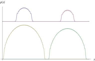
Figure 1: Smoothing out the densities (15); on the upper graph is plotted $\rho^{occ}(n\!=\!20)$ and $\rho^{unocc}(N\!-\!n\!=\!15)$, and on the lower graph is plotted $\rho^{occ}(n\!=\!100)$ and $\rho^{unocc}(N\!-\!n\!=\!80)$, with $g/2\omega^{2}=15$.

In the limit $N-n,n\to\infty$, densities (15) reduce to Wigner’s semicircle laws, as indicated in Fig.(1), with centres separated by $g/\omega^{2}$ in accordance with two-cut solution previously found hl1 . This result shows that in the strong coupling limit we still have well separated densities of occupied and unoccupied levels, although the probability nature of the levels dynamics allows mixing of levels. Furthermore, Eq.(15) shows that in the case of finite number of levels and finite number of fermions there exist states in the previously found homolumo gap hl1 . Note that in precisely this regime, i.e., in the limit of strong interaction, the model defined by (1) was used as a toy model for QCD in the analysis of the spectrum of mesons and baryons Aff .

In the case of weak interaction, up to first order in $g$ we can write the Hamiltonian (1) as

$$H=e^{iH_{fb}}H_{B}e^{-iH_{fb}},$$ (16)

where

$$H_{fb}={g\over 2\omega^{2}}\sum_{l,k}\left(f_{l}^{\dagger}f^{k}-f^{k}f_{l}^{\dagger}\right)P_{k}^{l}.$$ (17)

The eigenstate of the Hamiltonian  (16) is

$$|\Psi\rangle=e^{iH_{fb}}|\Phi\rangle,$$ (18)

where $|\Phi\rangle$ is an eigenstate of $H_{B}$. The density of occupied eigenvalues in this state is

$$\langle\rho^{occ}(x)\rangle = \langle\Psi|\sum_{i}d_{i}^{\dagger}d^{i}\delta(x-x_{i})|\Psi\rangle=$$ (19)

$$= \sum_{i}\langle\Phi|e^{-iH_{fb}}d_{i}^{\dagger}d^{i}\delta(x-x_{i})e^{iH_{fb}}|\Phi\rangle.$$

Expanding in $g$ up to first order we obtain

$$\langle\rho^{occ}(x)\rangle=\langle\rho^{occ}_{0}(x)\rangle+{g\over 2\omega^{2}}\partial_{x}\langle\rho^{occ}_{0}(x)\rangle,$$ (20)

where $\langle\rho^{occ}_{0}(x)\rangle$ is the density of occupied levels for $g=0$. Analogously we find

$$\langle\rho^{unocc}(x)\rangle=\langle\rho^{unocc}_{0}(x)\rangle-{g\over 2\omega^{2}}\partial_{x}\langle\rho^{unocc}_{0}(x)\rangle.$$ (21)

The case of weak interaction shows that starting with the system of bosons determined by the Hamiltonian $H_{B}$, introduction of boson-fermion interaction results in the displacement of the occupied levels by $-g/2\omega^{2}$ and unoccupied levels by $g/2\omega^{2}$, whatever these densities are in the case $g=0$.

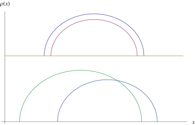
Figure 2: We sketched development of gap in the weak coupling limit for $N-n,n\to\infty$.

Moreover, one can show that even to the second order the boson-fermion interaction results only in the displacement of the of occupied levels by $-g/2\omega^{2}$ and unoccupied levels by $g/2\omega^{2}$. As this is exactly the result of the strong coupling approximation, one might speculate that this would be also true for the intermediate $g$. In that case, in the transition region where densities, although displaced, still overlap, as in Fig(2), the total density of levels in the large $N$ limit (the sum of two semicircle distributions) would display two (ignoring the end-points) homolumo ’kinks’.

The appearance of the gap in our picture depends on the frequency $\omega$, the interaction strength $g$ and the number of levels $N$ and number of fermions $n$. The control over these parameters effectively controls the size of the gap. A possible disappearance of the gap, observed in reality, can be also interpreted within our picture as a consequence of the existence of the several subsystems whose gaps are arranged in appropriate way. Namely, one could introduce different frequencies $\omega_{i}$ in bosonic part of the model, which would result in different gap for each subsystem, and these could be arranged to overlap. This could provide a simple model for exploring the insertion of a single level into the gap.

Furthermore, the Hamiltonian (1) looks exactly as the Hamiltonian used to derive the linear Jahn-Teller effect jt , which says that due to the degeneracy of orbital fermions levels the symmetry of the molecule is broken in the ground state. Although in description of this effect the Hamiltonian (1) is defined in configuration rather than in momentum/energy space, the homolumo gap we observe can be interpreted as manifestation of breaking of gauge symmetry, representing generalisation of Jahn-Teller effect.

In our approach, the crucial point was use of suitable unitary transformation that enabled us to diagonalize the model in both strong and weak coupling approximation. On the other hand, using the conserved ”angular momentum” generators and appropriate spectrum generating algebra, one should attempt to construct exact eigenstates of the system. We hope to report on the related results in future publications.

References

- (1) H. A. Jahn and E. Teller, Proc. Roy. Soc. London A161 (1937) 220; M. Pope and C. E. Swenberg, Electronic Processes in Organic Crystals and Polymers, (2nd ed., Oxford University Press, NY (1999)).
- (2) H. B. Nielsen, “Dual Strings,” in “Scottish Universities Summer School” (1974) in Sct. Andrews; D. L. Bennett, N. Brene and H. B. Nielsen, Phys. Scripta T15 (1987) 158; C. D. Froggatt and H. B. Nielsen, Origin of symmetries, World Scientific (1991); C. D. Froggatt and H. B. Nielsen, Annalen der Physik 14, (2005) 115; see also www.nbi.dk/ kleppe/random/qa/qa.html .
- (3) I. Andrić, L. Jonke, D. Jurman and H. B. Nielsen, Phys. Rev. D 77 (2008) 127701 [arXiv:0712.3760 [hep-th]].
- (4) N. Iizuka and J. Polchinski, JHEP 0810 (2008) 028 [arXiv:0801.3657 [hep-th]].
- (5) I. Affleck, Nucl. Phys. B 185 (1981) 346. J. D. Lykken, Phys. Rev. D 25 (1982) 1653.
- (6) S. Alexandrov, arXiv:hep-th/0311273.
- (7) J. L. Karczmarek and A. Strominger, JHEP 0404 (2004) 055 [arXiv:hep-th/0309138].
- (8) F. Calogero, J. Math. Phys. 10 (1969) 2197; M. A. Olshanetsky, A. M. Perelomov, Phys. Rept. 94 (1983) 313; I. Andrić and D. Jurman, JHEP 0501 (2005) 039 [arXiv:hep-th/ 0411034].
- (9) M. L. Mehta, ”Random Matrices”, (2nd Edition, Academic Press, NY(1991)).
- (10) T. Guhr, A. Mueller-Groeling, H. A. Weidenmueller, Phys. Rept. 299 (1998) 189.