Properly embedded minimal planar domains with infinite topology are Riemann minimal examples

Abstract

These notes outline recent developments in classical minimal surface theory that are essential in classifying the properly embedded minimal planar domains $M\subset\mathbb{R}^{3}$ with infinite topology (equivalently, with an infinite number of ends). This final classification result by Meeks, Pérez, and Ros [64] states that such an $M$ must be congruent to a homothetic scaling of one of the classical examples found by Riemann [87] in 1860. These examples ${\cal R}_{s},0<s<\infty$, are defined in terms of the Weierstrass ${\cal P}$-functions ${\cal P}_{t}$ on the rectangular elliptic curve $\frac{\mathbb{C}}{\langle 1,t\sqrt{-1}\rangle}$, are singly-periodic and intersect each horizontal plane in $\mathbb{R}^{3}$ in a circle or a line parallel to the $x$-axis. Earlier work by Collin [22], López and Ros [49] and Meeks and Rosenberg [71] demonstrate that the plane, the catenoid and the helicoid are the only properly embedded minimal surfaces of genus zero with finite topology (equivalently, with a finite number of ends). Since the surfaces ${\cal R}_{s}$ converge to a catenoid as $s\to 0$ and to a helicoid as $s\to\infty$, then the moduli space ${\cal M}$ of all properly embedded, non-planar, minimal planar domains in $\mathbb{R}^{3}$ is homeomorphic to the closed unit interval $[0,1]$.

Mathematics Subject Classification: Primary 53A10, Secondary 49Q05, 53C42.

1 Introduction.

In the last decade spectacular progress has been made in various aspects of classical minimal surface theory. Some of the successes obtained are the solutions of open problems which have been pursued since the birth of this subject in the 19-th century, while others have opened vast new horizons for future research. Among the first such successes, we would like to highlight the achievement of a deep understanding of topological aspects of proper minimal embeddings in three-space including their complete topological classification [23, 31, 32, 33, 34, 35, 36]. Equally important in this progress has been a comprehensive analysis of the behavior of limits of sequences of embedded minimal surfaces without a priori area or curvature bounds [9, 15, 16, 17, 18], with outstanding applications such as the classification of all simply-connected, properly embedded minimal surfaces [71]. Also, many deep results have been obtained on the subtle relationship between completeness and properness for complete immersed minimal surfaces [2, 29, 50, 51, 52, 53, 79], and how embeddedness introduces a strong dichotomy in this relationship [21, 61]. While all of these results are extremely interesting, they will not be treated in these notes (at least, not in depth) but they do give an idea of the enormous activity within this field; instead, we will explain the recent solution to the following long standing problem in classical minimal surface theory:

Classify all possible properly embedded minimal surfaces of genus zero in $\mathbb{R}^{3}$.

Research by various authors help to understand this problem, the more relevant work being by Colding and Minicozzi [18, 21], Collin [22], López and Ros [49], Meeks, Pérez and Ros [64] and Meeks and Rosenberg [70, 71]. In fact, this problem has been one of main goals of the two authors of these notes (in collaboration with A. Ros) for over the past 15 years, and the long path towards its solution has been marked by the discovery of powerful techniques which have proved useful in other applications. Putting together all of these efforts, we now state the final solution to the above problem, whose proof appears in [64].

Theorem 1.1

Up to scaling and rigid motion, any connected, properly embedded, minimal planar domain in $\mathbb{R}^{3}$ is a plane, a helicoid, a catenoid or one of the Riemann minimal examples. In particular, for every such surface there exists a foliation of $\mathbb{R}^{3}$ by parallel planes, where each plane intersects the surface transversely in a circle or a straight line.

In these notes we will try to pass on to the reader a glimpse of the beauty of the arguments and different theories that intervene in the proof of Theorem 1.1. Among these auxiliary theories, we highlight the theory of integrable systems, whose applications to minimal and constant mean curvature surface theory have gone far beyond the existence results in the late eighties (Abresch [1], Bobenko [5], Pinkall and Sterling [85], based on the sinh-Gordon equation) to recent uniqueness theorems like the one that gives the title of these notes (based on the KdV equation), and the even more recent tentative solution to the Lawson conjecture by Kilian and Schmidt [45].

Before proceeding, we make a few general comments about the organization of this article, which relate to the proof of Theorem 1.1. In Section 2 we briefly introduce the main definitions and background material, including short discussions of the classical examples that appear in the statement of the above theorem. Since a complete, immersed minimal surface $M$ without boundary in $\mathbb{R}^{3}$ cannot be compact, $M$ must have ends. As we are interested in planar domains, the allowed topology for our surfaces in that of the two-sphere minus a compact totally disconnected set ${\cal E}\neq\mbox{\O}$ corresponding to the space of ends of the surface. A crucial result proved by Collin [22] in 1997 (see Conjecture 3.3 below) implies that when the cardinality $\#({\cal E})$ of ${\cal E}$ satisfies $2\leq\#({\cal E})<\infty$, then the total Gaussian curvature of $M$ is finite. Complete embedded minimal surfaces with finite total curvature comprise the best understood minimal surfaces in $\mathbb{R}^{3}$; the main reason for this is the fact discovered by Osserman that the underlying complex structure for every such minimal surface $M$ is that of a compact Riemann $\overline{M}$ surface minus a finite number of points, and the classical analytic Weierstrass representation data on $M$ extends across the punctures to meromorphic data on $\overline{M}$. Using the maximum principle together with their result that every complete, embedded minimal surface with genus zero and finite total curvature can be minimally deformed, López and Ros characterized the plane and the catenoid as being the unique embedded examples of finite total curvature and genus zero, see Theorem 3.2. We also explain Collin’s and López-Ros’ theorems in Section 3.

Section 4 covers the one-ended case of Theorem 1.1, which was solved by Meeks and Rosenberg (Theorem 4.2). To understand the proof of this result we need the local results of Colding and Minicozzi which describe the structure of compact, embedded minimal disks as essentially being modeled by either a plane or a helicoid, and their one-sided curvature estimate together with other results of a global nature such as their limit lamination theorem for disks, see Theorem 4.1 below.

The remainder of the article, except for the last section, focuses on the case in Theorem 1.1 where the surface has infinitely many ends. Crucial in this discussion is the Ordering Theorem by Frohman and Meeks (Theorem 5.1) as well as two topological results, the first on the non-existence of middle limit ends due to Collin, Kusner, Meeks and Rosenberg (Theorem 5.3) and the second on the non-existence of properly embedded minimal planar domains with just one limit end by Meeks, Pérez and Ros (Theorem 5.11). It follows from these two non-existence results that a properly embedded minimal planar domain must have exactly two limit ends. These key ingredients represent the content of Section 5.

As a consequence of the results in Section 5, in Section 6 we obtain strong control on the conformal structure and height differential of a properly embedded, minimal planar domain $M$ with infinitely many ends. In this section we also explain how Colding-Minicozzi theory can be applied to obtain a curvature bound for such an $M$, after it has been the normalized by a homothety so that its vertical flux is $1$, which only depends on the length of the horizontal component of its flux vector (Theorem 6.3). This bound leads to a quasi-periodicity property of $M$, which is a cornerstone to finishing the classification problem. Also in Section 6 we introduce the Shiffman Jacobi function $S_{M}$ and explain how the existence of a related holomorphic deformation of $M$ preserving its flux is sufficient to reduce the proof of Theorem 1.1 in the case with infinitely many ends to the singly-periodic case, which was solved earlier by Meeks, Pérez and Ros [66].

In Section 7 we explain how the existence of the desired holomorphic deformation of $M$ follows from the integration of an evolution equation for its Gauss map. The Shiffman function $S_{M}$ will be crucial at this point by enabling us to reduce this evolution equation to an equation of type Korteweg de Vries (KdV). A classical condition that implies global integrability of the KdV equation, i.e. existence of (globally defined) meromorphic solutions $u(z,t)$ of the Cauchy problem associated to the KdV equation, is that the initial condition $u(z)$ is an algebro-geometric meromorphic function, a concept related to the hierarchy of the KdV equation. In our setting, the final step of the classification of the properly embedded minimal planar domains consists of proving that the initial condition $u(z)$ for the Cauchy problem of the KdV equation naturally associated to any quasiperiodic, possibly immersed, minimal planar domain $M$ with two limit ends is algebro-geometric (Section 7.4), which in turn is a consequence of the fact that the space of bounded Jacobi functions on such a surface $M$ is finite dimensional (Theorem 7.3).

An important consequence of the proof of the classification of properly embedded minimal planar domains is the characterization of the asymptotic behavior of the ends of any properly embedded minimal surface $M\subset\mathbb{R}^{3}$ with finite genus. If $e\in{\cal E}(M)$ is an end, then there exists properly embedded domain $E(e)\subset M$ with compact boundary which represents $e$ and such that in a natural sense $E(e)$ converges to the end of a plane, a catenoid, a helicoid or to one of the limit ends of a Riemann minimal example. This asymptotic characterization is due to Schoen [91] and Collin [22] when $M$ has a finite number of ends greater than one, to Meeks, Pérez and Ros in the case $M$ has an infinite number of ends, and to Meeks and Rosenberg [71], Bernstein and Breiner [3], and Meeks and Pérez [58, 59] in the case of just one end. These asymptotic characterization results will be explained in Section 8 of these notes.

2 Background.

An isometric immersion $X=(x_{1},x_{2},x_{3})\colon M\to\mathbb{R}^{3}$ of a Riemannian surface into Euclidean space is said to be minimal if $x_{i}$ is a harmonic function on $M$ for each $i$ (in the sequel, we will identify the Riemannian surface $M$ with its image under the isometric embedding). Since harmonicity is a local property, we can extend the notion of minimality to immersed surfaces $M\subset\mathbb{R}^{3}$. We will always assume all surfaces under consideration are orientable. If $M\subset\mathbb{R}^{3}$ is an immersed oriented surface, we will denote by $H$ the mean curvature function of $X$ (average normal curvature) and by $N\colon M\to\mathbb{S}^{2}(1)\subset\mathbb{R}^{3}$ its Gauss map. Since $\Delta X=2HN$ (here $\Delta$ is the Laplace-Beltrami operator on $M$), we have that $M$ is minimal if and only if $H=0$ identically. Expressing locally $M$ as the graph of a function $u=u(x,y)$ (after a rotation), the last equation can be written as the following quasilinear second order elliptic PDE:

$$\mbox{\rm div}_{0}\left(\frac{\nabla_{0}u}{\sqrt{1+|\nabla_{0}u|^{2}}}\right)=0,$$ (1)

where the subscript $\bullet_{0}$ indicates that the corresponding object is computed with respect to the flat metric in the plane.

Let $\Omega$ be a subdomain with compact closure in a surface $M\subset\mathbb{R}^{3}$ and let $u\in C^{\infty}_{0}(\Omega)$ be a compactly supported smooth function. The first variation of the area functional $A(t)=\mbox{Area}((X+tuN)(\Omega))$ for the normally perturbed immersions $X+utN$ (with $|t|$ sufficiently small) gives

$$A^{\prime}(0)=-2\int_{\Omega}uH\,dA,$$ (2)

where $dA$ stands for the area element of $M$. Therefore, $M$ is minimal if and only if it is a critical point of the area functional for all compactly supported variations. The second variation of area implies that any point in a minimal surface has a neighborhood with least-area relative to its boundary, and thus $M\subset\mathbb{R}^{3}$ is minimal if and only if every point $p\in M$ has a neighborhood with least-area relative to its boundary. If one exchanges the area functional $A$ by the Dirichlet energy $E=\int_{\Omega}|\nabla X|^{2}dA$, then the two functionals are related by $E\geq 2A$, with equality if and only if the immersion $X\colon M\to\mathbb{R}^{3}$ is conformal. This relation between area and energy together with the existence of isothermal coordinates on every Riemannian surface allow us to state that a conformal immersion $X\colon M\to\mathbb{R}^{3}$ is minimal if and only if it is a critical point of the Dirichlet energy for all compactly supported variations (or equivalently, every point $p\in M$ has a neighborhood with least energy relative to its boundary). Finally, the relation $A_{p}=-dN_{p}$ between the differential of the Gauss map and the shape operator, together with the Cauchy-Riemann equations give that $M$ is minimal if and only if its stereographically projected Gauss map $g\colon M\to\mathbb{C}\cup\{\infty\}$ is a holomorphic function. All these equivalent definitions of minimality illustrate the wide variety of branches of mathematics that appear in its study: Differential Geometry, PDE, Calculus of Variations, Geometric Measure Theory, Complex Analysis, etc.

The Gaussian curvature function $K$ of a surface $M\subset\mathbb{R}^{3}$ can be written as $K=\kappa_{1}\kappa_{2}=\det A$, where $\kappa_{i}$ are the principal curvatures and $A$ the shape operator. Thus $|K|$ is the absolute value of the Jacobian of the Gauss map $N$. If $M$ is minimal, then $\kappa_{1}=-\kappa_{2}$ and $K\leq 0$, hence the total curvature $C(M)$ of $M$ is the negative of the spherical area of $M$ through its Gauss map, counting multiplicities:

$$C(M)=\int_{M}K\,dA=-{\rm Area}(N\colon M\rightarrow\mathbb{S}^{2}(1))\in[-\infty,0].$$ (3)

In the sequel, we will denote by $\mathbb{B}(p,R)=\{x\in\mathbb{R}^{3}\ |\ |x-p|<R\}$ and $\mathbb{B}(R)=\mathbb{B}(\vec{0},R)$.

2.1 Weierstrass representation and the definition of flux.

Let $M\subset\mathbb{R}^{3}$ be a possibly immersed minimal surface, with stereographically projected Gauss map $g\colon M\to\mathbb{C}\cup\{\infty\}$. Since the third coordinate function $x_{3}$ of $M$ is harmonic, it admits a locally well-defined harmonic conjugate function $x_{3}^{*}$. The height differential of $M$ is the holomorphic 1-form $dh=dx_{3}+idx_{3}^{*}$ (note that $dh$ is not necessarily exact on $M$). The minimal immersion $X\colon M\to\mathbb{R}^{3}$ can be written up to translation by the vector $X(p_{0})$, $p_{0}\in M$, solely in terms of the Weierstrass data $(g,dh)$ as

$$X(p)=\Re\int_{p_{0}}^{p}\left(\frac{1}{2}\left(\frac{1}{g}-g\right),\frac{i}{2}\left(\frac{1}{g}+g\right),1\right)dh,$$ (4)

where $\Re$ stands for real part. The positive-definiteness of the induced metric and the independence of (4) with respect to the integration path give rise to certain compatibility conditions on the meromorphic data $(g,dh)$ for analytically defining a minimal surface (Osserman [80]); namely, if we start with a meromorphic function $g$ and a holomorphic one-form $dh$ on an abstract Riemann surface $M$, then the map $X\colon M\to\mathbb{R}^{3}$ given by (4) is a conformal minimal immersion with Weierstrass data $(g,dh)$ provided that two conditions hold:

The zeros of $$dh g$$ coincide with the poles and zeros of , with the same order. (5)

$$\overline{\int_{{\gamma}}g\,dh}=\int_{{\gamma}}\frac{dh}{g},\quad\Re\int_{{\gamma}}dh=0\ \mbox{ for any closed curve ${\gamma}\subset M$ (period problem).}$$ (6)

The flux vector of $M$ along a closed curve ${\gamma}\subset M$ is defined as

$$F(\gamma)=\int_{\gamma}\mbox{Rot}_{90^{\circ}}({\gamma}^{\prime})=\Im\int_{{\gamma}}\left(\frac{1}{2}\left(\frac{1}{g}-g\right),\frac{i}{2}\left(\frac{1}{g}+g\right),1\right)dh\in\mathbb{R}^{3},$$ (7)

where $\mbox{Rot}_{90^{\circ}}$ denotes the counterclockwise rotation by angle $\pi/2$ in the tangent plane of $M$ at any point, and $\Im$ stands for imaginary part. Both the period condition (6) and the flux vector (7) only depend on the homology class of ${\gamma}$ in $M$.

2.2 Maximum principles.

Since minimal surfaces can be written locally as solutions of the PDE (1), they satisfy certain maximum principles.

Theorem 2.1 (Interior and boundary maximum principles [91])

Let $M_{1},M_{2}$ be connected minimal surfaces in $\mathbb{R}^{3}$ and $p$ an interior point to both surfaces, such that $T_{p}M_{1}=T_{p}M_{2}=\{x_{3}=0\}$. If $M_{1},M_{2}$ are locally expressed as the graphs of functions $u_{1},u_{2}$ around $p$ and $u_{1}\leq u_{2}$ in a neighborhood of $p$, then $M_{1}=M_{2}$ in a neighborhood of $p$. The same conclusion holds if $p$ is a boundary point of both surfaces and additionally, $T_{p}\partial M_{1}=T_{p}\partial M_{2}$.

We also dispose of more sophisticated versions of the maximum principle, where a first contact point of two minimal surfaces does not occur at a finite point but at infinity, amongst which we state two. The first one (whose proof we sketch for later purposes) was proved by Hoffman and Meeks, and the second one is due to Meeks and Rosenberg.

Theorem 2.2 (Half-space Theorem [41])

A properly immersed, non-planar minimal surface without boundary cannot be contained in a half-space.

Sketch of proof. Arguing by contradiction, suppose that a surface $M\subset\mathbb{R}^{3}$ as in the hypotheses is contained in $\{x_{3}\geq 0\}$ (and so, $M\subset\{x_{3}>0\}$ by Theorem 2.1) but is not contained in $\{x_{3}>c\}$ for any $c>0$. Since $M$ is proper, we can find a ball $\mathbb{B}(p,r)$ centered at a point $p\in\{x_{3}=0\}$ such that $M\cap\mathbb{B}(p,r)=\mbox{\O}$. Consider a vertical half-catenoid $C$ with negative logarithmic growth, completely contained in $\{x_{3}\leq 0\}\cup\mathbb{B}(p,r)$, whose waist circle ${\Gamma}$ is centered at $q=p+{\varepsilon}(0,0,1)$, ${\varepsilon}>0$ small. Then $M\cap C=\mbox{\O}$. Now deform $C=C(1)$ by a one-parameter family of non-compact annular pieces of vertical catenoids $\{C(r)\}_{r\in(0,1]}$, all having the same boundary ${\Gamma}$ as $C$, with negative logarithmic growths converging to zero as $r\to 0$ and whose Gaussian curvatures blow up at a the limit point of the waist circles of $C(r)$, which is the point $q$. Then, the surfaces $C(r)$ converge on compact subsets of $\mathbb{R}^{3}-\{q\}$ to the plane $\{x_{3}={\varepsilon}\}$, and so, $M$ achieves a first contact point with one of the catenoids, say $C(r_{0})$, in this family; the usual maximum principle for $M$ and $C(r_{0})$ gives a contradiction. $\Box$

Theorem 2.3 (Maximum Principle at Infinity [73])

Let $M_{1},M_{2}\subset\mathbb{R}^{3}$ be disjoint, connected, properly immersed minimal surfaces with (possibly empty) boundary.

• If $\partial M_{1}\neq\mbox{\rm\O}$ or $\partial M_{2}\neq\mbox{\rm\O}$, then after possibly re-indexing,

  $${\rm dist}(M_{1},M_{2})=\inf\{{\rm dist}(p,q)\mid p\in\partial M_{1},\,q\in M_{2}\}.$$

• If $\partial M_{1}=\partial M_{2}=\mbox{\rm\O}$, then $M_{1}$ and $M_{2}$ are flat.

2.3 Monotonicity formula.

Monotonicity formulas, as well as maximum principles, play a crucial role in many areas of Geometric Analysis. For instance, we will see in Theorem 5.3 how the monotonicity formula can be used to discard middle limit ends for a properly embedded minimal surface. We will state this basic result without proof here; it is a consequence of the classical coarea formula applied to the distance function to a point $p\in\mathbb{R}^{3}$, see for instance Corollary 4.2 in [14] for a detailed proof.

Theorem 2.4 (Monotonicity Formula [10, 46])

Let $X\colon M\to\mathbb{R}^{3}$ be a connected, properly immersed minimal surface. Given $p\in\mathbb{R}^{3}$, let $A(R)=\mbox{\rm Area}(X(M)\cap\mathbb{B}(p,R))$. Then, $A(R)R^{-2}$ is non-decreasing. In particular, $\lim_{R\to\infty}A(R)R^{-2}\geq\pi$ with equality if and only if $M$ is a plane.

2.4 Stability, Plateau problem and barrier constructions.

Recall that every (orientable) minimal surface $M\subset\mathbb{R}^{3}$ is a critical point of the area functional for compactly supported normal variations. $M$ is said to be stable if it is a local minimum for such a variational problem. The following well-known result indicates how restrictive is stability for complete minimal surfaces. It was proved independently by Fischer-Colbrie and Schoen [30], do Carmo and Peng [25], and Pogorelov [86] for orientable surfaces and more recently by Ros [89] in the case of non-orientable surfaces.

Theorem 2.5

If $M\subset\mathbb{R}^{3}$ is a complete, immersed, stable minimal surface, then $M$ is a plane.

The Plateau Problem consists of finding a compact surface of least area spanning a given boundary. This problem can be solved under certain circumstances; this existence of compact solutions together with a taking limits procedure leads to construct non-compact stable minimal surfaces in $\mathbb{R}^{3}$ that are constrained to lie in regions of space whose boundaries have non-negative mean curvature. A huge amount of literature is devoted to this procedure, but we will state here only a particular version.

Let $W$ be a compact Riemannian three-manifold with boundary which embeds in the interior of another Riemannian three-manifold. $W$ is said to have piecewise smooth, mean convex boundary if $\partial W$ is a two-dimensional complex consisting of a finite number of smooth, two-dimensional compact simplices with interior angles less than or equal to $\pi$, each one with non-negative mean curvature with respect to the inward pointing normal. In this situation, the boundary of $W$ is a good barrier for solving Plateau problems in the following sense:

Theorem 2.6 ([54, 75, 76, 94])

Let $W$ be a compact Riemannian three-manifold with piecewise smooth mean convex boundary. Let ${\Gamma}$ be a smooth collection of pairwise disjoint closed curves in $\partial W$, which bounds a compact orientable surface in $W$. Then, there exists an embedded orientable surface $\Sigma\subset W$ with $\partial\Sigma={\Gamma}$ that minimizes area among all orientable surfaces with the same boundary.

Instead of giving an idea of the proof of Theorem 2.6, we will illustrate it together with a taking limits procedure to obtain a particular result in the non-compact setting. Consider two disjoint, connected, properly embedded minimal surfaces $M_{1},M_{2}$ in $\mathbb{R}^{3}$ and let $W$ be the closed complement of $M_{1}\cup M_{2}$ in $\mathbb{R}^{3}$ that has both $M_{1}$ and $M_{2}$ on its boundary.

1. We first show how to produce compact, least-area surfaces in $W$ with prescribed boundary lying in the boundary $\partial W$. Note that $W$ is a complete flat three-manifold with boundary, and $\partial W$ has mean curvature zero. Meeks and Yau [76] proved that $W$ embeds isometrically in a homogeneously regular Riemannian three-manifold $\widetilde{W}$ diffeomorphic to the interior of $W$ and with metric $\widetilde{g}$. Morrey [78] proved that in a homogeneously regular manifold, one can solve the classical Plateau problem. In particular, if $\Gamma$ is an embedded $1$-cycle in $\widetilde{W}$ which bounds an orientable finite sum of differentiable simplices in $\widetilde{W}$, then by standard results in geometric measure theory [28], $\Gamma$ is the boundary of a compact, least-area embedded surface $\Sigma_{\Gamma}(\widetilde{g})\subset\widetilde{W}$. Meeks and Yau proved that the metric $\widetilde{g}$ on $\widetilde{W}$ can be approximated by a family of homogeneously regular metrics $\{g_{n}\}_{n\in\mathbb{N}}$ on $\widetilde{W}$, which converges smoothly on compact subsets of $\widetilde{W}$ to $\widetilde{g}$, and each $g_{n}$ satisfies a convexity condition outside of $W\subset\widetilde{W}$, which forces the least-area surface $\Sigma_{\Gamma}(g_{n})$ to lie in $W$ if $\Gamma$ lies in $W$. A subsequence of the $\Sigma_{\Gamma}(g_{n})$ converges to a smooth minimal surface $\Sigma_{\Gamma}$ of least-area in $W$ with respect to the original flat metric, thereby finishing our description of how to solve (compact) Plateau-type problems in $W$.

2. We now describe the limit procedure to construct a non-compact, stable minimal surface with prescribed boundary lying in $M_{1}$. Let $M_{1}(1)\subset\ldots\subset M_{1}(n)\subset\ldots$ be a compact exhaustion of $M_{1}$, and let $\Sigma_{1}(n)$ be a least-area surface in $W$ with boundary $\partial M_{1}(n)$, constructed as in the last paragraph. Let $\alpha$ be a compact arc in $W$ which joins a point in $M_{1}(1)$ to a point in $\partial W\cap M_{2}$. By elementary intersection theory, $\alpha$ intersects every least-area surface $\Sigma_{1}(n)$. By compactness of least-area surfaces, a subsequence of the surfaces $\Sigma_{1}(n)$ converges to a properly embedded area-minimizing surface $\Sigma$ in $W$ with a component $\Sigma_{0}$ which intersects $\alpha$; this proof of the existence of $\Sigma$ is due to Meeks, Simon and Yau [74].

3. We finish this application of the barrier construction, as follows. Since $\Sigma_{0}$ separates $\mathbb{R}^{3}$, $\Sigma_{0}$ is orientable and so, Theorem 2.5 insures that $\Sigma_{0}$ is a plane. Hence, $M_{1}$ and $M_{2}$ lie in closed half-spaces of $\mathbb{R}^{3}$, and the Half-space Theorem (Theorem 2.2) implies that both $M_{1},M_{2}$ are planes.

The above items 1–3 give the following generalization of Theorem 2.2, also due to Hoffman and Meeks.

Theorem 2.7 (Strong Half-space Theorem [41])

If $M_{1}$ and $M_{2}$ are two disjoint, properly immersed minimal surfaces in $\mathbb{R}^{3}$, then $M_{1}$ and $M_{2}$ are parallel planes.

2.5 The examples that appear in Theorem 1.1.

We will now use the Weierstrass representation for introducing the minimal planar domains characterized in Theorem 1.1.

The plane. $M=\mathbb{C}$, $g(z)=1$, $dh=dz$. It is the only complete, flat minimal surface in $\mathbb{R}^{3}$.

The catenoid. $M=\mathbb{C}-\{0\}$, $g(z)=z$, $dh=\frac{dz}{z}$ (Figure 1 left). This surface has genus zero, two ends and total curvature $-4\pi$. Together with the plane, the catenoid is the only minimal surface of revolution (Bonnet [6]). As we will see in Theorem 3.2, the catenoid and the plane are the unique complete, embedded minimal surfaces with genus zero and finite total curvature. Also, the catenoid was characterized by Schoen [91] as being the unique complete, immersed minimal surface with finite total curvature and two embedded ends.

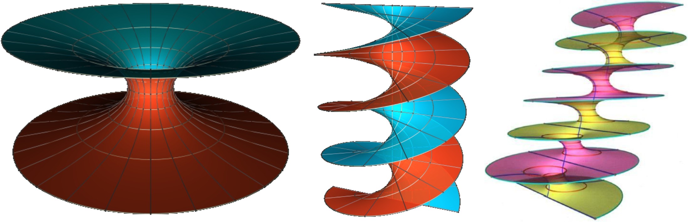
Figure 1: Left: Catenoid. Center: Helicoid. Right: One of the Riemann minimal examples. Figures courtesy of Matthias Weber.

The helicoid. $M=\mathbb{C}$, $g(z)=e^{z}$, $dh=i\,dz$ (Figure 1 center). When viewed in $\mathbb{R}^{3}$, the helicoid has genus zero, one end and infinite total curvature. Together with the plane, the helicoid is the only ruled minimal surface (Catalan [8]), and we will see in Theorem 4.2 below that it is the unique properly embedded, simply-connected minimal surface. The vertical helicoid is invariant by a vertical translation $T$ and by a 1-parameter family of screw motions $S_{\theta}$, $\theta>0$. Viewed in $\mathbb{R}^{3}/T$ or in $\mathbb{R}^{3}/S_{{\theta}}$, the helicoid is a properly embedded minimal surface with genus zero, two ends and finite total curvature. The catenoid and the helicoid are conjugate minimal surfaces, in the sense that the coordinate functions of one of these surfaces are the harmonic conjugates of the coordinate functions of the other one; in this case, we consider the catenoid to be defined on its universal cover $e^{z}\colon\mathbb{C}\rightarrow\mathbb{C}-\{0\}$ in order for the harmonic conjugate of $x_{3}$ to be well-defined.

The Riemann minimal examples. They form a one-parameter family, with Weierstrass data $M_{\lambda}=\{(z,w)\in(\mathbb{C}\cup\{\infty\})^{2}\ |\ w^{2}=z(z-\lambda)(\lambda z+1)\}-\{(0,0),(\infty,\infty)\}$, $g(z,w)=z$, $dh=A_{\lambda}\frac{dz}{w}$, for each ${\lambda}>0$, where $A_{\lambda}$ is a non-zero complex number satisfying $A_{\lambda}^{2}\in\mathbb{R}$ (one of these surfaces is represented in Figure 1 right). Together with the plane, catenoid and helicoid, these examples were characterized by Riemann [88] as the unique minimal surfaces which are foliated by circles and lines in parallel planes. Each Riemann minimal example $M_{{\lambda}}$ is topologically a cylinder minus an infinite set of points which accumulates at infinity to the top or bottom ends of the cylinder; hence, $M_{{\lambda}}$ is topologically the unique planar domain with two limit ends. Furthermore, $M_{{\lambda}}$ is invariant under reflection in the $(x_{1},x_{3})$-plane and by a translation $T_{{\lambda}}$; the quotient surface $M_{{\lambda}}/T_{{\lambda}}\subset\mathbb{R}^{3}/T_{{\lambda}}$ has genus one and two planar ends, provided that $T_{{\lambda}}$ is the generator of the orientation preserving translations of $M_{\lambda}$. The conjugate minimal surface of $M_{{\lambda}}$ is $M_{1/{\lambda}}$ (the case ${\lambda}=1$ gives the only self-conjugate surface in the family). See [64] for a more precise description of these surfaces.

3 The case with $r$ ends, $2\leq r<\infty$.

Complete minimal surfaces with finite total curvature can be naturally thought of as compact algebraic objects, which explains why these surfaces form the most extensively studied family among complete minimal surfaces.

Theorem 3.1 (Huber [42], Osserman [81])

Let $M\subset\mathbb{R}^{3}$ be a complete (oriented), immersed minimal surface with finite total curvature. Then, $M$ is conformally a compact Riemann surface $\overline{M}$ minus a finite number of points, and the Weierstrass representation $(g,dh)$ of $M$ extends meromorphically to $\overline{M}$. In particular, the total curvature of $M$ is a multiple of $-4\pi$.

Under the hypotheses of the last theorem, the Gauss map $g$ has a well-defined finite degree on $\overline{M}$, and equation (3) implies that the total curvature of $M$ is $-4\pi$ times the degree of $g$. The Gauss-Bonnet formula relates the degree of $g$ with the genus of $\overline{M}$ and the number of ends (Jorge and Meeks [43]); although this formula can be stated in the more general immersed case, we will only consider it when all the ends of $M$ are embedded:

$$\mbox{deg}(g)=\mbox{genus}(\overline{M})+\#(\mbox{ends})-1.$$ (8)

The asymptotics of a complete, embedded minimal surface in $\mathbb{R}^{3}$ with finite total curvature are also well-understood: after a rotation, each embedded end of such a surface is a graph over the exterior of a disk in the $(x_{1},x_{2})$-plane with height function

$$x_{3}(x_{1},x_{2})=a\log r+b+\frac{c_{1}x_{1}+c_{2}x_{2}}{r^{2}}+{\mathcal{O}}(r^{-2}),$$ (9)

where $r=\sqrt{x_{1}^{2}+x_{2}^{2}}$, $a,b,c_{1},c_{2}\in\mathbb{R}$ and ${\mathcal{O}}(r^{-2})$ denotes a function such that $r^{2}{\mathcal{O}}(r^{-2})$ is bounded as $r\to\infty$ (Schoen [91]). When the logarithmic growth $a$ in (9) is not zero, the end is called a catenoidal end (and the surface is asymptotic to a half-catenoid); if $a=0$, we have a planar end (and the surface is asymptotic to a plane). A consequence of the asymptotics (9) is that for minimal surfaces with finite total curvature, completeness is equivalent to properness (this is also true for immersed surfaces).

The classification of the complete embedded minimal surfaces with genus zero and finite total curvature in $\mathbb{R}^{3}$ was solved in 1991 by López and Ros [49]. Their result is based on the fact that every surface in this family can be deformed through minimal surfaces of the same type; this is a strong property which we will encounter in more general situations, as in Theorem 6.11 below.

In the finite total curvature setting, the deformation is explicitly given in terms of the Weierstrass representation: If $(g,dh)$ is the Weierstrass pair of a minimal surface $M$, then for each ${\lambda}>0$ the pair $({\lambda}g,dh)$ satisfies condition (5) and the second equation in (6). The first equation in (6) holds for $({\lambda}g,dh)$ provided that the flux vector $F({\gamma})$ of $M$ along every closed curve ${\gamma}\subset M$ is vertical. If $M$ is assumed to have genus zero and finite total curvature, then the homology classes of $M$ are generated by loops around its planar and/or catenoidal ends. It is easy to check that the flux vector of a catenoidal (resp. planar) end along a non-trivial loop is $(0,0,\pm 2\pi a)$ after assuming that the limiting normal vector at the end is $(0,0,\pm 1)$. Since embeddedness implies that all the ends are parallel, then all the flux vectors of our complete embedded minimal surface $M$ with genus zero and finite total curvature are vertical; hence $({\lambda}g,dh)$ defines a minimal immersion $X_{{\lambda}}$ by the formula (4) for each ${\lambda}>0$; note that for ${\lambda}=1$ we obtain the starting surface $M$.

A direct consequence of the maximum principle is that smooth deformations of compact minimal surfaces remain embedded away from their boundaries. The strong control on the asymptotics for complete embedded minimal surfaces of finite total curvature implies embeddedness throughout the entire deformation $\{X_{{\lambda}}\}_{{\lambda}>0}$. This last property excludes both points in $M$ with horizontal tangent plane and planar ends (a local analysis of the deformation around such points and ends produce self-intersections in $X_{{\lambda}}$ for values of the parameter ${\lambda}$ close to zero or infinity), which in turn implies that the height function $x_{3}$ of $M$ is proper without critical points. A simple application of Morse theory gives that $M$ has just two ends, in which case the characterization of the catenoid was previously solved by Schoen [91]. This is a sketch of the proof of the following result.

Theorem 3.2 (López, Ros [49])

The plane and the catenoid are the only complete, embedded minimal surfaces in $\mathbb{R}^{3}$ with genus zero and finite total curvature.

The next step in our classification of all properly embedded minimal planar domains is to understand the case when the number of ends is finite and at least two. In 1993, Meeks and Rosenberg [70] showed that if a properly embedded minimal surface $M\subset\mathbb{R}^{3}$ has at least two ends, then every annular end $E\subset M$ either has finite total curvature or it satisfies the hypotheses of the following conjecture, which was solved by Collin in 1997.

Conjecture 3.3 (Generalized Nitsche Conjecture, Collin’s Theorem [22])

Let $E\subset\{x_{3}\geq 0\}$ be a properly embedded minimal annulus with $\partial E\subset\{x_{3}=0\}$, such that $E$ intersects each plane $\{x_{3}=t\}$, $t>0$, in a simple closed curve. Then, $E$ has finite total curvature.

As a direct consequence of the last result and Theorem 3.2, we have that the plane and the catenoid are the unique properly embedded minimal surfaces in $\mathbb{R}^{3}$ with genus zero and $r$ ends, $2\leq r<\infty$.

Collin’s original proof of Conjecture 3.3 is a beautiful and long argument based on the construction of auxiliary minimal graphs which serve as guide posts to elucidate the shape of $E$ in space. For later purposes, it will be more useful for us to briefly explain a later proof due to Colding and Minicozzi, which is based on the following scale invariant bound for the Gaussian curvature of any embedded minimal disk in a half-space.

Theorem 3.4 (One-sided curvature estimates, Colding, Minicozzi [18])

There exists ${\varepsilon}>0$ such that the following holds. Given $r>0$ and an embedded minimal disk $M\subset\mathbb{B}(2r)\cap\{x_{3}>0\}$ with $\partial M\subset\partial\mathbb{B}(2r)$, then for any component $M^{\prime}$ of $M\cap\mathbb{B}(r)$ which intersects $\mathbb{B}({\varepsilon}r)$,

$$\sup_{M^{\prime}}|K_{M}|\leq r^{-2}.$$

Before sketching the proof of the Nitsche Conjecture, we will make a few comments about the one-side curvature estimates. The catenoid shows that the hypothesis in Theorem 3.4 on $M$ to be simply-connected is necessary. Theorem 3.4 implies that if an embedded minimal disk is close enough to (and lies at one side of) a plane, then reasonably large components of it are graphs over this plane. The proof of Theorem 3.4 is long and delicate, see [15, 16, 18].

Returning to the Nitsche Conjecture, we see that it follows directly from the next result. Given ${\varepsilon}\in\mathbb{R}$, we denote by ${\mathcal{C}}_{{\varepsilon}}$ the conical region $\{x_{3}>{\varepsilon}\sqrt{x_{1}^{2}+x_{2}^{2}}\}$.

Theorem 3.5 (Colding, Minicozzi [11])

There exists ${\delta}>0$ such that any properly embedded minimal annular end $E\subset{\mathcal{C}}_{-{\delta}}$ has finite total curvature.

Sketch of proof of Theorem 3.5. The argument starts by showing, for each ${\delta}>0$, the existence of a sequence $\{y_{j}\}_{j}\subset E-{\mathcal{C}}_{{\delta}}$ with $\|y_{j}\|\to\infty$ (this is done by contradiction: if for a given ${\delta}>0$ this property fails, then one use $E$ together with the boundary of ${\mathcal{C}}_{{\delta}}$ as barriers to construct an end of finite total curvature contained in ${\mathcal{C}}_{{\delta}}$, which is clearly impossible by the controlled asymptotics of catenoidal and planar ends). The next step consists of choosing suitable radii $r_{j}>0$ such that the connected component $M_{j}$ of $E\cap\mathbb{B}(y_{j},2r_{j})$ which contains $y_{j}$ is a disk. Now if ${\delta}>0$ is sufficiently small in terms of the ${\varepsilon}$ appearing in the one-sided curvature estimates, we can apply Theorem 3.4 and conclude a bound for the supremum of the absolute Gaussian curvature of the component $M_{j}^{1}$ of $M_{j}\cap\mathbb{B}(y_{j},r_{j})$ which contains $y_{j}$. A Harnack type inequality together with this curvature bound gives a bound for the length of the intrinsic gradient of $x_{3}$ in the intrinsic ball ${\mathcal{B}}_{j}$ in $M_{j}^{1}$ centered at $y_{j}$ with radius $5r_{j}/8$, which in turn implies (by choosing ${\varepsilon}$ sufficiently small) that ${\mathcal{B}}_{j}$ is a graph with small gradient over $x_{3}=0$, and one can control a bound by below of the diameter of this graph. This allows to repeat the above argument exchanging $y_{j}$ by a point $y_{j}^{1}$ in ${\mathcal{B}}_{j}^{1}$ at certain distance from $y_{j}$, and the estimates are carefully done so that the procedure can be iterated to go entirely around a curve ${\gamma}_{j}\subset E$ whose projection to the $(x_{1},x_{2})$-plane links once around the $x_{3}$-axis. The graphical property of ${\gamma}_{j}$ implies that either ${\gamma}_{j}$ can be continued inside $E$ to spiral indefinitely or it closes up with linking number one with the $x_{3}$-axis. The first possibility contradicts that $E$ is properly embedded, and in the second case the topology of $E$ implies that $\partial E\cup{\gamma}_{j}$ bounds an annulus $E_{j}$. The above gradient estimate gives a linear growth estimate for the length of ${\gamma}_{j}$ in terms of $\|y_{j}\|$, from where the isoperimetric inequality for doubly connected minimal surfaces by Osserman and Schiffer [82] gives a quadratic growth estimate for the area of $E_{j}$. Finally, this quadratic area growth property together with the finiteness of the topology of $E$ imply that $E$ has finite total curvature by the Gauss-Bonnet formula, finishing the outline of proof.

4 The one-ended case.

In our goal of classifying the properly embedded minimal surfaces with genus zero, the simplest topology occurs when the number of ends is one, and the surface is simply-connected. In spite of this apparent simplicity, this problem remained open until 2005, when Meeks and Rosenberg gave a complete solution by using the one-side curvature estimates (Theorem 3.4) and other aspects of Colding-Minicozzi theory that we comment on in this section.

Classical minimal surface theory allows us to understand the structure of limits of sequences of embedded minimal surfaces with fixed genus, when the sequence has uniform local area and curvature bounds, see for instance the survey by Pérez and Ros [84]. Colding and Minicozzi faced the same problem in the absence of such uniform local bounds in a series of papers starting in 2004 [9, 15, 16, 17, 18]. Their most important structure theorem deals with the case in which all minimal surfaces in the sequence are disks whose Gaussian curvature blows up near the origin. To understand this phenomenon, one should think of a sequence of rescaled helicoids $M_{n}={\lambda}_{n}H=\{{\lambda}_{n}x\ |\ x\in H\}$, where $H$ is a fixed vertical helicoid with axis the $x_{3}$-axis and ${\lambda}_{n}\in\mathbb{R}^{+}$, ${\lambda}_{n}\searrow 0$. The curvature of the sequence $\{M_{n}\}_{n}$ blows up along the $x_{3}$-axis and the $M_{n}$ converge away from the axis to the foliation ${\mathcal{L}}$ of $\mathbb{R}^{3}$ by horizontal planes. The $x_{3}$-axis is the singular set of $C^{1}$-convergence $S({\mathcal{L}})$ of $M_{n}$ to ${\mathcal{L}}$, and each leaf $L$ of ${\mathcal{L}}$ extends smoothly across $L\cap S({\mathcal{L}})$ (i.e. $S({\mathcal{L}})$ consists of removable singularities of ${\mathcal{L}}$). The same behavior is mimicked by any sequence of embedded minimal disks in balls centered at the origin with radii tending to infinity:

Theorem 4.1 (Limit Lamination Theorem for Disks, Colding, Minicozzi [18])

Let $M_{n}\subset\mathbb{B}(R_{n})$ be a sequence of embedded minimal disks with $\partial M_{n}\subset\partial\mathbb{B}(R_{n})$ and $R_{n}\to\infty$. If $\sup|K_{M_{n}\cap\mathbb{B}(1)}|\to\infty$, then there exists a subsequence of the $M_{n}$ (denoted in the same way) and a Lipschitz curve $S\colon\mathbb{R}\to\mathbb{R}^{3}$ such that up to a rotation of $\mathbb{R}^{3}$,

1. $x_{3}(S(t))=t$ for all $t\in\mathbb{R}$.

2. Each $M_{n}$ consists of exactly two multigraphs${}^{\ref{Ngraph}}$ away from $S(\mathbb{R})$ which spiral together.

3. For each ${\alpha}\in(0,1)$, the surfaces $M_{n}-S(\mathbb{R})$ converge in the $C^{{\alpha}}$-topology to the foliation ${\mathcal{L}}=\{x_{3}=t\}_{t\in\mathbb{R}}$ by horizontal planes.

4. $\sup|K_{M_{n}\cap\mathbb{B}(S(t),r)}|\to\infty$ as $n\to\infty$, for any $t\in\mathbb{R}$ and $r>0$.

Sketch of proof. Similar as in the proof of the one-sided curvature estimates (Theorem 3.4), the proof of this theorem is involved and runs through various papers [15, 16, 18] (references [13, 12, 14, 19, 20] by Colding and Minicozzi are reading guides for the complete proofs of these results). We will content ourselves with a rough idea of the argument. The first step consists of showing that the embedded minimal disk $M_{n}$ with large curvature at some interior point can be divided into multivalued graphical building blocks $u_{n}(\rho,{\theta})$ defined on annuli, and that these basic pieces fit together properly, in the sense that the number of sheets of $u_{n}(\rho,{\theta})$ rapidly grows as the curvature blows up and at the same time, the sheets do not accumulate in a half-space. This is obtained by means of sublinear and logarithmic bounds for the separation${}^{\ref{Ngraph}}$ $w_{n}(\rho,{\theta})$ as a function of $\rho\to\infty$. Another consequence of these bounds is that by allowing the inner radius${}^{\ref{Ngraph}}$ of the annulus where the multigraph is defined to go to zero, the sheets of this multigraph collapse (i.e. $|w_{n}(\rho,{\theta})|\to 0$ as $n\to\infty$ for $\rho,{\theta}$ fixed); thus a subsequence of the $u_{n}$ converges to a smooth minimal graph through $\rho=0$. The fact that the $R_{n}$ go to $\infty$ then implies this limit graph is entire and, by the classical Bernstein’s Theorem [4], it is a plane.

The second step in the proof uses the one-sided curvature estimates in the following manner: once it has been proven that an embedded minimal disk $M$ contains a highly sheeted double multigraph $\widetilde{M}$, then $\widetilde{M}$ plays the role of the plane in the one-sided curvature estimate, which implies that reasonably large pieces of $M$ consist of multigraphs away from a cone with axis “orthogonal” to the double multigraph. The fact that the singular set of convergence is a Lipschitz curve follows because the aperture of this cone is universal (another consequence of Theorem 3.4). $\Box$

With the above discussion in mind, we can now state the main result of this section.

Theorem 4.2 (Meeks, Rosenberg [71])

If $M\subset\mathbb{R}^{3}$ is a properly embedded, simply-connected minimal surface, then $M$ is a plane or a helicoid.

Sketch of Proof. Take a sequence $\{\lambda_{n}\}_{n}\subset\mathbb{R}^{+}$ with ${\lambda}_{n}\to 0$ as $n\to\infty$, and consider the rescaled surface $\lambda_{n}M$. Since $M$ is simply-connected, Theorem 4.1 gives that a subsequence of ${\lambda}_{n}M$ converges on compact subsets of $\mathbb{R}^{3}$ to a minimal foliation ${\cal L}$ of $\mathbb{R}^{3}$ by parallel planes, with singular set of convergence $S({\cal L})$ being a Lipschitz curve that can be parameterized by the height over the planes in ${\cal L}$. Furthermore, a consequence of the proof of Theorem 4.1 in our case is that for $n$ large, the almost flat multigraph which starts to form on ${\lambda}_{n}M$ near the origin extends all the way to infinity. From here in can be shown that the limit foliation ${\cal L}$ is independent of the sequence $\{\lambda_{n}\}_{n}$. After a rotation of $M$ and replacement of the ${\lambda}_{n}M$ by a subsequence, we can suppose that the ${\lambda}_{n}M$ converge to the foliation ${\cal L}$ of $\mathbb{R}^{3}$ by horizontal planes, on compact subsets outside of the singular set of convergence given by a Lipschitz curve $S({\cal L})$ parameterized by its $x_{3}$-coordinate. In particular, $S({\cal L})$ intersects each horizontal plane exactly once.

The next step consists of proving that $M$ intersects transversely each of the planes in ${\cal L}$. The idea now is to consider the solid vertical cylinder $E=\{x_{1}^{2}+x_{2}^{2}\leq 1,-1\leq x_{3}\leq 1\}$. After a homothety and translation, we can assume that $S({\cal L})\cap\{x_{3}=0\}=\{\vec{0}\}$ and $S({\cal L})\cap\{-1\leq x_{3}\leq 1\}$ is contained in the convex component of the solid cone whose boundary has the origin as vertex and that passes through the circles in $\partial E$. The Colding-Minicozzi picture of Theorem 4.1 implies that for $n$ large, ${\lambda}_{n}M$ intersects $\partial E\cap\{-1<x_{3}<1\}$ in a finite number of spiraling curves. For simplicity, we will suppose additionally that the foliation of $\partial E\cap\{-1<x_{3}<1\}$ by horizontal circles is transversal to $({\lambda}_{n}M)\cap[\partial E\cap\{-1<x_{3}<1\}]$ (in general, one needs to deform slightly these horizontal circles to almost horizontal Jordan curves to have this transversality property), and consider the foliation of $E$ given by the flat disks $D(t)$ bounded by these circles (here $t\in[-1,1]$ denotes height; in general, $D(t)$ is a minimal almost flat disk constructed by Rado’s theorem). Since at a point of tangency, the minimal surfaces ${\lambda}_{n}M$ and $D(t)$ intersect hyperbolically (negative index), Morse theory implies that each minimal disk $D(t)$ intersects ${\lambda}_{n}M$ transversely in a simple arc for all $n$ large. This property together with the openness of the Gauss map of the original surface $M$, implies that $M$ is transverse to ${\cal L}$, as desired. In terms of the Weierstrass representation, we now know that the stereographical projection of the Gauss map $g\colon M\to\mathbb{C}\cup\{\infty\}$ can be expressed as $g(z)=e^{H(z)}$ for some holomorphic function $H\colon M\to\mathbb{C}$.

The next goal is to demonstrate that $M$ is conformally $\mathbb{C}$, $M$ intersects every horizontal plane in just one arc and its height function can be written $x_{3}=\Re(z)$, $z\in\mathbb{C}$. In the original proof by Meeks and Rosenberg, all of these properties can be deduced from the non-existence of asymptotic curves in $M$, a concept that we now explain. Note that the non-existence of points in $M$ with vertical normal vector implies that the intrinsic gradient $\nabla x_{3}$ of the third coordinate function does not vanish on $M$. An integral curve ${\gamma}:[0,\infty)\to M$ of $\nabla x_{3}$ is called an asymptotic curve if ${\gamma}$ limits to a finite height as its parameter goes to $\infty$. Suppose for the moment that $M$ does not admit asymptotic curves. Consider a component ${\Gamma}$ of $M\cap\{x_{3}=0\}$, which we know it is smooth. The mapping $F:{\Gamma}\times\mathbb{R}\to M$ given by $F(p,t)={\gamma}_{p}(t)$ where ${\gamma}_{p}$ is the unique integral curve of $\nabla x_{3}$ with ${\gamma}_{p}(0)=p$, is a local diffeomorphism. Using that $M$ does not have asymptotic curves, it can be shown that $\partial F({\Gamma}\times\mathbb{R})$ is empty, hence $F({\Gamma}\times\mathbb{R})=M$ since $M$ is connected. Now consider the holomorphic function $h=x_{3}+ix_{3}^{*}:M\to\mathbb{C}$, where $x_{3}^{*}$ is the (globally well-defined) harmonic conjugate function of $x_{3}$. Again the transversality of $M$ to every horizontal plane implies that $h$ is a local biholomorphism. Since ${\Gamma}\subset\{x_{3}=0\}$, $h$ maps ${\Gamma}$ diffeomorphically onto an interval $I\subset i\mathbb{R}\subset\mathbb{C}$. As $M$ has no asymptotic curves, $h$ maps any integral curve ${\gamma}_{p}$ of $\nabla x_{3}$ onto a complete horizontal line in $\mathbb{C}$. Thus $h(M)=\mathbb{R}\times I$ and $h$ is a biholomorphism between these two surfaces. The first sentence of this paragraph will be proved provided that $I=i\mathbb{R}$. Otherwise, $[0,\infty)\times I$ is conformally the closed unit disk minus a closed interval in its boundary, which is not parabolic as a Riemann surface (i.e. bounded harmonic functions on it are not determined by their boundary values). Therefore $M\cap\{x_{3}\geq 0\}$ is not parabolic, which contradicts Theorem 4.3 below. It remains to prove that $M$ does not admit asymptotic curves. The argument is by contradiction: if ${\gamma}\subset M$ is an asymptotic curve, then one can find a piece of $M$ which is a graph with infinitely many connected components above a certain horizontal plane, with zero boundary values. This contradicts the existence of an upper bound for the number of components of a minimal graph over a possibly disconnected, proper domain in $\mathbb{R}^{2}$ with zero boundary values (Meeks and Rosenberg proved their own version of this bound in [71] following previous arguments of Colding and Minicozzi for harmonic functions; later and sharper versions of this bound can be found in the papers by Li and Wang [47] and Tkachev [95]).

At this point, we know that the Weierstrass pair of $M$ is $(g,dh)=(e^{H(z)},dz)$, $z\in\mathbb{C}$, where $H$ is an entire function. The last step in the proof is to show that $H(z)$ is a linear function of the form $az+b$ (because in that case $M$ is an associate surface to a vertical helicoid; but such a surface is embedded only if it is actually a helicoid). Assuming that $H$ is a polynomial, the explicit expression of the Gaussian curvature $K$ in terms of the Weierstrass data implies that $H(z)$ is linear if and only if $M$ has bounded curvature. This fact completes the proof of Theorem 4.2 provided that $H$ is a polynomial and $K$ is bounded. On the other hand, Theorem 4.1 and a clever blow-up argument on the scale of curvature allows us to argue in the bounded curvature setting, and we then are left with ruling out the case that $H$ has an essential singularity at $\infty$. This is done by analyzing the inverse image of a latitude by the Gauss map of the surface. This concludes our sketch of proof. $\Box$

In the last proof we mentioned a result on parabolicity for minimal surfaces with boundary, which we next state. The proof of this auxiliary result uses the harmonic measure and universal harmonic functions (see for instance [60] for these concepts), and we will skip its proof here.

Theorem 4.3 (Collin, Kusner, Meeks, Rosenberg [23])

Let $M$ be a connected, properly immersed minimal surface in $\mathbb{R}^{3}$, possibly with boundary. Then, every component of the intersection of $M$ with a closed half-space is a parabolic surface with boundary.

5 Infinitely many ends I: one limit end is not possible.

In the sequel, we will consider the case of $M$ being a properly embedded minimal surface, whose topology is that of a sphere $\mathbb{S}^{2}$ minus an infinite, compact, totally disconnected subset ${\cal E}(M)$. Viewed as a subset ${\cal E}(M)$ of $\mathbb{S}^{2}$, the set ${\cal E}(M)$ of ends of $M$ must have accumulation points, which are called limit ends of $M$. The isolated points in ${\cal E}(M)$ are called simple ends.

Next we explain the first two ingredients needed to understand the geometry of properly embedded minimal surfaces with more than one end: the notion of limit tangent plane at infinity and the Ordering Theorem. Every properly embedded minimal surface $M\subset\mathbb{R}^{3}$ with more than one end admits in one of its two closed complements a properly embedded minimal surface $\Sigma$ with finite total curvature and compact boundary (produced via the barrier construction method, see Section 2.4). By the discussion in Section 3, the ends of $\Sigma$ are of catenoidal or planar type with parallel normal vectors at infinity since $\Sigma$ is embedded. The plane passing through the origin which is orthogonal to the limiting normal vectors at the ends of $\Sigma$ does not depend on $\Sigma$, and it is called the limit tangent plane at infinity of $M$ (for details, see Callahan, Hoffman and Meeks [7]).

Theorem 5.1 (Ordering Theorem, Frohman, Meeks [33])

Let $M\subset\mathbb{R}^{3}$ be a properly embedded minimal surface with more than one end and horizontal limit tangent plane at infinity. Then, the space ${\cal E}(M)$ of ends of $M$ is linearly ordered geometrically by the relative heights of the ends over the $(x_{1},x_{2})$-plane, and ${\cal E}(M)$ embeds topologically as a compact totally disconnected subspace of $[0,1]$ in an ordering preserving way.

Proof that the subset $X\subset{\cal E}(M)$ of all the ends of $M$ with proper annular representatives has a natural linear ordering. Suppose $M\subset\mathbb{R}^{3}$ is a properly embedded minimal surface and $X$ is the set of ends which have proper annular representatives. By Collin’s Theorem (Conjecture 3.3), every proper annular representative of an end in $X$ has finite total curvature and thus, it is asymptotic to a horizontal plane or to a half-catenoid (recall that $M$ has horizontal limit tangent plane at infinity). Since these ends of $M$ are all graphs over complements of compact subdomains in the $(x_{1},x_{2})$-plane as in equation (9), we have that the set of ends in $X$ has a natural linear ordering by relative heights over the $(x_{1},x_{2})$-plane, and the Ordering Theorem is proved for this restricted collection of ends. $\Box$

Remark 5.2

The proof of Theorem 5.1 in the general case is more involved. For later purposes, we will only indicate what is done. One starts the proof by using the barrier construction to find ends of finite total curvature in one of the closed complements of $M$ in space, adapted to each of the non-annular ends of $M$; more precisely, one separates each non-annular end representative $E$ of $M$ with compact boundary from the non-compact domain $M-E$ by a properly embedded, orientable least area surface $\Sigma_{1}\subset\mathbb{R}^{3}-M$ with $\partial\Sigma_{1}=\partial E=\partial(M-E)$ constructed using $M$ as a barrier against itself. The asymptotics of such a $\Sigma_{1}$ consists of a positive number of graphical ends of planar or catenoidal type, with vertical limiting normal vector. Then one uses these naturally ordered surfaces of the type $\Sigma_{1}$ to extend the linear ordering to the entire set of ends of $M$, see [33] for further details.

Since ${\mathcal{E}}(M)\subset[0,1]$ is a compact subspace, the above linear ordering on ${\mathcal{E}}(M)$ lets us define the top (resp. bottom) end $e_{T}$ (resp. $e_{B}$) of $M$ as the unique maximal (resp. minimal) element in ${\mathcal{E}}(M)$. If $e\in{\mathcal{E}}(M)$ is neither the top nor the bottom end of $M$, then it is called a middle end of $M$. Another key result, related to conformal properties and area growth, is the following non-existence result for middle limit ends for a properly embedded minimal surface.

Theorem 5.3 (Collin, Kusner, Meeks, Rosenberg [23])

Let $M\subset\mathbb{R}^{3}$ be a properly embedded minimal surface with more than one end and horizontal limit tangent plane at infinity. Then, any limit end of $M$ must be a top or bottom end. In particular, $M$ can have at most two limit ends, each middle end is simple and the number of ends of $M$ is countable.

Sketch of proof. The arguments in Remark 5.2 insure that every middle end of a surface $M$ as described in Theorem 5.3 can be represented by a proper subdomain $E\subset M$ with compact boundary such that $E$ “lies between two half-catenoids”. This means that $E$ is contained in a neighborhood $W$ of the $(x_{1},x_{2})$-plane, $W$ being topologically a slab, whose width grows at most logarithmically with the distance from the origin. This constraint on a middle end representative can be used in the following way to deduce that the area of this end grows at most quadratically in terms of the distance to the origin.

For simplicity, we will assume that $E$ is trapped between two horizontal planes, rather than between two half-catenoids, i.e. $E\subset W:=\{(x_{1},x_{2},x_{3})$ $|\ r\geq 1,\ 0\leq x_{3}\leq 1\}$, where $r=\sqrt{x_{1}^{2}+x_{2}^{2}}$. We claim that both $|\nabla x_{3}|^{2}$ and $\Delta\ln r$ are in $L^{1}(E)$, where $\nabla,\Delta$ are the intrinsic gradient and laplacian on $M$. It is not hard to check using the inequality in equation (10) below that the function $\ln r-x_{3}^{2}$ restricts to every minimal surface lying in $W$ as a superharmonic function. In particular, the restriction $f\colon E\rightarrow\mbox{\bb R}$ is superharmonic and proper. Suppose $f(\partial E)\subset[-1,c]$ for some $c>0$. Replacing $E$ by $f^{-1}[c,\infty)$ and taking $t>c$, the Divergence Theorem gives (we can also assume that both $c,t$ are regular values of $f$):

$$\int_{f^{-1}[c,t]}\Delta f\,dA=-\int_{f^{-1}(c)}|\nabla f|\,ds+\int_{f^{-1}(t)}|\nabla f|\,ds,$$

where $dA,ds$ are the corresponding area and length elements. As $f$ is superharmonic, the function $t\mapsto\int_{f^{-1}[c,t]}\Delta f\,dA$ is monotonically decreasing and bounded from below by $-\int_{f^{-1}(c)}|\nabla f|\,ds$. In particular, $\Delta f$ lies in $L^{1}(E)$. Furthermore, $|\Delta f|=|\Delta\ln r-2|\nabla x_{3}|^{2}|\geq-|\Delta\ln r|+2|\nabla x_{3}|^{2}$.

At this point we need a useful inequality also due to Collin, Kusner, Meeks and Rosenberg [23], valid for every immersed minimal surface in $\mathbb{R}^{3}$:

$$|\Delta\ln r|\leq\frac{|\nabla x_{3}|^{2}}{r^{2}}\qquad\mbox{ in $M-(x_{3}$-axis)}.$$ (10)

By the estimate (10), we have $|\Delta f|\geq\left(2-\frac{1}{r^{2}}\right)|\nabla x_{3}|^{2}$. Since $r^{2}\geq 1$ in $W$, it follows $|\Delta f|\geq|\nabla x_{3}|^{2}$ and thus, both $|\nabla x_{3}|^{2}$ and $\Delta\ln r$ are in $L^{1}(E)$, as desired. Geometrically, this means that outside of a subdomain of $E$ of finite area, $E$ can be assumed to be as close to being horizontal as one desires, and in particular, for the radial function $r$ on this horizontal part of $E$, $|\nabla r|$ is almost equal to 1.

Let $r_{0}=\max r|_{\partial E}$ and $E(t)$ be the subdomain of $E$ that lies inside the region $\{r_{0}^{2}\leq x_{1}^{2}+x_{2}^{2}\leq t^{2}\}$. Since

$$\int_{E(t)}\Delta\ln r\,dA=-\int_{r=r_{0}}\frac{|\nabla r|}{r}ds+\int_{r=t}\frac{|\nabla r|}{r}ds=\mbox{ const. }+\frac{1}{t}\int_{r=t}|\nabla r|\,ds$$

and $\Delta\ln r\in L^{1}(E)$, then the following limit exists:

$$\lim_{t\to\infty}\frac{1}{t}\int_{r=t}|\nabla r|\,ds=C$$ (11)

for some positive constant $C$. Thus, $t\mapsto\int_{r=t}|\nabla r|\,ds$ grows at most linearly as $t\to\infty$. By the coarea formula, for $t_{1}$ fixed and large,

$$\int_{E\cap\{t_{1}\leq r\leq t\}}|\nabla r|^{2}\,dA=\int_{t_{1}}^{t}\left(\int_{r=\tau}|\nabla r|\,ds\right)d\tau;$$ (12)

hence, $t\mapsto\int_{E\cap\{t_{1}\leq r\leq t\}}|\nabla r|^{2}\,dA$ grows at most quadratically as $t\to\infty$. Finally, since outside of a domain of finite area $E$ is arbitrarily close to horizontal and $|\nabla r|$ is almost equal to one, we conclude that the area of $E\cap\{r\leq t\}$ grows at most quadratically as $t\to\infty$. In fact, from (11) and (12) it follows that

$$\int_{E\cap\{r\leq t\}}dA=\frac{C}{2}t^{2}+o(t^{2}),$$

where $t^{-2}o(t^{2})\to 0$ as $t\to\infty$. Furthermore, it can be proved that the constant $C$ must be an integer multiple of $2\pi$ (using the quadratic area growth property, the homothetically shrunk surfaces $\frac{1}{n}E$ converge as $n\rightarrow\infty$ in the sense of geometric measure theory to a locally finite, minimal integral varifold $V$ with empty boundary, and $V$ is supported on the limit of $\frac{1}{n}W$, which is the $(x_{1},x_{2})$-plane; thus $V$ is an integer multiple of the $(x_{1},x_{2})$-plane, which implies that $C$ must be an integer multiple of $2\pi$).

Finally, every end representative of a minimal surface must have asymptotic area growth at least equal to half of the area growth of a plane (as follows from the monotonicity formula, Theorem 2.4). Since we have checked that each middle end $e$ of a properly embedded minimal surface has a representative with at most quadratic area growth, then $e$ admits a representative which have exactly one end, and this means that $e$ is never a limit end. $\Box$

We remark that Theorem 5.3 does not make any assumption on the genus of the minimal surface. Our next goal is to discard the possibility of just one limit end for properly embedded minimal surfaces with finite genus (in particular, this result holds in our search of the examples with genus zero), which is the content of Theorem 5.11 below. In order to understand the proof of this theorem, we will need the following notions and results.

Definition 5.4

Suppose that $\{M_{n}\}_{n}$ is a sequence of connected, properly embedded minimal surfaces in an open set $A\subset\mathbb{R}^{3}$. Given $p\in A$ and $n\in\mathbb{N}$, let $r_{n}(p)>0$ be the largest radius of an extrinsic open ball $\mathbb{B}\subset A$ centered at $p$ such that $\mathbb{B}$ intersects $M_{n}$ in simply-connected components. If for every $p\in A$ the sequence $\{r_{n}(p)\}_{n}$ is bounded away from zero, we say that $\{M_{n}\}_{n}$ is locally simply-connected in $A$. If $A=\mathbb{R}^{3}$ and for all $p\in\mathbb{R}^{3}$, the radius $r_{n}(p)$ is bounded from below by a fixed positive constant for all $n$ large, we say that $\{M_{n}\}_{n}$ is uniformly locally simply-connected.

Definition 5.5

A lamination of an open subset $U\subset\mathbb{R}^{3}$ is the union of a collection of pairwise disjoint, connected, injectively immersed surfaces with a certain local product structure. More precisely, it is a pair $({\mathcal{L}},{\mathcal{A}})$ where ${\mathcal{L}}$ is a closed subset of $U$ and ${\mathcal{A}}=\{\varphi_{{\beta}}\colon\mathbb{D}\times(0,1)\to U_{{\beta}}\}_{{\beta}}$ is a collection of coordinate charts of $\mathbb{R}^{3}$ (here $\mathbb{D}$ is the open unit disk, $(0,1)$ the open unit interval and $U_{{\beta}}$ an open subset of $U$); the local product structure is described by the property that for each ${\beta}$, there exists a closed subset $C_{{\beta}}$ of $(0,1)$ such that $\varphi_{{\beta}}^{-1}(U_{{\beta}}\cap{\mathcal{L}})=\mathbb{D}\times C_{{\beta}}$. It is customary to denote a lamination only by ${\mathcal{L}}$, omitting the charts in ${\mathcal{A}}$. A lamination ${\mathcal{L}}$ is a foliation of $U$ if ${\mathcal{L}}=U$. Every lamination ${\mathcal{L}}$ naturally decomposes into a union of disjoint connected surfaces, called the leaves of ${\mathcal{L}}$. A lamination is minimal if all its leaves are minimal surfaces.

The simplest examples of minimal laminations of $\mathbb{R}^{3}$ are a closed family of parallel planes, and ${\cal L}=\{M\}$, where $M$ is a properly embedded minimal surface. A crucial ingredient of the proof of the key topological result described in Theorem 5.11 will be the following structure theorem of minimal laminations in $\mathbb{R}^{3}$:

Theorem 5.6 (Structure of minimal laminations in $\mathbb{R}^{3}$)

Let ${\cal L}\subset\mathbb{R}^{3}$ be a minimal lamination. Then, one of the following possibilities hold.

1. ${\cal L}=\{L\}$ where $L$ is a properly embedded minimal surface in $\mathbb{R}^{3}$.

2. ${\cal L}$ has more than one leaf. In this case, ${\cal L}={\cal P}\cup{\cal L}_{1}$ where ${\cal P}$ consists of the disjoint union of a non-empty closed set of parallel planes, and ${\cal L}_{1}$ is a (possibly empty) collection of pairwise disjoint, complete embedded minimal surfaces. Each $L\in{\cal L}_{1}$ has infinite genus, unbounded Gaussian curvature, and is properly embedded in one of the open slabs and half-spaces components of $\mathbb{R}^{3}-{\cal P}$, which we will call $C(L)$. If $L,L^{\prime}\in{\cal L}_{1}$ are distinct, then $C(L)\cap C(L^{\prime})=\mbox{\O}$. Finally, each plane $\Pi$ contained in $C(L)$ divides $L$ into exactly two components.

The proof of Theorem 5.6 can be found in two papers, due to Meeks and Rosenberg [71] and Meeks, Pérez and Ros [67]. Although the proof of the above theorem is a bit long, we next devote some paragraphs to comment some aspects of this proof since many of the arguments that follow will be used somewhere else in these notes.

1. First note that the local structure of a lamination ${\cal L}$ of $\mathbb{R}^{3}$ implies that the Gaussian curvature function of the leaves of ${\cal L}$ is locally bounded (in bounded extrinsic balls). Reciprocally, if a complete embedded minimal surface $M\subset\mathbb{R}^{3}$ has locally bounded Gaussian curvature (bounded in extrinsic balls), then its closure $\overline{M}$ has the structure of a minimal lamination of $\mathbb{R}^{3}$. This holds because if $\{p_{n}\}_{n}\subset M$ is a sequence of points that converges to some $p\in\overline{M}$, then the local boundedness property of $K_{M}$ implies that there exists ${\delta}=\delta(p)>0$ such that for $n$ sufficiently large, $M$ is a graph $G_{n}$ over the disk $D(p_{n},\delta)\subset T_{p_{n}}M$ of radius $\delta$ and center $p_{n}$, and we have $C^{k}$-bounds for these graphs for all $k$. Up to a subsequence, the planes $T_{p_{n}}M$ converge to some plane $P$ with $p\in P$, and the $G_{n}|_{D(p_{n},{\delta}/2)}$ converge to a minimal graph $G_{\infty}$ over $D(p,\frac{{\delta}}{2})\subset P$; the absence of self-intersections in $M$ and the maximum principle insure that both $P$ and $G_{\infty}$ are independent of the sequence $\{p_{n}\}_{n}$, and that each $G_{n}$ is disjoint from $G_{\infty}$; thus we have constructed a local structure of lamination around $p\in\overline{M}$, which can be continued analytically along $\overline{M}$.

2. Given a minimal lamination ${\cal L}$ of an open set $A\subset\mathbb{R}^{3}$ and a point $p\in{\cal L}$, we say that $p$ is a limit point if for all ${\varepsilon}>0$ small enough, the ball $\mathbb{B}(p,{\varepsilon})$ intersects ${\cal L}$ in an infinite number of (disk) components. If a leaf $L\in{\cal L}$ contains a limit point, then $L$ consists entirely of limit points, and $L$ is then called a limit leaf of ${\cal L}$.

3. Let ${\cal L}$ be a minimal lamination of an open set $A\subset\mathbb{R}^{3}$ and $L$ a limit leaf of ${\cal L}$. Then, the universal covering space $\widetilde{L}$ of $L$ is stable: By lifting arguments, this property can be reduced to the case $L$ is simply-connected, and this particular case follows by expressing every compact disk $\Omega\subset L$ as the uniform limit of disjoint compact disks $\Omega(n)$ in leaves $L(n)\in{\cal L}$, and then writing the $\Omega(n)$ as normal graphs over $\Omega$ of functions $u_{n}\in C^{\infty}(\Omega)$ such that $u_{n}\to 0$ as $n\to\infty$ in the $C^{k}$-topology for each $k$. The lamination structure of ${\cal L}$ allows us assume that $0<u_{n}<u_{n+1}$ in $\Omega$ for all $n$. After normalizing suitably $u_{n+1}-u_{n}$, we produce a positive limit $v\in C^{\infty}(\Omega)$, which satisfies the linearized version of the minimal surface equation (the so-called Jacobi equation), $\Delta v-2K_{L}v=0$ in $\Omega$. Since $v>0$ in $\Omega$, it is a standard fact that the first eigenvalue of the Jacobi operator $\Delta-2K_{L}$ in $\Omega$ is positive. Since $\Omega$ is an arbitrary compact disk in $L$, we deduce that $L$ is stable (in fact, a recent general result of Meeks, Pérez and Ros implies that any limit leaf $L$ of ${\cal L}$ is stable without assuming it is simply-connected, see [62, 69]).

4. A direct consequence of items 1 and 3 above together with Theorem 2.5 is that if $M\subset\mathbb{R}^{3}$ is a connected, complete embedded minimal surface with locally bounded curvature, then:

   1. $M$ is proper in $\mathbb{R}^{3}$, or

   2. $M$ is proper in an open half-space (resp. slab) of $\mathbb{R}^{3}$ with limit set the boundary plane (resp. planes) of this half-space (resp. slab).

   In particular, in order to understand the structure of minimal laminations of $\mathbb{R}^{3}$, we only need to analyze the behavior in a neighborhood of a limit plane.

5. In both this item and item 6 below, $M\subset\mathbb{R}^{3}$ will denote a connected, embedded minimal surface with $K_{M}$ locally bounded, such that $M$ is not proper in $\mathbb{R}^{3}$ and $P$ is a limit plane of $M$; after a rotation, we can assume $P=\{x_{3}=0\}$ and $M$ limits to $P$ from above. We claim that for any ${\varepsilon}>0$, the surface $M\cap\{0<x_{3}\leq{\varepsilon}\}$ has unbounded curvature. This follows because otherwise, we can choose a smaller ${\varepsilon}>0$ so that the vertical projection $\pi\colon M\cap\{0\leq x_{3}\leq{\varepsilon}\}\to P$ is a submersion. Let $\Delta$ be a component of $M\cap\{0\leq x_{3}\leq{\varepsilon}\}$. Since $\Delta-\partial\Delta$ is properly embedded in the simply-connected slab $\{0<x_{3}<{\varepsilon}\}$, it separates this slab. It follows that each vertical line in $\mathbb{R}^{3}$ intersects $\Delta$ transversally in at most one point. This means that $\Delta$ is a graph over its orthogonal projection in $\{x_{3}=0\}$. In particular, $\Delta$ is proper in $\{0\leq x_{3}\leq{\varepsilon}\}$. A straightforward application of the proof of the Halfspace Theorem 2.2 now gives a contradiction.

6. For every ${\varepsilon}>0$, the surface $M\cap\{0<x_{3}\leq{\varepsilon}\}$ is connected. The failure of this property produces, using two components $M(1),M(2)$ of $M\cap\{0<x_{3}\leq{\varepsilon}\}$ as barriers, a properly embedded minimal surface $\Sigma\subset\{0<x_{3}\leq{\varepsilon}\}$ which is stable, orientable and has the same boundary as, say, $M(1)$. Thus $\Sigma$ satisfies curvature estimates away from its boundary (Schoen [90]), which allows us to replace $M$ by $\Sigma$ in the arguments of item 5 to obtain a contradiction.

By items 1–6 above, Theorem 5.6 will be proved provided that we check that every $L\in{\cal L}_{1}$ has infinite genus, which in turn is a consequence of the next result.

Proposition 5.7 (Meeks, Pérez and Ros [67])

If $M\subset\mathbb{R}^{3}$ is a complete embedded minimal surface with finite genus and locally bounded Gaussian curvature, then $M$ is proper.

Sketch of Proof. One argues by contradiction assuming that $M$ is not proper in $\mathbb{R}^{3}$. By item 4 above, $M$ is proper in an open region $W\subset\mathbb{R}^{3}$ which is (up to a rotation and finite rescaling) the slab $\{0<x_{3}<1\}$ or the halfspace $\{x_{3}>0\}$. Since $M$ is not proper in $\mathbb{R}^{3}$, it cannot have finite topology (by Theorem 5.8 below). As $M$ has finite genus, then it has infinitely many ends. Using similar arguments as in the proof of the Ordering Theorem (Theorem 5.1), every pair of ends of $M$ can be separated by a stable, properly embedded minimal surface with compact boundary. This gives a linear ordering of the ends of $M$ by relative heights over the $(x_{1},x_{2})$-plane, in spite of $M$ not being proper in $\mathbb{R}^{3}$ but only being proper in $W$. In this new setting, the arguments in the proof of Theorem 5.3 apply to give that the middle ends of $M$ are simple, hence topologically annuli and asymptotically planar or catenoidal.

If some middle end $E$ of $M$ is planar, then all of the middle ends of $M$ below $E$ are clearly planar. Furthermore, $M$ has unbounded curvature in every slab $\{0<x_{3}\leq{\varepsilon}\}$, ${\varepsilon}>0$ small (by item 5 before this proposition). The contradiction now follows from the proof of the curvature estimates of the two-limit-ended case (Theorem 6.3 below), which can be extended to this situation.

Hence all the annular ends of $M$ are catenoidal (in particular, $W=\{x_{3}>0\}$). By flux arguments one can show that $M$ cannot have a top limit end, so it has exactly one limit end which is its bottom end, that limits to $\{x_{3}=0\}$, with all the annular catenoidal ends of positive logarithmic growth. The rest of the proof only uses the (connected) portion $M({\varepsilon})$ of $M$ in a slab of the form $\{0<x_{3}\leq{\varepsilon}\}$ with ${\varepsilon}>0$ small enough so that $M({\varepsilon})$ is a planar domain. Since $K_{M({\varepsilon})}$ is not bounded but is locally bounded, we can find a divergent sequence $p_{n}\in M({\varepsilon})$ with $x_{3}(p_{n})\to 0$ and $|K_{M({\varepsilon})}|(p_{n})\to\infty$. The one-sided curvature estimate (Theorem 3.4) implies that there exists a sequence $r_{n}\searrow 0$ such that $M\cap\mathbb{B}(p_{n},r_{n})$ contains some component which is not a disk. Then the desired contradiction will follow after analyzing a new sequence of minimal surfaces $\widehat{M}(n)$, obtained by blowing-up $M({\varepsilon})$ around $p_{n}$ on the scale of topology. This new notion deserves some brief explanation, since it will be useful in other applications (for instance, in the proof of Theorem 5.11 below). It consists of homothetically expanding $M({\varepsilon})$ so that in the new scale, $p_{n}$ becomes the origin and the surface $\widehat{M}(n)$ obtained from expansion of $M({\varepsilon})$ in the $n$-th step, intersects every ball in $\mathbb{R}^{3}$ of radius less than $1/2$ in simply-connected components for $n$ large, but $\widehat{M}(n)\cap\overline{\mathbb{B}}(1)$ contains a component which is not a disk (roughly speaking, this is achieved by using the inverse of the injectivity radius function of $M({\varepsilon})$ as the ratio of expansion). In the new scale, the contradiction will appear after consideration of two cases, depending on whether the sequence $\{K_{\widehat{M}(n)}\}_{n}$ is locally bounded or unbounded in $\mathbb{R}^{3}$.

If the sequence $\{K_{\widehat{M}(n)}\}_{n}$ is not locally bounded, then one applies to $\{\widehat{M}(n)\}_{n}$ the generalization by Colding-Minicozzi of Theorem 4.1 to planar domains (see Theorem 5.9 below), and concludes that after extracting a subsequence, the $\widehat{M}(n)$ converge to a minimal foliation ${\cal F}$ of $\mathbb{R}^{3}$ by parallel planes, with singular set of convergence $S({\cal F})$ consisting of two Lipschitz curves that intersect the planes in ${\cal F}$ exactly once each. By Meeks’ regularity theorem for the singular set (see Theorem 5.10 below), $S({\cal F})$ consists of two straight lines orthogonal to the planes in ${\cal F}$. Furthermore, the distance between these two lines is at most 2 (this comes from the non-simply-connected property of some component of $\widehat{M}(n)\cap\overline{\mathbb{B}}(1)$), and this limit picture allows to find a closed curve ${\delta}_{n}\subset\widehat{M}(n)$ arbitrarily close to a doubly covered straight line segment $l$ contained in one of the planes of ${\cal F}$, such that the each of the extrema of $l$ lies in one of the singular lines in $S({\cal F})$. Since $\widehat{M}(n)$ has genus zero, ${\delta}_{n}$ separates $\widehat{M}(n)$. Therefore, ${\delta}_{n}$ is the boundary of a non-compact subdomain $\Omega_{n}\subset\widehat{M}(n)$ with a finite number of vertical catenoidal ends, all with positive logarithmic growth. By the Divergence Theorem, the flux of $\widehat{M}(n)$ along ${\delta}_{n}$ is vertical. But this flux converges to a vector parallel to the planes of ${\cal F}$, of length at most 4. It follows that the planes of ${\cal F}$ are vertical. This fact leads to a contradiction with the maximum principle applied to the function $x_{3}$ on the domain $\Delta(n)\subset\widehat{M}(n)$ with finite topology and boundary ${\delta}_{n}$ (note that $\Delta(n)$ must lie above the height $\min x_{3}|_{{\delta}_{n}}$ because the ends of $\Delta(n)$ are catenoidal with positive logarithmic growth). Therefore, $\{K_{\widehat{M}(n)}\}_{n}$ must be locally bounded.

Finally if $\{K_{\widehat{M}(n)}\}_{n}$ is locally bounded, then the arguments in item 1 before Proposition 5.7 (extended to a sequence of embedded surfaces instead of a single surface) imply that after extracting a subsequence, the $\widehat{M}(n)$ converge to a minimal lamination $\widehat{\cal L}$ of $\mathbb{R}^{3}$. The non-simply-connected property of some component of $\widehat{M}(n)\cap\overline{\mathbb{B}}(1)$ is then used to prove that $\widehat{\cal L}$ contains a non-flat leaf $\widehat{L}$. Since $\widehat{L}$ is not a plane, it is not stable, which in turns implies that the multiplicity of the convergence of portions of $\widehat{M}(n)$ to $\widehat{L}$ is 1 (the arguments for this property are similar to those applied in item 3 before Proposition 5.7). This fact and the verticality of the flux of the $\widehat{M}(n)$ imply that $\widehat{L}$ has vertical flux as well. Then one finishes this case by discarding all possibilities for such an $\widehat{L}$ as a limit of the $\widehat{M}(n)$; the verticality of the flux of $\widehat{L}$ together with the López-Ros deformation argument explained in Section 3 are crucial here (for instance, one of the possibilities for $\widehat{L}$ is being a properly embedded minimal planar domain with two limit ends; this case is discarded by using Theorem 6.4 below). See Theorem 7 in [67] for further details. $\Box$

In the last proof we used three auxiliary results, which we next state for future reference.

Theorem 5.8 (Colding-Minicozzi [21])

If $M\subset\mathbb{R}^{3}$ is a complete, embedded minimal surface with finite topology, then $M$ is proper.

Theorem 5.9 (Limit Lamination Theorem for Planar Domains, Colding, Minicozzi [9])

Let $M_{n}\subset\mathbb{B}(R_{n})$ be a locally simply-connected sequence of embedded minimal planar domains with $\partial M_{n}\subset\partial\mathbb{B}(R_{n})$, $R_{n}\to\infty$, such that $M_{n}\cap\mathbb{B}(2)$ contains a component which is not a disk for any $n$. If $\sup|K_{M_{n}\cap\mathbb{B}(1)}|\to\infty\,$, then there exists a subsequence of the $M_{n}$ (denoted in the same way) and two vertical lines $S_{1},S_{2}$, such that

(a)

$M_{n}$ converges away from $S_{1}\cup S_{2}$ to the foliation ${\cal F}$ of $\mathbb{R}^{3}$ by horizontal planes.

(b)

Away from $S_{1}\cup S_{2}$, each $M_{n}$ consists of exactly two multivalued graphs spiraling together. Near $S_{1}$ and $S_{2}$, the pair of multivalued graphs form double spiral staircases with opposite handedness at $S_{1}$ and $S_{2}$. Thus, circling only $S_{1}$ or only $S_{2}$ results in going either up or down, while a path circling both $S_{1}$ and $S_{2}$ closes up.

Theorem 5.10 (Regularity of $S({\cal L})$, Meeks [56])

Suppose $\{M_{n}\}_{n}$ is a locally simply-connected sequence of properly embedded minimal surfaces in a three-manifold, that converges $C^{{\alpha}}$ to a minimal foliation ${\cal L}$ outside a locally finite collection of Lipschitz curves $S({\cal L})$ transverse to ${\cal L}$. Then, $S(\mathcal{L})$ consists of a locally finite collection of integral curves of the unit Lipschitz normal vector field to $\mathcal{L}$. In particular, the curves in $S({\cal L})$ are $C^{1,1}$ and orthogonal to the leaves of ${\cal L}$.

After all these preliminaries, we are ready to discard the one-limit-ended case in our search of all properly embedded minimal surfaces with finite genus.

Theorem 5.11 (Meeks, Pérez, Ros [68])

If $M\subset\mathbb{R}^{3}$ is a properly embedded minimal surface with finite genus, then $M$ cannot have exactly one limit end.

Sketch of proof. After a rotation, we can suppose that $M$ has a horizontal limit tangent plane at infinity and by Theorems 5.1 and 5.3, its ends are linearly ordered by relative increasing heights, ${\mathcal{E}}(M)=\{e_{1},e_{2},\ldots,e_{\infty}\}$ with $e_{\infty}$ being the limit end of $M$ and its top end. Since for each finite $n$ the end $e_{n}$ has a annular representative, Collin’s Theorem implies that $e_{n}$ has a representative with finite total curvature, which is therefore asymptotic to a graphical annular end of a vertical catenoid or plane. By embeddedness, this catenoidal or planar end has vertical limit normal vector, and its logarithmic growth $a_{n}$ satisfies $a_{n}\leq a_{n+1}$ for all $n$. Note that $a_{1}<0$ (otherwise we contradict Theorem 2.2). By flux reasons, $a_{n}<0$ for all $n$ (one $a_{k}$ being positive implies that $a_{n}\geq a_{k}>0$ for all $k\geq n$, which cannot be balanced by finitely many negative logarithmic growths; a similar argument works if one $a_{k}$ is zero).

The next step consists of analyzing the limits of $M$ under homothetic shrinkings:

Claim 5.12

Given a sequence ${\lambda}_{n}\searrow 0$, the sequence of surfaces $\{{\lambda}_{n}M\}_{n}$ is locally simply-connected in $\mathbb{R}^{3}-\{\vec{0}\}$.

The proof of this property is by contradiction: if it fails around a point $p\in\mathbb{R}^{3}-\{\vec{0}\}$, then one blows-up ${\lambda}_{n}M$ on the scale of topology around $p$, as we did in the proof of Proposition 5.7. Thus, we produce expanded versions $\widehat{M}(n)$ of ${\lambda}_{n}M$ so that $p$ becomes the origin and $\widehat{M}(n)$ intersects any ball in $\mathbb{R}^{3}$ of radius less than $1/2$ in simply-connected components for $n$ large, but $\widehat{M}(n)\cap\overline{\mathbb{B}}(1)$ contains a component which is not simply-connected. We will now try to mimic the arguments in the last two paragraphs of the proof of Proposition 5.7, commenting only the differences between the two situations.

If $\{K_{\widehat{M}(n)}\}_{n}$ is not locally bounded in $\mathbb{R}^{3}$, then Theorems 5.9 and 5.10 produce a limit picture for the $\widehat{M}(n)$ which is a foliation ${\cal F}$ of $\mathbb{R}^{3}$ by parallel planes, with two parallel straight lines as singular set of convergence. Then one finds connection loops ${\delta}_{n}\subset\widehat{M}(n)$ as in the proof of Proposition 5.7, which together with a flux argument, imply that the foliation ${\cal F}$ is by vertical planes. Now the contradiction comes from the maximum principle applied to the function $x_{3}$ on the domain $\Delta(n)\subset\widehat{M}(n)$ with finite topology and boundary ${\delta}_{n}$ (note that $\Delta(n)$ now lies below the height $\max x_{3}|_{{\delta}_{n}}$ because the ends of $\Delta(n)$ are catenoidal with negative logarithmic growth, compare with the situation in the next to the last paragraph of the proof of Proposition 5.7).

If $\{K_{\widehat{M}(n)}\}_{n}$ is locally bounded in $\mathbb{R}^{3}$, then after replacing by a subsequence, the $\widehat{M}(n)$ converge to a minimal lamination $\widehat{\cal L}$ of $\mathbb{R}^{3}$ with at least one non-flat leaf $\widehat{L}$. The difference now with the last paragraph in the proof of Proposition 5.7) is that we know that $\widehat{L}$ is proper in $\mathbb{R}^{3}$ (since it has genus zero and by Proposition 5.7). Therefore, this current situation is even simpler than the one in the last paragraph of the proof of Proposition 5.7, where we discarded all the possibilities for $\widehat{L}$ by using that its flux is vertical (for instance, the case of $\widehat{L}$ being a two-limit ended planar domain is discarded using Theorem 6.4 below). This finishes the sketch of the proof of Claim 5.12.

Once we know that $\{{\lambda}_{n}M\}_{n}$ is locally simply-connected in $\mathbb{R}^{3}-\{\vec{0}\}$, it can be proved that the limits of certain subsequences of $\{{\lambda}_{n}M\}_{n}$ consist of (possibly singular) minimal laminations ${\cal L}$ of $H(*)=\{x_{3}\geq 0\}-\{0\}\subset\mathbb{R}^{3}$ containing $\partial H(*)$ as a leaf. Subsequently, one checks that every such a limit lamination ${\cal L}$ has no singular points and that the singular set of convergence $S({\mathcal{L}})$ of ${\lambda}_{n}M$ to ${\mathcal{L}}$ is empty. In particular, taking ${\lambda}_{n}=\|p_{n}\|^{-1}$ where $p_{n}$ is any divergent sequence on $M$, the fact that $S({\mathcal{L}})=\mbox{\O}$ for the corresponding limit minimal lamination ${\mathcal{L}}$ insures that the Gaussian curvature of $M$ decays at least quadratically in terms of the distance function to the origin. In this situation, the Quadratic Curvature Decay Theorem (Theorem 5.13 below), insures that $M$ has finite total curvature, which is impossible since $M$ has an infinite number of ends. $\Box$

We finish this section by stating an auxiliary result that was used in the last paragraph of the sketch of proof of Theorem 5.11.

Theorem 5.13 (Quadratic Curvature Decay Theorem, Meeks, Pérez, Ros [63])

Let $M\subset\mathbb{R}^{3}-\{\vec{0}\}$ be an embedded minimal surface with compact boundary (possibly empty), which is complete outside the origin $\vec{0}$; i.e. all divergent paths of finite length on $M$ limit to $\vec{0}$. Then, $M$ has quadratic decay of curvature if and only if its closure in $\mathbb{R}^{3}$ has finite total curvature.

6 Infinitely many ends II: two limit ends.

Consider a properly embedded minimal planar domain $M\subset\mathbb{R}^{3}$ with two limit ends and horizontal limit tangent plane at infinity. Our goal in Sections 6 and 7 is to prove that $M$ is one of the Riemann minimal examples introduced in Section 2.5.

From the preceding sections we know that the limit ends of $M$ are its top and bottom ends and each middle end of $M$ has a representative which is either planar or catenoidal. Indeed, all middle ends of $M$ are planar: otherwise $M$ contains a catenoidal end $e$ with, say, logarithmic growth $a>0$. Consider an embedded closed curve ${\gamma}\subset M$ separating the two limit ends of $M$ (for this is useful to think of $M$ topologically as a sphere minus a closed set ${\cal E}$ which consists of an infinite sequence of points that accumulates at two different points). Let $M_{1}$ be the closure of the component of $M-{\gamma}$ which contains $e$. By embeddedness, all the annular ends of $M_{1}$ above $e$ must have logarithmic growth at least $a$, which contradicts that the flux of $M$ along ${\gamma}\subset M$ is finite.

Once we know that the middle ends of $M$ are all planar, we can separate each pair of consecutive planar ends of $M$ by a horizontal plane which intersects $M$ in a compact set. An elementary analysis of the third coordinate function restricted to the subdomain $M(-)=M\cap\{-\infty<x_{3}\leq 0\}$ (which is a parabolic Riemann surface with boundary by Theorem 4.3) shows that $M(-)$ is conformally equivalent to the closed unit disk $\overline{\mathbb{D}}$ minus a closed subset $\{\xi_{k}\}_{k}\cup\{0\}$ where $\xi_{k}\in\overline{\mathbb{D}}-\{0\}$ converges to zero as $k\to\infty$, and that the third coordinate function of $M$ can be written as $x_{3}(\xi)={\alpha}\log|\xi|$, $\xi\in\overline{\mathbb{D}}$, where ${\alpha}>0$ (in particular, there are no points in $M$ where the tangent plane is horizontal, or equivalently $M$ intersects every horizontal plane of $\mathbb{R}^{3}$ in a Jordan curve or an open arc). After a suitable homothety so that $M$ has vertical component of its flux vector along a compact horizontal section equal to $1$ (i.e. ${\alpha}=\frac{1}{2\pi}$), we deduce that the following properties hold:

1. $M$ can be conformally parameterized by the cylinder $\mathbb{C}/\langle i\rangle$ (here $i=\sqrt{-1}$) punctured in an infinite discrete set of points $\{p_{j},q_{j}\}_{j\in\mathbb{Z}}$ which correspond to the planar ends of $M$.

2. The stereographically projected Gauss map of $M$ extends through the planar ends to a meromorphic function $g$ on $\mathbb{C}/\langle i\rangle$ which has double zeros at the points $p_{j}$ and double poles at the $q_{j}$ (otherwise we contradict that $M$ intersects every horizontal plane asymptotic to a planar end in an open arc).

3. The height differential of $M$ is $dh=dz$ with $z$ being the usual conformal coordinate on $\mathbb{C}$ (equivalently, the third coordinate function of $M$ is $x_{3}(z)=\Re(z)$).

4. The planar ends are ordered by their heights so that $\Re(p_{j})<\Re(q_{j})<\Re(p_{j+1})$ for all $j$ with $\Re(p_{j})\to\infty$ (resp. $\Re(p_{j})\to-\infty$) when $j\to\infty$ (resp. $j\to-\infty$).

6.1 Curvature estimates and quasiperiodicity.

The next step consists of proving that every surface $M$ as before admits an estimate for its absolute Gaussian curvature that depends solely on an upper bound for the horizontal component of the flux vector $F(M)$ of $M$ along a compact horizontal section. Note that $F(M)$ does not depend on the height of the horizontal plane which produces the compact section since the flux of a planar end is zero; for this reason, we will simply call $F(M)$ the flux vector of $M$.

Theorem 6.1 (Meeks, Pérez, Ros [67])

Let $\{M(i)\}_{i}\subset{\cal M}$ be a sequence of properly embedded minimal surfaces with genus zero, two limit ends, horizontal limit tangent plane at infinity and flux vector $F(M(i))=(H(i),1)\in\mathbb{R}^{2}\times\mathbb{R}$. If $\{H(i)\}_{i}$ is bounded from above in $\mathbb{R}^{2}$, then the Gaussian curvature function $K_{M(i)}$ of the $M(i)$ is uniformly bounded.

Sketch of proof. Arguing by contradiction, assume $\{|K_{M(i)}|\}_{i}$ is not uniformly bounded. Then, we blow up $M(i)$ on the scale of curvature, which means that we choose suitable points $p(i)\in M(i)$ such that after translating $M(i)$ by $-p(i)$ and expanding by ${\lambda}(i)=\sqrt{|K_{M(i)}(p(i))|}\to+\infty$, we produce new properly embedded minimal surfaces $M^{\prime}(i)\subset\mathbb{R}^{3}$ which, after passing to a subsequence, converge uniformly on compact subsets of $\mathbb{R}^{3}$ with multiplicity 1 to a properly embedded minimal surface $H\subset\mathbb{R}^{3}$ with $\vec{0}\in H$, $|K_{H}(\vec{0})|=1$ and $|K_{H}|\leq 1$ in $H$. Since $H$ is a limit with multiplicity 1 of surfaces of genus zero, then $H$ has genus zero.

If $H$ is not simply-connected, then the discussion in previous sections shows that one can find an embedded closed curve ${\gamma}\subset H$ such that the flux of $H$ along ${\gamma}$ is finite and non-zero. This is a contradiction, since ${\gamma}$ produces related non-trivial loops ${\gamma}^{\prime}(i)\subset M^{\prime}(i)$ converging to ${\gamma}$ as $i\to\infty$; if we call ${\gamma}(i)$ to the loop in $M(i)$ which corresponds to ${\gamma}^{\prime}(i)$ in the original scale, then the third component of the flux of $M(i)$ along ${\gamma}(i)$ times ${\lambda}(i)$ converges as $i\to\infty$ to the third component of the flux of $H$ along ${\gamma}$, which is finite. Since ${\lambda}(i)\to\infty$, we deduce that the third component of the flux of $M(i)$ along ${\gamma}(i)$ tends to zero, which is impossible by our normalization on $F(i)$. Therefore, $H$ is simply-connected.

Since $H$ is a non-flat, properly embedded minimal surface which is simply-connected, Theorem 4.2 implies that $H$ is a helicoid. Furthermore, $H$ is a vertical helicoid, since its Gauss map does not take vertical directions (because the Gauss maps of the surfaces $M^{\prime}(i)$ share the same property). Once this first helicoidal limit $H$ of rescalings of the $M(i)$ has been found, one rescales and rotates again the $M(i)$ in a rather delicate way:

Claim 6.2

There exist a universal $\tau_{0}>0$ and angles ${\theta}(i)\in[0,2\pi)$ such that for any $\tau>\tau_{0}$, one can find numbers $\mu(\tau,i)>0$ and embedded closed curves ${\delta}(\tau,i)\subset\mu(\tau,i)\mbox{\rm Rot}_{{\theta}(i)}(M(i)-p(i))$ (here $\mbox{\rm Rot}_{{\theta}}$ denotes the rotation of angle ${\theta}$ around the $x_{3}$-axis) so that the flux of the rotated and rescaled surface $\mu(\tau,i)\mbox{\rm Rot}_{{\theta}(i)}(M(i)-p(i))$ along $\delta(\tau,i)$ decomposes as

$$\mbox{\rm Flux}\left(\mu(\tau,i)\mbox{\rm Rot}_{{\theta}(i)}(M(i)-p(i)),{\delta}(\tau,i)\right)=V(\tau,i)+W(\tau,i)$$ (13)

where $V(\tau,i),W(\tau,i)\in\mathbb{R}^{3}$ are vectors such that $\lim_{i\rightarrow\infty}V(\tau,i)=(12\tau,0,0)$ and $\{\|W(r,i)\|\}_{i}$ is bounded by a constant independent of $\tau$.

Assuming this technical property, the proof of Theorem 6.1 finishes as follows. First note that for any properly embedded minimal surface $M\subset\mathbb{R}^{3}$ with genus zero, two limit ends and horizontal limit tangent plane at infinity, the angle between the flux vector $F(M)$ and its horizontal component $(H(M),0)$ is invariant under translations, homotheties and rotations around the $x_{3}$-axis. By (13), the corresponding angles for the flux vectors of the surfaces $\mu(\tau,i)\mbox{Rot}_{{\theta}(i)}(M(i)-p(i))$ tend to zero as $i\rightarrow\infty$ and $\tau\rightarrow\infty$. But those angles are nothing but the angles for $M(i)$, which are bounded away from zero because of the hypothesis of $\{H(M(i))\}_{i}$ being bounded above. This contradiction proves the theorem, modulo the above claim.

The proof of Claim 6.2 is delicate, and we will only mention that it uses some results of Colding-Minicozzi (Theorems 3.4 and 5.9) and the rescaling on the scale of topology that we explained in the proof of Proposition 5.7. For details, see [67]. $\Box$

With the curvature bound given in Theorem 6.1 in hand, one can use standard arguments based on the maximum principle to find an embedded regular neighborhood of constant positive radius bounded from below by a constant which only depends on the curvature bound of the minimal surface (see for instance Lemma 1 in [66]). The existence of such a regular neighborhood implies uniform local area bounds for a sequence of surfaces $\{M(i)\}_{i}$ under the hypotheses of Theorem 6.1. Finally, these curvature and area bounds allow one to apply classical results for taking limits (after extracting a subsequence) of suitable translations of the $M(i)$. Summarizing, we have the next statement.

Theorem 6.3

Suppose $M$ is a properly embedded minimal surface in $\mathbb{R}^{3}$ with genus zero and two limit ends. Assume that $M$ is normalized by a rotation and homothety so that it has horizontal limit tangent plane at infinity and the vertical component of its flux equals 1. Then:

1. The middle ends $\{e_{n}\mid n\in\mathbb{Z}\}$ of $M$ are planar and have heights ${\cal H}=\{x_{3}(e_{n})\mid n\in\mathbb{Z}\}$ such that $x_{3}(e_{n})<x_{3}(e_{n+1})$ for all $n\in\mathbb{Z}$;

2. ${\displaystyle\lim_{n\rightarrow\infty}x_{3}(e_{n})=\infty}$ and ${\displaystyle\lim_{n\rightarrow-\infty}x_{3}(e_{n})=-\infty}$;

3. Every horizontal plane intersects $M$ in a simple closed curve when its height is not in ${\cal H}$ and in a single properly embedded arc when its height is in ${\cal H}$;

4. $M$ has bounded Gaussian curvature, with the bound of its curvature depending only on an upper bound of the horizontal component of the flux of $M$.

5. If the Gaussian curvature of $M$ is bounded from below in absolute value by ${\varepsilon}^{2}$, then $M$ has a regular neighborhood of radius $1/{\varepsilon}$ and so, the spacings $S(n)=x_{3}(e_{n+1})-x_{3}(e_{n})$ between consecutive ends are bounded from below by $2/{\varepsilon}$. Furthermore, these spacings are also bounded by above.

6. $M$ is quasiperiodic in the following sense. There exists a divergent sequence $V(n)\in\mathbb{R}^{3}$ such that the translated surfaces $M+V(n)$ converge to a properly embedded minimal surface $M(\infty)$ of genus zero, two limit ends, horizontal limit tangent plane at infinity and with the same flux as $M$.

Sketch of proof. Everything has been proved (at least, outlined with some details) except for item 6 and the last sentence of item 5. To see that item 6 holds, one starts by noticing that for any two consecutive planar ends $e_{n},e_{n+1}$ of $M$ there is a point $p(n)$ with $x_{3}(e_{n})<x_{3}(p(n))<x_{3}(e_{n+1})$ where the tangent plane of $M$ is vertical (by continuity, since the Gauss map alternates from the north pole to the south pole or vice versa at $e_{n},e_{n+1}$). Extrinsically close to $p(n)$ we can find a point $q(n)\in M$ such that $|K_{M}(q(n)|\geq{\varepsilon}>0$, for ${\varepsilon}$ fixed and small (otherwise we produce relatively large flat vertical regions in $M$ around $p(n)$, which contradicts that the third component of the flux vector of $M$ is one). Now one considers the translated surfaces $M-q(n)$, which have local area and curvature estimates. The arguments in the paragraph just before the statement of Theorem 6.3 give that a subsequence of the $M-q(n)$ converges with multiplicity 1 to a connected, non-flat, properly embedded minimal surface $M(\infty)$ of genus zero, with length of the vertical component of its flux vector at most 1. Since $M(\infty)$ is not flat, the open mapping property for the Gauss map of minimal surfaces implies that the Gauss map of $M(\infty)$ omits the vertical directions. Since the vertical component of the flux of $M(\infty)$ is finite, $M(\infty)$ cannot be a helicoid. By Theorem 4.2, $M(\infty)$ is not simply-connected. Since it has genus zero, $M(\infty)$ has at least two ends, and thus it must have a planar or a catenoid type end (which must be horizontal). In particular, $M(\infty)$ has a horizontal limit tangent plane at infinity.

Next we check that $M(\infty)$ cannot have catenoidal ends. Otherwise, $M(\infty)$ contains a horizontal, strictly convex Jordan curve ${\Gamma}(\infty)$, along which this limit surface has vertical flux. Since $M(\infty)$ is the limit of (a subsequence of) $M-q(n)$, the curve ${\Gamma}(\infty)$ produces horizontal, strictly convex Jordan curves ${\Gamma}(n)\subset M$, with ${\Gamma}(n)-q(n)\to{\Gamma}(\infty)$ as $n\to\infty$. As the ends of $M$ are planar and the flux of $M(\infty)$ along ${\Gamma}(\infty)$ is vertical, we deduce that the flux of $M$ along ${\Gamma}(n)$ is also vertical for $n$ large enough. Now one applies a variant of the López-Ros deformation argument to the portion of $M$ bounded by ${\Gamma}(n)\cup{\Gamma}(n+k)$, with $n,k$ large, to find a contradiction. Therefore, $M(\infty)$ cannot have catenoidal ends.

Finally, the non-existence of catenoidal ends on $M(\infty)$ implies that $M(\infty)$ neither has finitely many ends (recall it is not simply-connected) nor does it have exactly one limit end. Therefore, $M(\infty)$ has two limit ends and item 6 of Theorem 6.3 is proved. The last sentence in item 5 is also proved, since if the spacing between the ends of $M$ were unbounded, then a variation of the above arguments would yield a limit surface of translations of $M$ with a catenoidal end, which is impossible. $\Box$

For the sake of completeness, we next state a technical result which was used at the end of the proofs of Proposition 5.7 and Claim 5.12. Although this proposition and this claim were stated in earlier sections of this article, chronologically they were obtained later than the next property.

Theorem 6.4 (Meeks, Pérez, Ros [67])

Let $M\subset\mathbb{R}^{3}$ be a properly embedded minimal surface with genus zero, two limit ends and horizontal limit tangent plane at infinity. Then, $M$ has non-zero horizontal flux along any compact horizontal section.

Sketch of Proof. Arguing by contradiction, suppose that $M$ has vertical flux. The main tool used here is again a variant of the López-Ros deformation (see Section 3). Since $M$ has vertical flux, the López-Ros deformation produces a one-parameter family $\{X_{{\lambda}}\colon M\to\mathbb{R}^{3}\}_{{\lambda}}$ of complete minimal immersions with $X_{1}(M)=M$. Since the middle ends of $M$ are planar, for ${\lambda}$ large $X_{{\lambda}}$ has self-intersections. As $X_{1}$ is an embedding, it makes sense to consider the largest ${\lambda}_{0}\in[1,\infty)$ such that $X_{{\lambda}}$ is injective for all ${\lambda}\in[1,{\lambda}_{0})$. The usual maximum principle for minimal surfaces implies that limits of embedded minimal surfaces are embedded, from where we conclude that $X_{{\lambda}_{0}}$ is also an embedding. The contradiction will follow by proving that, whenever $X_{{\lambda}}$ is injective, then for nearby parameter values ${\lambda}^{\prime}$, $X_{{\lambda}^{\prime}}$ is also injective (just apply this property to ${\lambda}={\lambda}_{0}$). First note that the height differential is preserved along the López-Ros deformation, and thus the heights of the planar ends of $X_{{\lambda}}$ remain constant in ${\lambda}$. From here is not difficult to prove the desired openness property of the injective parameter values, provided that the surface $M$ is periodic (invariant by a translation in $\mathbb{R}^{3}$), since one can then argue with the quotient surface under the translation, which has finitely many ends. The key observation here is that the quasiperiodicity property in item 6 of Theorem 6.3 applied to $X_{{\lambda}_{0}}(M)$ is enough to preserve the embeddedness of $X_{{\lambda}}(M)$ for nearby values of ${\lambda}$. $\Box$

6.2 The Shiffman function.

Next we explain the last tool necessary to finish our classification of properly embedded minimal planar domains with two limit ends: the Shiffman function. This is a particular example of a Jacobi function, which can be considered to be an infinitesimal deformation for a minimal surface $M$ of the kind we are considering.

In the sequel we will denote by ${\cal M}$ the space of properly embedded, minimal planar domains ${M\subset\mathbb{R}^{3}}$ with two limit ends, horizontal limit tangent plane at infinity and flux vector $F(M)=(h,0,1)$ for some $h=h(M)>0$, identified up to translations. Recall that we proved that for every $M\in{\cal M}$, properties 1–4 stated before Theorem 6.1 hold. In particular, the planar sections $M\cap\{x_{3}=c\}$, $c\in\mathbb{R}$, are either Jordan curves or Jordan arcs. In the natural conformal coordinate $z=x+iy$ such that the height differential of $M$ is $dz$, the level curve $M\cap x_{3}^{-1}(c)$ corresponds to $y\mapsto z_{c}(y)=c+iy$ in the $z$-plane. The planar curvature of this level curve is

$$\kappa_{c}(y)=\left.\left[\frac{|g|}{1+|g|^{2}}\Re\left(\frac{g^{\prime}}{g}\right)\right]\right|_{z=z_{c}(y)},$$ (14)

where $g$ is the stereographically projected Gauss map of $M$ and the prime stands for derivative with respect to $z$.

Definition 6.5

In the above setting, the Shiffman function of $M$ is

$$S_{M}=\Lambda\frac{\partial\kappa_{c}}{\partial y}=\Im\left[\frac{3}{2}\left(\frac{g^{\prime}}{g}\right)^{2}-\frac{g^{\prime\prime}}{g}-\frac{1}{1+|g|^{2}}\left(\frac{g^{\prime}}{g}\right)^{2}\right],$$ (15)

where the induced metric $ds^{2}$ on $M$ by the inner product of $\mathbb{R}^{3}$ is $ds^{2}=\Lambda^{2}|dz|^{2}$ (i.e. $\Lambda=\frac{1}{2}(|g|+|g|^{-1})$) and $\Im$ stands for imaginary part.

Remark 6.6

The Shiffman function can also be defined for surfaces not in ${\cal M}$: we only need $(g(z),dh=dz)$ to be the Weierstrass pair of a minimal surface with respect to a local conformal coordinate. Every minimal surface admits such a local representation around a point with non-vertical normal vector.

Perhaps the most remarkable property of $S_{M}$ is that, from a variational point of view, it is an infinitesimal deformation of $M$ by minimal surfaces, i.e. $S_{M}$ lies in the kernel of the Jacobi operator $L=\Delta-2K$ of $M$ (here $K$ stands for the Gaussian curvature function of $M$). Functions in the kernel of $L$ are called Jacobi functions. In his pioneering paper [93], Shiffman himself exploited this property when he proved that if a minimal annulus $M$ is bounded by two circles in parallel planes, then $M$ is foliated by circles in the intermediate planes. For a surface $M\in{\cal M}$ and with the notation of items 1–4 before the statement of Theorem 6.1, its Shiffman function $S_{M}$ can be defined globally on $M=(\mathbb{C}/\langle i\rangle)-\{p_{j},q_{j}\}_{j}$. By writing the local expression of $g$ around a zero or pole, it is not difficult to check that $S_{M}$ is bounded around the middle ends of $M$. Hence $S_{M}$ has a continuous extension to the cylinder $\mathbb{C}/\langle i\rangle$ obtained after attaching to $M$ its planar ends. Since $S_{M}$ solves the Jacobi equation $LS_{M}=0$ and $L$ is of the form $\Delta+q$ for $q$ smooth on $\mathbb{C}/\langle i\rangle$ (now $\Delta$ refers to the laplacian in the flat metric on $\mathbb{C}/\langle i\rangle$), then elliptic regularity implies that $S_{M}$ extends smoothly to $\mathbb{C}/\langle i\rangle$. Another key property of $S_{M}$ for every $M\in{\cal M}$ is that $S_{M}$ is bounded on $\mathbb{C}/\langle i\rangle$, as we next explain.

Definition 6.7

A meromorphic function $g\colon\mathbb{C}/\langle i\rangle\to\mathbb{C}\cup\{\infty\}$ is said to be quasiperiodic if it satisfies the following two conditions:

1. There exists a constant $C>0$ such that the distance between any two distinct points in $g^{-1}(\{0,\infty\})\subset\mathbb{C}/\langle i\rangle$ is at least $C$ and given any $p\in g^{-1}(\{0,\infty\})$, there exists at least one point in $g^{-1}(\{0,\infty\})-\{p\}$ of distance less than $1/C$ from $p$.

2. For any divergent sequence $\{z_{k}\}_{k}\subset\mathbb{C}/\langle i\rangle$, there exists a subsequence of the meromorphic functions $g_{k}(z)=g(z+z_{k})$ which converges uniformly on compact subsets of $\mathbb{C}/\langle i\rangle$ to a non-constant meromorphic function $g_{\infty}\colon\mathbb{C}/\langle i\rangle\to\mathbb{C}\cup\{\infty\}$ (thus $g_{\infty}$ is also quasiperiodic).

Note that items 5, 6 of Theorem 6.3 imply that the (stereographically projected) Gauss map of a surface $M\in{\cal M}$ extends across the planar ends to a quasiperiodic meromorphic function. This quasiperiodicity of $g$ together with equation (15) clearly imply that $S_{M}$ is bounded on $\mathbb{C}/\langle i\rangle$.

Let us return to the definition of the Shiffman function. Since the conformal factor $\Lambda$ in (15) is a positive function, we deduce that $S_{M}=0$ on $M$ if and only if $M$ is foliated by pieces of circles and straight lines in horizontal planes. In the nineteenth century, Riemann [87, 88] classified all minimal surfaces with such a foliation property: they reduce to the examples appearing in Theorem 1.1. Therefore, a possible approach to proving Theorem 1.1 is to verify that $S_{M}=0$. Instead of doing this directly, we will show that given $M\in{\cal M}$, the Shiffman function $S_{M}$ can be integrated, in the sense that there exists a one-parameter family $\{M_{t}\}_{t}\subset{\cal M}$ such that $M_{0}=M$ and the normal component of the variational vector of this variation, when restricted to each $M_{t}$, is exactly the Shiffman Jacobi function $S_{M_{t}}$. In fact, in our arguments below we will need to complexify our framework by considering complex-valued Jacobi functions of the type $v+iv^{*}$, where $v^{*}$ is the Jacobi conjugate function of a Jacobi function $v$ (see the definition of ${\cal J}_{\mathbb{C}}(g)$ below) and holomorphic deformations $t\mapsto(g_{t},dz)$ of the Weierstrass data $(g,dz)$ of $M\in{\cal M}$; this holomorphicity of the deformation will be crucial in the proof of the linearity of the complex-valued Shiffman function $S_{M}+iS_{M}^{*}\in{\cal J}_{\mathbb{C}}(g)$ of $M\in{\cal M}$ (Proposition 6.17); in turn, the linearity of $S_{M}$ will imply that $M$ is periodic (Lemma 6.15) and subsequently, that $M$ is a Riemann minimal example (Proposition 6.16). In order for this framework to make sense, we need discuss some technical issues.

First note that the Weierstrass pair of every $M\in{\cal M}$ depends solely on the Gauss map $g$ (not on the height differential $dh=dz$), hence one can think of a deformation of $M$ inside ${\cal M}$ as a certain kind of deformation of $g$ in an appropriate space of allowed Gauss maps; namely, we consider the space of meromorphic functions

$${\cal W}=\left\{g\colon\mathbb{C}/\langle i\rangle\to\mathbb{C}\cup\{\infty\}\ \mbox{quasiperiodic\ }|\ (g)=\prod_{j\in\mathbb{Z}}p_{j}^{2}q_{j}^{-2}\right\},$$

where $(g)$ denotes the divisor of zeros and poles of $g$ on $\mathbb{C}/\langle i\rangle$. By Theorem 6.3, the Gauss map of every $M\in{\cal M}$ lies in ${\cal W}$. Note that by Definition 6.7, any limit $g_{\infty}$ of a convergent subsequence of $g_{k}(z)=g(z+z_{k})$, with $\{z_{k}\}_{k}\subset\mathbb{C}/\langle i\rangle$ being a divergent sequence, satisfies that $g_{\infty}$ lies in ${\cal W}$. The divisor of zeros $Z=\prod_{j}p_{j}^{2}$ of a function $g\in{\cal W}$ is quasiperiodic, in the sense that for every divergent sequence $\{z_{k}\}_{k}\subset\mathbb{C}/\langle i\rangle$, there exists a subsequence of $\{Z+z_{k}\}_{k}$ which converges in the Hausdorff distance on compact subsets of $\mathbb{C}/\langle i\rangle$ to a divisor $Z_{\infty}$ in $\mathbb{C}/\langle i\rangle$, and a similar property holds for poles. Reciprocally, two disjoint quasiperiodic divisors $Z=\prod_{j}p_{j}^{2}$, $P=\prod_{j}q_{j}^{2}$ in $\mathbb{C}/\langle i\rangle$ define a unique quasiperiodic meromorphic function $g$ (up to multiplicative non-zero constants) whose principal divisor is $(g)=Z/P$. Existence is given in Douady and Douady [26], while uniqueness follows from the Liouville theorem together with fact that the function $f=g_{1}/g_{2}$, where $g_{1},g_{2}\in{\cal W}$ have $(g_{1})=(g_{2})$, is bounded on $\mathbb{C}/\langle i\rangle$ (if $f$ were unbounded on $\mathbb{C}/\langle i\rangle$, then we could find a divergent sequence $\{z_{k}\}_{k}\subset\mathbb{C}/\langle i\rangle$ such that $f(z_{k})$ diverges; but the quasiperiodicity of $g_{1}$ and $g_{2}$ implies that, after extracting a subsequence, $f_{k}(z)=f(z+z_{k})$ converges uniformly on compact subsets of $\mathbb{C}$ to a meromorphic function $f_{\infty}\colon\mathbb{C}/\langle i\rangle\to\mathbb{C}\cup\{\infty\}$ which is not constant infinity, thus $f_{\infty}$ has no poles by the Hurwitz theorem, which contradicts that $f_{k}(0)=f(z_{k})\to\infty$ as $k\to\infty$). This association, to each $g\in{\cal W}$ of the quasiperiodic set of its zeros and poles in $\mathbb{C}/\langle i\rangle$ together with the value of $g$ at a prescribed point $z_{0}\in(\mathbb{C}/\langle i\rangle)-g^{-1}(\{0,\infty\})$, leads us to define the notion of holomorphic dependence of a curve $t\mapsto g_{t}\in{\cal W}$:

Definition 6.8

Given ${\varepsilon}>0$, we say that a curve $t\in\mathbb{D}({\varepsilon}):=\{t\in\mathbb{C}\ |\ |t|<{\varepsilon}\}\to g_{t}\in{\cal W}$ is holomorphic if the corresponding functions $p_{j}(t),q_{j}(t),g_{t}(z_{0})$ depend holomorphically on $t$. In this case, the function $\dot{g}\colon\mathbb{C}/\langle i\rangle\to\mathbb{C}\cup\{\infty\}$ given by $z\in\mathbb{C}/\langle i\rangle\mapsto\left.\frac{d}{dt}\right|_{t=0}g_{t}(z)$ is meromorphic on $\mathbb{C}/\langle i\rangle$. We will call $\dot{g}$ the infinitesimal deformation of $g$ associated to the curve $t\mapsto g_{t}$.

If $\dot{g}$ is the infinitesimal deformation of $g=g_{0}\in{\cal W}$ associated to the curve $t\mapsto g_{t}$ and $g$ has principal divisor $(g)=\prod_{j}p_{j}^{2}q_{j}^{-2}$, then the principal divisor of $\dot{g}$ clearly satisfies $(\dot{g})\geq\prod_{j}p_{j}q_{j}^{-3}$. The converse also holds: if $g\in{\cal W}$ and $f$ is a meromorphic function on $\mathbb{C}/\langle i\rangle$ whose principal divisor verifies $(f)\geq\prod_{j}p_{j}q_{j}^{-3}$, then $f$ can be proved to be the infinitesimal deformation of $g$ associated to a holomorphic curve $t\mapsto g_{t}\in{\cal W}$ with $g_{0}=g$. This leads to define a sort of tangent space at $g$ to ${\cal W}$, which is formally the complex linear space of infinitesimal deformations of $g$ associated to holomorphic curves:

$$T_{g}{\cal W}=\left\{f\colon\mathbb{C}/\langle i\rangle\to\mathbb{C}\cup\{\infty\}\mbox{ meromorphic }\ |\ (f)\geq\prod_{j}p_{j}q_{j}^{-3}\right\}.$$ (16)

Remark 6.9

Given $g\in{\cal W}$, the functions $g,g^{\prime}\in T_{g}{\cal W}$ are respectively the infinitesimal deformations at $t=0$ associated to the holomorphic curves $t\mapsto(t+1)g(z)$, $t\mapsto g(z+t)$.

The usual period problem can be reformulated in ${\cal W}$ as follows. Let ${\gamma}=\{it\ |\ t\in[0,1]\}$ be the generator of the homology of the cylinder $\mathbb{C}/\langle i\rangle$. Given $g\in{\cal W}$, the list $\left((\mathbb{C}/\langle i\rangle\right)-g^{-1}(\{0,\infty\}),g,dh=dz)$ is the Weierstrass data of a complete, immersed minimal surface in $\mathbb{R}^{3}$ with individually embedded horizontal planar ends at the zeros and poles of $g$ if and only if the corresponding period problem (6) can be solved (note that condition (5) holds automatically). Equation (6) can be encoded in the period map $\mbox{Per}\colon{\cal W}\to\mathbb{C}^{2}\times\mathbb{C}^{\mathbb{Z}}\times\mathbb{C}^{\mathbb{Z}}$, defined as

$$\mbox{Per}(g)=\left(\int_{{\gamma}}\frac{dz}{g},\int_{{\gamma}}g\,dz,\{\mbox{Res}_{p_{j}}\left(\frac{dz}{g}\right)\}_{j},\{\mbox{Res}_{q_{j}}(g\,dz)\}_{j}\right).$$ (17)

The subset of $g\in{\cal W}$ such that $(g,dz)$ solves the period problem can be written as

$${\cal M}_{\mbox{\footnotesize imm}}=\mbox{Per}^{-1}\{(a,\overline{a},0,0)\ |\ a\in\mathbb{C}\}.$$ (18)

Definition 6.10

A quasiperiodic, immersed minimal surface of Riemann type is a minimal surface $M\subset\mathbb{R}^{3}$ which admits a Weierstrass pair of the form $(g,dz)$ on $(\mathbb{C}/\langle i\rangle)-g^{-1}(\{0,\infty\})$ where $g$ lies in ${\cal M}_{\mbox{\rm\footnotesize imm}}$.

Given $g\in{\cal W}$ (not necessarily in ${\cal M}_{\mbox{\rm\footnotesize imm}}$), we denote by $N=\left(\frac{2g}{|g|^{2}+1},\frac{|g|^{2}-1}{|g|^{2}+1}\right)\in\mathbb{C}\times\mathbb{R}\equiv\mathbb{R}^{3}$ its related spherical “Gauss map”. The Jacobi equation $Lv=\Delta v+|\nabla N|^{2}v=0$ can be formally written as

$$v_{z\overline{z}}+2\frac{|g^{\prime}|^{2}}{(1+|g|^{2})^{2}}v=0.$$ (19)

A function $v\colon(\mathbb{C}/\langle i\rangle)-g^{-1}(\{0,\infty\})\to\mathbb{R}$ which satisfies equation (19) is called a Jacobi function associated to $g$. We will denote by ${\cal J}(g)$ to the space of Jacobi functions associated to $g$. Since $N:(\mathbb{C}/\langle i\rangle)-g^{-1}(\{0,\infty\})\to\mathbb{S}^{2}$ is harmonic, then $\Delta N+|\nabla N|^{2}N=0$, which implies that the functions $v=\langle N,a\rangle$ where $a\in\mathbb{R}^{3}$, are always Jacobi functions associated to $g$. Such functions will be called linear Jacobi functions.

If $M\subset\mathbb{R}^{3}$ is a quasiperiodic, immersed minimal surface of Riemann type (i.e. $g\in{\cal M}_{\mbox{\rm\footnotesize imm}}$), then we define its Shiffman function $S_{M}$ by equation (15). Note that the formula (15) makes sense for every $g\in{\cal W}$, but in order $S_{M}$ to be bounded at each point in $g^{-1}(\{0,\infty\})$ we need $g$ to lie in ${\cal M}_{\mbox{\rm\footnotesize imm}}$.

Given a minimal surface $M$, let $B(N)\subset M$ denote the set of branch points of the Gauss map $N$ of $M$. Given a Jacobi function $v\colon M\to\mathbb{R}$, the formula

$$X_{v}:=vN+\frac{1}{|N_{z}|^{2}}\{v_{z}N_{\overline{z}}+v_{\overline{z}}N_{z}\}\colon M-B(N)\rightarrow\mathbb{R}^{3}$$ (20)

defines a branched minimal immersion (possibly constant) with the same Gauss map $N$ as $M$, where $z$ is any local conformal coordinate on $M$. The support function of $X_{v}$ is $\langle X_{v},N\rangle=v$. The correspondence $v\mapsto X_{v}$ was studied by Montiel and Ros [77] (see also Ejiri and Kotani [27]). Linear Jacobi functions $v=\langle N,a\rangle$, $a\in\mathbb{R}^{3}$, produce constant maps $X_{v}$ (and vice versa), and the law $v\mapsto X_{v}$ can be considered to be a linear isomorphism from the linear space of Jacobi functions on $M$ modulo the subspace of linear Jacobi functions, onto the linear space of all branched minimal immersions $X\colon M-B(N)\rightarrow\mathbb{R}^{3}$ with Gauss map $N$ modulo the constant maps.

The conjugate Jacobi function $v^{*}$ of a Jacobi function $v\colon M\to\mathbb{R}$ is defined (locally) as the support function $\langle(X_{v})^{*},N\rangle$ of the conjugate minimal immersion $(X_{v})^{*}$ (recall that such a conjugate minimal immersion is an isometric minimal immersion of the underlying Riemannian surface, whose coordinate functions are the harmonic conjugates to the ones of $X_{v}$ and whose Gauss map is the same as for $M$). Since the conjugate minimal immersion is defined modulo additive vector-valued constants, then $v^{*}$ is defined up to additive scalar constants. Furthermore, $v^{*}$ is globally well-defined precisely when $(X_{v})^{*}$ is globally well-defined.

We consider the complex linear space

$${\cal J}_{\mathbb{C}}(g)=\{v+iv^{*}\ |\ v\in{\cal J}(g)\mbox{ and $v^{*}$ is globally defined}\}.$$

Thus, ${\cal J}_{\mathbb{C}}(g)$ is the space of support functions $\langle X,N\rangle$ of holomorphic maps $X\colon(\mathbb{C}/\langle i\rangle)-B(N)\to\mathbb{C}^{3}$ whose real and imaginary parts have differentials orthogonal to $N=\left(\frac{2g}{|g|^{2}+1},\frac{|g|^{2}-1}{|g|^{2}+1}\right)\in\mathbb{C}\times\mathbb{R}\equiv\mathbb{R}^{3}$. The (complex) linear functions of $g$, $L_{\mathbb{C}}(g):=\{\langle N,a\rangle\ |\ a\in\mathbb{C}^{3}\}$, form a complex linear subspace of ${\cal J}_{\mathbb{C}}(g)$,

With the above framework, we are ready to state a precise formulation for the integration of the Shiffman function of every surface $M\in{\cal M}$, which will be proved in Section 7.

Theorem 6.11

Let $M$ be a quasiperiodic, immersed minimal surface of Riemann type, with Gauss map $g:\mathbb{C}/\langle i\rangle\to\mathbb{C}\cup\{\infty\}$ and height differential $dz$. Let $(g)=\prod_{j\in\mathbb{Z}}p_{j}^{2}q_{j}^{-2}$ be the principal divisor of $g$ and let $z_{0}\in(\mathbb{C}/\langle i\rangle)-g^{-1}(\{0,\infty\})$. Then, the Shiffman function $S_{M}$ of $M$ can be holomorphically integrated in the following sense: There exist $\varepsilon>0$ and families $\{p_{j}(t)\}_{j}$, $\{q_{j}(t)\}_{j}\subset\mathbb{C}/\langle i\rangle$, $a(t)\in\mathbb{C}-\{0\}$ such that

i)

For each $j\in\mathbb{Z}$, the functions $t\in\mathbb{D}({\varepsilon})\mapsto p_{j}(t)$, $t\mapsto q_{j}(t)\in\mathbb{C}/\langle i\rangle$ are holomorphic with $p_{j}(0)=p_{j}$, $q_{j}(0)=q_{j}$. Also, the function $t\mapsto a(t)$ is holomorphic as well.

ii)

For any $t\in\mathbb{D}(\varepsilon)$, the divisor $\prod_{j}p_{j}(t)^{2}q_{j}(t)^{-2}$ defines an element $g_{t}\in{\cal M}_{\mbox{\rm\footnotesize imm}}$ with $g_{0}=g$ and $g_{t}(z_{0})=a(t)$. Let $M_{t}$ be the quasiperiodic, immersed minimal surface of Riemann type with Weierstrass pair $(g_{t},dz)$.

iii)

For every $t\in\mathbb{D}({\varepsilon})$, the derivative of $t\mapsto g_{t}$ with respect to $t$ equals

$$\frac{d}{dt}g_{t}=\frac{i}{2}\left(g_{t}^{\prime\prime\prime}-3\frac{g_{t}^{\prime}g_{t}^{\prime\prime}}{g_{t}}+\frac{3}{2}\frac{(g_{t}^{\prime})^{3}}{g_{t}^{2}}\right)\quad\mbox{on }\mathbb{C}/\langle i\rangle.$$

Furthermore if $M$ is embedded, then the surfaces $M_{t}$ are also embedded for $|t|$ sufficiently small.

The condition iii) in Theorem 6.11 implies that if $\Psi_{t}=\left(\frac{1}{2}(\frac{1}{g_{t}}-g_{t}),\frac{i}{2}(\frac{1}{g_{t}}+g_{t}),1\right)dz$ is the usual Weierstrass form associated to the pair $(g_{t},z)$, then

$$\langle\left.\frac{d}{dt}\right|_{t}\int^{z}\Psi_{t},N_{t}\rangle=-\frac{1}{2}(S_{M_{t}}+iS_{M_{t}}^{*})+\langle a(t),N_{t}\rangle,$$ (21)

where $N_{t}=\left(\frac{2\Re(g_{t})}{|g_{t}|^{2}+1},\frac{2\Im(g_{t})}{|g_{t}|^{2}+1},\frac{|g_{t}|^{2}-1}{|g_{t}|^{2}+1}\right)$ is the spherical Gauss map of $M_{t}$ and $a(t)\in\mathbb{C}^{3}$. In other words, the normal component of the complex-valued variational field of $t\mapsto(g_{t},dz)$ is proportional to the (complex) Shiffman function $S_{M_{t}}+iS_{M_{t}}^{*}$ of $M_{t}$ modulo an additive linear function of $N_{t}$, for all $t$. To understand why this is true, we need two auxiliary results which will be also used in Section 7.

Proposition 6.12

Given $g\in{\cal M}_{\mbox{\rm\footnotesize imm}}$, we have:

1. Let $h\colon\mathbb{C}/\langle i\rangle\to\mathbb{C}\cup\{\infty\}$ be a meromorphic function which is a rational expression of $g$ and its derivatives with respect to $z$ up to some order, such that

   $$\dot{g}(h)=\left(\frac{g^{3}h^{\prime}}{2g^{\prime}}\right)^{\prime}$$ (22)

   belongs to $T_{g}{\cal W}$. Then, the complex valued function

   $$f(h)=\frac{g^{2}h^{\prime}}{g^{\prime}}+\frac{2gh}{1+|g|^{2}}$$ (23)

   lies in ${\cal J}_{\mathbb{C}}(g)$, is quasiperiodic and bounded on $\mathbb{C}/\langle i\rangle$. Furthermore, for every closed curve ${\Gamma}\subset\mathbb{C}/\langle i\rangle$,

   $$\int_{{\Gamma}}\frac{\dot{g}(h)}{g^{2}}dz=\int_{{\Gamma}}\dot{g}(h)\,dz=0.$$ (24)

2. Reciprocally, if $\dot{g}\in T_{g}{\cal W}$ satisfies (24), then there exists a meromorphic function $h$ on $\mathbb{C}/\langle i\rangle$ such that (22) holds.

Sketch of proof. To prove item 1, assume $\dot{g}(h)\in T_{g}{\cal W}$. Then there exists a holomorphic curve $t\mapsto g_{t}\in{\cal W}$ such that $g_{0}=g$ and $\left.\frac{d}{dt}\right|_{t=0}g_{t}=\dot{g}(h)$. Therefore $\langle\left.\frac{d}{dt}\right|_{0}\int^{z}\Psi_{t},N\rangle\in{\cal J}_{\mathbb{C}}(g)$, where $\Psi_{t}=\left(\frac{1}{2}(\frac{1}{g_{t}}-g_{t}),\frac{i}{2}(\frac{1}{g_{t}}+g_{t}),1\right)dz$ and $N=\left(\frac{2\Re(g)}{|g|^{2}+1},\frac{2\Im(g)}{|g|^{2}+1},\frac{|g|^{2}-1}{|g|^{2}+1}\right)$. A simple calculation gives

$$\int^{z}\frac{\dot{g}(h)}{g^{2}}dz=\frac{gh^{\prime}}{2g^{\prime}}+h,\qquad\int^{z}\dot{g}(h)\,dz=\frac{g^{3}h^{\prime}}{2g^{\prime}}$$ (25)

up to additive complex numbers, from where it is straightforward to get

$$\langle\left.\frac{d}{dt}\right|_{0}\int^{z}\Psi_{t},N\rangle=-\frac{1}{2}f(h)+\langle a,N\rangle,$$ (26)

for some $a\in\mathbb{C}^{3}$. Equation (26) implies that $f\in{\cal J}_{\mathbb{C}}(g)$. The quasiperiodicity of $f(h)$ follows directly from the quasiperiodicity of $g$ (recall that $h$ is a rational function of $g$ and its derivatives). In order to prove that $f(h)$ is bounded on $\mathbb{C}/\langle i\rangle$, one first shows that $f(h)$ is bounded around every zero and pole of $g$ and around every zero of $g^{\prime}$ (this is a direct computation using the behavior of $\dot{g}(h)$ at zeros and poles of $g$, see the definition of $T_{g}{\cal W}$). Then the boundedness of $f(h)$ in $\mathbb{C}/\langle i\rangle$ can be reduced to work away from the discrete set $g^{-1}(\{0,\infty\})\cup(g^{\prime})^{-1}(0)$, where it follows directly because $g$ is quasiperiodic, $h$ is a rational expression of $g$ and its derivatives, and $f$ is given in terms of $g,h$ by the formula (23). Therefore $f(h)$ is bounded on $\mathbb{C}/\langle i\rangle$. Finally, (24) is a direct consequence of (25). This gives item 1 of the proposition. Concerning item 2, equation (25) together with the hypothesis (24) allow us to find a meromorphic function $h$ on $\mathbb{C}/\langle i\rangle$ such that (22) holds. $\Box$

Remark 6.13

An important interpretation of equation (24) is that $\dot{g}(h)$ lies in the kernel of the differential $d\,\mbox{\rm Per}_{g}$ of the period map at $g\in{\cal M}_{\mbox{\rm\footnotesize imm}}$, see equation (17).

It is clarifying to analyze some examples of $\dot{g}(h)$ and $f(h)$ coming from particular choices of $h$ in Proposition 6.12. If one takes $h=c_{1}+\frac{c_{2}}{g^{2}}$ in (22) with $c_{1},c_{2}\in\mathbb{C}$, then $\dot{g}(h)=0$ (and vice versa). In this case, $f(h)$ is a complex linear combination of $\frac{g}{1+|g|^{2}},\frac{\overline{g}}{1+|g|^{2}}$, which can be viewed as a horizontal linear function of the “Gauss map” $g$. If one takes $h=\frac{1}{g}$ in (22), then $\dot{g}(h)=-\frac{1}{2}g^{\prime}$ and $f(h)=\frac{1-|g|^{2}}{1+|g|^{2}}$, which is a vertical linear function of $g$. A slightly more subtle choice of $h$ explains the nature of condition iii) in Theorem 6.11:

Corollary 6.14

Let $M$ be a quasiperiodic, immersed minimal surface of Riemann type. Then, its Shiffman function $S_{M}$ given by (15) admits a globally defined conjugate Jacobi $S_{M}^{*}$, and $S_{M}+iS_{M}^{*}=f$ is given by equation (23) for

$$h=h_{S}=\frac{i}{2}\frac{(g^{\prime})^{2}}{g^{3}}.$$ (27)

In particular:

1. Both $S_{M},S_{M}^{*}$ are bounded on the cylinder $M\cup g^{-1}(\{0,\infty\})$.

2. The corresponding infinitesimal deformation $\dot{g}_{S}=\dot{g}(h_{S})\in T_{g}{\cal W}$ is given by

   $$\dot{g}_{S}=\frac{i}{2}\left(g^{\prime\prime\prime}-3\frac{g^{\prime}g^{\prime\prime}}{g}+\frac{3}{2}\frac{(g^{\prime})^{3}}{g^{2}}\right).$$ (28)

3. If $\dot{g}_{S}=0$ on $M$, then both $S_{M},S_{M}^{*}$ are linear.

Proof.Note that $h$ defined by (27) is a rational expression of $g$ and $g^{\prime}$. A direct computation gives that plugging (27) into (22) we obtain (28), and that this last expression has the correct behavior at $g^{-1}(\{0,\infty\})$ expressed in (16), thus $\dot{g}_{S}\in T_{g}{\cal W}$. Now item 1 of this corollary follows from Proposition 6.12. Regarding item 3, if $\dot{g}(h_{S})=0$ then (22) gives $h_{S}=b-\frac{c}{g^{2}}$ for $b,c\in\mathbb{C}$. Substituting in (23) we have $S_{M}+iS_{M}^{*}=2c\frac{\overline{g}}{1+|g|^{2}}+2b\frac{g}{1+|g|^{2}}$. Hence, both $S_{M},S_{M}^{*}$ are linear. $\Box$

We said above that a way of finishing the proof of Theorem 1.1 is to show that if $M\in{\cal M}$, then $S_{M}=0$. Next we explain that it is enough to demonstrate a weaker condition, namely that $S_{M}$ is linear. This is the goal of Lemma 6.15 and Proposition 6.16 below, which do not use Theorem 6.11 in their proofs.

Lemma 6.15

Suppose that the Shiffman function $S_{M}$ of a quasiperiodic, immersed minimal surface of Riemann type $M\subset\mathbb{R}^{3}$, is linear. Then, $M$ is singly-periodic (invariant by a translation), and its smallest orientable quotient surface $M/\langle v\rangle\subset\mathbb{R}^{3}/\langle v\rangle$ is a properly immersed minimal torus with two planar ends and total curvature $-8\pi$, where $v\in\mathbb{R}^{3}-\{0\}$ is a translation vector of $M$.

Sketch of proof. The argument uses the notion of conjugate Jacobi functions and the Montiel-Ros correspondence between Jacobi functions and branched minimal immersions explained before the statement of Theorem 6.11. Suppose that $M$ is a minimal surface verifying the hypotheses in the lemma, and let $N$ be its Gauss map. Since the Shiffman function $S_{M}$ of $M$ is assumed to be linear, then its related branched minimal immersion $X_{v}$ is constant, where $v=S_{M}$. Thus the conjugate minimal immersion $(X_{v})^{*}$ is also constant, which implies that the conjugate Jacobi function $S_{M}^{*}$ of $S_{M}$ exists globally and it is linear. The linearity of the complex valued Jacobi function $S_{M}+iS_{M}^{*}$ together with equation (15) imply that there exists $a\in\mathbb{C}^{3}$ such that

$$\frac{3}{2}\left(\frac{g^{\prime}}{g}\right)^{2}-\frac{g^{\prime\prime}}{g}-\frac{1}{1+|g|^{2}}\left(\frac{g^{\prime}}{g}\right)^{2}=\langle N,a\rangle.$$ (29)

After writing the last right-hand-side in terms of $g$ and manipulating algebraically the resulting equation, one arrives to the following ODE for $g$:

$$\overline{g}\left(\frac{3}{2}\frac{(g^{\prime})^{2}}{g}-g^{\prime\prime}-B-a_{3}g\right)=\frac{g^{\prime\prime}}{g}-\frac{1}{2}\left(\frac{g^{\prime}}{g}\right)^{2}+Ag-a_{3},$$

where $a=(a_{1},a_{2},a_{3})$, $2a_{1}=A+B$ and $2a_{2}=i(A-B)$. Since $g$ is holomorphic and not constant, we deduce that

$$\frac{3}{2}\frac{(g^{\prime})^{2}}{g}-g^{\prime\prime}-B-a_{3}g=0,\qquad\frac{g^{\prime\prime}}{g}-\frac{1}{2}\left(\frac{g^{\prime}}{g}\right)^{2}+Ag-a_{3}=0.$$

After elimination of $g^{\prime\prime}$ in both equations, we have $(g^{\prime})^{2}=g(-Ag^{2}+2a_{3}g+B)$. This equation implies that the map $\pi=(g,g^{\prime})$ is a possibly branched holomorphic covering from the cylinder $M\cup\{\mbox{planar ends}\}\equiv\mathbb{C}/\langle i\rangle$ onto the compact Riemann surface $\Sigma=\{(\xi,w)\in(\mathbb{C}\cup\{\infty\})^{2}\ |\ w^{2}=\xi(-A\xi^{2}+2a_{3}\xi+B)\}$. Clearly, $\Sigma$ is either a sphere or a torus.

Suppose for the moment that $\Sigma$ is a sphere. Then, consider the meromorphic differential $\frac{d\xi}{w}$ on $\Sigma$, whose pullback by $\pi$ is $\pi^{*}(\frac{d\xi}{w})=\frac{dg}{g^{\prime}}=dz$. Given a pole $P\in\Sigma$ of $\frac{d\xi}{w}$, choose a point $z_{0}\in\mathbb{C}/\langle i\rangle$ such that $\pi(z_{0})=P$. The residue of $\frac{d\xi}{w}$ at $P$ can be computed as the integral of $\frac{d\xi}{w}$ along a small closed curve ${\Gamma}_{P}\subset\Sigma$ which winds once around $P$. After lifting ${\Gamma}_{P}$ through $\pi$ locally around $z_{0}$ we obtain a closed curve $\widetilde{{\Gamma}}_{P}\subset\mathbb{C}/\langle i\rangle$ which winds a positive integer number of times around $z_{0}$, depending on the branching order of $\pi$ at $z_{0}$. Hence the residue of $\frac{d\xi}{w}$ at $P$ equals a positive integer multiple of the residue of $dz$ at $z_{0}$, which is zero. Therefore, $\frac{d\xi}{w}$ has residue zero at all its poles, and so, it is exact on $\Sigma$. This implies that $dz$ is also exact on $\mathbb{C}/\langle i\rangle$, which is impossible. This contradiction proves that $\Sigma$ is a torus.

Finally, consider on $\Sigma$ the Weierstrass pair $\left(g_{1}(\xi,w)=\xi,dh_{1}=\frac{d\xi}{w}\right)$. The metric associated to this pair is $\left(\frac{1}{2}(|\xi|+|\xi|^{-1})\frac{|d\xi|}{|w|}\right)^{2}$, which can be easily proven to be positive definite and complete in $\Sigma-\{(0,0),(\infty,\infty)\}$. Note that $g_{1}\circ\pi=g$ and $\pi^{*}(\frac{d\xi}{w})=dz$. This implies that the Weierstrass pair $(g,dz)$ of $M$ can be induced on the twice punctured torus $\Sigma-\{(0,0),(\infty,\infty)\}$, from where the lemma follows easily. $\Box$

Proposition 6.16

If the Shiffman function $S_{M}$ of an embedded surface $M\in{\cal M}$ is linear, then $M$ is a Riemann minimal example.

Sketch of proof. Let ${\cal M}_{1}\subset{\cal M}$ be the subset of surfaces which are singly-periodic and their smallest orientable quotient is a properly embedded, twice-punctured minimal torus in a quotient of $\mathbb{R}^{3}$ by a translation. By Lemma 6.15, our proposition reduces to proving that ${\cal M}_{1}$ coincides with the family of Riemann minimal examples. This is a particular case of the main theorem in the 1998 paper [66] by Meeks, Pérez and Ros, and we now give some ideas of its proof.

Consider the flux map $h\colon{\cal M}_{1}\to(0,\infty)$ which associates to each surface $M\in{\cal M}_{1}$ the positive number $h(M)$ such that $F=(h(M),0,1)$ is the flux vector of $M$. The goal is to show that $h$ is a homeomorphism if we endow ${\cal M}_{1}$ with the uniform topology on compact sets. This is a consequence of the following steps.

(A)

The family ${\cal R}\subset{\cal M}_{1}$ of Riemann minimal examples is a connected component of ${\cal M}_{1}$.

(B)

$h:{\cal M}_{1}\to(0,\infty)$ is a proper map.

(C)

$h:{\cal M}_{1}\to(0,\infty)$ is an open map.

(D)

There exists ${\varepsilon}>0$ such that if $M\in{\cal M}_{1}$ and $h(M)\in(0,{\varepsilon})$, then $M\in{\cal R}$.

We briefly indicate how the above four steps can be proved. In order to show (A), first note that ${\cal R}$ is a path-connected set in ${\cal M}_{1}$ (by construction), and ${\cal R}$ is closed in ${\cal M}_{1}$ (since Riemann minimal examples are characterized in ${\cal M}_{1}$ by being foliated by circles and lines in parallel planes, a condition which is preserved under limits in the uniform topology on compact sets). Hence (A) will follow if we check that ${\cal R}$ is open in ${\cal M}_{1}$. We will give two different reasons of why this openness holds. The first one is based on the fact that each Riemann minimal example $R$ is non-degenerate in the sense that its space of periodic, bounded Jacobi functions reduces to the linear Jacobi functions (as follows from Montiel and Ros [77] since all the branch values of the Gauss map of $R$ lie on a spherical equator), together with the property that being non-degenerate is an open condition (see Pérez [83]). The second proof is by contradiction: otherwise we find surfaces $\{\Sigma_{n}\}_{n}\subset{\cal M}_{1}-{\cal R}$ which converge on compact subsets of $\mathbb{R}^{3}$ to some Riemann minimal example $R\in{\cal R}$. Since $\Sigma_{n}\notin{\cal R}$, then the Shiffman functions $S_{\Sigma_{n}}$ of the $\Sigma_{n}$ cannot be identically zero. After normalizing $\widehat{S}_{\Sigma_{n}}=\frac{1}{\sup_{\Sigma_{n}}|S_{\Sigma_{n}}|}S_{\Sigma_{n}}$ (recall that $S_{\Sigma_{n}}$ is bounded on $\Sigma_{n}$, hence $\sup_{\Sigma_{n}}|S_{\Sigma_{n}}|$ exists), we have a sequence of bounded Jacobi functions, for which a subsequence converges to a periodic Jacobi function $\widehat{S}_{\infty}$ on $R$. Recall that the zeros of the Shiffman function of a surface are the critical points of the curvature of the horizontal level sections of this surface. By the Four Vertex Theorem, each $\widehat{S}_{\Sigma_{n}}$ has at least four zeros on each compact horizontal section of ${\Sigma_{n}}$ (counted with multiplicity), and thus, the same holds for $\widehat{S}_{\infty}$ on each compact horizontal section of $R$. On the other hand, $\widehat{S}_{\infty}$ is a periodic, bounded Jacobi function on $R$, hence it is linear. Now one finishes by checking that a linear Jacobi function on a Riemann minimal example has at most two zeros on each horizontal circle, and that these zeros are simple (see Assertion 9.5 in Meeks, Pérez and Ros [64]).

The properness of $h$ in step (B) is a direct consequence of the curvature estimates in Theorem 6.1 (actually one only needs a weaker version of this curvature estimates, namely for singly-periodic minimal planar domains, which was proved for the first time in Theorem 4 of [66]).

The openness property (C) can be proved as follows. Consider the space ${\cal W}_{1}=\{(\Sigma,g,[{\alpha}])\}$ where $\Sigma$ is a compact Riemann surface of genus one, $g\colon\Sigma\to\mathbb{C}\cup\{\infty\}$ is a degree two meromorphic function with a double zero $p$ and a double pole $q$, and $[{\alpha}]$ is a homology class in $H_{1}(\Sigma-\{p,q\},\mathbb{Z})$ which is non-trivial in $H_{1}(\Sigma,\mathbb{Z})$. We denote the elements in ${\cal W}_{1}$ simply by $g$. There exists a natural inclusion ${\cal W}_{1}\subset{\cal W}$ that unwraps both $\Sigma$ and $g$ so that $[{\alpha}]$ remains in the lifted cylinder that cyclically covers $\Sigma$ (elements in ${\cal W}_{1}$ can be viewed as singly-periodic elements in ${\cal W}$). The space ${\cal W}_{1}$ is a two-dimensional complex manifold with local charts given by $g\mapsto(a_{1}+a_{2},a_{1}\cdot a_{2})$, where $a_{1},a_{2}\in\mathbb{C}-\{0\}$ are the (possibly equal) branch values of $g\in{\cal W}_{1}$ close to a given element $g_{0}\in{\cal W}_{1}$ (in a chart, we can forget about the homology class $[{\alpha}]$ associated to $g$ after identification with that of $g_{0}$). Given $g\in{\cal W}_{1}$, we associate a unique holomorphic differential $\phi$ on $\Sigma$ by the equation $\int_{{\alpha}}\phi=i$. Consider the related period map $\mbox{Per}_{1}\colon{\cal W}_{1}\to\mathbb{C}^{2}$ given by $\mbox{Per}_{1}(g)=\left(\int_{{\alpha}}\frac{\phi}{g},\int_{{\alpha}}g\,\phi\right)$ (compare with (17) and recall that we are considering singly-periodic minimal surfaces with only two ends, so in order to express the period problem we do not need to impose the vanishing of the residue of $\frac{\phi}{g}$ at $p$ or of $g\,\phi$ at $q$ because the residues of a meromorphic differential on a compact Riemann surface add up to zero). Then, the space of elements $g\in{\cal W}_{1}$ such that $(g,\phi)$ is the Weierstrass pair of an immersed minimal surface are ${\cal M}_{1}^{\mbox{\footnotesize imm}}=\mbox{Per}_{1}^{-1}(\{(a,\overline{a})\ |\ a\in\mathbb{C}\})$. Since $\mbox{Per}_{1}$ is a holomorphic map, for $a\in\mathbb{C}$ fixed the set ${\cal M}_{1}^{\mbox{\footnotesize imm}}(a)=\mbox{Per}_{1}^{-1}(a)$ is a complex analytic subvariety of ${\cal W}_{1}$. As the limit of embedded surfaces is embedded, the subset ${\cal M}_{1}\subset{\cal M}_{1}^{\mbox{\footnotesize imm}}$ of embedded surfaces is closed in ${\cal M}_{1}^{\mbox{\footnotesize imm}}$. An application the maximum principle at infinity (Theorem 2.3) gives that ${\cal M}_{1}$ is also open in ${\cal M}_{1}^{\mbox{\footnotesize imm}}$. In particular, the set ${\cal M}_{1}(a)={\cal M}_{1}^{\mbox{\footnotesize imm}}(a)\cap{\cal M}_{1}$ is a complex analytic subvariety of ${\cal W}_{1}$. By the uniform curvature estimates for embedded (possibly non-singly-periodic) surfaces in Theorem 6.1 and subsequent uniform local area estimates, we deduce that ${\cal M}_{1}(a)$ is compact. Since the only compact, complex analytic subvarieties of ${\cal W}_{1}$ are finite sets, we deduce that ${\cal M}_{1}(a)$ is finite. Thus, given $M\in{\cal M}_{1}$, there exists an open neighborhood $U$ of $M$ in ${\cal W}_{1}$ such that $U\cap{\cal M}_{1}(a)=U\cap{\cal M}_{1}^{\mbox{\footnotesize imm}}(a)=\{M\}$. In this setting, the openness theorem for finite holomorphic maps (Chapter 5.2 of Griffiths and Harris [38]) gives that $\mbox{Per}_{1}$ is an open map locally around $M$. Finally, the formula $\mbox{Per}_{1}(g)=(i\overline{h},-ih,0,0)$ where $h=h(M)$ and $g$ is the Gauss map of $M\in{\cal M}_{1}$, relates the period map $\mbox{Per}_{1}$ with the flux map $h\colon{\cal M}_{1}\to(0,\infty)$, from where the desired openness for $h$ follows.

Finally, to prove property (D) one firstly studies the boundary points of ${\cal W}_{1}$ which correspond to limits of surfaces $M\in{\cal M}_{1}$ such that $h(M)$ converges to zero (in this case the surfaces $M\in{\cal M}_{1}$ degenerate into a singular object consisting of a stack of two vertical catenoids). In second place one parameterizes ${\cal W}_{1}$ around the related boundary points, and notices that these singular objects form an analytic subvariety of a polydisc in $\mathbb{C}^{2}$ (say centered at the origin, which corresponds to the stack of two catenoids). Furthermore, not only ${\cal W}_{1}$ but also the Period map Per₁ can be holomorphically extended through these singular points, and the Jacobian of the extended Period map at the origin is a bijection. Now ${\bf(D)}$ follows from the Inverse Function Theorem applied to the extension of Per₁ to the polydisc. $\Box$

To finish the classification of the properly embedded minimal surfaces with two limit ends modulo Theorem 6.11, we only need to show the following result.

Proposition 6.17

The Shiffman function of every surface $M\in{\cal M}$ is linear.

Proof.Consider a surface $M\in{\cal M}$. According to the notation at the beginning of this Section 6, the heights of the planar ends of $M\in{\cal M}$ are

$$\ldots<\Re(p_{-1})<\Re(q_{-1})<\Re(p_{0})<\Re(q_{0})<\Re(p_{1})<\Re(q_{1})<\ldots$$ (30)

Consider the positive functions $h_{j}\colon{\cal M}\to\mathbb{R}$ for $j\in\mathbb{N}$ given by

$$h_{1}(M)=\Re(q_{0}-p_{0}),\quad h_{2}(M)=\Re(p_{0}-q_{-1}),\quad h_{3}(M)=\Re(p_{1}-p_{0}),\quad h_{4}(M)=\Re(p_{0}-p_{-1})\ldots$$

thus the functions $h_{j}$ associate to each surface $M\in{\cal M}$ the absolute value of the relative height of its planar ends with respect to one of these ends, namely $p_{0}$. First note that $h_{j}$ is continuous (we endow ${\cal M}$ with the topology of the uniform convergence on compact subsets of $\mathbb{R}^{3}$).

Let ${\cal M}_{F}$ be the set of surfaces in ${\cal M}$ with the same flux vector $F$ as $M$. By the uniform curvature estimates in Theorem 6.1 and subsequent uniform local area estimates, ${\cal M}_{F}$ is compact. Thus, the set ${\cal M}_{F}(1)=\{M^{\prime}\in{\cal M}_{F}\ |\ h_{1}(M^{\prime})=\max_{{\cal M}_{F}}h_{1}\}$ is non-empty. Consider the restriction of $h_{2}$ to ${\cal M}_{F}(1)$, and as before maximize $h_{2}$ on ${\cal M}_{F}(1)$, hence the set ${\cal M}_{F}(2)=\{M^{\prime}\in{\cal M}_{F}(1)\ |\ h_{2}(M^{\prime})=\max_{{\cal M}_{F}(1)}(h_{2})\}$ is non-empty. Repeating the argument, induction lets us for each $j\in\mathbb{N}$ maximize $h_{j+1}$ in ${\cal M}_{F}(j)=\{M^{\prime}\in{\cal M}_{F}(j-1)\ |\ h_{j}(M^{\prime})=\max_{{\cal M}_{F}(j-1)}(h_{j})\}\neq\mbox{\O}$. Since the compact subsets ${\cal M}_{F}(j)$ satisfy ${\cal M}_{F}(j)\supset{\cal M}_{F}(j+1)$ for all $j$, this collection of closed sets satisfies the finite intersection property. By the compactness of ${\cal M}_{F}$, we conclude that $\bigcap_{j\in\mathbb{N}}{\cal M}_{F}(j)\neq\mbox{\O}$. Thus there exists a surface $M_{\max}\in{\cal M}_{F}$ that maximizes each of the functions $h_{j+1}$ in ${\cal M}_{F}(j)$ for all $j\geq 1$. In the same way, we find a surface $M_{\min}\in{\cal M}_{F}$ that minimizes the functions $h_{j+1}$ on ${\cal M}_{F}(j)$ for all $j\geq 1$.

Next we prove that if a surface $M_{0}\in{\cal M}_{F}$ maximizes all the functions $h_{j}$ as in the previous paragraph, then its Shiffman function $S_{M_{0}}$ is linear (for minimizing surfaces the argument is similar). By our assumption, Theorem 6.11 holds for $M_{0}$. Hence there exists a curve of functions $t\in\mathbb{D}({\varepsilon})\mapsto g_{t}\in{\cal M}_{\mbox{\rm\footnotesize imm}}\subset{\cal W}$ such that the zeros $p_{j}(t)$ and poles $q_{j}(t)$ of $g_{t}$ depend holomorphically on $t$, satisfying items i), ii) and iii) of Theorem 6.11 for $M=M_{0}$. With the notation of that theorem, let $\psi_{t}\colon(\mathbb{C}/\langle i\rangle)-\{p_{j}(t),q_{j}(t)\}_{j}\to\mathbb{R}^{3}$ be the parametrization of $M_{t}$ given by $\psi_{t}(z)=\Re\int_{z_{0}}^{z}\Psi_{t}$, where $z_{0}\in(\mathbb{C}/\langle i\rangle)-\{p_{j}(t),q_{j}(t)\ |\ j\in\mathbb{Z},|t|<{\varepsilon}\}$ and $\Psi_{t}=\left(\frac{1}{2}(\frac{1}{g_{t}}-g_{t}),\frac{i}{2}(\frac{1}{g_{t}}+g_{t}),1\right)\,dz$. Item iii) of Theorem 6.11 together with Corollary 6.14 and equation (26) imply that equation (21) holds, i.e. $\langle\left.\frac{d}{dt}\right|_{t}\int^{z}\Psi_{t},N_{t}\rangle$ is, up to a multiplicative constant, the complex valued Shiffman function $S_{M_{t}}+iS_{M_{t}}^{*}$ of $M_{t}$ plus a linear function of the Gauss map $N_{t}$ of $M_{t}$. Furthermore, equation (24) applied to $\dot{g}_{t}=\frac{d}{dt}g_{t}$ gives that $\dot{g}_{t}$ lies in the kernel of the differential of the period map Per at $g_{t}$, for all $t$, see Remark 6.13. Hence, the (complex) period map remains constant along $t\mapsto g_{t}$, which implies that $M_{t}\in{\cal M}_{F}$ for all $t$. This condition gives that the harmonic function $t\in\mathbb{D}({\varepsilon})\mapsto h_{1}(M_{t})=\Re(q_{0}(t)-p_{0}(t))$ attains a maximum at $t=0$, so it is constant. Since the function $t\in\mathbb{D}({\varepsilon})\mapsto q_{0}(t)-p_{0}(t)$ is holomorphic with constant real part, then $q_{0}(t)-p_{0}(t)$ does not depend on $t$. The same argument applies to each function $t\mapsto h_{j}(M_{t})$ with $j\in\mathbb{N}$, hence for every $t$ all the planar ends $p_{j}(t),q_{j}(t)$ of $M_{t}$ are placed at

$$p_{j}(t)=p_{0}(t)+p_{j}-p_{0},\quad q_{j}(t)=p_{0}(t)+q_{j}-p_{0}.$$

Geometrically, this means that the maps $\psi_{t}$ coincide with $\psi_{0}$ up to translations in the parameter domain and in $\mathbb{R}^{3}$. Therefore, the normal part of the variational field of $t\mapsto\psi_{t}$ is linear, and thus the Shiffman function of $M_{0}$ is linear.

Finally, we prove that the Shiffman function of every $M\in{\cal M}$ is linear. Given $M\in{\cal M}$, let $F=(h,0,1)$ be its flux vector. By the arguments above, we find embedded minimal surfaces $M_{\max},M_{\min}\in{\cal M}_{F}$ such that $M_{\max}$ (resp. $M_{\min}$) maximizes (resp. minimizes) all the functions $h_{j}$ in the above sense, $j\in\mathbb{N}$. Furthermore, the arguments in the last paragraph imply that the Shiffman functions of $M_{\max},M_{\min}$ are linear. By Proposition 6.16, both $M_{\max},M_{\min}$ are Riemann minimal examples. But ${\cal M}_{F}$ contains at most one Riemann minimal example, since the flux is a parameter for the space of Riemann examples. This implies that $M_{\max}=M_{\min}$. On the other hand, the vertical distance between the ends $p_{0},q_{0}$ of $M$ is bounded above (resp. below) by the distance between the corresponding ends of $M_{\max}$ (resp. of $M_{\min}$). So, the vertical distance between the ends $p_{0},q_{0}$ of $M$ is maximum, or equivalently, $M$ maximizes $h_{1}$ on ${\cal M}_{F}$. Analogously, $M$ maximizes all the functions $h_{j}$ and so, its Shiffman function $S_{M}$ is linear. $\Box$

7 Infinitely many ends III: The KdV equation.

In this section we will prove Theorem 6.11, which finishes our classification of the properly embedded minimal planar domains in $\mathbb{R}^{3}$. The main tool in this proof is the Korteweg-de Vries equation (KdV) and its hierarchy, two cornerstones in integrable systems theory.

7.1 Relationship between the KdV equation and the Shiffman function.

Recall that by Corollary 6.14, the Shiffman function $S_{M}$ of a quasiperiodic immersed minimal surface of Riemann type $M$ admits a globally defined conjugate Jacobi function $S_{M}^{*}$ on $\mathbb{C}/\langle i\rangle$, and $f=f_{S}=S_{M}+iS_{M}^{*}\in{\cal J}_{\mathbb{C}}(g)$ is given by equation (23) with $h=h_{S}=\frac{i}{2}\frac{(g^{\prime})^{2}}{g^{3}}$. This function $h$, when plugged into equation (22), produces the quasiperiodic meromorphic function $\dot{g}_{S}\in T_{g}{\cal W}$ given by equation (28). By definition of $T_{g}{\cal W}$, $\dot{g}_{S}$ is the derivative at $t=0$ of a holomorphic curve $t\in\mathbb{D}({\varepsilon})\mapsto g_{t}\in{\cal W}$ with $g_{0}=g$. What we want to prove is that such a holomorphic curve $t\mapsto g_{t}$ can be chosen so that for all $t$, the pair $(g_{t},dz)$ is the Weierstrass data of a minimal surface $M_{t}\in{\cal M}$ and

$$\left.\frac{d}{dt}\right|_{t}g_{t}=\frac{i}{2}\left(g_{t}^{\prime\prime\prime}-3\frac{g_{t}^{\prime}g_{t}^{\prime\prime}}{g_{t}}+\frac{3}{2}\frac{(g_{t}^{\prime})^{3}}{g_{t}^{2}}\right).$$ (31)

Therefore, one could think of the above problem as finding an integral curve of a vector field in a manifold. Unfortunately, this approach is unsatisfactory: on one hand, the right-hand-side of (28) does not give an element of $T_{g}{\cal W}$ for all $g\in{\cal W}$ (it can be proved that $g^{\prime\prime\prime}-3\frac{g^{\prime}g^{\prime\prime}}{g}+\frac{3}{2}\frac{(g^{\prime})^{3}}{g^{2}}\in T_{g}{\cal W}$ provided that $(g,dz)$ closes periods at the zeros and poles of $g$; in particular, this holds when $g\in{\cal M}_{\mbox{\rm\footnotesize imm}}$). On the other hand, ${\cal M}_{\mbox{\rm\footnotesize imm}}$ is not known to have a manifold structure, so the general theory of integral curves of vector fields does not apply to ${\cal M}_{\mbox{\rm\footnotesize imm}}$.

A more satisfactory viewpoint is to consider (31) as an evolution equation with respect to the complex time $t$. Therefore, one could apply general PDE techniques to find solutions $g_{t}=g_{t}(z)$ of this initial value problem, only defined a priori locally around a point $z_{0}\in(\mathbb{C}/\langle i\rangle)-g^{-1}(\{0,\infty\})$ with the initial condition $g_{0}=g$. Such solutions are not necessarily global on $\mathbb{C}/\langle i\rangle$, might develop essential singularities (we need the $g_{t}$ to be meromorphic in $z$ on $\mathbb{C}/\langle i\rangle$ in order $g_{t}$ to lie in ${\cal W}$), and even if $g_{t}$ were meromorphic on $\mathbb{C}/\langle i\rangle$, it is not clear that $g_{t}$ would have only double zeros and poles and other properties necessary to give rise to minimal surfaces $M_{t}$ in ${\cal M}$. (Meromorphic) KdV theory will be crucial to solve all these problems as we next explain.

The change of variables

$$u=-\frac{3(g^{\prime})^{2}}{4g^{2}}+\frac{g^{\prime\prime}}{2g}.$$ (32)

transforms the evolution equation (31) into one of the standard forms of the KdV equation

$$\frac{\partial u}{\partial t}=-u^{\prime\prime\prime}-6uu^{\prime}.$$ (33)

The change of variables (32) has an easy explanation. The three terms in the right-hand-side of (28) are rational expressions of derivatives of $g$ with respect to $z$, with some common homogeneity (order three in derivatives and degree one under multiplication $g\mapsto{\lambda}g$). One way of transforming (28) into a polynomial expression is by mens of the change of variables $x=g^{\prime}/g$, which gives an equation of mKdV type, namely $\dot{x}=\frac{i}{2}(x^{\prime\prime\prime}-\frac{3}{2}x^{2}x^{\prime})$. It is a standard fact that mKdV equations in $x$ can be transformed into KdV equations in $u$ through the so called Miura transformations, $x\mapsto u=ax^{\prime}+bx^{2}$ with $a,b$ suitable constants (see for example [37] page 273). Equation (32) is just the composition of $g\mapsto x$ with a Miura transformation. As KdV theory is more standard than mKdV theory we have opted to deal with the KdV, although it would have been possible to perform entirely all what follows directly with the mKdV equation.

A well-known condition on the initial condition $u(z)$ which guarantees that the Cauchy problem (33) can be solved globally producing a holomorphic curve $t\mapsto u_{t}$ of meromorphic functions $u_{t}(z)$ on $\mathbb{C}/\langle i\rangle$, is that $u(z)$ is an algebro-geometric potential of the KdV equation. Next we describe this notion, and we will postpone to section 7.3 the property that the holomorphic integration of (28) amounts to solving globally in $\mathbb{C}/\langle i\rangle$ the Cauchy problem for equation (33) with initial condition $u$ given by (32) (this reduction is not direct, since the law $g\mapsto u$ in (32) might not be invertible).

7.2 Algebro-geometric potentials for the KdV equation.

The KdV equation (33) is just one of the terms in a sequence of evolution equations of $u$, called the KdV hierarchy:

$$\left\{\frac{\partial u}{\partial t_{n}}=-\partial_{z}{\cal P}_{n+1}(u)\right\}_{n\geq 0},$$ (34)

where $\partial_{z}=\frac{\partial}{\partial z}$ and ${\cal P}_{n+1}(u)$ is a differential operator given by a polynomial expression of $u$ and its derivatives up to order $2n$, defined by the recurrence law

$$\left\{\begin{array}[]{l}\partial_{z}{\cal P}_{n+1}(u)=(\partial_{zzz}+4u\,\partial_{z}+2u^{\prime}){\cal P}_{n}(u),\\ \rule{0.0pt}{14.22636pt}{\cal P}_{0}(u)=\frac{1}{2}.\end{array}\right.$$ (37)

The first operators ${\cal P}_{j}(u)$ and evolution equations of the KdV hierarchy are given by

$$\mbox{}\left.\begin{array}[]{l}{\cal P}_{1}(u)=u\\ \rule{0.0pt}{14.22636pt}{\cal P}_{2}(u)=u^{\prime\prime}+3u^{2}\qquad\mbox{(KdV)}\\ \rule{0.0pt}{14.22636pt}{\cal P}_{3}(u)=u^{(4)}+10uu^{\prime\prime}+5(u^{\prime})^{2}+10u^{3}\\ \mbox{}\hskip 19.91684pt\vdots\end{array}\right|\begin{array}[]{l}\frac{\partial u}{\partial t_{0}}=-u^{\prime}\\ \rule{0.0pt}{14.22636pt}\frac{\partial u}{\partial t_{1}}=-u^{\prime\prime\prime}-6uu^{\prime}\qquad\mbox{(KdV)}\\ \rule{0.0pt}{14.22636pt}\frac{\partial u}{\partial t_{2}}=-u^{(5)}-10uu^{\prime\prime\prime}-20u^{\prime}u^{\prime\prime}-30u^{2}u^{\prime}\\ \mbox{}\hskip 19.91684pt\vdots\end{array}$$ (38)

The Cauchy problem for the $n$-th equation of the KdV hierarchy consists of finding a solution $u(z,t)$ of $\frac{\partial u}{\partial t_{n}}=-\partial_{z}{\cal P}_{n+1}(u)$ with prescribed initial condition $u(z,0)=u(z)$.

Definition 7.1

Given a meromorphic function $u=u(z)$ defined on an open set of $\mathbb{C}$, the right-hand-side of (34) gives a sequence of functions of $z$, each of which is a polynomial expression in $u$ and its derivatives, which we will call infinitesimal flows of $u$. With an abuse of notation, we will denote the $n$-th infinitesimal flow of $u$ by $\frac{\partial u}{\partial t_{n}}$ (though $u$ only depends on $z$). The function $u(z)$ is said to be an algebro-geometric potential of the KdV equation (or simply algebro-geometric) if there exists an infinitesimal flow $\frac{\partial u}{\partial t_{n}}$ which is a complex linear combination of the lower order infinitesimal flows.

Segal and Wilson [92] proved that if $u$ is algebro-geometric, then it extends to a meromorphic function $u\colon\mathbb{C}\to\mathbb{C}\cup\{\infty\}$ (see also Gesztesy and Weikard [37]). We will use later two well-known properties of algebro-geometric potentials, which can be found in [37] and Weikard [96]:

Lemma 7.2

Let $u(z)$ be an algebro-geometric potential. Then:

1. If $u$ has a pole at $z=z_{0}$, then there exists $k\in\mathbb{Z}$ such that around $z_{0}$,

   $$u(z)=\frac{-k(k+1)}{(z-z_{0})^{2}}+\mbox{\rm holomorphic}(z),$$

2. All the solutions of the linear Schrödinger equation $y^{\prime\prime}+u\,y=0$ are meromorphic functions $y\colon\mathbb{C}\to\mathbb{C}\cup\{\infty\}$.

For our purposes, the key property of algebro-geometric potentials is that the Cauchy problem for any of the equations in the KdV hierarchy can be (uniquely) solved if the initial condition is algebro-geometric. To understand why this is true, suppose $u=u(z):\mathbb{C}\to\mathbb{C}\cup\{\infty\}$ is algebro-geometric, with $\frac{\partial u}{\partial t_{n}}=c_{0}\frac{\partial u}{\partial t_{0}}+\ldots+c_{n-1}\frac{\partial u}{\partial t_{n-1}}$, $c_{0},\ldots,c_{n-1}\in\mathbb{C}$. Calling $\frac{\partial}{\partial s}=\frac{\partial}{\partial t_{n}}-c_{0}\frac{\partial}{\partial t_{0}}-\ldots-c_{n-1}\frac{\partial}{\partial t_{n-1}}$, then the next PDE system encodes solving the $k$-th equation in the KdV hierarchy among functions $u(z,t)$ which are algebro-geometric with the same coefficients $c_{j}\in\mathbb{C}$ as $u(z)$ (note that the (A-G) below is an ODE in $z$, and (KdV) is a PDE in $z,t$):

$$\left.\begin{array}[]{l}{\mbox{\rm(A-G)\hskip 28.45274pt}\displaystyle\frac{\partial u}{\partial s}=0,}\\ \rule{0.0pt}{19.91684pt}{\mbox{\rm(KdV)\hskip 25.6073pt}\displaystyle\frac{\partial u}{\partial t}=-\partial_{z}{\cal P}_{k+1}(u)}\end{array}\right\}$$ (39)

According to the Frobenius Theorem, the integrability condition of (39) is given by the commutativity $\frac{\partial}{\partial s}\frac{\partial u}{\partial t}=\frac{\partial}{\partial t}\frac{\partial u}{\partial s}$, which in turn reduces to $\frac{\partial}{\partial t_{j}}\frac{\partial u}{\partial t_{k}}=\frac{\partial}{\partial t_{k}}\frac{\partial u}{\partial t_{j}}$ for all $j=0,\ldots,n-1$. This commutativity is a well-known fact in KdV theory. Therefore, given any $z_{0}\in\mathbb{C}$ which is not a pole of $u(z)$, there exists a ${\delta}>0$ and a unique solution $u(z,t)$, $(z,t)\in\{|z-z_{0}|<\delta)\}\times\mathbb{D}(\delta)$, of the system (39) with initial conditions

$$\frac{\partial^{j}u}{\partial z^{j}}(z_{0},0)=u^{(j)}(z_{0}),\qquad j=0,\ldots,2n.$$ (40)

(Note that (A-G) is an ODE of order $2n+1$). Since $u_{t}=u_{t}(z)$ is algebro-geometric by (A-G), then $u_{t}$ extends meromorphically to the whole plane $\mathbb{C}$. As $u(z)$ satisfies both equations (A-G) and (40), we have $u(z,0)=u(z)$. Consequently, we have solved the Cauchy problem for the $k$-th equation of the KdV hierarchy with algebro-geometric initial condition $u(z)$.

7.3 Proof of Theorem 6.11 provided that $u$ is algebro-geometric.

Coming back to our setting where $u(z)$ is given by (32) for a given $g\in{\cal M}_{\mbox{\rm\footnotesize imm}}$, suppose that $u$ is algebro-geometric. By the arguments in the last section, we can solve the Cauchy problem for the KdV equation (which is the $k$-th equation in the KdV hierarchy for $k=1$), obtaining a family $t\in\mathbb{D}({\delta})\mapsto u_{t}(z)=u(z,t)$ of algebro-geometric meromorphic functions on $\mathbb{C}$, with $u(z,0)=u(z)$. It is then interesting to know how periodicity of the initial condition propagates to $u_{t}(z)$ (note that $u(z)$ is defined on $\mathbb{C}/\langle i\rangle$ since $g$ is). Clearly, the uniqueness of solution of (39) with initial conditions (40) implies that if $u(z)$ is invariant by the translation of a vector $\omega\in\mathbb{C}$, then $u_{t}(z)$ has the same invariance for all $t$. In particular for each $t\in\mathbb{D}(\delta)$, $u_{t}(z)$ descends to the cylinder $\mathbb{C}/\langle i\rangle$ as a meromorphic function. It is now time to produce $g_{t}(z)$ from $u_{t}(z)$ via equation (32), which is our next goal.

To do this, we first choose a meromorphic function $y\colon\mathbb{C}\to\mathbb{C}\cup\{\infty\}$ such that $g=1/y^{2}$ (the existence of $y$ is guaranteed because $g$ has double zeroes and double poles without residues since $g\in{\cal M}_{\mbox{\footnotesize imm}}$). Note that $y$ is either periodic, $y(z+i)=y(z)$, or anti-periodic $y(z+i)=-y(z)$ (in this last case $y$ does not descend to $\mathbb{C}/\langle i\rangle$ and this is what happens with the Riemann minimal examples, where the Gauss map $g$ restricts to each compact horizontal section with degree one). A direct computation using (32) gives that $y^{\prime\prime}+uy=0$. Now consider the PDE system with unknown $y(z,t)$:

$$\left.\begin{array}[]{l}{\mbox{\rm(S)\hskip 28.45274pt}\displaystyle y^{\prime\prime}+uy=0,}\\ {\mbox{\rm(J)\hskip 28.45274pt}\rule{0.0pt}{14.22636pt}\frac{\partial y}{\partial t}={\cal P}_{1}(u)^{\prime}y-2{\cal P}_{1}(u)y^{\prime}}\end{array}\right\}$$ (41)

where the function $u$ in (41) is the above solution $u(z,t)$ of the Cauchy problem (39)-(40). Note that (S) is a Schrödinger type ODE in the variable $z$; on the contrary, (J) is a PDE in $z,t$. The reason why we consider the system (41) is that its integrability condition is precisely that $u(z,t)$ solves the KdV equation, as proved by Joshi [44]. Therefore, the Frobenius theorem implies that (41) admits a unique solution $y=y(z,t)$ with initial condition $y(z,0)=y(z)$. Since $z\mapsto u(z,t)$ is algebro-geometric for every $t$, part 2 of Lemma 7.2 together with equation (S) imply that $y(z,t)$ is defined on $\mathbb{C}\times\mathbb{D}(\varepsilon)$ (for some ${\varepsilon}>0$) and is meromorphic in $z$. The uniqueness of solution of an initial value problem together with the fact that $y(z+i)=\pm y(z)$, give that $y(z+i,t)=\pm y(z,t)$, with the same choice of signs as for $y(z)$. Finally, defining

$$g_{t}(z)=g(z,t)=y^{-2}(z,t)$$ (42)

then

$$\frac{\partial g_{t}}{\partial t}=\frac{\partial}{\partial t}\left(\frac{1}{y_{t}^{2}}\right)=-\frac{2}{y_{t}^{3}}\frac{\partial y_{t}}{\partial t}\stackrel{{\scriptstyle\rm(J)}}{{=}}-2\frac{{\cal P}_{1}(u_{t})^{\prime}y_{t}-2{\cal P}_{1}(u_{t})y_{t}^{\prime}}{y_{t}^{3}}=-2\,\partial_{z}\left(\frac{{\cal P}_{1}(u_{t})}{y_{t}^{2}}\right)=-2\,\partial_{z}\left(g_{t}{\cal P}_{1}(u_{t})\right)$$

$$\stackrel{{\scriptstyle(\ref{eq:KdVhie})}}{{=}}-2\,\partial_{z}\left(g_{t}u_{t}\right)\stackrel{{\scriptstyle(\star)}}{{=}}-2\,\partial_{z}\left[g_{t}\left(-\frac{3(g_{t}^{\prime})^{2}}{4g_{t}^{2}}+\frac{g_{t}^{\prime\prime}}{2g_{t}}\right)\right]=-g_{t}^{\prime\prime\prime}+3\frac{g_{t}^{\prime}g_{t}^{\prime\prime}}{g_{t}}-\frac{3}{2}\frac{(g_{t}^{\prime})^{3}}{g_{t}^{2}},$$

where in $(\star)$ we have used (S) and (42) (we cannot substitute directly (32) since a priori is only valid for $u(z,0)=u(z)$). The equality in the last two lines tells us that, up to a multiplicative constant, $t\mapsto g_{t}$ satisfies the evolution equation in item iii) of Theorem 6.11. Therefore, in order to finish the proof of Theorem 6.11 we need to demonstrate items i), ii) of that theorem; these are technical issues that we next sketch.

Equation (32) implies that the poles of $u(z)$ coincide with the zeros and poles of $g(z)$, which are double. A direct computation gives that the Laurent expansion of $u(z)$ around each pole $z_{0}$ is of the form

$$u(z)=\frac{-2}{(z-z_{0})^{2}}+\mbox{\rm holomorphic}(z).$$ (43)

The next step consists of proving that every pole $z_{0}$ of $u(z)$ propagates holomorphically in $t$ to a curve of poles $z_{0}(t)$ of $u_{t}(z)$ with a similar Laurent expansion as in (43). The argument is purely local: On one hand, as $u_{t}(z)$ is algebro-geometric for all $t$, item 1 of Lemma 7.2 implies that $u_{t}$ admits a Laurent expansion of the type

$$u_{t}(z)=\frac{-k_{j}(k_{j}+1)}{(z-a_{j})^{2}}+\mbox{\rm holomorphic}(z,t)$$

in a neighborhood of each of the poles $a_{1},\ldots,a_{m}$ of $u_{t}$ in a fixed closed disk $D$ centered at $z_{0}$, such that $u(z)$ does not vanish in $D-\{z_{0}\}$ and $u_{t}$ has no zeros in $\partial D$ (both the number of poles of $u_{t}$ and the poles themselves may depend on $t$). Now a continuity argument with respect to $t$ together with the fact that $k_{j}$ is integer-valued, give that for $|t|$ small, $u_{t}(z)$ has a unique pole in $D$ and $k_{1}=1$. Once we know that $u_{t}$ has a unique pole in $D$, the holomorphic dependence of this pole with respect to $t$ is a standard argument.

In order to obtain the desired holomorphicity of the curves of zeros and poles of $g_{t}(z)$ with respect to $t$ (which is item i) of Theorem 6.11), we need to know that these zeros and poles of $g_{t}$ (or of $y_{t}$) coincide with the poles of $u_{t}$: we already know that the series expansion of $u_{t}$ around each of its poles $z_{0}(t)$ is of the form (43) with $z_{0}(t)$ instead of $z_{0}$ (of course, the holomorphic term in the right-hand-side also depends on $t$). Using that $y_{t}^{\prime\prime}+u_{t}y_{t}=0$ (equation (S)), it is straightforward to expand $y_{t}$ around $z_{0}(t)$ thereby proving that outside of the poles of $u_{t}$, the function $y_{t}$ is holomorphic and its zeros are simple, while at each pole of $u_{t}$, the function $y_{t}$ has either a simple pole or a double zero. Another continuity argument shows that the possibility of $y_{t}$ having a double zero at a pole of $u_{t}$ cannot occur (for $t=0$ it does not occur, since $y(z)=1/\sqrt{g(z)}$ has only single zeros and poles). Therefore the zeros and poles of $g_{t}$ are double, and coincide with the poles of $u_{t}$. In particular, the holomorphic dependence with respect to $t$ in item i) of Theorem 6.11 holds.

The quasiperiodicity of $u_{t}(z)$ is guaranteed by that of $u(z)$ together with the uniqueness of the solution of (39) (with $k=1$). In turn, this quasiperiodicity of $u_{t}(z)$ implies the same property for $y_{t}(z)$ and thus for $g_{t}(z)$. To finish the proof of items i), ii), iii) of Theorem 6.11, it only remains to show that $g_{t}\in{\cal M}_{\mbox{\rm\footnotesize imm}}$. This follows from the fact that the map $t\mapsto\mbox{Per}(g_{t})$ is constant, see equation (24) and Remark 6.13.

Finally, the last sentence in the statement of Theorem 6.11 follows from the maximum principle for minimal surfaces. This finishes the sketch of proof of Theorem 6.11.

7.4 Why $u$ is algebro-geometric if $g\in{\cal M}_{\mbox{\rm\footnotesize imm}}$.

In the last section we proved Theorem 6.11 under the additional assumption that the function $u=u(z)$ given by (32) is an algebro-geometric potential of the KdV equation. We will devote this section to explaining why this assumption for $u$ holds for all $g\in{\cal M}_{\mbox{\rm\footnotesize imm}}$. Briefly, the desired property for $u$ follows from two facts: firstly, that each infinitesimal flow $\frac{\partial u}{\partial t_{n}}$ of $u$ given in Definition 7.1 produces a complex valued, bounded Jacobi function $v_{n}$ on $M$ (for instance, $\frac{\partial u}{\partial t_{1}}$ produces $S_{M}+iS_{M}^{*}$) which extends smoothly across the zeros and poles of $g$ to a function in the bounded kernel of an operator of the type $\Delta+V$ on $\mathbb{S}^{1}\times\mathbb{R}$, where $\Delta$ is the laplacian in the product metric and $V\colon\mathbb{S}^{1}\times\mathbb{R}\to\mathbb{R}$ is a bounded potential. And secondly, that the bounded kernel of such a Schrödinger operator is finite-dimensional. We will now develop the details of this sketch.

From now on, we consider a function $g\in{\cal M}_{\mbox{\rm\footnotesize imm}}$ and let $u$ the meromorphic function on $\mathbb{C}/\langle i\rangle$ given by (32). Similarly as in Definition 7.1, we define the infinitesimal flows for $g$ as the sequence of meromorphic functions on $\mathbb{C}/\langle i\rangle$ given by

$$\left\{\frac{\partial g}{\partial t_{n}}=-2\,\partial_{z}(g{\cal P}_{n}(u))\right\}_{n\geq 0}.$$ (44)

Hence, each $\frac{\partial g}{\partial t_{n}}$ is a rational expression in $g$ and its derivatives up to some order. By substituting (37) and (32) in (44), one can compute explicitly the infinitesimal flows for $g$; for instance, $\frac{\partial g}{\partial t_{0}}=-g^{\prime}$ is the infinitesimal deformation of $g$ in ${\cal W}$ given by translations in the parameter domain (see Remark 6.9), and $\frac{\partial g}{\partial t_{1}}=-g^{\prime\prime\prime}+3\frac{g^{\prime}g^{\prime\prime}}{g}-\frac{3}{2}\frac{(g^{\prime})^{3}}{g^{2}}$ is, up to a multiplicative constant, the infinitesimal deformation $\dot{g}_{S}$ given in equation (28), which corresponds to the (complex valued) Shiffman function. In particular, both $\frac{\partial g}{\partial t_{0}},\frac{\partial g}{\partial t_{1}}$ belong to $T_{g}{\cal W}$.

For each $n\geq 0$, the infinitesimal flow $\frac{\partial g}{\partial t_{n}}$ for $g$ satisfies the following two key properties:

1. There exists a meromorphic function $h_{n}$ on $\mathbb{C}/\langle i\rangle$ which is a rational expression of $g$ and its derivatives up to some order (depending on $n$), such that $\frac{\partial g}{\partial t_{n}}=\partial_{z}\left(\frac{g^{3}h_{n}^{\prime}}{2g^{\prime}}\right)$.
   The proof of this property reduces to integrating the equality $-2\partial_{z}(g{\cal P}_{n}(u))=\partial_{z}\left(\frac{g^{3}h_{n}^{\prime}}{2g^{\prime}}\right)$, which is an ODE in $z$ with unknown $h_{n}$ (the recurrence law (37) for the operators ${\cal P}_{n}$ is useful here).

2. The principal divisor $D$ of the meromorphic function $\frac{\partial g}{\partial t_{n}}$ satisfies $D\geq\prod_{j}p_{j}q_{j}^{-3}$, where the principal divisor of $g$ is $(g)=\prod_{j}p_{j}^{2}q_{j}^{-2}$. Therefore, $\frac{\partial g}{\partial t_{n}}\in T_{g}{\cal W}$.
   This can be deduced from the local expansions of $g$ (which has double zeros and double poles without residue since $g\in{\cal M}_{\mbox{\rm\footnotesize imm}}$), of $u$ (given by equation (43)) and of ${\cal P}_{n}(u)$ (proven by induction on $n$).

The properties 1,2 above together with Proposition 6.12 produce, for each $n\geq 0$, a complex valued Jacobi function $f(h_{n})=\frac{g^{2}h^{\prime}_{n}}{g^{\prime}}+\frac{2gh_{n}}{1+|g|^{2}}\in{\cal J}_{\mathbb{C}}(g)$ which is bounded on $\mathbb{C}/\langle i\rangle$. To continue our argument, we need the following finiteness result, whose proof we postpone till the end of this section.

Theorem 7.3

Let $M\subset\mathbb{R}^{3}$ be a quasiperiodic, immersed minimal surface of Riemann type. Then, the linear space of bounded Jacobi functions on $M$ is finite dimensional.

Assuming that Theorem 7.3 holds, we finish the proof that $u$ is algebro-geometric. We had constructed a sequence of bounded Jacobi functions $f(h_{n})\in{\cal J}_{\mathbb{C}}(g)$. By Theorem 7.3, only finitely many of them can be linearly independent, hence there exists $n\in\mathbb{N}$ such that $f(h_{n})\in\mbox{Span}\{f(h_{0}),\ldots,f(h_{n-1})\}$. Since the linear map $h\mapsto f(h)$ given by equation (23) is injective, we conclude that $h_{n}\in\mbox{Span}\{h_{0},\ldots,h_{n-1}\}$. As the map $h\mapsto\dot{g}(h)$ given by (22) is linear, then $\frac{\partial g}{\partial t_{n}}\in\mbox{Span}\{\frac{\partial g}{\partial t_{0}},\ldots,\frac{\partial g}{\partial t_{n-1}}\}$. Finally, the equation

$$\frac{\partial u}{\partial t_{n}}=\frac{\partial}{\partial t_{n}}\left(-\frac{3(g^{\prime})^{2}}{4g^{2}}+\frac{g^{\prime\prime}}{2g}\right),$$

implies that $\frac{\partial u}{\partial t_{n}}\in\mbox{Span}\{\frac{\partial u}{\partial t_{0}},\ldots,\frac{\partial u}{\partial t_{n-1}}\}$, which proves that $u$ is algebro-geometric.

We finish this section with a sketch of the proof of Theorem 7.3 stated above. Suppose that $M\subset\mathbb{R}^{3}$ is a quasiperiodic, immersed minimal surface of Riemann type. Then, $M$ is conformally equivalent to $(\mathbb{C}/\langle i\rangle)-g^{-1}(\{0,\infty\})$ where $g\in{\cal M}_{\mbox{\footnotesize imm}}$ is the Gauss map of $M$. Take global coordinates $(\theta,t)$ on $\mathbb{S}^{1}\times\mathbb{R}$ and consider the product metric $d\theta^{2}\times dt^{2}$, which is conformal to the metric $ds^{2}$ on $M$ induced by the usual inner product of $\mathbb{R}^{3}$: $ds^{2}={\lambda}^{2}(d\theta^{2}+dt^{2})$. This conformality allows us to relate the Jacobi operator $L=\Delta-2K$ of $M$ (here $K$ is the Gaussian curvature of $M$) to a Schrödinger operator $L_{M}=(\Delta_{\mathbb{S}^{1}}+\partial^{2}_{t})+V$ on $\mathbb{S}^{1}\times\mathbb{R}$ by means of the formula $L={\lambda}^{-2}L_{M}$, where the potential $V$ is equal to the square of the norm of the differential of the Gauss map of $M$ (with respect to $d\theta^{2}\times dt^{2}$). The quasiperiodicity of $M$ implies that $V_{M}$ is globally bounded on $\mathbb{S}^{1}\times\mathbb{R}$.

By elliptic regularity, any bounded Jacobi function $v$ on $M$ extends smoothly through the zeros and poles of $g$ to a function $\widehat{v}$ in the kernel of $L_{M}$, such that $\widehat{v}$ is bounded at both ends of $\mathbb{S}^{1}\times\mathbb{R}$. Therefore, the space of bounded Jacobi functions on $M$ (i.e. bounded functions in the kernel of $L$) identifies naturally with the bounded kernel of $L_{M}$, and thus Theorem 7.3 follows from the following standard technical result, whose proof we omit here (see Assertion 5.3 in [64] for a proof due to Frank Pacard, based on the paper by Lockhart and McOwen [48]).

Assertion 7.4

Let $(\Sigma,h)$ be a compact Riemannian manifold and $V\in L^{\infty}(\Sigma\times\mathbb{R})$. Assume that there exists $j_{0}\in\mathbb{N}$ such that

$$4\|V\|_{L^{\infty}(\Sigma\times\mathbb{R})}\leq{\lambda}_{j_{0}+1}-{\lambda}_{j_{0}},$$ (45)

where ${\lambda}_{0}=0<{\lambda}_{1}<{\lambda}_{2}<\ldots$ is the spectrum of $-\Delta_{h}$ on $\Sigma$. Then, the bounded kernel of $\Delta_{h}+\partial^{2}_{t}+V$ on $\Sigma\times\mathbb{R}$ is finite dimensional.

8 The asymptotics of the ends of finite genus surfaces.

In this section we briefly describe the asymptotic behavior of the ends of a properly embedded minimal surface $M$ in $\mathbb{R}^{3}$ with finite genus, possibly with compact boundary. Collin’s solution of the Nitsche Conjecture [22] implies that if $M$ has more than one end, then each annular end is asymptotic to the end of a plane or catenoid.

Next assume that $M$ has just one end. On the last page of their paper [71], Meeks and Rosenberg claimed that their proof of the uniqueness of the helicoid could be modified to prove the following statement:

Theorem 8.1

Any non-planar, properly embedded minimal surface $M$ in $\mathbb{R}^{3}$ with one end, finite topology and infinite total curvature (without boundary) satisfies the following properties:

1. $M$ is conformally a compact Riemann surface $\overline{M}$ punctured in a single point.

2. After a rotation in $\mathbb{R}^{3}$, the Weierstrass pair $(g,dh)$ of $M$ satisfies that both differentials $\frac{dg}{g}$, $dh$ extend meromorphically to $\overline{M}$.

3. $M$ is asymptotic to a helicoid.

The technical nature of the proof by Meeks and Rosenberg of the uniqueness of the helicoid and the absence of a detailed proof of their claimed generalization above to the case of (non-zero) finite genus, motivated subsequent investigations. Bernstein and Breiner [3] have recently given a proof of Theorem 8.1, based on arguments from the original paper by Meeks and Rosenberg together with a more careful analysis of the multigraph structure of the end of a surface $M$ under the hypotheses of Theorem 8.1, using Colding-Minicozzi theory. With these two ingredients, Bernstein and Breiner were able to prove that $M$ has finite type (see Definition 8.2 below for the notion of a minimal surface of finite type). Once $M$ is proven to have finite type, one can use former results by Hauswirth, Pérez and Romon [40] on the geometry of complete embedded, minimal ends of finite type to complete the proof of Theorem 8.1.

Definition 8.2 (Finite Type)

A minimal immersion $X\colon M\to\mathbb{R}^{3}$ is said to have finite type if it satisfies the following two properties.

1. The underlying Riemann surface to $M$ is conformally diffeomorphic to a compact Riemann surface $\overline{M}$ with (possibly empty) compact boundary, punctured in a finite non-empty set ${\cal E}\subset\mbox{Int}(M)$.

2. Given an end $e\in{\cal E}$ of $M$, there exists a rotation of the surface in space such that if $(g,dh)$ is the Weierstrass data of $M$ after this rotation, then the meromorphic one-forms $\frac{dg}{g}$ and $dh$ extend across the puncture $e$ to meromorphic one-forms on a neighborhood of $e$ in $\overline{M}$.

In their survey [57], the authors of these notes outlined the proof by Meeks and Rosenberg of the uniqueness of the helicoid and at the end of this outline they mentioned how some difficult parts of the proof could be simplified, as for instance the facts that the correct conformal structure is $\mathbb{C}$ or that the height differential can be assumed to be $dz$ with $z$ being the natural coordinate on $\mathbb{C}$, see also Footnote 8 above. In the recent paper [58], Meeks and Pérez not only give the aforementioned simplification of the proof of the uniqueness of the helicoid, but also tackle the more general problem of describing the asymptotic behavior, conformal structure and analytic representation of an annular end of any complete, injectively immersed minimal surface $M$ in $\mathbb{R}^{3}$ with compact boundary and finite topology. Before proceeding to explain the results in [58], it is necessary to make a remark about properness versus completeness. Although not explicitly stated in the paper [21] by Colding and Minicozzi, the results contained there imply that such an $M$ is properly embedded in $\mathbb{R}^{3}$ (we also remark that in Meeks, Pérez and Ros [61] the following more general result is proven: If $M$ is a complete, connected, injectively immersed minimal surface of finite genus, compact boundary and a countable number of ends in $\mathbb{R}^{3}$, then $M$ is proper).

We next state the first main result in [58].

Theorem 8.3

Let $E\subset\mathbb{R}^{3}$ be a complete, embedded minimal annulus with infinite total curvature and compact boundary. Then, the following properties hold:

1. $E$ is properly embedded in $\mathbb{R}^{3}$.

2. $E$ is conformally diffeomorphic to $D(\infty,R)=\{z\in\mathbb{C}\mid R\leq|z|\}$.

3. After a suitable homothety and rigid motion and possibly replacing $M$ by a subend, then:

   1. The height differential $dh=dx_{3}+idx_{3}^{*}$ extends meromorphically across infinity with a double pole.

   2. The stereographically projected Gauss map $g\colon D(\infty,R)\to\mathbb{C}\cup\{\infty\}$ of $M$ can be expressed as $g(z)=e^{iz+f(z)}$ for some holomorphic function $f$ in $D(\infty,R)$ with $f(\infty)=0$.

   3. $E$ is asymptotic to the end of a helicoid if and only if it has zero flux.

Note that Theorem 8.1 above is a direct consequence of Theorem 8.3 (the zero flux condition in item 3(c) of Theorem 8.3 follows from Stokes’ theorem).

The main ideas in the proof of Theorem 8.3 are the following ones. First one proves that the sequence of surfaces $\{{\lambda}_{n}E\}_{n}$ has locally positive injectivity radius in $\mathbb{R}^{3}-\{\vec{0}\}$, for every sequence $\{{\lambda}_{n}\}_{n}\subset\mathbb{R}^{+}$ with ${\lambda}_{n}\searrow 0$ as $n\to\infty$ (this means that for every $q\in\mathbb{R}^{3}-\{\vec{0}\}$, there exists ${\varepsilon}_{q}>0$ and $n_{q}\in\mathbb{N}$ such that for $n>n_{q}$, the injectivity radius function of ${\lambda}_{n}E$ restricted to $\{x\in\mathbb{R}^{3}\ |\ |x-q|<{\varepsilon}_{q}\}\cap({\lambda}_{n}E)$ is a sequence of functions which is uniformly bounded away from zero; this property is obtained after a blow-up argument on the scale of topology similar to the one explained during the proof of Proposition 5.7). The second step in the proof is to apply a result about singular minimal laminations (namely item 7 of Theorem 1.5 of Meeks, Pérez and Ros [65]) to conclude that after extracting a subsequence, the surfaces ${\lambda}_{n}E$ converge as $n\to\infty$ to a foliation ${\cal F}$ of $\mathbb{R}^{3}$ by parallel planes and the convergence is $C^{1}$ away from one straight line orthogonal to the planes in ${\cal F}$ (the presence of boundary prevents us to use Colding-Minicozzi theory in our setting to get this). Under shrinkings, the boundary of ${\lambda}_{n}E$ collapses into the origin $\vec{0}$, which in turn implies that the singular set of convergence of the ${\lambda}_{n}E$ to ${\cal F}$ must be a line passing through $\vec{0}$. Furthermore, this limit foliation ${\cal F}$ is independent of the sequence of positive numbers ${\lambda}_{n}$, hence it can be assumed from now on that the planes in this foliation are horizontal.

It follows from the previous paragraph that there is a solid vertical hyperboloid ${\cal H}$ with axis being the $x_{3}$-axis, such that $E-{\cal H}$ consists of two multigraphs over their projections to the $(x_{1},x_{2})$-plane $P$. By work of Colding-Minicozzi, any embedded minimal multigraph with a large number of sheets contains a submultigraph which can be approximated by the multigraph of a helicoid with an additional logarithmic term (see Corollary 14.3 in [14]). A deeper study of this multigraph structure using Colding-Minicozzi theory leads to the property that that each of the two multigraphs $G_{1}$, $G_{2}$ in $E-{\cal H}$ contains infinite submultigraphs $G_{1}^{\prime}$, $G_{2}^{\prime}$, respectively given by functions $u^{1}(\rho,{\theta})$, $u^{2}(\rho,{\theta})$, such that $\frac{\partial u^{i}}{\partial{\theta}}(\rho,{\theta})>0$ (resp. $<0$) for $i=1,2$ (this observation was also made by Bernstein and Breiner using the same arguments, see Proposition 3.3 in [3]). The positive slope property of the curves ${\theta}\mapsto u^{i}(\rho,{\theta})$ is then used to prove that after passing to a subend (denoted in the same way) of $E$, each horizontal plane $\{x_{3}=t\}$ intersects $E$ transversely in either a proper curve at height $t$ or in two proper arcs, each with one extremum on the boundary of $E$. This intersection property, together with Corollary 1.2 in Meeks and Pérez [59], imply that the conformal structure of $E$ is a punctured disk $D(\infty,R)=\{z\in\mathbb{C}\mid|z|\geq R\}$, $R>0$, that the height differential $dh$ if $E$ extends meromorphically across $z=\infty$ with a double pole and (again after passing to a subend) that the Gauss map $g$ of $E$ can be written as $g(z)=z^{k}e^{H(z)}$ for some $k\in\mathbb{Z}$ and some holomorphic function $H$ in $D(\infty,R)$.

Remark 8.4

At this point in the sketch of proof of Theorem 8.3, one can give a short proof of the uniqueness of the helicoid among simply-connected, embedded, complete, non-flat minimal surfaces in $\mathbb{R}^{3}$: It is clear from the last paragraph that in this special setting for our minimal surface $M$ in question, $M$ is conformally $\mathbb{C}$ and $dh={\lambda}\,dz$ for some ${\lambda}\in\mathbb{C}-\{0\}$, or after a change of coordinates, $dh=dz$. As $dh$ has no zeros, then the Gauss map $g$ misses $0,\infty$ on the whole surface $M$. Since $M$ is simply-connected, then $g$ lifts through the natural exponential map $e^{w}\colon\mathbb{C}^{*}\to\mathbb{C}$ and thus, $g(z)=e^{H(z)}$ for some entire function $H$. From this point one finishes the uniqueness of the helicoid as in the original proof by Meeks and Rosenberg sketched just after the statement of Theorem 4.2, proving that $H$ is a linear function of $z$.

We will finish our sketch of proof of Theorem 8.3 by indicating how to arrive to the expression $g(z)=e^{iz+f(z)}$ as in item (b) of that statement (item (c) is a consequence of Theorem 8.5 below). To do this we first prove that $g(z)=e^{H(z)}$, or in other words, $k=0$ in our previous expression $g(z)=z^{k}e^{H(z)}$. The integer $k$ is the winding number of $g|_{\partial E}$, so it suffices to prove that this winding number vanishes. Since the winding number of $g|_{\partial E}$ is an invariant of the homotopy class of $\partial E$ in $E$, we replace $E$ by a subend $E^{\prime}$ where the winding number of $g|_{\partial E^{\prime}}$ is easier to calculate and the calculation has a geometric nature. More precisely, we can choose $E^{\prime}$ so that $\partial E^{\prime}$ is a simple closed curve close to the boundary of a cylinder $C(r,h)=\{(x_{1},x_{2},x_{3})\in\mathbb{R}^{3}\mid x_{1}^{2}+x_{2}^{2}\leq r^{2},|x_{3}|\leq h\}$. Furthermore, $\partial E^{\prime}$ consists of an arc ${\alpha}_{T}$, which is contained in a plane parallel to the $(x_{1},x_{2})$-plane and it is close in the $C^{1}$-sense to a line segment parallel to the $x_{2}$-axis contained in the top disk of $C(r,h)$, a similar arc ${\alpha}_{B}$ near the bottom disk of $C(r,h)$ and two spiraling arcs $S_{1},S_{2}$ on the boundary cylinder of $C(r,h)$, where each of these spirals winds exactly $n$ times around the $x_{3}$-axis for some large $n\in\mathbb{N}$. Note that the end points of ${\alpha}_{t}$ and ${\alpha}_{B}$ lie on the cylindrical sides of $C(r,h)$ and lie vertically over the points $(0,\pm r,0)$.

By construction, the argument of the Gauss map of $E^{\prime}\mod 2\pi$ restricted to ${\alpha}_{T}\cup{\alpha}_{B}$ lies in $(-\frac{\pi}{2},\frac{\pi}{2})$; to obtain this property for this portion of $\partial E^{\prime}$, one uses the fact that under rescalings and translations the parts of $E^{\prime}$ in the halfspaces $\{x_{3}\geq 0\}$, $\{x_{3}\leq 0\}$ produce vertical right handed helicoids and also we apply the fact $\frac{\partial u}{\partial\theta}>0$ holds on certain minimal multigraphs $u(\rho,\theta)$ with many sheets and defined in polar coordinates on annular domains in the plane. Finally, using the property $\frac{\partial u_{i}}{\partial\theta}>0$ for the two multigraphs $S_{1},\,S_{2}$ corresponding to multigraphing functions $u_{1},u_{2}$ over the universal cover of $\{(x_{1},x_{2},0)\mid x_{1}^{2}+x_{2}^{2}\geq r^{2}\}$, we can relate the change of the arguments of $g$ along $S_{1}$ and $S_{2}$ to the number $n$ of their windings around the $x_{3}$-axis and these changes of arguments essentially cancel each other out to make the total change in the argument as $g$ transverses $\partial E^{\prime}$ to be less than $2\pi$ in absolute value; to see this holds it is helpful to notice that if under a parametrization of $\partial E^{\prime}$, the winding number of $S_{1}$ is $n$ around the $x_{3}$-axis, then the winding number of $S_{2}$ is $-n$. Hence, the winding number of $g|_{\partial E^{\prime}}$ is $k=0$, which proves that $g(z)=e^{H(z)}$.

Once we have shown $g(z)=e^{H(z)}$, we next consider two cases, depending on whether or not $H(z)$ has an essential singularity. Following the arguments of Meeks and Rosenberg in [71], we find that the case where $H(z)$ has an essential singularity is impossible, while the case that $H(z)$ extends meromorphically across infinity can be reduced, after a change of variables, to $H(z)=iz+f(z)$ where $f(\infty)=0$, which completes our indication as to why $g(z)=e^{iz+f(z)}$ with $f(\infty)=0$.

In contrast to the unique asymptotic behavior of a complete, embedded minimal surface with infinite total curvature, one end and no boundary, the second main result of [58] shows that if we let the annular end $E$ have non-zero flux (in particular, it is not part of a minimal surface without boundary), then we have many other asymptotic models: they are essentially given by the flux vector along the boundary of $E$, which, after a rotation around the $x_{3}$-axis, is $(a,0,b)\in\mathbb{R}^{3}$. Therefore the really different asymptotic structures form a 2-parameter family of canonical ends $\{E_{a,b}\mid a,b\geq 0\}$. Here, the word canonical only refers to item 3 in the next statement. The image in Figure 2 describes how the flux vector $(a,0,b)$ of $E$ influences its geometry.

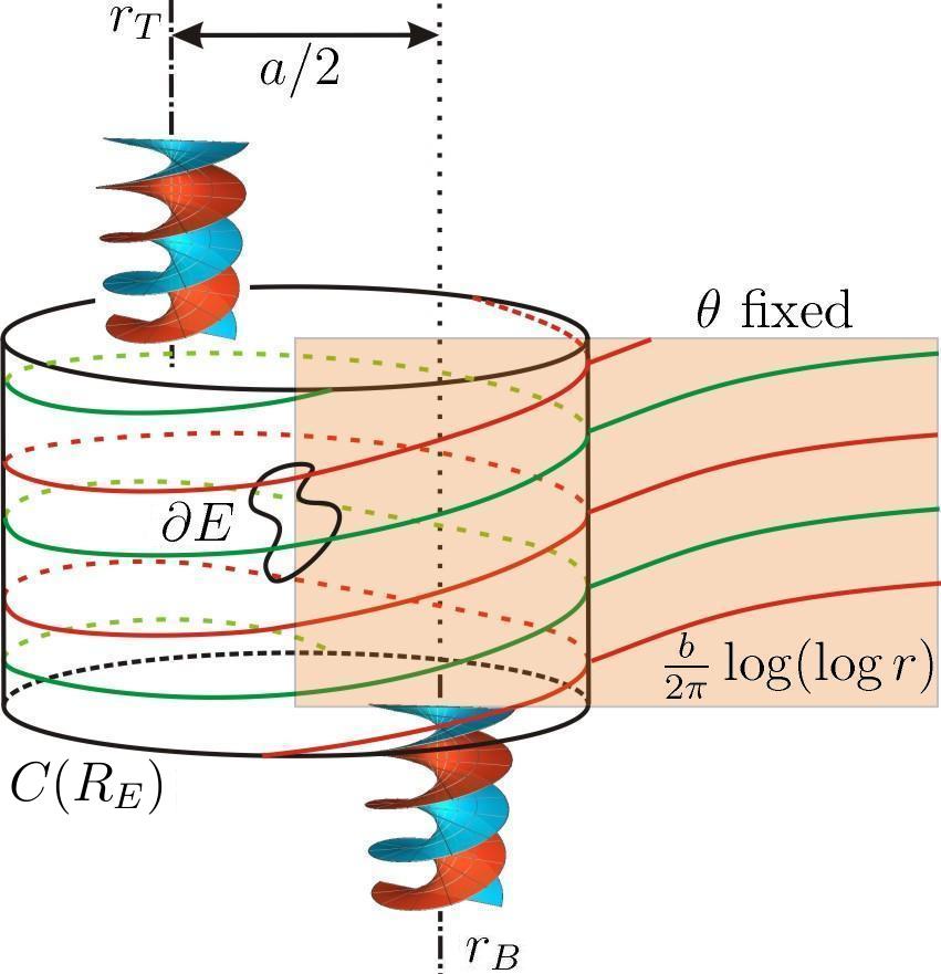
Figure 2: The embedded annulus $E$ with flux vector $(a,0,b)$ has the following description. Outside the cylinder $C(R_{E})$, $E$ consists of two horizontal multigraphs with asymptotic spacing $\pi$ between them. The translated surfaces $E+(0,0,-2\pi n-\frac{b}{2\pi}\log n)$ (resp. $E+(0,0,2\pi n-\frac{b}{2\pi}\log n)$) converge as $n\to\infty$ to a vertical helicoid $H_{T}$ (resp. $H_{B}$) such that $H_{B}=H_{T}+(0,a/2,0)$ (in the picture, $r_{T},r_{B}$ refer to the axes of these helicoids). The intersection of a vertical halfplane containing the $x_{3}$-axis with $E-C(R_{E})$ consists of an infinite number of curves, each of which is a graph of a function $u(r)$ that satisfies the property $\frac{u(r)}{\log(\log r)}$ converges to $\frac{b}{2\pi}$ as the radial distance $r$ to the $x_{3}$-axis tends to $\infty$.

Theorem 8.5 (Asymptotics of embedded minimal annular ends)

Given $a,b\geq 0$, there exist a positive number $R=R(a,b)$ and a properly embedded minimal annulus $E_{a,b}\subset\mathbb{R}^{3}$ with compact boundary and flux vector $(a,0,b)$ along its boundary, such that the following statements hold.

1. $E_{a,b}-C(R)$ consists of two disjoint multigraphs $\Sigma_{1},\Sigma_{2}$ over $D(\infty,R)$ of smooth functions $u_{1},u_{2}\colon\widetilde{D}(\infty,R)\to\mathbb{R}$ such that their gradients satisfy $\nabla u_{i}(r,\theta)\to 0$ as $r\to\infty$ and the separation function $w(r,\theta)=u_{1}(r,\theta)-u_{2}(r,\theta)$ between both multigraphs converges to $\pi$ as $r+|\theta|\to\infty$. Furthermore for ${\theta}$ fixed and $i=1,2$,

   $$\lim_{r\to\infty}\frac{u_{i}(r,\theta)}{\log(\log(r))}=\lim_{r\to\infty}\frac{u_{i}(r,\theta)}{\log(\log(r))}=\frac{b}{2\pi}.$$ (46)

2. The translated surfaces $E_{a,b}+(0,0,-2\pi n-\frac{b}{2\pi}\log n)$ (resp. $E_{a,b}+(0,0,2\pi n-\frac{b}{2\pi}\log n)$) converge as $n\to\infty$ to a vertical helicoid $H_{T}$ (resp. $H_{B}$) such that $H_{B}=H_{T}+(0,a/2,0)$. Note that this property together with item 1 imply that for different values of $a,b$, the related surfaces $E_{a,b}$ are not asymptotic after a rigid motion and homothety.

3. Every complete, embedded minimal annulus in $\mathbb{R}^{3}$ with compact boundary and infinite total curvature is asymptotic (up to a rigid motion and homothety) to exactly one of the surfaces $E_{a,b}$.

We will finish this section by reporting on the asymptotic behavior of any properly embedded minimal surface $M$ in $\mathbb{R}^{3}$ with finite genus and an infinite number of ends. We have already seen that such an $M$ has exactly two limit ends; it easily follows that each of its middle ends is asymptotic to a horizontal plane, after a fixed rotation of $M$. Also, after another rotation of $M$ around a vertical axis followed by a homothety, we can assume that the flux vector associated to its limit ends has the form $F=(h,0,1)$, where $h>0$. In this case $M$ is seen to be conformally a compact Riemann surface $\overline{M}$ punctured in a closed countable set with exactly two limit points corresponding to the two limit ends of $M$, and we can also describe the asymptotic behavior of the ends of $M$:

Theorem 8.6 (Asymptotic Limit End Property, Meeks, Pérez and Ros [64])

Let $M$ be a properly embedded minimal surface in $\mathbb{R}^{3}$ with finite genus $g$ and an infinite number of ends. Then, after a possible rotation and a homothety, the following statements hold.

1. $M$ has two limit ends. In fact, $M$ is conformally diffeomorphic to $\overline{M}-{\cal E}_{M}$, where $\overline{M}$ is a compact Riemann surface of genus $g$ and ${\cal E}_{M}=\{e_{n}\mid n\in\mathbb{Z}\}\cup\{e_{B},\,e_{T}\}$ is a countable closed subset of $\overline{M}$ with exactly two limit points $e_{T}$ and $e_{B}$. Furthermore, $\lim_{n\to-\infty}e_{n}=e_{B}$, $\lim_{n\to\infty}e_{n}=e_{T}$, and $e_{T}$ (resp. $e_{B}$) corresponds to the top (resp. bottom) end of $M$, while every $e_{n}$ with $n\in\mathbb{Z}$ corresponds to a middle end.

2. For each $n\in\mathbb{Z}$, there exists a punctured disk neighborhood $E_{n}\subset M\subset\overline{M}$ of $e_{n}$ which is asymptotic in $\mathbb{R}^{3}$ to a horizontal plane $P_{n}$ and which is a graph over its projection to $P_{n}$. Furthermore, the usual linear ordering on the index set $\mathbb{Z}$ respects the linear ordering of the heights of the related planes. The ordered set of heights $H=\{h_{n}=x_{3}(P_{n})\mid n\in\mathbb{Z}\}$ of these planes naturally corresponds to the set of heights of the middle ends of $M$.

3. There exists a positive constant $C_{M}$ such that if $|t|>C_{M}$, then the horizontal plane $\{x_{3}=t\}$ intersects $M$ in a proper arc when $t\in H$, or otherwise, $\{x_{3}=t\}$ intersects $M$ in a simple closed curve.

4. Let ${\eta}$ denote the unitary outward conormal along the boundary of $M_{t}=M\cap\{x_{3}\leq t\}$. Then the flux vector of $M$, which is defined to be

   $$F_{M}=\int_{\partial M_{t}}\eta\,ds$$

   (here $ds$ stands for the length element ), is independent of the choice of $t$ and has the form $F_{M}=(h,0,1)$, for some $h>0$.

5. Let $R_{h}\subset\mathbb{R}^{3}$ be the Riemann minimal example with horizontal tangent plane at infinity and flux vector $F=(h,0,1)$ along a compact horizontal section. Then, there exists a translation vector $v_{T}\in\mathbb{R}^{3}$ such that as $t\to\infty$, the function $d_{+}(t)=\sup\left\{\mbox{\rm dist}(p,{\cal R}_{h}+v_{T})\ |\ p\in M\cap\{x_{3}\geq t\}\right\}$ is finite and decays exponentially to zero. In a similar manner, there exists $v_{B}\in\mathbb{R}^{3}$ such that as $t\to-\infty$, the function $d_{-}(t)=\sup\left\{\mbox{\rm dist}(p,{\cal R}_{h}+v_{B})\ |\ p\in M\cap\{x_{3}\leq t\}\right\}$ is finite and decays exponentially to zero. Furthermore, $x_{2}(v_{T})=x_{2}(v_{B}).$

We now briefly outline the interesting elements of the proof of Theorem 8.6. The first important ingredient is that $M$ has bounded curvature and related uniform local area bounds in balls of fixed radius. Using these estimates and fixing an end representative $E_{T}$ of the top end of $M$, we can find a sequence of points $p_{n}\in M$ diverging on $E_{T}$ with Gaussian curvature bounded by above and away from zero. Our previous arguments show that a subsequence of the translated surfaces $M(n)=M-p_{n}$ converges as $n\to\infty$ to a translation of the Riemann minimal example $R_{h}$ whose flux vector is equal to $F_{M}=(h,0,1)$. Assume after a fixed translation of $M$ that the $M(n)$ converge to $R_{h}$. Similarly, for a bottom end representative $E_{B}$, we can find a divergent sequence of points $q_{n}$ such that the surfaces $M^{\prime}(n)=M-q_{n}$ converge to $R_{h}$ as $n\to\infty$.

The second key ingredient in the proof of the theorem is to use the non-zero Shiffman function $S_{E_{T}}$ of the end representative $E_{T}$, to prove that $M(n)$ converges exponentially quickly to $R_{h}$ as a function of the $x_{3}$-coordinate of the points $p_{n}$ (we are assuming here that the genus of $M$ is not zero, hence $S_{E_{T}}$ is not identically zero because $M$ is not a Riemann minimal example). This is done by first showing that the norm $|S_{E_{T}}|$ decays exponentially in terms of the $x_{3}$-coordinate function of $E_{T}$. In [64] we prove that the bounded Jacobi functions on $R_{h}$ are all linear and we then use this property to prove the related exponential decay of $|S_{E_{T}}|$. Once one has this exponential decay estimate for $|S_{E_{T}}|$, then elliptic theory can be used to show that $E_{T}$ converges exponentially quickly in terms of $x_{3}$-coordinates to $R_{h}+v_{T}$ for some vector $v_{T}\in\mathbb{R}^{3}$. Similarly, $E_{B}$ converges exponentially to $R_{h}+v_{B}$ for some $v_{B}\in\mathbb{R}^{3}$.

Finally, a forces argument using the Divergence Theorem applied to a certain Killing field on $\mathbb{R}^{3}$ shows that the $x_{2}$-coordinate of $v_{T}$ equals the $x_{2}$-coordinate of $v_{B}$, which completes our discussion on the proof of Theorem 8.6.

In conclusion, we remark on an important question for a possible generalization of the classification results discussed in this paper. This question asks whether or not a complete embedded minimal surface $M\subset\mathbb{R}^{3}$ of finite genus and compact boundary is always properly embedded. If this is the case, then we can replace in the statements of our theorems the phrase “finite genus, properly embedded minimal surfaces” by the phrase “finite genus, complete, embedded minimal surfaces”. As mentioned above, Colding and Minicozzi [21] have recently proved that this generalization holds when the surface has finite topology. Shortly afterwards, Meeks, Pérez and Ros [61] proved this result when the surface has finite genus and a countable number of ends; their result depends on the previously mentioned work in [21] and a related generalization by Meeks and Rosenberg [72] of the results in [21]. In relation to this problem, recall that Theorem 5.11 implies any properly embedded minimal surface has a countable number of ends. It remains open the outstanding question of whether or not a complete, embedded minimal surface of finite genus can have an uncountable number of ends.

William H. Meeks, III at bill@math.umass.edu
Mathematics Department, University of Massachusetts, Amherst, MA 01003 Joaquín Pérez at jperez@ugr.es
Department of Geometry and Topology, University of Granada, Granada, Spain

References

- [1] U. Abresch. Constant mean curvature tori in terms of elliptic functions. J. Reine Angew. Math., 374:169–192, 1987. MR0876223, Zbl 0597.53003.
- [2] A. Alarcón, L. Ferrer, and F. Martín. Density theorems for complete minimal surfaces in . Geom. Funct. Anal., 18(1):1–49, 2008. MR2399094, Zbl 1144.53013.
- [3] J. Bernstein and C. Breiner. Conformal structure of minimal surfaces with finite topology. Preprint available at http://arxiv.org/abs/0810.4478v1.
- [4] S. Bernstein. Uber ein geometrisches theorem und seine anwendung auf die partiellen differentialglechungen vom elliptischen typus. Math. Z., 26:551–558, 1927. MR1544873, Zbl JFM 53.0670.01.
- [5] A. Bobenko. All constant mean curvature tori in , , in terms of theta-functions. Math. Ann., 290(2):209–245, 1991.
- [6] O. Bonnet. Mémoire sur l’emploi d’un nouveau systeme de variables dans l’etude des surfaces courbes. J. Mathemém. p. appl., 2:153–266, 1860.
- [7] M. Callahan, D. Hoffman, and W. H. Meeks III. The structure of singly-periodic minimal surfaces. Invent. Math., 99:455–481, 1990. MR1032877, Zbl 695.53005.
- [8] E. Catalan. Sur les surfaces réglées dont l’aire est un minimum. J. Mathem. p. appl., 7:203–211, 1842.
- [9] T. H. Colding and W. P. Minicozzi II. The space of embedded minimal surfaces of fixed genus in a 3-manifold V; Fixed genus. Preprint math.DG/0509647 (2005).
- [10] T. H. Colding and W. P. Minicozzi II. Minimal surfaces, volume 4 of Courant Lecture Notes in Mathematics. New York University Courant Institute of Mathematical Sciences, New York, 1999. MR1683966, Zbl 0987.49025.
- [11] T. H. Colding and W. P. Minicozzi II. Complete properly embedded minimal surfaces in . Duke Math. J., 107:421–426, 2001. MR1823052, Zbl 1010.49025.
- [12] T. H. Colding and W. P. Minicozzi II. Embedded minimal disks: proper versus nonproper - global versus local. Transactions of the AMS, 356(1):283–289, 2003. MR2020033, Zbl 1046.53001.
- [13] T. H. Colding and W. P. Minicozzi II. Minimal disks that are double spiral staircases. Notices of the AMS, 50(3):327–339, 2003. MR1954009, Zbl pre02115046.
- [14] T. H. Colding and W. P. Minicozzi II. An excursion into geometric analysis. In Surveys of Differential Geometry IX - Eigenvalues of Laplacian and other geometric operators, pages 83–146. International Press, edited by Alexander Grigor’yan and Shing Tung Yau, 2004. MR2195407, Zbl 1076.53001.
- [15] T. H. Colding and W. P. Minicozzi II. The space of embedded minimal surfaces of fixed genus in a 3-manifold I; Estimates off the axis for disks. Ann. of Math., 160:27–68, 2004. MR2119717, Zbl 1070.53031.
- [16] T. H. Colding and W. P. Minicozzi II. The space of embedded minimal surfaces of fixed genus in a 3-manifold II; Multi-valued graphs in disks. Ann. of Math., 160:69–92, 2004. MR2119718, Zbl 1070.53032.
- [17] T. H. Colding and W. P. Minicozzi II. The space of embedded minimal surfaces of fixed genus in a 3-manifold III; Planar domains. Ann. of Math., 160:523–572, 2004. MR2123932, Zbl 1076.53068.
- [18] T. H. Colding and W. P. Minicozzi II. The space of embedded minimal surfaces of fixed genus in a 3-manifold IV; Locally simply-connected. Ann. of Math., 160:573–615, 2004. MR2123933, Zbl 1076.53069.
- [19] T. H. Colding and W. P. Minicozzi II. Embedded minimal disks. In Global theory of minimal surfaces, pages 405–438. American Mathematical Society, Providence, RI, for the Clay Mathematics Institute, Cambridge, MA, edited by D. Hoffman, 2005. MR2167253, Zbl 1078.53002.
- [20] T. H. Colding and W. P. Minicozzi II. Shapes of embedded minimal surfaces. Proc. National Academy of Sciences, 103:11106–11111, 2006. MR2242650, Zbl pre05272457.
- [21] T. H. Colding and W. P. Minicozzi II. The Calabi-Yau conjectures for embedded surfaces. Ann. of Math., 167:211–243, 2008. MR2373154, Zbl 1142.53012.
- [22] P. Collin. Topologie et courbure des surfaces minimales de . Ann. of Math. (2), 145–1:1–31, 1997. MR1432035, Zbl 886.53008.
- [23] P. Collin, R. Kusner, W. H. Meeks III, and H. Rosenberg. The geometry, conformal structure and topology of minimal surfaces with infinite topology. J. Differential Geom., 67:377–393, 2004. MR2153082, Zbl 1098.53006.
- [24] U. Dierkes, S. Hildebrandt, A. Küster, and O. Wohlrab. Minimal Surfaces I. Grundlehren der mathematischen Wissenschaften 295. Springer-Verlag, 1992. MR1215267, Zbl 0777.53012.
- [25] M. do Carmo and C. K. Peng. Stable complete minimal murfaces in are planes. Bulletin of the AMS, 1:903–906, 1979. MR0546314, Zbl 442.53013.
- [26] A. Douady and R. Douady. Changements de cadres á partir des surfaces minimales. Cahier de DIDIREM, 23(1), 1994. Edited by IREM de Paris7.
- [27] N. Ejiri and M. Kotani. Index and flat ends of minimal surfaces. Tokyo J. Math., 16(1):37–48, 1993. MR1223287, Zbl 0856.53013.
- [28] H. Federer. Geometric measure theory. Springer-Verlag, Berlin-Heidelberg, New York, 1969. MR0257325, Zbl 0176.00801.
- [29] L. Ferrer, F. Martín, and W. H. Meeks III. The existence of proper minimal surfaces of arbitrary topological type. Preprint.
- [30] D. Fischer-Colbrie and R. Schoen. The structure of complete stable minimal surfaces in 3-manifolds of non-negative scalar curvature. Comm. on Pure and Appl. Math., 33:199–211, 1980. MR0562550, Zbl 439.53060.
- [31] C. Frohman. The topological uniqueness of triply-periodic minimal surfaces in . J. Differential Geom., 31:277–283, 1990. MR1030674, Zbl 0689.53002.
- [32] C. Frohman and W. H. Meeks III. The topology of complete one-ended minimal surfaces and Heegaard surfaces in . Bulletin of the AMS, 23(2):417–421, 1990.
- [33] C. Frohman and W. H. Meeks III. The ordering theorem for the ends of properly embedded minimal surfaces. Topology, 36(3):605–617, 1997. MR1422427, Zbl 878.53008.
- [34] C. Frohman and W. H. Meeks III. The topological uniqueness of complete one-ended minimal surfaces and Heegaard surfaces in . J. Amer. Math. Soc., 10(3):495–512, 1997. MR1443545, Zbl 0886.57015.
- [35] C. Frohman and W. H. Meeks III. The topological uniqueness of complete one-ended minimal surfaces and heegaard surfaces in . J. Amer. Math. Soc., 10(3):495–512, 1997. MR1443545, Zbl 0886.57015.
- [36] C. Frohman and W. H. Meeks III. The topological classification of minimal surfaces in . MR2415385, 2008.
- [37] F. Gesztesy and R. Weikard. Elliptic algebro-geometric solutions of the KdV and AKNS hierarchies—an analytic approach. Bull. Amer. Math. Soc. (N.S.), 35(4):271–317, 1998. MR1638298 (99i:58075).
- [38] P. Griffiths and J. Harris. Principles of Algebraic Geometry. (Pure and Applied Mathematics). Wiley-Interscience, 1978. MR0507725, Zbl 408.14001.
- [39] A. Grigor’yan, Y. Netrusov, and S. T. Yau. Eigenvalues of elliptic operators and geometric applications. In Surveys of Differential Geometry IX, pages 147–218. International Press, 2004. MR2195408, Zbl 1061.58027.
- [40] L. Hauswirth, J. Pérez, and P. Romon. Embedded minimal ends of finite type. Transactions of the AMS, 353:1335–1370, 2001. MR1806738, Zbl 0986.53005.
- [41] D. Hoffman and W. H. Meeks III. The strong halfspace theorem for minimal surfaces. Invent. Math., 101:373–377, 1990. MR1062966, Zbl 722.53054.
- [42] A. Huber. On subharmonic functions and differential geometry in the large. Comment. Math. Helvetici, 32:181–206, 1957. MR0094452, Zbl 0080.15001.
- [43] L. Jorge and W. H. Meeks III. The topology of complete minimal surfaces of finite total Gaussian curvature. Topology, 22(2):203–221, 1983. MR0683761, Zbl 0517.53008.
- [44] N. Joshi. The second Painlevé hierarchy and the stationary KdV hierarchy. Publ. Res. Inst. Math. Sci., 40(3):1039–1061, 2004. MR2074710, Zbl 1063.33030.
- [45] M. Kilian and U. Schmidt. In the moduli of constant mean curvatrure cylinders of finite type in the 3-sphere. Preprint arXiv:math.DG/0712.0108v1.
- [46] N. Korevaar, R. Kusner, and B. Solomon. The structure of complete embedded surfaces with constant mean curvature. J. Differential Geom., 30:465–503, 1989. MR1010168, Zbl 0726.53007.
- [47] P. Li and J. Wang. Finiteness of disjoint minimal graphs. Math. Research Letters, 8(6):771–777, 2001. MR1879819, Zbl 0999.05055.
- [48] R. B. Lockhart and R. C. McOwen. Elliptic differential operators on noncompact manifolds. Ann. Scuola Norm. Sup. Pisa, 12(3):409–447, 1985. MR0837256, Zbl 0615.58048.
- [49] F. J. López and A. Ros. On embedded complete minimal surfaces of genus zero. J. Differential Geom., 33(1):293–300, 1991. MR1085145, Zbl 719.53004.
- [50] F. Martin, W. H. Meeks III, and N. Nadirashvili. Bounded domains which are universal for minimal surfaces. American Journal of Math., 129(2):455–461, 2007. MR2306042, Zbl pre05152573.
- [51] F. Martin and S. Morales. On the asymptotic behavior of a complete bounded minimal surface in . Transactions of the AMS, 356(10):3985–3994, 2004. MR2058515, Zbl 1057.53009.
- [52] F. Martin and S. Morales. Complete proper minimal surfaces in convex bodies of . Duke Math. J., 128(3):559–593, 2005. MR2145744, Zbl 1082.53009.
- [53] F. Martin and N. Nadirashvili. A Jordan curve spanned by a complete minimal surface. Arch. Ration. Mech. Anal., 184(2):285–301, 2007. MR2299764, Zbl 1114.49039.
- [54] W. H. Meeks III. A survey of the geometric results in the classical theory of minimal surfaces. Bol. Soc. Brasil Mat., 12:29–86, 1981. MR0671473, Zbl 0577.53007.
- [55] W. H. Meeks III. The geometry, topology, and existence of periodic minimal surfaces. Proceedings of Symposia in Pure Math., 54:333–374, 1993. Part I. MR1216594, Zbl 812.49030.
- [56] W. H. Meeks III. The regularity of the singular set in the Colding and Minicozzi lamination theorem. Duke Math. J., 123(2):329–334, 2004. MR2066941, Zbl pre02127998.
- [57] W. H. Meeks III and J. Pérez. The classical theory of minimal surfaces. Preprint, available at http://www.ugr.es/local/jperez/papers/papers.htm.
- [58] W. H. Meeks III and J. Pérez. Embedded minimal surfaces of finite topology. Preprint, available at http://www.ugr.es/local/jperez/papers/papers.htm.
- [59] W. H. Meeks III and J. Pérez. Finite type annular ends for harmonic functions. Preprint, available at http://www.ugr.es/local/jperez/papers/papers.htm.
- [60] W. H. Meeks III and J. Pérez. Conformal properties in classical minimal surface theory. In Surveys of Differential Geometry IX - Eigenvalues of Laplacian and other geometric operators, pages 275–336. International Press, edited by Alexander Grigor’yan and Shing Tung Yau, 2004. MR2195411, Zbl 1086.53007.
- [61] W. H. Meeks III, J. Pérez, and A. Ros. The embedded Calabi-Yau conjectures for finite genus. Preprint, available at http://www.ugr.es/local/jperez/papers/papers.htm.
- [62] W. H. Meeks III, J. Pérez, and A. Ros. Limit leaves of a CMC lamination are stable. To appear in J. Differential Geometry, available at arXiv:0801.4345 and at http://www.ugr.es/local/jperez/papers/papers.htm.
- [63] W. H. Meeks III, J. Pérez, and A. Ros. Local removable singularity theorems for minimal and -laminations. Preprint, available at http://www.ugr.es/local/jperez/papers/papers.htm.
- [64] W. H. Meeks III, J. Pérez, and A. Ros. Properly embedded minimal planar domains. Preprint, available at http://www.ugr.es/local/jperez/papers/papers.htm.
- [65] W. H. Meeks III, J. Pérez, and A. Ros. Structure theorems for singular minimal laminations. Preprint, available at http://www.ugr.es/local/jperez/papers/papers.htm.
- [66] W. H. Meeks III, J. Pérez, and A. Ros. Uniqueness of the Riemann minimal examples. Invent. Math., 133:107–132, 1998. MR1626477, Zbl 916.53004.
- [67] W. H. Meeks III, J. Pérez, and A. Ros. The geometry of minimal surfaces of finite genus I; curvature estimates and quasiperiodicity. J. Differential Geom., 66:1–45, 2004. MR2128712, Zbl 1068.53012.
- [68] W. H. Meeks III, J. Pérez, and A. Ros. The geometry of minimal surfaces of finite genus II; nonexistence of one limit end examples. Invent. Math., 158:323–341, 2004. MR2096796, Zbl 1070.53003.
- [69] W. H. Meeks III, J. Pérez, and A. Ros. Stable constant mean curvature surfaces. In Handbook of Geometrical Analysis, volume 1, pages 301–380. International Press, edited by Lizhen Ji, Peter Li, Richard Schoen and Leon Simon, ISBN: 978-1-57146-130-8, 2008. MR2483369, Zbl 1154.53009.
- [70] W. H. Meeks III and H. Rosenberg. The geometry and conformal structure of properly embedded minimal surfaces of finite topology in . Invent. Math., 114:625–639, 1993. MR1244914, Zbl 0803.53007.
- [71] W. H. Meeks III and H. Rosenberg. The uniqueness of the helicoid. Ann. of Math., 161:723–754, 2005. MR2153399, Zbl 1102.53005.
- [72] W. H. Meeks III and H. Rosenberg. The minimal lamination closure theorem. Duke Math. Journal, 133(3):467––497, 2006. MR2228460, Zbl 1098.53007.
- [73] W. H. Meeks III and H. Rosenberg. Maximum principles at infinity. J. Differential Geometry, 79(1):141–165, 2008. MR2401421, Zbl pre05285650.
- [74] W. H. Meeks III, L. Simon, and S. T. Yau. The existence of embedded minimal surfaces, exotic spheres and positive Ricci curvature. Ann. of Math., 116:221–259, 1982. MR0678484, Zbl 0521.53007.
- [75] W. H. Meeks III and S. T. Yau. The classical Plateau problem and the topology of three-dimensional manifolds. Topology, 21(4):409–442, 1982. MR0670745, Zbl 0489.57002.
- [76] W. H. Meeks III and S. T. Yau. The existence of embedded minimal surfaces and the problem of uniqueness. Math. Z., 179:151–168, 1982. MR0645492, Zbl 0479.49026.
- [77] S. Montiel and A. Ros. Schrödinger operators associated to a holomorphic map. In Global Differential Geometry and Global Analysis (Berlin, 1990), volume 1481 of Lecture Notes in Mathematics, pages 147–174. Springer-Verlag, 1991. MR1178529, Zbl 744.58007.
- [78] C. B. Morrey. The problem of Plateau on a Riemannian manifold. Ann. of Math., 49:807–851, 1948. MR0027137, Zbl 0033.39601.
- [79] N. Nadirashvili. Hadamard’s and Calabi-Yau’s conjectures on negatively curved and minimal surfaces. Invent. Math., 126(3):457–465, 1996. MR1419004, Zbl 0881.53053.
- [80] R. Osserman. Global properties of minimal surfaces in and . Ann. of Math., 80(2):340–364, 1964. MR0179701, Zbl 0134.38502.
- [81] R. Osserman. A Survey of Minimal Surfaces. Dover Publications, New York, 2nd edition, 1986. MR0852409, Zbl 0209.52901.
- [82] R. Osserman and M. Schiffer. Doubly-connected minimal surfaces. Arch. Rat. Mech. Anal., 58:285–307, 1975.
- [83] J. Pérez. On singly-periodic minimal surfaces with planar ends. Transactions of the AMS, 6:2371–2389, 1997. MR1407709, Zbl 882.53007.
- [84] J. Pérez and A. Ros. Properly embedded minimal surfaces with finite total curvature. In The Global Theory of Minimal Surfaces in Flat Spaces, pages 15–66. Lecture Notes in Math 1775, Springer-Verlag, 2002. G. P. Pirola, editor. MR1901613, Zbl 1028.53005.
- [85] U. Pinkall and I. Sterling. On the classification of constant mean curvature tori. Ann. of Math., 130:407–451, 1989. MR1014929, Zbl 0683.53053.
- [86] A. V. Pogorelov. On the stability of minimal surfaces. Soviet Math. Dokl., 24:274–276, 1981. MR0630142, Zbl 0495.53005.
- [87] B. Riemann. Über die Fläche vom kleinsten Inhalt bei gegebener Begrenzung. Abh. Königl, d. Wiss. Göttingen, Mathem. Cl., 13:3–52, 1867. K. Hattendorf, editor. JFM 01.0218.01.
- [88] B. Riemann. Ouevres Mathématiques de Riemann. Gauthiers-Villars, Paris, 1898.
- [89] A. Ros. One-sided complete stable minimal surfaces. Journal Differential Geometry, 74:69–92, 2006. MR2260928, Zbl 1110.53009.
- [90] R. Schoen. Estimates for Stable Minimal Surfaces in Three Dimensional Manifolds, volume 103 of Ann. of Math. Studies. Princeton University Press, 1983. MR0795231, Zbl 532.53042.
- [91] R. Schoen. Uniqueness, symmetry, and embeddedness of minimal surfaces. J. Differential Geom., 18:791–809, 1983. MR0730928, Zbl 0575.53037.
- [92] G. Segal and G. Wilson. Loop groups and equations of type. Pub. Math. de I.H.E.S., 61:5–65, 1985. MR0783348, Zbl 0592.35112.
- [93] M. Shiffman. On surfaces of stationary area bounded by two circles, or convex curves, in parallel planes. Ann. of Math., 63:77–90, 1956. MR0074695, Zbl 0070.16803.
- [94] L. Simon. Lectures on geometric measure theory. In Proceedings of the Center for Mathematical Analysis, volume 3, Canberra, Australia, 1983. Australian National University. MR0756417, Zbl 546.49019.
- [95] V. G. Tkachev. Disjoint minimal graphs. Annals of Global Analysis and Geometry, 35(2):139–155, 2009.
- [96] R. Weikard. On rational and periodic solutions of stationary KdV equations. Doc. Math., 4:107–126 (electronic), 1999. MR1683290, Zbl 0972.35121.