Enhanced heavy quark-pair production in strong SU(2) color field

Abstract

Non-perturbative charm and bottom quark-pair production is investigated in the early stage of heavy ion collisions. Following our earlier works, the time-dependent study is based on a kinetic description of fermion-pair production in strong non-Abelian fields. We introduce time-dependent chromo-electric external field with a pulse-like time evolution, which simulates the overlap of two colliding heavy ions. The calculations is performed in a SU(2) color model with finite current quark masses. Yields of heavy quark-pairs are compared to the ones of light and strange quark-pairs. We show that the small inverse duration time of the field pulse determines the efficiency of the quark-pair production. Thus we do not see the expected suppression for heavy quark production, as follows from the Schwinger formula for constant field, but rather an enhanced heavy quark production at ultrarelativistic energies. We convert pulse duration time-dependent results into collisional energy dependence and introduce flavour-dependent energy string tensions, which can be used in string based model calculations at RHIC and LHC energies.

I Introduction

The main aim of ultrarelativistic heavy ion collisions is to create extreme high energy densities and study the deconfinement phase transition of colored quarks and gluons. Experiments at the BNL Relativistic Heavy Ion Collider (RHIC) have been investigated the center of mass colliding region up to $\sqrt{s}=200$ AGeV and detectors at CERN Large Hadronic Collider (LHC) are ready to explore the energy range to $\sqrt{s}=5500$ AGeV. At such high energies the colliding nuclei are two colliding sheets of nucleons with a huge Lorentz-contraction ($\gamma_{cm}=100$ at RHIC and $\gamma_{cm}=2750$ at LHC), surrounded by a gluon cloud. Their overlap results in a strong chromo-electric and chromo-magnetic field to be built up. Particles, namely gluons and quark-antiquark pairs are produced from this strong field, similarly to the Schwinger mechanism in quantum electrodynamics (QED) schw51 . The particle production rate depends on the field strength, which is varying in time. The soft particles produced in such a non-perturbative way form the bulk of the wanted quark-gluon plasma, after they successfully thermalized. Light and strange quarks loose most of their original properties during thermalization, but charm and bottom quarks conserve certain characteristic properties, which can be studied after the whole evolution of the heavy ion collisions. In this paper we investigate the primordial non-perturbative production of heavy charm and bottom quarks, and explore the early stage of heavy ion collisions.

Recently the study of heavy quark production has received wide interest, because open charm has been measured at RHIC in d+Au Adams:2004fc , Cu+Cu Baumgart:2008xe , and Au+Au Abelev:2008hja collisions. The STAR Adams:2004fc ; Baumgart:2008xe ; Abelev:2008hja and PHENIX Adare:2006hc ; Adare:2006nq experiments have obtained different results (within a factor of 3), which finding opened vivid experimental and theoretical discussions QM08 . A review on heavy-flavour production has been published recently Frawley:2008kk . Theoretical calculations based on perturbative quantum chromodynamics (pQCD) at fixed order next to-leading logaritms (FONLL) have found that the measured total charm cross section only comparable with the upper limit of the FONLL calculations. Thus there is a room for non-perturbative production channels. However, the situation is very complex, as it was discussed in a recent paper Pop:2009sd : measured heavy quark radiative and collisional energy loss in heavy ion collisions must fit into the picture, as well as the regeneration of charm hadrons in quark coalescence channels. The interest on this question supports the importance of our investigation of primordial non-perturbative heavy quark production.

Theoretical descriptions of particle production in high energy $pp$ collisions are based on the introduction of chromoelectric flux tube (’string’) models FRITIOF ; HIJ ; RQMD ; QGSM ; HIJINGBB . String picture is a good example of how to convert the kinetic energy of a collision into field energy, than later on gain the stored kinetic energy back. However, at RHIC and LHC energies the string density is expected to be so large that a strong collective gluon field will be formed in the whole available transverse volume. Furthermore, the gluon number will be so high that a classical gluon field as the expectation value of the quantum field can be considered in the reaction volume Gyul97 ; Magas2002 ; Topor05 . Alternatively at extremely high energies, nucleus nucleus collisions can be described as two colliding sheets of Colored Glass Condensate. In the framework of this model it was shown that in the early stage of collision longitudinal color-electric and color-magnetic fields are created Lappi:2006fp . The properties of such non-Abelian classical fields and details of gluon production were studied very intensively during the last years, especially asymptotic solutions (for summaries see Refs. McLerran:2001sr ; IanVen03 ). Fermion production was calculated recently Gelis:2006yv ; Gelis:2006cr ; Blaizot:2004wv .

Fermion pair production together with boson pair production were investigated by different models of particle production from strong Abelian Gatoff87 ; Kluger91 ; Gatoff92 ; Wong95 ; Eisenberg95 ; Vin02 ; Per03 ; Prozorkevich:2004yp ; Pervushin:2006vh ; Mihaila:2009ge ; Dawson:2009cn and non-Abelian Prozor03 ; Diet03 ; HeinzOchs fields. These calculations concentrated mostly on the bulk properties of the gluon and quark matter, the time evolution of the system, the time dependence of energy and particle number densities, and the appearance of fast thermalization.

In our previous papers (see Ref. SkokLev05 ; SkokLev07 ) we investigated massless fermion and boson production in strong Abelian and non-Abelian external electric field. During these calculations we have realized, that the role of mass becomes unimportant when the collisional energy is increasing and the the pulse duration time becomes comparable to the inverse quark mass Levai:2008wf . In this paper we describe strange, charm, and bottom quark-pair production. Motivated by the problems raised in Ref. Pop:2009sd we investigate the role of string tension in the Schwinger mechanism for heavy quark pair production.

The energy dependece of the string tension was investigated earlier Magas2002 . Instead of the usual $\kappa\sim 1$ GeV/fm value the much higher effective string tension, $\kappa\sim 5-12$ GeV/fm appeared in the calculations. This open question motivates our investigation also.

In this paper we solve the kinetic model in the presence of an external SU(2) non-Abelian color field. We focus on particle production with finite mass at different duration time of the quickly changing external field. Section 2 summarizes theoretical background of the kinetic equation for color Wigner function. In Section 3 we consider the kinetic equation for pure longitudinal time-dependent SU(2) color field, which will be solved numerically. In Section 4 we summarize and discuss our numerical results from general point of view. We discuss the collision energy and pulse duration time-dependence of heavy quark production. In a phenomenological way we introduce flavour specific string tensions to connect our numerical results and Schwinger estimate.

In Appendix A we derive general kinetic equation for the Wigner function starting from QCD Lagrangian. In Appendix B we show exact solution of the kinetic equation for SU(2) color case, that supports our numerical calculation.

II The kinetic equation for the Wigner function

The equation of motion for color Wigner function $W(\mathbf{k},t)$ in the gradient approximation reads (see Appendix A for details)

$$\partial_{t}W+\frac{g}{8}\frac{\partial}{\partial k_{i}}\left(4\{W,F_{0i}\}+\right.$$

$$\left.+2\left\{F_{i\nu},[W,\gamma^{0}\gamma^{\nu}]\right\}-\left[F_{i\nu},\{W,\gamma^{0}\gamma^{\nu}\}\right]\right)=$$

$$=ik_{i}\{\gamma^{0}\gamma^{i},W\}-im[\gamma^{0},W]+ig\left[A_{i}\,,[\gamma^{0}\gamma^{i},W]\right].\ \ \$$ (1)

Here $m$ denotes the current mass of the fermions, $g$ is the coupling constant, $A_{\mu}$ is the 4-potential of an external space-homogeneous color field and $F_{\mu\nu}$ is corresponding field tensor

$$F_{\mu\nu}=\partial_{\mu}A_{\nu}-\partial_{\nu}A_{\mu}-ig[A_{\mu},A_{\nu}].$$ (2)

The validity of gradient approximation requires that the Wigner function is sufficiently smooth in momentum space and the field strength varies slowly in coordinate space. The corresponding characteristic lengths must satisfy the following relation $(\Delta p)_{W}(\Delta x)_{F}\gg 1$, where $(\Delta p)_{W}$ is connected to the momentum gradients of the Wigner function and $(\Delta x)_{F}$ to space gradients of the field.

The color decomposition of the Wigner function with SU($N_{c}$) generators in the fundamental representation is given by

$$W=W^{s}+W^{a}t^{a},\,\,\ \ \ a=1,2,...,N_{c}^{2}-1\ ,$$ (3)

where $W^{s}$ is the color singlet part and $W^{a}$ is the color multiplet components. It is also convenient to perform spinor decomposition separating scalar $a$, vector $b_{\mu}$, tensor $c_{\mu\nu}$, axial vector $d_{\mu}$ and pseudo-scalar parts $e$:

$$W^{s|a}=a^{s|a}+b^{s|a}_{\mu}\gamma^{\mu}+c^{s|a}_{\mu\nu}\sigma^{\mu\nu}+d^{s|a}_{\mu}\gamma^{\mu}\gamma^{5}+ie^{s|a}\gamma^{5}.$$ (4)

The asymmetric tensor components of the Wigner function is convenient to decompose into axial and polar vectors $c_{1}^{j}=c^{j0}$ and $c_{2}^{j}=\frac{1}{2}\epsilon^{0\omega\rho j}c_{\omega\rho}$ correspondingly.

III Kinetic equation in SU(2) with color isotropic external field

After the color and spinor decomposition of the equations for the Wigner function in case of pure longitudinal external SU(2) color field with fixed color direction $A^{a}_{z}=A^{\diamond}_{z}n^{a}$, where $n^{a}n^{a}=3$ and $\partial_{t}n^{a}=0$ SkokLev07 , we obtain the following system of equations for the singlet component

$$\partial_{t}a^{s}+\frac{3g}{4}E^{\diamond}_{z}\frac{\partial}{\partial k_{z}}a^{\diamond}=-4\mathbf{k}\mathbf{c}_{1}^{s},$$ (5)

$$\partial_{t}e^{s}+\frac{3g}{4}E^{\diamond}_{z}\frac{\partial}{\partial k_{z}}e^{\diamond}=-4\mathbf{k}\mathbf{c}_{2}^{s}-2md^{s}_{0},$$ (6)

$$\partial_{t}b^{s}_{0}+\frac{3g}{4}E^{\diamond}_{z}\frac{\partial}{\partial k_{z}}b^{\diamond}_{0}=0,$$ (7)

$$\partial_{t}\mathbf{b}^{s}+\frac{3g}{4}E^{\diamond}_{z}\frac{\partial}{\partial k_{z}}\mathbf{b}^{\diamond}=2[\mathbf{k}\times\mathbf{d}^{s}]+4m\mathbf{c}_{1}^{s},$$ (8)

$$\partial_{t}d^{s}_{0}+\frac{3g}{4}E^{\diamond}_{z}\frac{\partial}{\partial k_{z}}d^{\diamond}_{0}=2me^{s},$$ (9)

$$\partial_{t}\mathbf{d}^{s}+\frac{3g}{4}E^{\diamond}_{z}\frac{\partial}{\partial k_{z}}\mathbf{d}^{\diamond}=2[\mathbf{k}\times\mathbf{b^{s}}],$$ (10)

$$\partial_{t}\mathbf{c}_{1}^{s}+\frac{3g}{4}E^{\diamond}_{z}\frac{\partial}{\partial k_{z}}\mathbf{c}_{1}^{\diamond}=a^{s}\mathbf{k}-m\mathbf{b}^{s},$$ (11)

$$\partial_{t}\mathbf{c}_{2}^{s}+\frac{3g}{4}E^{\diamond}_{z}\frac{\partial}{\partial k_{z}}\mathbf{c}_{2}^{\diamond}=e^{s}\mathbf{k};$$ (12)

and the triplet components

$$\partial_{t}a^{\diamond}+gE^{\diamond}_{z}\frac{\partial}{\partial k_{z}}a^{s}=-4\mathbf{k}\mathbf{c}_{1}^{\diamond},$$ (13)

$$\partial_{t}e^{\diamond}+gE^{\diamond}_{z}\frac{\partial}{\partial k_{z}}e^{s}=-4\mathbf{k}\mathbf{c}_{2}^{\diamond}-2md^{\diamond}_{0},$$ (14)

$$\partial_{t}b^{\diamond}_{0}+gE^{\diamond}_{z}\frac{\partial}{\partial k_{z}}b^{s}_{0}=0,$$ (15)

$$\partial_{t}\mathbf{b}^{\diamond}+gE^{\diamond}_{z}\frac{\partial}{\partial k_{z}}\mathbf{b}^{s}=2[\mathbf{k}\times\mathbf{d}^{\diamond}]+4m\mathbf{c}_{1}^{\diamond},$$ (16)

$$\partial_{t}d^{\diamond}_{0}+gE^{\diamond}_{z}\frac{\partial}{\partial k_{z}}d^{s}_{0}\delta^{bc}=2me^{\diamond},$$ (17)

$$\partial_{t}\mathbf{d}^{\diamond}+gE^{\diamond}_{z}\frac{\partial}{\partial k_{z}}\mathbf{d}^{s}=2[\mathbf{k}\times\mathbf{b}^{\diamond}],$$ (18)

$$\partial_{t}\mathbf{c}_{1}^{\diamond}+gE^{\diamond}_{z}\frac{\partial}{\partial k_{z}}\mathbf{c}_{1}^{s}=a^{\diamond}\mathbf{k}-m\mathbf{b}^{\diamond},$$ (19)

$$\partial_{t}\mathbf{c}_{2}^{\diamond}+gE^{\diamond}_{z}\frac{\partial}{\partial k_{z}}\mathbf{c}_{2}^{s}=e^{c}\mathbf{k}.$$ (20)

The distribution function for massive fermions is completely defined by components ${a,b}$ SkokLev07 :

$$f_{q}(\mathbf{k},t)=\frac{ma^{s}(\mathbf{k},t)+\mathbf{k}\,\mathbf{b}^{s}(\mathbf{k},t)}{\omega(\mathbf{k})}+\frac{1}{2},$$ (21)

where ${\omega(\mathbf{k})}=\sqrt{\mathbf{k}^{2}+m^{2}}$. Thus for time- and momentum-dependent distribution functions scalar $a$, vector $b_{\mu}$, axial vector $d_{\mu}$, and tensor $c$ components of the Wigner function are needed, only.

The initial conditions for the Wigner function in vacuum reads (see Appendix A)

$$a^{s} = -\frac{1}{2}\frac{m}{\omega},$$ (22)

$$\mathbf{b}^{s} = -\frac{1}{2}\frac{\mathbf{k}}{\omega}.$$ (23)

Considering vacuum initial condition symmetry we obtain the following equations for the singlet (we redefined $\mathbf{c}=\mathbf{c}_{1}$ to simplify reading)

$$\partial_{t}a^{s}+\frac{3g}{4}E^{\diamond}_{z}\frac{\partial}{\partial k_{z}}a^{\diamond}=-4(k_{z}c_{z}^{s}+k_{\perp}c_{\perp}^{s}),$$ (24)

$$\partial_{t}b_{z}^{s}+\frac{3g}{4}E^{\diamond}_{z}\frac{\partial}{\partial k_{z}}b_{z}^{\diamond}=2k_{\perp}d_{x}^{s}+4mc_{z}^{s},$$ (25)

$$\partial_{t}b_{\perp}^{s}+\frac{3g}{4}E^{\diamond}_{z}\frac{\partial}{\partial k_{z}}b_{\perp}^{\diamond}=-2k_{z}d_{x}^{s}+4mc_{\perp}^{s},$$ (26)

$$\partial_{t}d_{x}^{s}+\frac{3g}{4}E^{\diamond}_{z}\frac{\partial}{\partial k_{z}}d_{x}^{\diamond}=2(k_{z}b_{\perp}^{s}-k_{\perp}b_{z}^{s}),$$ (27)

$$\partial_{t}c_{z}^{s}+\frac{3g}{4}E^{\diamond}_{z}\frac{\partial}{\partial k_{z}}c_{z}^{\diamond}=a^{s}k_{z}-mb_{z}^{s},$$ (28)

$$\partial_{t}c_{\perp}^{s}+\frac{3g}{4}E^{\diamond}_{z}\frac{\partial}{\partial k_{z}}c_{\perp}^{\diamond}=a^{s}k_{\perp}-mb_{\perp}^{s}\ ;$$ (29)

and for the triplet components

$$\partial_{t}a^{\diamond}+gE^{\diamond}_{z}\frac{\partial}{\partial k_{z}}a^{s}=-4(k_{z}c_{z}^{\diamond}+k_{\perp}c_{\perp}^{\diamond}),$$ (30)

$$\partial_{t}b_{z}^{\diamond}+gE^{\diamond}_{z}\frac{\partial}{\partial k_{z}}b_{z}^{s}=2k_{\perp}d_{x}^{\diamond}+4mc_{z}^{\diamond},$$ (31)

$$\partial_{t}b_{\perp}^{\diamond}+gE^{\diamond}_{z}\frac{\partial}{\partial k_{z}}b_{\perp}^{s}=-2k_{z}d_{x}^{\diamond}+4mc_{\perp}^{\diamond},$$ (32)

$$\partial_{t}d_{x}^{\diamond}+gE^{\diamond}_{z}\frac{\partial}{\partial k_{z}}d_{x}^{s}=2(k_{z}b_{\perp}^{\diamond}-k_{\perp}b_{z}^{\diamond}),$$ (33)

$$\partial_{t}c_{z}^{\diamond}+gE^{\diamond}_{z}\frac{\partial}{\partial k_{z}}c_{z}^{s}=a^{\diamond}k_{z}-mb_{z}^{\diamond},$$ (34)

$$\partial_{t}c_{\perp}^{\diamond}+gE^{\diamond}_{z}\frac{\partial}{\partial k_{z}}c_{\perp}^{s}=a^{\diamond}k_{\perp}-mb_{\perp}^{\diamond}\ ;$$ (35)

where we introduced the following vector decomposition

$$\mathbf{v}=v_{z}\mathbf{n}+v_{\perp}\frac{\mathbf{k}_{\perp}}{k_{\perp}}+v_{x}\left[\mathbf{n}\times\frac{\mathbf{k}_{\perp}}{k_{\perp}}\right]\ .$$ (36)

Here the unit vector collinear to the field direction, $\mathbf{n}$, is given by $\mathbf{n}=\mathbf{E}^{\diamond}/|\mathbf{E}^{\diamond}|=(0,0,1)$ and $\mathbf{k}_{\perp}=(k_{1},k_{2},0)$. As follows from Eqs. (24-35), the axial part of vector $b_{x}$, tensor components $c_{x}$, longitudinal $d_{z}$ and perpendicular $d_{\perp}$ parts of axial vector components do not contribute to the evolution of the distribution function.

These equations could be further simplified and transformed to ones that are similar to Abelian case (see Appendix B for details).

IV Numerical results and discussions

IV.1 General results

In Ref. SkokLev07 we have solved the above equations for massless (light) quarks and described their longitudinal and transverse momentum distributions. Here we focus on the integrated particle yields and discuss the obtained results, focusing on massive (heavy) quark production.

In the numerical calculation we have used the following parameters: the maximal magnitude of the field $E_{0}=0.68$ GeV/fm; the strong coupling constant $g=2$; the current quark masses $m_{u,d}=8$ MeV, $m_{s}=150$ MeV, $m_{c}=1.2$ GeV, $m_{b}=4.2$ GeV for light, strange, charm and bottom quarks, correspondingly. The value of maximal magnitude of the field corresponds to the effective string tension $\kappa\sim 1.17$ GeV/fm. The reason why we use this value will be explained below, in Subsection IV.2.

The particle production is ignited by a pulse-like color field simulating a heavy ion collision SkokLev07 :

$$E^{\diamond}(t)=E_{0}\cdot\left[1-\textrm{tanh}^{2}(t/\tau)\right],$$ (37)

where $\tau$ is a pulse duration time.

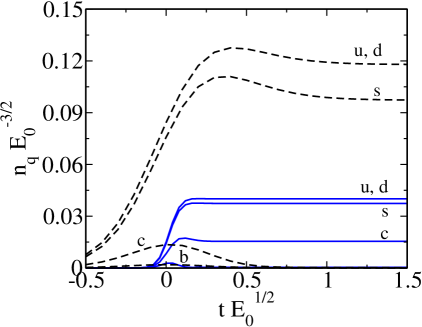
Figure 1: The dimensionless quark number density for different flavours, $n_{q}(t)E_{0}^{-3/2}$, as a function of dimensionless time $tE_{0}^{1/2}$ for different pulse duration, $\tau E_{0}^{1/2}=0.1$ (solid lines) and $\tau E_{0}^{1/2}=0.5$ (dashed lines).

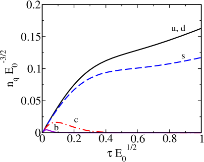
Figure 2: The dimensionless quark number densities at the asymptotic final state, $n_{q}(t\gg\tau)E_{0}^{-3/2}$, as a function of pulse duration time $\tau E_{0}^{1/2}$.

The suppression factor of heavier quark $Q$ to light one $u$ is defined in the asymptotic future (c.f.  schw51 ), $t\gg\tau$, as

$$\gamma^{Q}=\lim_{t\to\infty}n_{Q}(t)/n_{u}(t).$$ (38)

Here $n_{q}(t)$ is the number density of corresponding quarks given by

$$n_{q}(t)=4N_{c}\int\frac{d^{3}k}{(2\pi)^{3}}f_{q}(\mathbf{k},t)\ ,$$ (39)

where $q$ denotes different quark flavours, $q$=u, d, s, c, b.

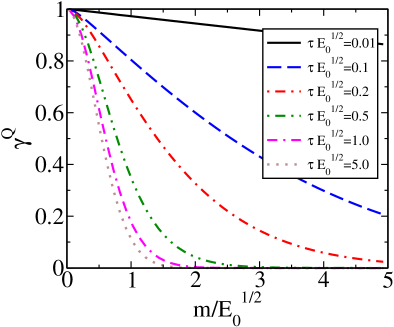
Figure 3: The suppression factor, $\gamma^{Q}$, at different pulse duration time as a function of the dimensionless mass parameter, $m/E_{0}^{1/2}$.

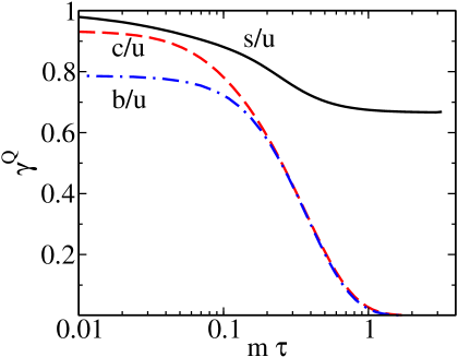
Figure 4: The suppression factor for heavy flavours at different values of $m\tau$.

In Fig. 1 the time evolution of quark number densities, $n_{q}$, are displayed for different pulse duration time, $\tau E_{0}^{1/2}=0.1$ and 0.5. For short pulse the quark number densities are comparable with each other (solid lines). In this case the particle production happens during the whole evolution of the field. In contrast to this, for long pulse, the number of produced charm and bottom quarks becomes negligible in the final state, because their production is balanced by annihilation. In U(1) color case the annihilation term can be identified clearly, see Ref. SkokLev05 .

This dependence on the pulse duration time is also demonstrated in Fig. 2. This figure clearly displays that both charm and bottom quark production is substantially enhanced in the cases of short pulse. This enhancement has a maximum at $\tau\sim 0.1\sqrt{E_{0}}$ for charm and at even smaller $\tau$ for heavier bottom quark. In opposite to the heavy quarks, light and strange quark productions are increasing with the pulse duration time without any local maximum.

Fig. 2 displays an important result that at small value of $\tau$ the heavy quark production has a pronounced maximum with value well beyond the well known asymptotic Schwinger estimate, see Ref. schw51 .

We further investigate the suppression factor and its dependence on pulse duration time and quark masses. Fig. 3 displays the suppression factor, $\gamma^{Q}$, for different pulse duration time, as a function of quark mass. For short pulse the suppression factor is decreasing almost linearly with increasing quark mass value. For long pulse we can see a very fast ($\sim\exp\{-m^{2}/E_{0}\}$) drop, which is consistent with the Schwinger formula.

In Fig. 4 we demonstrate the pulse duration time dependence of the suppression factor for different flavours. As it can be seen the dramatic change of the suppression factors for heavy quarks happens in the region $0.1<m\tau<1$. Actually, as it is shown in Appendix B, there are two dimensionless parameters that control the behaviour of the particle production. One is the dimensionless pulse duration, $m\tau$; the other is adiabaticity parameter, $\Gamma_{K}\sim m/({E_{0}\tau})$. The Schwinger formula is valid for the combination $m\tau\gg 1$ and $\Gamma_{K}\ll 1$.

Note, that at short pulse, the relative charm and bottom production is surprisingly large, which does not follow any earlier expectation.

IV.2 Energy and pulse duration time dependence

To fix free parameters we use the following simple model. The field depends on two unknown parameters, $\tau$ and $E_{0}$. We will fix them as the best fit of the suppression factors for primordial strange and charm quarks obtained in a quark coalescence calculation Levai:2000ne ; Levai:2008me at RHIC energy, $\sqrt{s}=200A$GeV. The suppression factors are $\gamma^{s}=0.88$ and $\gamma^{c}=6\cdot 10^{-2}$. The best fit reads $E_{0}=0.68$ GeV/fm and $\tau_{0}=0.134$ fm$/c$. Surprisingly, our simple model provides reasonable values for these parameters.

From intuitive reasons the duration of field pulse is proportional to the time of two Lorenz-contracted heavy ions pass each other at almost speed of light, i.e.

$$\tau\simeq\alpha\frac{2R}{\gamma_{cm}},$$ (40)

where $R$ is the radius of a nuclei, $\gamma_{cm}\simeq\sqrt{s}/(2{\rm GeV})$ is the gamma-factor, $\alpha$ is an unknown proportionality coefficient. In case of gold-gold collision at RHIC energy we obtained $\alpha=0.96$ from the best fit values given above. We further assume that $\alpha$ weakly depends on the collision energy and this dependence can be neglected. Thus having the value of $\alpha$ in hand we can transform the duration time dependence to the collision energy dependence. Although this conversion is oversimplified (e.g. it does not take into account any stopping effects), we expect to obtain results of the right order of magnitude. The extracted numbers make possible to interpret our numerical results on realistic basis, namely energy scales.

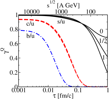
Figure 5: The suppression factor, $\gamma^{Q}$, for strange and heavy flavours as a function of pulse duration time and collision energy. The number marking the curves for strangeness suppression correspond to different values of $\beta$, see Eq. (41)

In Fig. 5 we show the time and energy dependence of the suppression factor for strange, charm and bottom quarks. To demonstrate how robust our results we calculated the suppression factors assuming different pulse duration time (corresponded to different collision energies) dependence of the field pulse magnitude $E_{0}(\tau)$. We consider three special cases

$$E_{0}(\tau)=E_{0}\cdot\left(\frac{\tau_{0}}{\tau}\right)^{\beta},\quad\beta=0,\ 1/2,\ 1.$$ (41)

The constant $E_{0}(\tau)$ is recovered if $\beta=0$. The second choice, $\beta=1/2$, corresponds to finite number of quarks for short pulses, $\tau\to 0$, (see Appendix B, Eq. (88)). Finally, $\beta=1$ results in divergent number of quarks for $\tau\to 0$ (see Appendix B, Eq. (91)).

In Fig. 5 we include these numbers, $\beta$, to distinguish between different cases for the strange quark suppression factor. For the heavy quarks all three curves are indistinguishable. As it can be seen, for strange quark the difference between the above cases is only important for low energy collisions, or long pulse duration. At constant $E_{0}$, and in the limit $\tau\to\infty$ the suppression factor for the strange quark production tends to the Schwinger limit, $\sim 0.74$. For charm and bottom quarks the Schwinger limit is negligibly small, see the suppression factor, $\gamma^{Q}$, for experimentally favoured energies in Table I.

	$\gamma_{\infty}$	130A GeV	200A GeV	1A TeV	2A TeV	5.5A TeV
s	0.74	0.84	0.88	0.96	0.98	0.99
c	3$\cdot 10^{-9}$	9$\cdot 10^{-3}$	0.06	0.66	0.82	0.91
b	$\sim 0$	$\sim$0	$10^{-6}$	0.15	0.45	0.72

Table 1: The suppression factor, $\gamma^{Q}$, for experimentally favoured energies. The calculations are done with a string tension $\kappa\simeq 1.17$, $\beta=0$. The result obtained by Schwinger formula is denoted by $\gamma_{\infty}$.

IV.3 Effective string tension

In the previous subsections we have obtained that the time dependence of the strong color field can induce an enhancement of heavy quark production (especially in a case of pulse duration times corresponded to high energy collisions). In usual string-based models FRITIOF ; HIJ ; RQMD ; QGSM ; HIJINGBB these abundances can be introduced by increasing the effective string tension in the Schwinger formula. However our results show that different effective string tensions should be introduced for different quark flavours. Here we calculate these string tension values and offer them for later use.

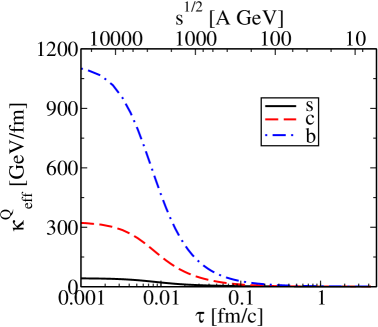
Figure 6: The effective string tension, $\kappa^{Q}_{eff}$, defined by Eq. (44) as a function of pulse duration time, $\tau$, and collision energy, $\sqrt{s}$.

Let us recall the Schwinger formula for particles with mass $m$

$$\frac{dN}{dtd^{3}x}=\frac{\kappa^{2}}{4\pi^{3}}\exp\left(-\frac{\pi m^{2}}{\kappa}\right).$$ (42)

Here $\kappa$ is the string tension. According to this formula the suppression factor of heavier ($Q$) to light quarks ($q$) is given by

$$\gamma^{Q}_{\infty}=\exp\left(-\frac{\pi(m_{Q}^{2}-m_{q}^{2})}{\kappa}\right).$$ (43)

This formula is valid for the case of arbitrary N in SU(N), see Ref. Gyulassy:1985 .

At first we extract an effective string tension assuming its common value for light and heavy quarks. Providing our numerical calculation of suppression factor (see Fig. 5) for Q-flavour, $\gamma^{Q}(\tau)$, we solve the equation

$$\gamma^{Q}_{\infty}(\kappa^{Q}_{{\rm eff}})=\gamma^{Q}(\tau)$$ (44)

to find the effective string tension dependence on pulse duration time, $\tau$, and subsequently on the collision energy, $\sqrt{s}$, for given quark flavour.

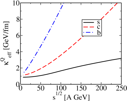
Figure 7: The same as in Fig. 6 in linear scales, but zoomed to RHIC energy range.

Fig. 6 displays results in a logarithmic scale. As it can be seen, the values of $\kappa^{Q}_{{\rm eff}}$ are very much different for strange, charm and bottom quarks. In Fig. 7 we show our results in a linear scale focusing on RHIC energy range. These large string tension values should be applied to light quark production as well, but we see three different values. This indicates the need of introduction of effective string tension in a different way.

We keep the usual string tension for light quark $\hat{\kappa}^{u}_{\rm eff}\simeq 1.17$ GeV/fm and introduce “flavour specific” effective string tensions for heavier flavours. On the basis of Eq.(42) we obtain the suppression factor

$$\hat{\gamma}^{Q}_{\infty}=\left(\frac{\hat{\kappa}^{Q}_{\rm eff}}{\hat{\kappa}^{u}_{\rm eff}}\right)^{2}\exp\left(-\pi\frac{m_{Q}^{2}}{\hat{\kappa}^{Q}_{\rm eff}}+\pi\frac{m_{u}^{2}}{\hat{\kappa}^{u}_{\rm eff}}\right).$$ (45)

Extracting such a “flavour specific” effective string tensions from the numerically calculated values we obtain Fig. 8 and Fig. 9. We would like to emphasize the difference between $\kappa^{Q}_{\rm eff}$ and $\hat{\kappa}^{Q}_{\rm eff}$, which is demonstrated by their different values.

Figure 8: The “flavour specific” effective string tension, $\hat{\kappa}^{Q}_{eff}$ as a function of pulse duration time, $\tau$, and collision energy, $\sqrt{s}$.

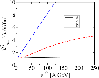
Figure 9: The same as in Fig. 8 in linear scales, but zoomed to RHIC energy range.

For easier use we generated the Table II displaying the “flavour specific” effective string tensions for experimentally favoured collision energies.

	130A GeV	200A GeV	1A TeV	2A TeV	5.5A TeV
u, d	1.17	1.17	1.17	1.17	1.17
s	1.24	1.26	1.32	1.33	1.34
c	3.32	4.2	6.1	6.3	6.5
b	10.3	14.7	32	36	38

Table 2: The “flavour specific” effective string tension, $\hat{\kappa}^{Q}_{\rm eff}$, values (in GeV/fm) for experimentally favoured energies.

The values for strange quark are approximately energy independent. However for charm and bottom quarks we get large values ($\sim 6-38$ GeV/fm). Earlier analysis Magas2002 indicated the evidences of large values for string tensions, $\kappa\sim 5-12$ GeV/fm. The applicability of such large values can be verified after performing proper string model based calculations. As it was demonstrated in Ref. Pop:2009sd , the available experimental data on charm production at RHIC (for $\sqrt{s}=200$A GeV) is successfully described by an effective string tension $\sim 3$ GeV/fm (the corresponding value in Table II is close to this result).

V Conclusion

We have calculated non-perturbative quark pair production in time-dependent strong non-Abelian SU(2) fields. Applying a pulse like time evolution and investigating the influence of pulse duration time, we observed that light and strange quark-pairs are produced as we expected, approaching the Schwinger limit. Charm and bottom quarks followed this behaviour for long pulses. However, for short pulses we did not see the expected heavy quark suppression, connected to the large quark mass in the Schwinger estimate. Indeed, the large value of inverse pulse duration time, overwhelming the mass of the heavy quark, $1/\tau\gg m_{c}$, determines the quark-pair production. We obtained enhanced heavy quark production at small duration time of the pulse, which can be connected to ultrarelativistic heavy ion collisions.

On the basis of our numerical results obtained from the kinetic equations we defined “flavour specific” effective string tension values to describe the enhanced heavy quark production. The validity of the obtained values must be verified by string based Monte-Carlo calculations. However our values seem to be reasonable in comparison to previously published string model results.

Finally, we would like to emphasis the strength of our model demonstrated in this paper: we are able to describe non-perturbative particle production (in strong non-Abelian field) in a wide energy range, simulating the environment of heavy ion collisions at different energies. The flexibility of our model is very much favoured to understand the experimental data and the physics behind them at different collisional energies. In the widely used CGC model Lappi:2006fp asymptotic solution could have been extracted displaying heavy ion reactions with infinite collisional energy, only. Our results, the obtained energy-dependent enhancement of non-perturbative heavy quark production, display the complexity of strong field physics and the importance of continuously varying energy dependence.

Appendix A. Kinetic equation for the Wigner function

The derivation of the kinetic equation for the Wigner function in non-Abelian case was discussed in details in Ref. HeinzOchs . The covariant proper time formulation of the kinetic equation was extended from earlier Abelian version Holl02 to non-Abelian one Prozor03 . In our investigation, here and earlier SkokLev07 ; Levai:2008wf , we use this non-Abelian version. However, the original paper of Prozorkevich et al. Prozor03 contains a few misprints in important equations, which may confuse the reader and questioning the validity of our work. To avoid this confusion we shortly display the most important steps for derivation of the kinetic equation for the Wigner function in non-Abelian case.

The starting point is the equations of motion for the quark field operators, obtained by the variation of the QCD Lagrangian. The last reads

$${\cal L}=\bar{\psi}(i\gamma^{\mu}D_{\mu}-m)\psi-\frac{1}{2}F_{\mu\nu}F^{\mu\nu},$$ (46)

where $D_{\mu}=\partial_{\mu}-igA_{\mu}$ is the covariant derivative, $A_{\mu}=A_{\mu}^{a}t^{a}$ is the 4-potential of color field, $m$ is the current quark mass and $g$ is the QCD coupling constant. The field tensor $F_{\mu\nu}$ is given by

$$F_{\mu\nu}=\frac{i}{g}\left[D_{\mu},D_{\nu}\right]=\partial_{\mu}A_{\nu}-\partial_{\nu}A_{\mu}-ig[A_{\mu},A_{\nu}].$$ (47)

The generators of SU(N) group in the fundamental representation $t_{a}=\lambda_{a}/2$ are expressed in terms of Gell-Mann matrices for SU(3) and Pauli matrices for SU(2).

The wanted equations of motion for spinor field operators read

$$\partial_{t}\psi = -\gamma^{0}\gamma^{i}D_{i}\psi-im\gamma_{0}\psi+igA_{0}\psi,$$ (48)

$$\partial_{t}\bar{\psi} = \bar{\psi}\gamma^{0}\gamma^{i}D_{i}^{*}+im\bar{\psi}\gamma_{0}-ig\bar{\psi}A_{0}.$$ (49)

Here the covariant derivative $D_{i}^{*}$ in the second equation acts to the left.

The single-time Wigner function HeinzOchs is defined by

$$W=$$ (50)

$$\int d^{3}ye^{i\mathbf{p}\mathbf{y}}U\left(\mathbf{x},\mathbf{x}+\frac{\mathbf{y}}{2}\right)\rho(\mathbf{x},\mathbf{y},t)U\left(\mathbf{x}-\frac{\mathbf{y}}{2},\mathbf{x}\right),$$

the unitary link operator $U(\mathbf{x}_{1},\mathbf{x}_{2})$ is introduced to maintain gauge invariance of the Wigner function. The link operator is given by

$$U({x}_{1},{x}_{2})=\exp\left\{ig\int_{x_{1}}^{x_{2}}dz^{\mu}A^{\mu}(z)\right\}.$$ (51)

The oneparticle density matrix reads

$$\rho^{ab}_{ik}=-\frac{1}{2}\left[\psi^{a}_{i}\left(\mathbf{x}+\frac{\mathbf{y}}{2}\right),\bar{\psi}^{b}_{k}\left(\mathbf{x}-\frac{\mathbf{y}}{2}\right)\right].$$ (52)

We apply the first derivative w.r.t. time to both sides of Eq. (50) and take into account that the variation of the link operator is given by

$$\delta U(x_{1},x_{2})=$$

$$ig\delta x_{1}^{\mu}A_{\mu}(x_{1})U(x_{1},x_{2})-ig\delta x_{2}^{\mu}U(x_{1},x_{2})A_{\mu}(x_{2})-$$

$$-ig\int_{0}^{1}dsU(x_{1},z)F_{\mu\nu}(z)U(z,x_{2})(x_{1}^{\mu}-x_{2}^{\mu})\times$$

$$\left\{\delta x_{2}^{\nu}+s(\delta x_{1}^{\nu}-\delta x_{2}^{\nu})\right\},\quad z=x_{2}+s(x_{1}-x_{2}).$$ (53)

Defining the Schwinger string

$$A^{[x_{1}]}(x_{2})=U(x_{1},x_{2})A(x_{2})U(x_{2},x_{1})$$ (54)

we rewrite Eq. (53)

$$\delta U(x_{1},x_{2})=\left\{ig\delta x_{1}^{\mu}A_{\mu}(x_{1})-ig\delta x_{2}^{\mu}A^{[x_{1}]}_{\mu}(x_{2})-\right.$$

$$-ig\int_{0}^{1}dsF^{[x_{1}]}_{\mu\nu}(z)(x_{1}^{\mu}-x_{2}^{\mu})\left.\left[\delta x_{2}^{\nu}+s(\delta x_{1}^{\nu}-\delta x_{2}^{\nu})\right]\right\}\times$$

$$U(x_{1},x_{2}).$$

Keeping in mind this variation we obtain the wanted equation for the Wigner function:

$$\partial_{t}W+\frac{1}{2}\left[\gamma^{0}\gamma^{i},\frac{\partial}{\partial x^{i}}W\right]+im[\gamma_{0},W]-ik_{i}\left\{\gamma_{0}\gamma^{i},W\right\}+$$

$$\frac{g}{2}\frac{\partial}{\partial k_{i}}\int_{0}^{1}ds\left\{E^{[x]}_{i}(\mathbf{z}^{-})W+WE^{[x]}_{i}(\mathbf{z}^{+})+\right.$$

$$\left.\frac{1}{2}F^{[x]}_{i\nu}(\mathbf{z}^{-})\left([W,\gamma^{0}\gamma^{\nu}]-s\left\{W,\gamma^{0}\gamma^{\nu}\right\}\right)\right.$$ (55)

$$\left.+\frac{1}{2}\left([W,\gamma^{0}\gamma^{\nu}]+s\left\{W,\gamma^{0}\gamma^{\nu}\right\}\right)F^{[x]}_{i\nu}(\mathbf{z}^{+})\right\}$$

$$-ig[A_{0},W]-\frac{1}{2}ig[\gamma_{0}\gamma^{i},[A_{i},W]]=0.$$

Here we used the equation of motions for fermion field operators and the following identity

$$\int f(\mathbf{y})\exp\left(i\mathbf{k}\mathbf{y}\right)d^{3}y=\int f\left(-i\frac{\partial}{\partial\mathbf{k}}\right)\exp\left(i\mathbf{k}\mathbf{y}\right)d^{3}y,$$ (56)

that is valid for any analytical function $f(\mathbf{y})$. The argument of field tensor is given by

$$\mathbf{z}^{\pm}=\mathbf{x}\pm i\frac{s}{2}\frac{\partial}{\partial\mathbf{k}}.$$ (57)

As we can see in Eq. (55), the obtained kinetic equation is nonlocal and difficult to solve numerically. With help of gradient expansion we can derive local approximations. In our calculations we use space homogeneous fields. In this case the kinetic equation take the form of Eq. (1), that we used in this paper and previous ones SkokLev07 ; Levai:2008wf .

The Wigner equation for the vacuum state follows from the definition displayed in Eq. (50). Indeed, using usual anticommutation relations for fermion field operators we obtain the Wigner function in vacuum

$$W^{ab}_{\rm v}=-\frac{m+\mathbf{k}\mathbf{\gamma}}{2\omega}\delta^{ab}.$$ (58)

Appendix B. Exact solutions for SU(2)-color case

In Section III the kinetic equation for the Wigner function was solved numerically. However, after taking into account additional symmetries of the external field we can discover further simplifications and even obtain exact solutions.

To demonstrate this fact we rewrite Eqs. (24-35) explicitly for the distribution function $f(\mathbf{k},t)$:

$$\partial_{t}f+\frac{3}{4}gE^{\diamond}_{z}\frac{\partial}{\partial k_{z}}f^{\diamond}=\frac{3}{4}W^{\diamond}v^{\diamond},$$ (59)

$$\partial_{t}v^{s}+\frac{3}{4}gE^{\diamond}_{z}\frac{\partial}{\partial k_{z}}v^{\diamond}=-\frac{3}{4}W^{\diamond}f^{\diamond}-2\omega u^{s},$$ (60)

$$\partial_{t}u^{s}+\frac{3}{4}gE^{\diamond}_{z}\frac{\partial}{\partial k_{z}}u^{\diamond}=2\omega v^{s},$$ (61)

$$\partial_{t}f^{\diamond}+gE^{\diamond}_{z}\frac{\partial}{\partial k_{z}}f=W^{\diamond}v^{s},$$ (62)

$$\partial_{t}v^{\diamond}+gE^{\diamond}_{z}\frac{\partial}{\partial k_{z}}v^{s}=\frac{1}{2}W^{\diamond}(1-2f)-2\omega u^{\diamond},$$ (63)

$$\partial_{t}u^{\diamond}+gE^{\diamond}_{z}\frac{\partial}{\partial k_{z}}u^{s}=2\omega v^{\diamond}.$$ (64)

Here the following new functions were defined

$$f^{\diamond} = \frac{ma^{\diamond}+\mathbf{k}\mathbf{b}^{\diamond}}{\omega},$$ (65)

$$v^{s,\diamond} = \frac{\varepsilon_{\perp}}{\omega}b_{z}^{s,\diamond}-\frac{k_{z}}{\omega}\left(\frac{ma^{s,\diamond}+k_{\perp}b^{s,\diamond}_{\perp}}{\varepsilon_{\perp}}\right),$$ (66)

$$u^{s,\diamond} = -\frac{k_{\perp}}{\varepsilon_{\perp}}d^{s,\diamond}-2\frac{m}{\varepsilon_{\perp}}c_{z}^{s,\diamond},$$ (67)

$$W^{\diamond} = \frac{gE\varepsilon_{\perp}}{\omega^{2}}.$$ (68)

The naming scheme is chosen to be consistent with the U(1) case of our previous work SkokLev05 . The transverse one-particle energy in Eq. (68) is defined by $\varepsilon_{\perp}=\sqrt{k_{\perp}^{2}+m^{2}}$.

As it follows from Eq. (23) the vacuum state corresponds to zero initial conditions for the functions $f,f^{\diamond}$, $v^{s,\diamond}$, $u^{s,\diamond}$.

Note, that Eqs. (59-64) has the same number of equation for massive and massless particles. Thus the massless limit does not lead to any further simplifications. The system (59-64) can be transformed to more conventional form, allowing the solution on characteristics. For that we introduce the following new functions

$$F^{\pm} = f\pm\frac{\sqrt{3}}{2}f^{\diamond},$$ (69)

$$V^{\pm} = v^{s}\pm\frac{\sqrt{3}}{2}v^{\diamond},$$ (70)

$$U^{\pm} = u^{s}\pm\frac{\sqrt{3}}{2}u^{\diamond}.$$ (71)

The equations for these functions read

$$\partial_{t}F^{\pm}\pm\frac{\sqrt{3}}{2}gE^{\diamond}_{z}\frac{\partial}{\partial k_{z}}F^{\pm} = \pm\frac{\sqrt{3}}{2}W^{\diamond}V^{\pm},$$ (72)

$$\partial_{t}V^{\pm}\pm\frac{\sqrt{3}}{2}gE^{\diamond}_{z}\frac{\partial}{\partial k_{z}}V^{\pm} = \pm\frac{\sqrt{3}W^{\diamond}}{4}(1-2F^{\pm})-$$ (73)

$$-2\omega U^{\pm},$$

$$\partial_{t}U^{\pm}\pm\frac{\sqrt{3}}{2}gE^{\diamond}_{z}\frac{\partial}{\partial k_{z}}U^{\pm} = 2\omega V^{\pm}.$$ (74)

The equations for “(+)” and “(–)” functions are completely factorized and can be solved independently. The distribution function $f$ is obtained as

$$f=\frac{F^{+}+F^{-}}{2}.$$ (75)

The equations (72-74) are very similar to those obtained in the Abelian case (see Eqs. (76-77) in Pervushin:2006vh and Eqs. (22-24) in SkokLev05 ). However, only $f$ is physical quantity, while the functions $F^{\pm}$ carry intermediate information. Nevertheless, from mathematical point of view there is no difference and this analogy allows to exploit U(1) solution to obtain exact analytical results for SU(2)-color case, as we demonstrate below.

In the case of a time reversal symmetry of the field strength, $E(t)=E(-t)$, the corresponding components are equal to each other, e.g. $F^{+}=F^{-}$. Thus the distribution function is defined as $f=F^{+}=F^{-}$. Furthermore in the Abelian case it is known that for the field with form of Eq. (37) an analytic solution of Dirac equation exists, as well as analytic solution of the corresponding kinetic equation (see e.g. Ref. grib94 ). Following this analogy we can obtain an analytic solution of Eqs. (72-74) in the asymptotic state $t\gg\tau$:

$$f=\frac{\sinh\left(\pi(\theta-\mu^{+}+\mu^{-})\right)\sinh\left(\pi(\theta+\mu^{+}-\mu^{-})\right)}{\sinh(2\pi\mu^{+})\sinh(2\pi\mu^{-})}.\quad\quad$$ (76)

Here we introduced the following notations

$$\mu^{\pm}=\frac{\tau}{2}\sqrt{\left(k_{z}\pm\frac{E_{0}}{E_{cr}}m^{2}\tau\right)^{2}+k_{\perp}^{2}+m^{2}},$$ (77)

$$\theta=-\frac{E_{0}}{E_{cr}}m^{2}\tau^{2},$$ (78)

$$E_{cr}=\frac{2m^{2}}{\sqrt{3}g}.$$ (79)

The Schwinger limit can be readily obtained from Eq. (76). Indeed, for pulses longer than any scale in the system, $\tau\gg{\rm max}\{E_{0}^{-1/2},m^{-1/2}\}$, we can use the expansions

$$\theta\pm(\mu^{+}-\mu^{-})=-\frac{E_{0}}{E_{cr}}m^{2}\tau^{2}\mp k_{3}\tau+{\cal O}\left(\frac{1}{\tau}\right),$$ (80)

$$\mu^{\pm}=\frac{E_{0}}{2E_{cr}}m^{2}\tau^{2}\pm k_{3}\tau+\frac{2}{\sqrt{3}}\frac{m^{2}+k_{\perp}^{2}}{4gE_{0}}+{\cal O}\left(\frac{1}{\tau}\right).\ \ \quad$$ (81)

In the leading order of expansion parameter $\tau$ we obtain the following distribution function

$$f\simeq\exp\left(-\pi\frac{2\varepsilon_{\perp}}{\sqrt{3}gE_{0}}\right).$$ (82)

After the integration w.r.t. momentum we obtain SU(2) version of the Schwinger formula

$$n=\tau\frac{3(gE_{0})^{2}}{16\pi^{2}}\exp\left(-\frac{2\pi m^{2}}{\sqrt{3}gE_{0}}\right),$$ (83)

where we have taken into account the replacement $\int dk_{z}\to\sqrt{3}gE_{0}\tau/2$. Thus in SU(2) the suppression factor of heavy particles with mass $m_{Q}$ to light particles with mass $m_{q}$ in Schwinger limit is given by

$$\gamma^{Q}=\exp\left(-\frac{2\pi(m_{Q}^{2}-m_{q}^{2})}{\sqrt{3}gE_{0}}\right).$$ (84)

The analytical result for the number density of quarks can be also obtained if the following inequality is satisfied

$$\Gamma_{K}\equiv\frac{E_{cr}}{E}\frac{1}{m\tau}\gg{\rm max}\{1,m\tau\},$$ (85)

where we introduce the adiabaticity parameter $\Gamma_{K}$ . In this limit the dictribution function is given by

$$f\simeq\left(\frac{\sqrt{3}\pi\sqrt{k_{\perp}^{2}+m^{2}}}{2\omega}gE\tau^{2}{\rm csch}\left(\pi\omega\tau\right)\right)^{2}.$$ (86)

The momentum integration of this distribution function can be done analytically in the following cases:

• Long pulse duration and undercritical field. For long pulse duration the constraint $m\tau\gg 1$ in Eq. (85) is satisfied for undercritical field, $E/E_{cr}\ll 1$. After expanding the distribution function in Eq. (86) and performing momentum integration, we obtain the number density

  $$n=\frac{3(m\tau)^{3/2}}{4\pi}\tau(gE_{0})^{2}\exp(-2\pi m\tau).$$ (87)

  The condition of long pulse duration and undercritical field could be realized for the collision of heavy ions in SPS energy range (assuming that the physical picture of classical gluon field is still valid) for light quarks, or for charm and bottom quarks at and below the RHIC energies (the string tension is the order of $1$ GeV/fm.)

• Short pulse duration. In the opposite limit, $m\tau\ll 1$, we obtain the number density

  $$n\simeq\frac{\tau}{12\pi}(gE_{0})^{2}.$$ (88)

  In this case the number density of produced particles depends linearly on the duration time, $\tau$, and is independent of the particle mass, $m$.

  For the parameter set we used in the main part of the manuscript the field magnitude, $E_{0}$, is about five times higher than the critical one for the strange quark. The number of produced strange quarks follows the Eq. (88) for pulse duration at least five times less then inverse mass of strange quark $\tau\ll(5m_{s})^{-1}\simeq 0.3$ fm$/c$ As we estimated in Eq. (40) the pulse duration time for RHIC is about $0.1$ fm/c, that is only three times less than $(5m_{s})^{-1}$. Thus the expression (88) is valid for the strange quark only at higher than RHIC energies.

  For heavier particles, e.g. charm quark, the requirement $m_{c}\tau\ll 1$ leads to smaller values of $\tau$. Indeed, we can rewrite

  $$m_{c}\tau=\frac{m_{c}}{m_{s}}\times(m_{s}\tau)\ll 1.$$ (89)

  This expression shows that Eq. (88) becomes valid for charm quark on a shorter scale of pulse duration time ($m_{c}/m_{s}\simeq 8$).

  For light quarks the condition $m_{u}\tau\ll 1$ is trivially satisfied at RHIC energies. However now the condition (85) plays more important role. From Eq. (85) we obtain an estimate for the validity of Eq. (88)

  $$\tau\ll 4\cdot 10^{-3}{\rm fm}/c.$$ (90)

  In this limiting case the strange suppression factor tends to unity, that supports our numerical result in Fig. 5..

One more analytical result can be obtained from the general solution Eq. (76). If the duration time of the pulse tends to zero, but amplitude is increasing as $E_{0}=A_{0}\tau^{-1}$ ($A_{0}$ is constant), then the distribution function is given by

$$f=\frac{1}{2}\left(1-\frac{\omega^{2}-\frac{3}{4}A_{0}^{2}}{\omega_{+}\omega_{-}}\right).$$ (91)

where $\omega_{\pm}=2\mu_{\pm}/\tau$. Since the momentum integral from the above distribution function is divergent, this approximation results in infinitely many new quark-antiquark pairs in unit volume. This is understandable since we pump infinite energy to the system in this special case.

References

- (1) J. Schwinger, Phys. Rev. 82 (1951) 664.
- (2) J. Adams et al. [STAR Collaboration], Phys. Rev. Lett. 94, 062301 (2005) [arXiv:nucl-ex/0407006].
- (3) S. L. Baumgart [STAR Collaboration], arXiv:0805.4228 [nucl-ex].
- (4) B. I. Abelev et al. [STAR Collaboration], arXiv:0805.0364 [nucl-ex].
- (5) A. Adare et al. [PHENIX Collaboration], Phys. Rev. Lett. 97, 252002 (2006) [arXiv:hep-ex/0609010].
- (6) A. Adare et al. [PHENIX Collaboration], Phys. Rev. Lett. 98, 172301 (2007) [arXiv:nucl-ex/0611018].
- (7) Quark Matter’08 Conference Proceedings (Ed. by Feng Liu, Zhigang Xiao, Pengfei Zhuang), J. Phys. G 36 (2009).
- (8) A. D. Frawley, T. Ullrich, and R. Vogt, Phys. Rept. 462, 125 (2008) [arXiv:0806.1013 [nucl-ex]].
- (9) V. Topor Pop, J. Barrette, and M. Gyulassy, Phys. Rev. Lett. 102, 232302 (2009) [arXiv:0902.4028 [hep-ph]].
- (10) B. Andersson et al., Phys. Rep. 97 (1983) 31; Nucl. Phys. B281 (1987) 289.
- (11) X.N. Wang and M. Gyulassy, Phys. Rev. D44 (1991) 3501; Comput. Phys. Commun. 83 (1994) 307.
- (12) H. Sorge, Phys. Rev. C52 (1995) 3291.
- (13) N. S. Amelin, K. K. Gudima, S. Y. Sivoklokov, and V. D. Toneev, Sov. J. Nucl. Phys. 52, 172 (1990) [Yad. Fiz. 52, 272 (1990)].
- (14) V. Topor Pop, M. Gyulassy, J. Barrette, C. Gale, X. N. Wang, and N. Xu, Phys. Rev. C 70, 064906 (2004) [arXiv:nucl-th/0407095].
- (15) M. Gyulassy and L. McLerran, Phys. Rev. C56 (1997) 2219.
-
(16)
V. Topor Pop, M. Gyulassy, J. Barrette, C. Gale, R. Bellwied, and N. Xu,
Phys. Rev. C 72, 054901 (2005);
V. Topor Pop, M. Gyulassy, J. Barrette, C. Gale, S. Jeon, and R. Bellwied, arXiv:hep-ph/0608136;
Phys. Rev. C 75, 014904 (2007). - (17) T. Lappi and L. McLerran, Nucl. Phys. A 772, 200 (2006) [arXiv:hep-ph/0602189].
- (18) L. D. McLerran, Lect. Notes Phys. 583, 291 (2002) [arXiv:hep-ph/0104285].
- (19) V. K. Magas, L. P. Csernai, and D. Strottman, Nucl. Phys. A 712, 167 (2002) [arXiv:hep-ph/0202085].
- (20) E. Iancu and R. Venugopalan, hep-ph/0303204 and references therein.
- (21) F. Gelis and R. Venugopalan, Nucl. Phys. A 776, 135 (2006) [arXiv:hep-ph/0601209].
- (22) F. Gelis and R. Venugopalan, Nucl. Phys. A 779, 177 (2006) [arXiv:hep-ph/0605246].
- (23) J. P. Blaizot, F. Gelis, and R. Venugopalan, Nucl. Phys. A 743, 57 (2004) [arXiv:hep-ph/0402257].
- (24) G. Gatoff, et al. Phys. Rev. D36 (1987) 114.
- (25) Y. Kluger et al., Phys. Rev. Lett. 67 (1991) 2427.
- (26) G. Gatoff and C.Y. Wong, Phys. Rev. D46 (1992) 997.
- (27) C.Y. Wong, et al. Phys. Rev. D51 (1995) 3940.
- (28) J.M. Eisenberg, Phys. Rev. D51 (1995) 1938.
- (29) D.V. Vinnik, et al., Few-Body Syst. 32 (2002) 23 .
- (30) V.N. Pervushin, et al. accepted in Int. Mod. Phys. A. (hep-th/0307200).
- (31) A. V. Prozorkevich, et al. Phys. Lett. B 583 (2004) 103 [arXiv:nucl-th/0401056].
- (32) V. N. Pervushin and V. V. Skokov, Acta Phys. Polon. B 37, 2587 (2006) [arXiv:astro-ph/0611780].
- (33) B. Mihaila, F. Cooper, and J. F. Dawson, arXiv:0905.1360 [hep-ph].
- (34) J. F. Dawson, B. Mihaila, and F. Cooper, arXiv:0906.2225 [hep-ph].
- (35) A.V. Prozorkevich, S.A. Smolyansky, and S.V. Ilyin, (hep-ph/0301169).
- (36) H. T. Elze, M. Gyulassy, and D. Vasak, Phys. Lett. B 177, 402 (1986); H. T. Elze, M. Gyulassy, and D. Vasak, Nucl. Phys. B 276, 706 (1986); S. Ochs and U. Heinz, Ann. Phys. 266 (1998) 351.
- (37) D.D. Dietrich, Phys. Rev. D68 (2003) 105005; ibid. D70 (2004) 105009.
- (38) V.V. Skokov and P. Levai, Phys. Rev. D71 (2005), 094010, (hep-ph/0410339).
- (39) V. V. Skokov and P. Levai, Phys. Rev. D78 (2008) 054004, (arXiv:0710.0229 [hep-ph]).
- (40) P. Levai and V. Skokov, J. Phys. G: Nucl. Part. Phys. 36 (2009) 064068 [arXiv:0812.2536].
- (41) P. Levai, T. S. Biro, P. Csizmadia, T. Csorgo and J. Zimanyi, J. Phys. G 27, 703 (2001) [arXiv:nucl-th/0011023].
- (42) P. Levai, J. Phys. G 35, 044041 (2008) [arXiv:0806.0133 [nucl-th]].
- (43) M. Gyulassy and A. Iwazaki, Phys. Lett. 165B, 157 (1985).
- (44) A. Höll, V.G. Morozov, and G. Röpke, Ther. Math. Phys. 131, 812 (2002); Ther. Math. Phys. 132, 1029 (2002).
- (45) A.A. Grib, S.G. Mamaev, and V.M. Mostepanenko, Vacuum Quantum Effects in Strong Fields, (Friedmann Laboratory Publishing, St. Petersburg, 1994); G. V. Dunne, arXiv:hep-th/0406216; K. Fukushima, F. Gelis and T. Lappi, arXiv:0907.4793 [hep-ph].