Relativistic RPA in axial symmetry

Abstract

Covariant density functional theory, in the framework of self-consistent Relativistic Mean Field (RMF) and Relativistic Random Phase approximation (RPA), is for the first time applied to axially deformed nuclei. The fully self-consistent RMF+RRPA equations are posed for the case of axial symmetry and non-linear energy functionals, and solved with the help of a new parallel code. Formal properties of RPA theory are studied and special care is taken in order to validate the proper decoupling of spurious modes and their influence on the physical response. Sample applications to the magnetic and electric dipole transitions in ²⁰Ne are presented and analyzed.

I Introduction

New experimental facilities with radioactive nuclear beams have stimulated enhanced experimental and theoretical efforts to understand the structure of nuclei, not only along the narrow line of stable isotopes, but also in areas of large neutron- and proton excess far from the valley of $\beta$-stability. Beside the investigation of the ground state properties of these nuclei, more and more experimental studies are being devoted to the understanding of the properties of excited states in this region.

On the theoretical side, only very light nuclei can be studied in the framework of modern ab initio methods. Shell model calculations in restricted configuration spaces provide an accurate description of light and medium-heavy nuclei. For the large majority of nuclei, however, a quantitative microscopic description is only possible using density functional theory (DFT). Although DFT can, in principle, provide an exact description of the many-body dynamics if the exact density functional is known HK.64 ; KS.65 , in nuclear physics one is far from a microscopic derivation of this functional and in addition there is the problem, that in self-bound systems density functional theory can only be applied to intrinsic densites Eng.07 ; Gir.08 . The most successful schemes use a phenomenological ansatz incorporating as many symmetries as possible, and adjust the parameters of these functionals to ground state properties of characteristic nuclei all over the periodic table (for a recent review see Ref. BHR.03 ).

Of particular interest are covariant density functionals Rin.96 ; VALR.05 because they are based on Lorentz invariance. The inclusion of this symmetry not only allows for the description of the spin-orbit part of the nuclear interaction in a natural and consistent way, but it also puts considerable restrictions on the number of parameters in the corresponding functionals, all without reducing the quality of the agreement with experimental data. A very successful example is the Relativistic Hartree-Bogoliubov model GEL.96 ; VALR.05 , which combines a density dependence through a non-linear coupling between the meson fields BB.77 with pairing correlations based on an effective interaction of finite range GEL.96 .

Excited states are described within this formalism by time-dependent density functional theory VBR.95 . In the small amplitude limit one obtains the relativistic Random Phase Approximation (RRPA) RS.80 ; RMG.01 . This method provides a natural framework to investigate collective and non-collective excitations of $ph$-character. Although several RRPA implementations have been available since the eighties Fur.85 , only very recently RRPA-based calculations have reached a level on which a quantitative comparison with experimental data became possible MWG.02 . And even though the self-consistent relativistic mean-field (RMF) framework has been employed in many studies of deformed nuclei PRB.87 ; GRT.90 , applications of the relativistic RRPA method have so far restricted to spherical nuclei. This is also true for non-relativistic density functionals, where most of the RPA-calculations are restricted to spherical nuclei. Only very few deformed RPA calculations based on Skyrme HHR.98 ; NKK.06 or Gogny forces PGB.07 are available so far.

On the other hand, it is well known that only semi-magic nuclei have spherical shape, and that most of the other nuclei in the nuclear chart are deformed. Thus, the description of the collective response of these nuclei can only be accomplished within a framework where deformation is explicitly taken into account. From the point of view of nuclear structure the motivation for deformed RPA calculations is evident. In addition, the nuclear electric dipole response obtained in this framework provides valuable input for the calculation of important astrophysical processes Gor.98 , such as the $r$- or the $s$-process, that pass though large areas of deformed nuclei.

In this manuscript we report on the extension of relativistic RPA theory to axially deformed nuclei and its application to the study of collective excitations. In section II we discuss the underlying density functional and the derivation of the relativistic RPA equations. Section III deals with specific aspects of RMF and RPA theory in deformed systems and the evaluation of the relativistic RPA matrix elements in the basis of axially deformed Dirac spinors. Section IV is devoted to strength functions and sum rules and in section V we discuss transition densities in the intrinsic and in the laboratory frame. Violations of symmetries and the corresponding Goldstone modes are treated in Section VI and in section VII we show illustrative applications in ²⁰Ne, in particular its magnetic and electric dipole response. Finally section VIII contains the summary and an outlook.

II The covariant energy density functional and the relativistic RPA equations

At the moment the most successful density functionals in nuclear physics are purely phenomenological. Considering from the beginning as many symmetries as possible, one starts with a relatively simple ansatz for the energy density functional VB.72 ; DG.80 ; Wal.74 , which contains a certain number of phenomenological parameters. One then adjusts these parameters to bulk properties of nuclear matter and to ground state properties of a few selected finite nuclei with spherical shape. These sets are then used over the entire nuclear chart. It turns out that for a good description of the experiment data, it is crucial to allow for a density dependence in this ansatz. the concept of density dependence has its origin in more microscopic theories of the nuclear many-body system, such as Brueckner theory Bru.54 , which leads to a density dependent effective interaction in the nuclear interior. In relativistic models this density dependence was taken into account in the form of a non-linear meson coupling in Ref. BB.77 or in the form of density dependent meson-nucleon couplings in Ref. BT.92 . If the ansatz is chosen properly and if the adjustment of the phenomenological parameters is carefully done, the quantitative agreement with available experimental data is remarkable BHR.03 ; VALR.05 .

In this work we concentrate on relativistic density functional theory Rin.96 ; VALR.05 . These functionals are based on Lorentz invariance. The basic degrees of freedom are the nucleons described by point-like Dirac spinors. In order to be consistent with Lorentz invariance and causality, one has two possibilities for introducing an interaction between these particles. Either one restricts the theory to zero range interactions, as it is done in Nambu Jona-Lasinio models  NJL.61a , or one allows for the exchange of effective mesons. Since it is well know since the early days of Skyrme theory that pure $\delta$-forces are not sufficient to describe at the same time nuclear binding energies and radii, and since gradient terms in the Lagrangian can lead to certain difficulties in the relativistic formulation, historically the second method was the first to be used Wal.74 ; BB.77 . Only recently relativistic point coupling models with density dependent coupling constants have been employed successfully in nuclear physics BMM.02 .

For simplicity we concentrate in this work on meson exchange models with non-linear meson couplings. Of course, the corresponding equations can be easily extended to meson coupling models with density dependent vertices TW.99 ; DD-ME1 ; DD-ME2 or to relativistic point coupling models BMM.02 .

In covariant density functionals with meson exchange, the nucleons are described by Dirac spinors coupled by the exchange of mesons and by the electromagnetic field through an effective Lagrangian. The starting point for a phenomenological ansatz is therefore the Walecka model Wal.74 . The mesons are classified by there quantum numbers, spin, parity and isospin ($I^{\pi},T$). In the isoscalar channel one has the scalar $\sigma$-meson ($I^{\pi}=0^{+},T=0$), and the vector $\omega$-meson ($I^{\pi}=1^{-},T=0$), and in the isovector channel one considers only the vector $\rho$-meson ($I^{\pi}=1^{-},T=1$). The $\delta$-meson ($I^{\pi}=0^{+},T=1$) is not included because, so far, there is not enough data in low energy nuclear structure physics to fix its parameters uniquely. In addition, the pion is not taken into account because, again for the sake of simplicity, we work only at the Hartree level, which forbids the appearance of the parity violating pion-field. The essential contributions of pionic degrees of freedom by two-pion exchange are taken care of in a phenomenological way by the $\sigma$-meson. Therefore, the starting point is an effective Lagrangian density of the form

$$\mathcal{L}=\mathcal{L}_{N}+\mathcal{L}_{m}+\mathcal{L}_{int}.$$ (1)

$\mathcal{L}_{N}$ refers to the Lagrangian of the free nucleon

$$\mathcal{L}_{N}=\bar{\psi}(i\gamma^{\mu}\partial_{\mu}-m)\psi,$$ (2)

where $m$ is the bare nucleon mass and $\psi$ denotes the Dirac spinor. $\mathcal{L}_{m}$ is the Lagrangian of the free meson fields and the electromagnetic field

$$\mathcal{L}_{m} =\frac{1}{2}\partial_{\mu}\sigma\partial^{\mu}\sigma-\frac{1}{2}m_{\sigma}^{2}\sigma^{2}-\frac{1}{4}\Omega_{\mu\nu}\Omega^{\mu\nu}+\frac{1}{2}m_{\omega}^{2}\omega_{\mu}\omega^{\mu}$$

$$-\frac{1}{4}\vec{R}_{\mu\nu}\vec{R}^{\mu\nu}+\frac{1}{2}m_{\rho}^{2}\vec{\rho}_{\mu}\vec{\rho}^{\mu}-\frac{1}{4}F_{\mu\nu}F^{\mu\nu}$$ (3)

with the corresponding masses $m_{\sigma}$, $m_{\omega}$, $m_{\rho}$, and the field tensors

$$\Omega_{\mu\nu} =\partial_{\mu}\omega_{\nu}-\partial_{\nu}\omega_{\mu},$$

$$\vec{R}_{\mu\nu} =\partial_{\mu}\vec{\rho}_{\nu}-\partial_{\nu}\vec{\rho}_{\mu},$$ (4)

$$F_{\mu\nu} =\partial_{\mu}A_{\nu}-\partial_{\nu}A_{\mu},$$

where arrows denote isovectors and boldface symbols vectors in 3-dimensional $r$-space. The interaction Lagrangian $\mathcal{L}_{int}$ is given by minimal coupling terms

$$\mathcal{L}_{int}=-g_{\sigma}\bar{\psi}\Gamma_{\sigma}\sigma\psi-g_{\omega}\bar{\psi}\Gamma_{\omega}^{\mu}\omega_{\mu}\psi-g_{\rho}\bar{\psi}\vec{\Gamma}_{\rho}^{\mu}\vec{\rho}_{\mu}\psi-e\bar{\psi}\Gamma_{e}^{\mu}A_{\mu}\psi$$ (5)

with the vertices

$$\Gamma_{\sigma}=1,\quad\Gamma_{\omega}^{\mu}=\gamma^{\mu},\quad\vec{\Gamma}_{\rho}^{\mu}=\gamma^{\mu}\vec{\tau},\quad\Gamma_{e}^{\mu}=\dfrac{1}{2}(1-\tau_{3})\gamma^{\mu},$$ (6)

where $g_{\sigma}$, $g_{\omega}$, $g_{\rho}$ and $e$ are the respective coupling constants for the $\sigma$, $\omega$, $\vec{\rho}$ and photon fields. This yields to

$$\mathcal{L}_{int}=-\sum_{m}g_{m}\bar{\psi}\Gamma_{m}\phi_{m}\psi,$$ (7)

where the index $m$ runs over the various meson and electromagnetic fields, and also over the Lorentz index for vector mesons and isospin indices for mesons carrying isospin

$$\phi_{m}=(\sigma,\omega^{\mu},\vec{\rho}^{\mu},A^{\mu}),\qquad\Gamma_{m}=(\Gamma_{\sigma},\Gamma_{\omega}^{\mu},\vec{\Gamma}_{\rho}^{\mu},\Gamma_{e}^{\mu}).$$ (8)

Already in the earliest applications of the RMF framework it was realized, however, that this simple linear interaction density functional did not provide a quantitative description of complex nuclear systems; an effective density dependence needs to be introduced. Historically, the first BB.77 was the inclusion of non-linear self-interaction terms in the meson part of the Lagrangian in the form of a quartic $\sigma$ potential

$$\frac{1}{2}m_{\sigma}^{2}\sigma^{2}+U(\sigma)$$ (9)

with

$$U(\sigma)=\frac{g_{2}}{3}\sigma^{3}+\frac{g_{3}}{4}\sigma^{4},$$ (10)

which includes the non-linear $\sigma$ self-interactions with two additional parameters $g_{2}$ and $g_{3}$. This particular form of the non-linear potential has become standard in applications of RMF functionals, although additional non-linear interaction terms, both in the isoscalar and isovector channels, have been considered over the years Bod.91 ; TM1 ; SFM.00 ; HP.01 .

Two other approaches, of more recent development, can also be found in the literature, based on the introduction of the density dependence directly in the coupling constants TW.99 ; DD-ME1 ; DD-ME2 and on the expansion of the meson propagators into zero-range couplings and gradient corrections terms BMM.02 . For the sake of simplicity we will restrict the discussion in this work to non-linear density functionals, always taking the NL3 NL3 parameter set as the force of choice. Also, the explicit inclusion of the non-linear meson potential $U(\sigma)$ is generally avoided in order to keep the formulation as clean as possible. But, of course, it is included in all numerical calculations of results presented in the manuscript, and it shall be explicitly mentioned at certain important points in the following discussions.

The Hamiltonian density can be derived from the Lagrangian density of Eq. (1) as the (0,0) component of the energy-momentum tensor

$$\mathcal{H}=T^{00}=\frac{\partial\mathcal{L}}{\partial\dot{q}_{j}}\dot{q}_{j}-\mathcal{L},$$ (11)

leading the to the energy functional

$$E[\hat{\rho},\phi]=\int\mathcal{H}d^{3}r.$$ (12)

Following the Kohn-Sham approach KS.65 ; KS.65a , one can express the relativistic energy density $E$ as a functional of the relativistic single particle density matrix

$$\hat{\rho}(\boldsymbol{r},\boldsymbol{r}^{\prime},t)={\displaystyle\sum\limits_{i}^{A}}\psi_{i}(\boldsymbol{r}\mathbf{,}t)\psi_{i}^{\dagger}(\boldsymbol{r}^{\prime},t)$$ (13)

and the meson fields $\phi=(\sigma$,$\omega$,$\rho$,$\gamma)$. The sum over $i$ in Eq. (13) runs over the orbits in the Dirac sea (no-sea approximation, see below). Considering the 4-dimensional Dirac spinor $\psi_{i}$ as a column vector and $\psi_{i}^{\dagger}$ as a row vector one concludes that $\hat{\rho}(\boldsymbol{r},\boldsymbol{r}^{\prime},t)$ is a 4x4 matrix in Dirac space. This leads to the standard relativistic energy density functional

$$E_{RMF}[\hat{\rho},\phi] =\mathrm{Tr}[(-i\boldsymbol{\alpha}\boldsymbol{\nabla}+\beta m)\hat{\rho}]+\mathrm{Tr}[(\beta\Gamma_{m}\phi_{m})\hat{\rho}]$$

$$\pm\frac{1}{2}\int d^{3}r\left[(\partial_{\mu}\phi_{m})^{2}+m_{m}^{2}\right],$$ (14)

where summation over the different mesons is implied, and the trace operation involves summation over Dirac indices and an integral over the whole space. $\Gamma_{m}$ describes the structure of the meson-nucleon interaction. The upper sign in Eq. (14) holds for the scalar mesons and the lower sign for the vector mesons. At the mean field level the mesons are treated as classical fields. The nucleons, described by a Slater determinant $|\Phi\rangle$ of single-particle wave functions, move independently in these classical meson fields. One can thus apply the classical time-dependent variational principle

$$\delta\int_{t_{1}}^{t_{2}}dt\{\langle\Phi|i\partial_{t}|\Phi\rangle-E[\hat{\rho},\phi]\}=0,$$ (15)

which leads to the equations of motion

$$i\partial_{t}\hat{\rho} =\left[h[\hat{\rho},\phi],\hat{\rho}\right],$$ (16)

$$\left[\partial^{\nu}\partial_{\nu}+m_{m}^{2}\right]\phi_{m} =\mp\mathrm{Tr}\left[\beta\Gamma_{m}\hat{\rho}\right],$$ (17)

where the single particle effective Dirac Hamiltonian $\hat{h}$ is the functional derivative of the energy with respect to the single particle density

$$\hat{h}[\hat{\rho},\phi]=\frac{\delta E[\hat{\rho},\phi]}{\delta\hat{\rho}}=(-i\boldsymbol{\alpha}\boldsymbol{\nabla}+\beta m)+{\displaystyle\sum\limits_{m}}\beta\Gamma_{m}\phi_{m}.$$ (18)

The time-dependent Dirac equation for the nucleons reads

$$\left[\gamma^{\mu}\left(i\partial_{\mu}+V_{\mu}\right)+m+S\right]\psi_{k}=0$$ (19)

with the scalar $S$ and vector $V_{\mu}$ potentials

$$S(\boldsymbol{r},t) =g_{\sigma}\sigma(\boldsymbol{r},t),$$ (20)

$$V_{\mu}(\boldsymbol{r},t) =g_{\omega}\omega_{\mu}(\boldsymbol{r},t)+g_{\rho}\vec{\tau}\vec{\rho}_{\mu}(\boldsymbol{r},t)+eA_{\mu}(\boldsymbol{r},t)\frac{1-\tau_{3}}{2}.$$

and the time-dependent meson equations have the form

$$\left[\partial^{\nu}\partial_{\nu}+m_{\sigma}^{2}\right]\sigma =-g_{\sigma}\rho_{s}$$ (21)

$$\left[\partial^{\nu}\partial_{\nu}+m_{\omega}^{2}\right]\omega^{\mu} =+g_{\omega}j^{\mu}$$ (22)

$$\left[\partial^{\nu}\partial_{\nu}+m_{\rho}^{2}\right]\vec{\rho}^{\mu} =+g_{\rho}\vec{j}_{\text{tv}}^{\mu}$$ (23)

$$\left[\partial^{\nu}\partial_{\nu}\right]A^{\mu} =+ej_{\text{c}}^{\mu}$$ (24)

with the sources

$$\mathrm{scalar-isoscalar}\qquad\rho_{s}=\sum_{i}^{A}\bar{\psi}_{i}\psi_{i},$$ (25)

$$\mathrm{vector-isoscalar}\qquad j^{\mu}=\sum_{i}^{A}\bar{\psi}_{i}\gamma^{\mu}\psi_{i},$$ (26)

$$\mathrm{vector-isovector}\qquad\vec{j}_{\text{tv}}^{\mu}=\sum_{i}^{A}\bar{\psi}_{i}\gamma^{\mu}\vec{\tau}\psi_{i},$$ (27)

$$\mathrm{electromagnetic}\qquad j_{\text{c}}^{\mu}=\sum_{i}^{A}\bar{\psi}_{i}\gamma^{\mu}\frac{1}{2}(1-\tau_{3})\psi_{i}$$ (28)

In order to describe the ground state properties of even-even nuclei, one has to look for stationary time-reversal invariant solutions of the equations of motion Eq. (16) and Eq. (17). The nucleon wave functions are then the eigenvectors of the stationary Dirac equation,

$$\left[-i\boldsymbol{\alpha}\boldsymbol{\nabla}+V_{0}+\beta(m+S)\right]\psi_{k}=\varepsilon_{k}\psi_{k}$$ (29)

which yields the single particle energies $\varepsilon_{k}$ as eigenvalues.

The meson fields and the Coulomb potential obey the Helmholtz and Laplace equations

$$\left[-\Delta+m_{\sigma}^{2}\right]\sigma =-g_{s}\rho_{s},$$ (30)

$$\left[-\Delta+m_{\omega}^{2}\right]\omega^{0} =+g_{\omega}\rho_{\text{v}},$$ (31)

$$\left[-\Delta+m_{\rho}^{2}\right]\rho^{0} =+g_{\rho}\rho_{\text{tv}},$$ (32)

$$\left[-\Delta\right]A^{0} =+e\rho_{\text{c}},$$ (33)

with the following the source densities

$$\mathrm{scalar-isoscalar}\qquad\rho_{s}=\sum_{i}^{A}\bar{\psi}_{i}\psi_{i},$$ (34)

$$\mathrm{vector-isoscalar}\qquad\rho_{\text{v}}=\sum_{i}^{A}\psi_{i}^{\dagger}\psi_{i},$$ (35)

$$\mathrm{vector-isovector}\qquad\rho_{\text{tv}}=\sum_{i}^{A}\psi_{i}^{\dagger}\tau_{3}\psi_{i},$$ (36)

$$\mathrm{electromagnetic}\qquad\rho_{\text{c}}=\sum_{i}^{A}\psi_{i}^{\dagger}\frac{1}{2}(1-\tau_{3})\psi_{i}$$ (37)

Eq. (29) together with Eqs. (30)-(33) pose a self-consistent problem which is readily solved by iteration. With the resulting density $\hat{\rho}$ and fields $\phi$, the total energy of the system can be calculated using Eq. (14). Radii and other bulk properties of the nucleus can be derived as well.

An important point of the present versions of covariant density functional theory is the no-sea approximation, i.e. in the calculation of the sources for the meson equations (30)-(33) only positive energy spinors are included in the summation. In a fully relativistic description also the negative energy states from the Dirac sea would have to be included. However, this would lead to divergent terms which have to be treated by a proper renormalization procedure in nuclear matter CW.74 ; Chin.77 or in finite nuclei HS.84 ; BS.84 ; Per.87 ; HEM.00 . Numerical studies have shown that effects due to vacuum polarization can be as large as 20%-30%. Their inclusion requires a readjustment of the parameter set for the effective Lagrangian that leads to approximately the same results as if they were neglected HS.84 ; Was.88 ; ZMR.91 . This means that in a phenomenological theory based on the no-sea approximation, where the parameters are adjusted to experimental data, vacuum polarization is not neglected, it is just taken into account in the phenomenological parameters in a global fashion and the no-sea approximation is in reality not an approximation. It is used in all successful applications of covariant DFT. This has, however, serious consequences for the calculation of excited states in the RPA RMG.01 .

The vibrational response of the system can be studied considering harmonic oscillations with small amplitude and with eigen-frequencies $\Omega_{\nu}$ around the stationary ground $\hat{\rho}^{(0)}$. In this case, the time-dependent density can be written as

$$\hat{\rho}(t)=\hat{\rho}^{(0)}+(\delta\hat{\rho}^{(\nu)}e^{-i\Omega_{\nu}t}+h.c.).$$ (38)

Imposing the condition that $\hat{\rho}$ is a projector at all times, the transition density matrices $\delta\hat{\rho}^{(\nu)}$ have only matrix elements which connect occupied and unoccupied states RS.80

$$X_{mi}^{(\nu)} =\delta\rho_{mi}^{(\nu)}=\langle 0|a_{i}^{\dagger}a_{m}|\nu\rangle$$

$$Y_{mi}^{(\nu)} =\delta\rho_{im}^{(\nu)}=\langle 0|a_{m}^{\dagger}a_{i}|\nu\rangle$$ (39)

with respect to the stationary solution $\hat{\rho}^{(0)}.$ In the non-relativistic case these are only $ph$- and $hp$- matrix elements, i.e., the index $i$   runs over all levels in the Fermi sea and the index $m$ runs over all empty levels above the Fermi sea.

In linear order, the equations of motion (17) can be written down as the RPA equations in their standard matrix form

$$\left(\begin{array}[c]{cc}A&B\\ -B^{\ast}&-A^{\ast}\end{array}\right)\left(\begin{array}[c]{c}X^{(\nu)}\\ Y^{(\nu)}\end{array}\right)=\Omega^{(\nu)}\left(\begin{array}[c]{c}X^{(\nu)}\\ Y^{(\nu)}\end{array}\right),$$ (40)

where the $X^{(\nu)}$ refers to the forward amplitude transition density and $Y^{(\nu)}$ to the backward amplitude. The forward amplitude is thus associated with the creation and the backwards amplitude with the destruction of a $ph$-pair.

In the relativistic case the situation is more complicated. Because of the no-sea approximation in the RMF-model, the Dirac sea is empty. Therefore, we have to consider in relativistic RPA not only the $ph$- (and $hp$-) matrix elements of $\delta\hat{\rho}$, but also the matrix elements $\delta\hat{\rho}_{ah}$ and $\delta\hat{\rho}_{ha}$ connecting states in the Dirac sea with those in the Fermi sea. The index $i\$ in the amplitudes $X_{mi}^{(\nu)}$ and $Y_{mi}^{(\nu)}$, and therefore in the RPA equation (40), runs again over all the levels in the Fermi sea; however, the index $m$ runs now over all the levels above the Fermi sea and over all the levels in the Dirac sea. This means we have not only to take particles in the Fermi sea and put them in the empty levels above the Fermi surface, but we have to consider also configurations where we form holes in the Fermi see and occupy empty levels in the Dirac sea. At a first glance this seems to be completely unphysical, because according to Dirac, the Dirac sea should be filled with particles. It turns out, however, that this is not the case. Considering the time-dependent RMF equations, the Dirac sea depends on time and the no-sea approximation should be realized at every point in time. In fact, solving these equations we consider only the time-evolution of the levels $\psi_{i}(t)$ in the Fermi sea. The corresponding time-dependent levels in the Dirac sea stay empty for all times RMG.01 . When we describe this situation in the static basis, it is a mathematical consequence of the completeness of the basis, that one has to include also the $ah$-configurations. If one neglects those configurations, self-consistency is violated and one does not preserve the nice properties of RPA, such as current conservation DF.90 and the separation of the Goldstone modes (spurious states) from the other physical solutions.

Neglecting the $ah$-configurations in the RPA equations also leads in specific cases to highly unphysical results, as for instance shifts in the energy of the GMR in ²⁰⁸Pb from the experimental value at 14 MeV down to 2-3 MeV MGT.97 .

Taking into account also $ah$-configurations renders the solution of the relativistic RPA equations much more complicated than in the non-relativistic case, because (i) the dimension of these equations increases considerably and (ii) the matrix $A\pm B$ is no longer positive definite and therefore the non-Hermitian matrix diagonalization problem can not be transformed into a Hermitian problem of half dimension, as discussed for instance in Ref. RS.80 . Only recently it has been shown that the relativistic RPA-equations can be reduced to a non-Hermitian diagonalization problem of half dimension Pap.07 .

For two different RPA excited states $\nu$ and $\nu^{\prime}$, the following orthogonality relation holds

$$\sum_{mi}X_{mi}^{(\nu)\ast}X_{mi}^{(\nu^{\prime})}-Y_{mi}^{(\nu)\ast}Y_{mi}^{(\nu^{\prime})}=\delta_{\nu\nu^{\prime}},$$ (41)

which can be used to normalize the eigen vectors $(X^{(\nu)},Y^{(\nu)})$. Within the RPA-approximation the transition matrix elements for a one body operator $\hat{\mathcal{O}}$ between the excited state $|\nu\rangle$ and the ground state $|0\rangle$ are given by

$$\langle 0|\hat{\mathcal{O}}|\nu\rangle={\displaystyle\sum\limits_{mi}}\mathcal{O}_{mi}X_{mi}^{(\nu)}+\mathcal{O}_{mi}^{\ast}Y_{mi}^{(\nu)}.$$ (42)

The RPA matrices $A$ and $B$ read

$$A_{mi,nj} =(\varepsilon_{m}-\varepsilon_{i})\delta_{mn}\delta_{ij}+V_{mjin}^{ph},$$ (43)

$$B_{mi,nj} =V_{mnij}^{ph},$$ (44)

where the matrix elements $V_{kl^{\prime}k^{\prime}l}^{ph}$ are the second derivatives of the energy functional with respect to the single particle density

$$V_{kl^{\prime}k^{\prime}l}^{ph}=\langle kl^{\prime}|\hat{V}^{ph}|k^{\prime}l\rangle=\frac{\delta^{2}E}{\delta\rho_{k^{\prime}k}\delta\rho_{ll^{\prime}}}$$ (45)

and $\hat{V}^{ph}$ is the effective interaction. As we have seen, the mean-field ground state is characterized by the stationary density matrix $\hat{\rho}^{(0)}$ and by the meson fields $\phi^{(0)}$, which, up to this point, have been treated as independent variables connected to the density by the equations of motion in Eq. (17).

In order to describe small oscillations self-consistently it turns out to be useful to eliminate the meson degrees of freedom from the energy functional, such that the fermion equation of motion (approximated by the RPA equation (43)) is closed, i.e., the residual interaction has to be expressed as a functional of the generalized density $\hat{\rho}$ only. This elimination of the meson degrees of freedom is possible only in the limit of small amplitudes,

$$\phi =\phi^{(0)}+\delta\phi,$$

$$\hat{\rho} =\hat{\rho}^{(0)}+\delta\hat{\rho},$$ (46)

where $\delta\hat{\rho}$ and $\delta\phi$ are small deviations from the ground state values $\hat{\rho}^{(0)}$ and $\phi^{(0)}$. Substituting this expansion in the Klein-Gordon equations (17) and retaining only the first order in $\delta\hat{\rho}$ we find

$$\left[\partial_{\mu}\partial^{\mu}+m_{m}^{2})\right]\delta\phi_{m}=\mp g_{m}\delta\rho_{m},$$ (47)

with the local densities, the sources for the various meson fields are given by $\delta\rho_{m}(\mathbf{r})=(\delta\rho_{\text{s}}(\mathbf{r)},\delta\rho_{\text{v}}(\mathbf{r),}\delta\rho_{\text{vt}}(\mathbf{r),}\delta\rho_{\text{c}}(\mathbf{r)})$ for $m=(\sigma,\omega,\rho,A)$. Neglecting retardation effects (i.e. neglecting $\partial_{t}^{2}$) one finds for the linearized equations of motion for the mesons

$$\left[-\Delta+m_{m}^{2})\right]\delta\phi_{m}=\mp g_{m}\delta\rho_{m}.$$ (48)

This approximation is meaningful only at small energies, as compared to the meson masses, where the short range of the corresponding meson exchange forces guarantees that retardation effects can be neglected. A formal solution for (48) can be written as

$$\delta\phi_{m}(\boldsymbol{r})=\mp\int d^{3}r^{\prime}g_{m}G_{m}(\boldsymbol{r},\boldsymbol{r}^{\prime})\delta\rho_{m}(\boldsymbol{r}^{\prime})$$ (49)

which allows us to decompose the residual interaction $\hat{V}^{ph}$ in various meson exchange forces

$$\hat{V}^{ph}=\hat{V}_{\sigma}+\hat{V}_{\omega}+\hat{V}_{\rho}+\hat{V}_{\gamma}$$ (50)

with

$$\hat{V}_{m}(1,2)=\mp g_{m}^{2}(\beta\Gamma_{m})^{(1)}G_{m}(\boldsymbol{r}_{1},\boldsymbol{r}_{2})(\beta\Gamma_{m})^{(2)}.$$ (51)

For linear meson couplings the propagator $G_{m}$ obeys the Helmholtz equation

$$(-\Delta+m_{m}^{2})G_{m}(\boldsymbol{r},\boldsymbol{r}^{\prime})=\delta(\boldsymbol{r}-\boldsymbol{r}^{\prime}),$$ (52)

and has Yukawa form

$$G_{m}(\boldsymbol{r}_{1},\boldsymbol{r}_{2})=\frac{1}{4\pi}\frac{e^{-m_{m}|\boldsymbol{r}_{1}-\boldsymbol{r}_{2}|}}{|\boldsymbol{r}_{1}-\boldsymbol{r}_{2}|}.$$ (53)

The vertices $\beta\Gamma_{m}$ reflect the different covariant structures of the fields as defined in Eq. (6). Combining the spatial coordinates $\boldsymbol{r}$ and the Dirac index $\alpha=1\dots 4$ to the coordinate $1=(\boldsymbol{r}_{1},\alpha_{1})$ we can express the relativistic two-body interactions in the following way

• for the $\sigma$-exchange

  $$\hat{V}_{\sigma}(1,2)=-\frac{g_{\sigma}^{2}}{4\pi}\beta^{(1)}\beta^{(2)}\frac{e^{-m_{m}|\boldsymbol{r}_{1}-\boldsymbol{r}_{2}|}}{|\boldsymbol{r}_{1}-\boldsymbol{r}_{2}|},$$ (54)

• for the $\omega$-exchange

  $$\hat{V}_{\omega}(1,2)=\frac{g_{\omega}^{2}}{4\pi}(1-\boldsymbol{\alpha}^{(1)}\boldsymbol{\alpha}^{(2)})\frac{e^{-m_{m}|\boldsymbol{r}_{1}-\boldsymbol{r}_{2}|}}{|\boldsymbol{r}_{1}-\boldsymbol{r}_{2}|},$$ (55)

• for the $\rho$-exchange

  $$\hat{V}_{\rho}(1,2)=\frac{g_{\rho}^{2}}{4\pi}\vec{\tau}^{(1)}\vec{\tau}^{(2)}(1-\boldsymbol{\alpha}^{(1)}\boldsymbol{\alpha}^{(2)})\frac{e^{-m_{m}|\boldsymbol{r}_{1}-\boldsymbol{r}_{2}|}}{|\boldsymbol{r}_{1}-\boldsymbol{r}_{2}|},$$ (56)

• for the electromagnetic interaction

  $$\hat{V}_{\text{em}}(1,2)=\frac{e^{2}}{4\pi}\frac{1-\tau_{3}^{(1)}}{2}\frac{1-\tau_{3}^{(2)}}{2}\frac{1-\boldsymbol{\alpha}^{(1)}\boldsymbol{\alpha}^{(2)}}{|\boldsymbol{r}_{1}-\boldsymbol{r}_{2}|}$$ (57)

In the case of non-linear meson couplings the Klein-Gordon equation 48 is replaced by

$$\left[-\Delta+m_{\sigma}^{2}\right]\sigma+U^{\prime}(\sigma)=-g_{s}\rho_{s}.$$ (58)

Considering small oscillations around the static solution $\sigma^{(0)}$, it leads, instead of Eq. (48), to

$$\left[-\Delta+m_{\sigma}^{2}+W(\boldsymbol{r})\right]\delta\sigma=-g_{\sigma}\delta\rho_{\text{s}},$$ (59)

with

$$W(\boldsymbol{r})=U^{\prime\prime}(\sigma^{(0)}(\boldsymbol{r}))$$ (60)

and the propagator $G_{\sigma}(\boldsymbol{r},\boldsymbol{r}^{\prime})$ obeys the equation

$$\left[-\Delta+m_{\sigma}^{2}+W(\boldsymbol{r})\right]G_{\sigma}(\boldsymbol{r},\boldsymbol{r}^{\prime})=\delta(\boldsymbol{r}-\boldsymbol{r}^{\prime})$$ (61)

which cannot be solved analytically. More details, how to determine this propagator numerically are given in Appendix B.

III RMF+RRPA in deformed nuclei

The fact that nuclei can be deformed was already emphasized by Niels Bohr in his classic paper on the nuclear liquid-drop model Boh.36 , where he introduced the concept of nuclear shape vibrations. If a system is deformed, its spatial density is anisotropic, so it is possible to define its orientation as a whole, and this naturally leads to the presence of collective rotational modes. In 1950, Rainwater Rai.50 observed that the experimentally measured large quadrupole moments of nuclei could be explained in terms of the deformed shell model, i.e., the extension of the spherical shell model to the case of a deformed average potential. In a following paper Boh.51 , Age Bohr formulated the basis of the particle-rotor model, and introduced the concept of an intrinsic (body-fixed) nuclear system defined by means of shape deformations regarding nuclear shape and orientation as dynamical variables. The basic microscopic mechanism leading to the existence of nuclear deformations was proposed by A. Bohr Boh.52 , stating that the strong coupling of nuclear surface oscillations to the motion of individual nucleons is the reason for the observed static deformations in nuclei. Nowadays, the deformation mechanism in nuclei is well understood RS.80 : for sufficiently high level density in the vicinity of the Fermi surface, or for sufficiently strong residual interaction, the first $2^{+}$ excited state (a quadrupole surface phonon) is shifted down to zero energy (it “freezes out”), effectively creating a condensate of quadrupole phonons and such giving rise to a static deformation of the mean-field ground state.

In order to calculate excitations in deformed nuclei RPA theory outlined in the previous section can be used. It is important to remember, however, that these excitations are intrinsic in as much as they are relative to the local deformed ground-state. Nevertheless, the application of RPA for the calculation of intrinsic excitations of deformed nuclei is formally completely analogous to that for spherical nuclei. The only difference is that one has now single particle orbitals violating rotational symmetry, i.e. having no good angular momentum. For this reason it is not possible to apply group theory and to reduce the dimension of the RPA matrix by angular momentum coupling techniques. Only in the case of axial symmetry, reductions are possible which using the good quantum number $K$, the projection of the total angular momentum on the symmetry axis.

The introduction of a deformed intrinsic state in DFT is straightforward. Let us suppose that there exist a symmetry operator $\mathcal{S}$ such that the energy density functional is invariant under the symmetry transformations $e^{i\alpha\mathcal{S}}$, i.e. for a transformed density $\hat{\rho}_{\alpha}$

$$\hat{\rho}_{\alpha}=e^{-i\alpha\mathcal{S}}\,\hat{\rho}\,e^{i\alpha\mathcal{S}}$$ (62)

we have

$$E[\hat{\rho}_{\alpha}]=E\left[e^{-i\alpha\mathcal{S}}\,\hat{\rho}\,e^{i\alpha\mathcal{S}}\right]=E[\hat{\rho}]$$ (63)

Examples of such a symmetry in even-even nuclear systems would be rotational and translational symmetries and the third component of isospin (i.e. the charge). If the density has the same symmetry, $\hat{\rho}_{\alpha}=\hat{\rho}$, we can restrict the set of variational densities to those with this symmetry. However, such a symmetric solution is not necessarily at the minimum in the energy surface defined by $E[\hat{\rho}]$, that is, the best solution. Because of the non-linearity of the variational Eq. (29) it is possible that the solution breaks the symmetry spontaneously, i.e., the energy density is invariant under $\mathcal{S}$-transformations but the density is not $\hat{\rho}_{\alpha}\neq\rho$.

Rotations are one of such continuous symmetry transformations. Nuclei with semi-closed shells have pairing correlations, and the solution with lowest energy of the variational Hartree-Bogoliubov (HB) or Hartree-BCS (HBCS) equations have a spherical intrinsic density distribution. One can always write their ground state wave function as a rotationally invariant product state of HB or BCS type . On the other hand, most nuclei throughout the periodic table have open shells for both types of particles, and thus due to the strongly attractive seniority breaking proton-neutron interaction their respective intrinsic single particle densities are usually not invariant under rotations. Nevertheless most of the nuclei have minima with axial symmetric density distributions. There are only few cases with pronounced triaxial deformations.

The present investigation is restricted to nuclei that can be adequately described by a variational wave function with axial symmetry, and so the projection of the angular momentum $\Omega$ on the symmetry axis is a conserved quantity. It is therefore convenient to use cylindrical coordinates

$$\boldsymbol{r}=(r\cos\varphi,r\sin\varphi,z),$$ (64)

were, as usual, the symmetry axis is labeled as the $z$-axis. Note, that $r$ is the distance from the symmetry axis, not the distance from the origin. For reasons of simplicity we avoid in this manuscript, as far as possible, the notation $r_{\perp}$. The single-particle Dirac spinors $\psi_{k}$, solution of Eq. (29), are then characterized by the angular momentum projection $\Omega$, the parity $\pi$ and the isospin projection $t$,

$$\psi_{k}(\mathbf{r})=\frac{1}{\sqrt{2\pi}}\left(\begin{array}[c]{c}f_{k}^{+}(r,z)e^{i(\Omega_{i}-1/2)\phi}\\ f_{k}^{-}(r,z)e^{i(\Omega_{i}+1/2)\phi}\\ ig_{k}^{+}(r,z)e^{i(\Omega_{i}-1/2)\phi}\\ ig_{k}^{-}(r,z)e^{i(\Omega_{i}+1/2)\phi}\\ \end{array}\right)\chi_{t_{k}(t)}$$ (65)

For even-even nuclei, for each solution $\psi_{k}$ with positive $\Omega_{k}$ there exists a time-reversed one with the same energy that will be denoted by a bar

$$\bar{k}:=\{\epsilon_{k},\,-\Omega_{k},\,\pi_{k}\}$$ (66)

The time reversal operator has the usual form $i\gamma^{3}\gamma^{1}\hat{K}$, where $\hat{K}$ is the complex conjugation.

III.1 Configuration space for the RPA equation

The rows and columns of the RPA matrix in Eq. (40) are labeled by all the possible $ph$- and $ah$-pairs that can be formed using the single-particle spinor solutions of the static problem. Since the total angular momentum is no longer a good quantum number, we cannot take advantage of angular momentum techniques when forming these pairs. Only axially symmetry and parity is left. The full RPA-matrix can be thus reduced to blocks with good quantum numbers $K$ and $\pi$. In particular, this means that the RPA matrix elements $V_{mjin}^{ph}$ must obey the following selection rules

$$\Omega_{m}-\Omega_{i} =\Omega_{n}-\Omega_{j}=K$$ (67)

$$\pi_{m}\pi_{i} =\pi_{n}\pi_{j}=\pi$$ (68)

Thus we can define RPA phonon operators

$$Q_{\nu,K^{\pi}}^{+}=\sum_{mi}X_{mi}^{(\nu)}a_{m}^{\dagger}a_{i}-Y_{mi}^{(\nu)}a_{\bar{\imath}}^{\dagger}a_{\bar{m}}$$ (69)

as linear combination of pairs with good angular momentum projection $K$ and parity $\pi$. This mean that the sum runs only over pairs $mi$ such that the conditions (67) and (68) are satisfied and the different excitation modes

$$|\nu,K^{\pi}\rangle=Q_{\nu,K^{\pi}}^{+}|0)$$ (70)

can be labeled by the quantum numbers

$$K^{\pi}=0^{\pm},1^{\pm},2^{\pm},\cdots$$ (71)

where

$$K^{\pi}=(\Omega_{m}-\Omega_{i})^{(\pi_{m}\pi_{i})}$$ (72)

One has to be careful handling time reversal symmetry in the case of coupling to $K=0$, where for each pair of the form of Eq. (72) there exists the time reversed one

$$K^{\pi}=(-\Omega_{\bar{m}}+\Omega_{\bar{\imath}})^{(\pi_{m}\pi_{i})}=(\Omega_{m}-\Omega_{i})^{(\pi_{m}\pi_{i})}$$ (73)

with the same energy that also satisfies Eq. (67), and has to be considered explicitly when calculating the matrix elements.

III.2 Evaluation of the RPA matrix elements

As we have seen in Eq. (45), the matrix elements of the residual interaction can be derived from the energy functional as the second derivative with respect to the density. In the case of meson exchange models this interaction in Eqs. (50) and (51). The index $m$ runs over the various mesons, but, for vector mesons, also over the Minkowski index $\mu$. For simplicity we therefore use in the following for the vertices only the Minkowski index $\mu$ instead of $m$. In this case the interaction has the form

$$\hat{V}_{m}(1,2)=\mp g_{m}^{2}\beta^{(1)}\Gamma^{\mu(1)}G_{m}(\boldsymbol{r}_{1},\boldsymbol{r}_{2})\beta^{(2)}\Gamma_{\mu}^{(2)}$$ (74)

where the propagator $G(\boldsymbol{r}_{1},\boldsymbol{r}_{2})$ has Yukawa form for mesons with linear couplings, and has to be evaluated numerically in the other cases. We first concentrate on mesons with linear couplings. In this case the propagator $G_{m}(\boldsymbol{r}_{1}-\boldsymbol{r}_{2})$ depends only on $\boldsymbol{r}_{1}-\boldsymbol{r}_{2}$ and can be written in Fourier space as

$$G_{m}(\boldsymbol{r}_{1}-\boldsymbol{r}_{2})={\displaystyle\int}\frac{d^{3}q}{(2\pi)^{3}}e^{i\boldsymbol{qr}_{1}}\Delta_{m}(\boldsymbol{q})e^{-i\boldsymbol{qr}_{2}}$$ (75)

with the meson propagator

$$\Delta_{m}(\boldsymbol{q})=\frac{1}{\boldsymbol{q}^{2}+m_{m}^{2}}$$ (76)

The interaction (74) has the form

$$\hat{V}_{m}(1,2)=\mp{\displaystyle\int}\frac{d^{3}q}{(2\pi)^{3}}\hat{Q}^{\mu}(\boldsymbol{q},1)\Delta_{m}(\boldsymbol{q})\hat{Q}_{\mu}^{\dagger}(\boldsymbol{q},2)$$ (77)

with

$$\hat{Q}^{\mu}(\boldsymbol{q},1)=g_{m}\beta^{(1)}\Gamma^{\mu(1)}e^{i\boldsymbol{qr}_{1}}$$ (78)

For each $\boldsymbol{q}$, $\hat{Q}^{\mu}(\boldsymbol{q})$ is a one-body operator in $r$-space and in the 4-dimensional Dirac-space defined by the combined index $1=(\boldsymbol{r}_{1},\alpha_{1})$. This definition of the operator $\hat{Q}^{\mu}$ is flexible enough to allow also applications of the meson exchange model with density dependent coupling constants $g_{m}(\boldsymbol{r}\mathbf{)}$ $=$ $g_{m}(\rho(\boldsymbol{r}))$. In the present investigation, however, we do not follow this avenue. Considering the $q$-integral as a sum over discrete values in $q$-space, the interaction (77) is a sum of separable terms. The corresponding two-body matrix elements can thus be expressed by the one-body matrix elements of the operators $\hat{Q}^{\mu}(\boldsymbol{q})$. Using this form we can evaluate the two-body matrix elements

$$\langle kl^{\prime}|\hat{V}_{m}^{ph}|k^{\prime}l\rangle=\int\frac{d^{3}q}{(2\pi)^{3}}\langle k|\hat{Q}^{\mu}(\boldsymbol{q})|k^{\prime}\rangle\Delta_{m}(\boldsymbol{q})\langle l|\hat{Q}_{\mu}(\boldsymbol{q})|l^{\prime}\rangle^{\ast}$$ (79)

with the single particle matrix elements

$$\langle k|\hat{Q}^{\mu}(\boldsymbol{q})|k^{\prime}\rangle=\int d^{3}r~{}g_{m}\bar{\psi}_{k}(\boldsymbol{r})\Gamma^{\mu}(\boldsymbol{r})e^{i\boldsymbol{q}\boldsymbol{r}}\psi_{k^{\prime}}(\boldsymbol{r}).$$ (80)

For the case with axial symmetry, the evaluation of these matrix elements is best accomplished in cylindrical coordinates (64). In this case one finds that the integrals over the azimuth angles in coordinate and momentum space can be evaluated analytically. This leads to the selection rule $\Omega_{k}-\Omega_{k^{\prime}}=\Omega_{l}-\Omega_{l^{\prime}}$ (details are given in Appendix A).

For non-linear meson couplings the propagator $G_{m}(\boldsymbol{r},\boldsymbol{r}^{\prime})$ depends on both coordinates and therefore we find in Fourier space the matrix $\Delta_{m}(\boldsymbol{q},\boldsymbol{q}^{\prime})$, which is calculated numerically by matrix inversion. This leads to a four-fold integral in momentum space for the evaluation of the two-body matrix elements (79) (for details see Appendix B).

Summarizing this section, one finds for the elements of the RPA matrix (40)

$$A_{mi,nj} =(\varepsilon_{m}-\varepsilon_{i})\delta_{mn}\delta_{ij}+$$

$$+\int\frac{d^{3}q}{(2\pi)^{3}}\langle m|\hat{Q}^{\mu}(\boldsymbol{q})|i\rangle\Delta_{m}(\boldsymbol{q})\langle n|\hat{Q}_{\mu}(\boldsymbol{q})|j\rangle^{\ast}$$ (81)

$$B_{mi,nj} =\int\frac{d^{3}q}{(2\pi)^{3}}\langle m|\hat{Q}^{\mu}(\boldsymbol{q})|i\rangle\Delta_{m}(\boldsymbol{q})\langle\bar{j}|\hat{Q}_{\mu}(\boldsymbol{q})|\bar{n}\rangle^{\ast}$$ (82)

where $|\bar{n}\rangle=T|n\rangle$ is the time-reversed state to $|n\rangle$. Using the symmetry properties of the operators $\hat{Q}^{\mu}(\boldsymbol{q})$ one obtains

$$\langle\bar{j}|\hat{Q}_{\mu}(\boldsymbol{q})|\bar{n}\rangle=(-)^{S}\langle n|\hat{Q}_{\mu}(\boldsymbol{q})|j\rangle$$ (83)

where $S$ is the spin of the exchanged meson, i.e. $S=0$ for scalar mesons and the time-like part of vector mesons and $S=1$ for the spatial part of the vector mesons.

III.3 Matrix elements in the intrinsic and in the laboratory frame

So far we have solved the relativistic RPA equations in the intrinsic frame. Neither the basis states, the $ph$-states based on a deformed ground state, nor the eigenstates $|\nu,K^{\pi}\rangle$ of the RPA equations in Eq. (70) are eigenfunctions of the angular momentum operators $\mathbf{J}^{2}$ and $J_{z}$ in the laboratory frame. We therefore call the states $|\nu,K^{\pi}\rangle$ wave functions in the intrinsic frame. In fact, they have little in common with the wave functions in the laboratory frame, which have to be eigenstates of the angular momentum operators $\mathbf{J}^{2}$ and $J_{z}$. In order to calculate matrix elements which can be compared with experimental data we therefore have to project onto good angular momentum, i. e. on eigen spaces of these operators $\mathbf{J}^{2}$ and $J_{z}$ in the many-body Hilbert space.

Using the projection operators defined in Ref. RS.80 we obtain the wave functions

$$|\nu,K,IM\rangle =\hat{P}_{MK}^{I}|\nu,K^{\pi}\rangle$$ (84)

$$=\frac{2I+1}{8\pi^{2}}{\displaystyle\int}d\Omega\mathcal{D}_{MK}^{I\ast}(\Omega)\hat{R}(\Omega)|\nu,K^{\pi}\rangle$$

where $\mathcal{D}_{MK}^{I\ast}(\Omega)$ are the Wigner functions Ed.57 , the irreducible representations of the group O(3) of rotations in 3-dimensional space. They depend on the Euler angles $\Omega$, and $\hat{R}(\Omega)$ is an operator which rotates the intrinsic wave function $|\nu,K^{\pi}\rangle$ by the Euler angles $\Omega$. The evaluation of matrix elements in the many-body Hilbert space using a projected wave functions is a rather complicated task. In involves in particular the calculations of the overlap integrals $\langle\nu,K^{\pi}|\hat{R}(\Omega)\mathcal{O}\hat{R}(\Omega^{\prime})|\nu^{\prime},K^{\prime\pi}\rangle$. It has been found, that for well deformed intrinsic wave functions these overlap integrals are sharply peaked at $\Omega=\Omega^{\prime}$. Replacing this sharply peaked functions by Gaussians with a rather small width and in the extreme limit of strong deformation by $\delta(\Omega-\Omega^{\prime})$ one obtains the so-called needle approximation RS.80 . The overlap functions are sharply peaked, in particular for systems with many particles, and therefore the needle approximation is not only valid in cases of strong deformations in the geometrical sense, but in general for heavy systems with normal deformations, and in the classical limit even for a spherical shape with a well defined orientation. Moreover, it can be shown that the results obtained with this approximate projection (the needle approximation), are equivalent to the results of the particle plus rotor model Boh.52 where the orientation $\Omega$ of the intrinsic frame is used as a dynamical variable (for details see appendix E).

The evaluation of the matrix elements in the laboratory system reduces to the calculation of products of specific intrinsic matrix elements and geometrical factors. This leads to the following expression for the reduced matrix elements

$$\langle I_{f}K_{f}|| \hat{\mathcal{O}}_{\lambda}||I_{i}K_{i}\rangle=(2I_{i}+1)(2I_{f}+1)$$ (85)

$$\left[\left(\begin{array}[c]{ccc}I_{i}&\lambda&I_{f}\\ K_{i}&\mu&K_{f}\end{array}\right)\langle K_{f}|\hat{\mathcal{O}}_{\lambda\mu}|K_{i}\rangle\right.$$ (88)

$$\left.+(-1)^{I_{i}+K_{i}}\left(\begin{array}[c]{ccc}I_{i}&\lambda&I_{f}\\ \bar{K}_{i}&\mu&K_{f}\end{array}\right)\langle K_{f}|\hat{\mathcal{O}}_{\lambda\mu}|\bar{K}_{i}\rangle\right]$$ (91)

where $\langle K_{f}|\hat{\mathcal{O}}_{\lambda\mu}|K_{i}\rangle$ is the intrinsic matrix element of the multipole operator $\hat{\mathcal{O}}_{\lambda\mu}$ which is easily calculated with the help of Eq. (42).

In the following we therefore have to distinguish matrix elements and transition densities in the intrinsic frame calculated directly with the solutions of the RPA equation and matrix elements and transition densities in the laboratory system, which are obtained after angular momentum projection in the needle approximation in Eq. (85).

IV Strength functions and sum rules

Experimental nuclear spectra show in the continuum excitations as resonances with finite width. Since the diagonalization of the RPA equations is done in a discrete basis, we obtain discrete eigenstates $|\nu\rangle$. Using Eqs. (42) and (85) we can calculate for each of them the reduced transition matrix elements for specific multipole operators, as for instance the reduced transition probabilities ($BEI$- and $BMI$-values) for electric and magnetic transitions

$$B(EI,0\rightarrow I,K,\omega_{\nu}) = \left|\langle\nu,I||\hat{Q}_{IK}||0\rangle\right|^{2}$$ (92)

$$B(MI,0\rightarrow I,K,\omega_{\nu}) = \left|\langle\nu,I||\hat{M}_{IK}||0\rangle\right|^{2}$$ (93)

It is well known that the width cannot be described well within the RPA approach discussed here. On one side we work in a discrete basis, and therefore the continuum is not treated properly and the escape width is not taken into account, and on the other side RPA itself is a linear approximation. It does not contain the coupling to $2p2h$- and more complicated configurations and therefore does not allow a proper treatment of the decay width. Higher order correlations, for example the coupling to low-lying collective phonons KST.04 ; LR.06 ; LRT.07 , have to be included for this purpose. It is, however, also known from spherical RPA calculations, that this method is able to describe rather well the position of the resonances and the strength of the transitions for given multipole operators, i.e. the percentage of the sum-rule exhausted by a specific resonance. To overcome the problem of the width, we adopt a phenomenological concept and average the discrete RPA strength distribution obtained from the solution of the RPA equations in a discrete basis with a Lorentzian function of a given width $\Gamma$. For the electric response we have:

$$R(E)=\sum_{\nu}B(EI,0\rightarrow I,K,\omega_{\nu})\frac{1}{\pi}\frac{\Gamma/2}{(E-\omega_{\nu})^{2}+(\Gamma/2)^{2}}$$ (94)

and a corresponding expression holds for the magnetic response. This results in continuous strength functions which can be compared with experimental spectra and sum rules. The knowledge of the sum rules is of special interest, since they represent a useful test of the models describing the collective excitations RS.80 . For example, the energy weighted sum rule (EWSR) for a transition operator $\hat{\mathcal{O}}$ can be represented as a double commutator

$$S_{1}=\langle 0|[\hat{\mathcal{O}},[H,\hat{\mathcal{O}}]]|0\rangle$$ (95)

If one assumes a non-relativistic Hamiltonian, a local operator $\hat{\mathcal{O}}$ and a local two-body interaction, only contributions from the kinetic energy contribute and one can evaluate this sumrule in a model independent way:

$$S_{1}=\frac{\hbar}{2m}\frac{(2\lambda+1)^{2}}{4\pi}Z\langle r^{2\lambda-2}\rangle$$ (96)

These classical values for the sum rules are only approximate estimates. In practical calculations they may be enlarged by an enhancement factor due to the velocity dependence and due to exchange terms of the nucleon-nucleon interaction. It can be shown, that many of these sum rules apply also in RPA approximation. In this manuscript We evaluate the EWSR in the interval below 30 MeV excitation energy as

$$S_{1}=\sum_{\nu}\omega_{\nu}B(EI,0\rightarrow I,K,\omega_{\nu})$$ (97)

In particular, the Lorentzian function in Eq. (94) is normalized in such a way as to give the same EWSR as calculated with the discrete response

$$S_{1}=\sum_{\nu}\omega_{\nu}B(EI,0\rightarrow I,K,\omega_{\nu})=\int E~{}R(E)dE$$ (98)

Sum rules also offer the possibility of a consistent definition of the excitation energies of giant resonances, via the energy moments of the discrete transition strength distribution

$$m_{k}=\sum_{\nu}E_{\nu}^{k}B((E/M)I,K,\omega_{\nu})$$ (99)

In the case $k=1$ this equation defines the energy weighted sum rule of Eq. (97). If the strength distribution of a particular excitation mode has a well pronounced and symmetric resonance shape, its energy is well described by the centroid energy

$$\bar{E}=\frac{m_{1}}{m_{0}}$$ (100)

Alternatively, mean energies are defined as

$$\bar{E}_{k}=\sqrt{\frac{m_{k}}{m_{k-2}}}$$ (101)

where the difference between the values $\bar{E}_{1}$ and $\bar{E}_{3}$ can be used as an indication of how much the strength distribution corresponding to an excitation mode is actually fragmented. If the multipole response is characterized by a single dominant peak, the two moments are equal, i.e. $\bar{E}_{1}=\bar{E}_{3}$. In the relativistic approach, due to the no-sea approximation, the sum in Eq. (99) runs not only over the positive excitation energies, but also includes transitions to the empty states in the Dirac sea which contribute with negative terms to the sum. As it was pointed out in PW.85 ; SRM.89 ; MFR.89 , for the EWSR the double commutator of Eq. (95) should vanish, and it is another good check for the numerical implementation.

V Transition densities

In order to have a intuitive picture of the nuclear excitations we investigate in the following the time evolution of the baryon density. Let us consider the baryon four-current operator in coordinate space

$$\hat{\jmath}^{\mu}(\boldsymbol{r})=\sum_{i}\gamma^{\mu}\delta(\boldsymbol{r}-\boldsymbol{r}_{i})$$ (102)

with single-particle matrix elements in the Dirac basis

$$j_{kk^{\prime}}^{\mu}(\boldsymbol{r})=\bar{\psi}_{k}(\boldsymbol{r})\gamma^{\mu}\psi_{k^{\prime}}(\boldsymbol{r}),$$ (103)

which can be written as

$$\hat{\jmath}^{\mu}(\boldsymbol{r})=\sum_{kk^{\prime}}j_{kk^{\prime}}^{\mu}a_{k}^{\dagger}a_{k^{\prime}}.$$ (104)

In order to calculate its time evolution within the RPA approximation, and for a particular excitation mode $\nu$, we use Eq. (42) and find

$$\delta j^{\mu}(\boldsymbol{r})=\sum_{mi}(j_{im}^{\mu}(\boldsymbol{r})X_{mi}^{(\nu)}+{j_{mi}^{\mu}}(\boldsymbol{r})^{\ast}Y_{mi}^{(\nu)})$$ (105)

Thus, the total time dependent baryon four-current for a given excitation mode $\nu$ with energy $\omega_{\nu}$ is

$$j^{\mu}(\boldsymbol{r},t)=j_{0}^{\mu}(\boldsymbol{r})+\delta j^{\mu}(\boldsymbol{r})e^{-i\omega_{\nu}t}+\delta{j^{\mu}(\boldsymbol{r})}^{\ast}e^{i\omega_{\nu}t}$$ (106)

In particular, the baryon density $\rho(\boldsymbol{r},t)=j^{0}(\boldsymbol{r},t)$ can be written as

$$\rho(\boldsymbol{r},t)=\rho_{0}(\boldsymbol{r})+\delta\rho(\boldsymbol{r})e^{-i\omega_{\nu}t}+{\delta\rho(\boldsymbol{r})}^{\ast}e^{i\omega_{\nu}t}$$ (107)

Throughout the rest of this paper, all types of intrinsic transition densities refer to the baryon intrinsic transition density in coordinate space, $\delta\rho(\boldsymbol{r})$, as defined by the zero’s component of Eq. (105). As discussed in the previous section, we also have to distinguish the transition densities in the intrinsic system from those in the laboratory frame.

In a classical system the transition density would describe the actual movement of particles. In the quantum mechanical description one considers a time-dependent wave packet and decomposes it into the contributions of the different excited eigenstates of the system. The transition density is an off-diagonal matrix element between the stationary ground state $|0\rangle$ and the excited eigen state $|\nu\rangle$ and it is regarded as a measure of the contribution of the eigen state $|\nu\rangle$ of the system to the evolution of the time-dependent wave packet. To what extent an state $|\nu\rangle$ can be interpreted in the classical sense depends on percentage of the sum rule exhausted by the transition strength of this excitation mode $|\nu\rangle$. Therefore the transition densities provide an intuitive understanding of the nature of the excitation modes, It can be used as well for the calculation of transition probabilities as for a qualitative understanding of these modes.

In an axial symmetric system the transition density in (105) can be written as

$$\delta\rho(\boldsymbol{r})=\delta\rho(r_{\perp},z)e^{-iK\varphi}$$ (108)

where $K$ is the angular momentum projection of the excitation mode under study. Note, that we distinguish in this section the coordinates $r_{\perp}$ (the distance from the symmetry axis) and $r$ (the distance from the origin). Substituting this last expression in Eq. (107) we arrive at

$$\rho(r_{\perp},\varphi,z,t)=\rho_{0}(r_{\perp},z)+\left[\delta\rho(r_{\perp},z)e^{-i(K\varphi+\omega_{\nu}t)}+h.c\right]$$ (109)

The two dimensional quantities $\delta\rho(r_{\perp},z)$ will be plotted when discussing intrinsic transition densities, and no further reference to the phase expressed in the exponentials will be made. To interpret these plots, it is useful to keep in mind that $\delta\rho(r_{\perp},z)$ has to be considered together with Eq. (109) in order to obtain the full three dimensional geometrical picture. However, to be able to compare with experimental transition densities measured in the laboratory frame, we project the two dimensional intrinsic transition densities $\delta\rho(r_{\perp},z)$ on to good angular momentum. This is done by expanding the current operator in Eq. (104) in spherical coordinates $\boldsymbol{r}=(r\sin\theta\cos\varphi,r\sin\theta\sin\varphi,r\cos\theta)$ using the set of spherical harmonics $Y_{LM}(\theta\varphi)$ as a basis

$$\hat{\jmath}^{\mu}(\boldsymbol{r})=\sum_{LK,kk^{\prime}}j_{L,kk^{\prime}}^{\mu}(r)Y_{LK}(\theta\varphi)\;a_{k}^{\dagger}a_{k^{\prime}}$$ (110)

where

$$j_{L,kk^{\prime}}^{\mu}(r)=\int d\cos\theta d\varphi\;j_{kk^{\prime}}^{\mu}(\boldsymbol{r})Y_{LK}^{\ast}(\theta\varphi).$$ (111)

The projected transition density reads

$$\delta\rho(\boldsymbol{r})=\delta\rho_{L}(r)Y_{LK}(\theta\varphi)$$ (112)

with the radial projected transition density

$$\delta\rho_{L}(r)=\int d\cos\theta d\varphi\;\delta\rho(r_{\perp},z)Y_{LK}^{\ast}(\theta\varphi)$$ (113)

In the following figures we present the quantity $r^{2}\delta\rho_{L}$. Because of the approximations in the derivation of Eq. (85), this last equation only holds approximately. Nevertheless, we will see that the results for well deformed nuclei are excellent. For example, the transition density patterns for the Giant Dipole Resonances (GDR) and the Pygmy Dipole Resonances (PDR), are in reasonable agreement with those found experimentally and in other theoretical RPA studies in spherical symmetry.

VI Spurious modes and numerical implementation

If the generator for a symmetry operation of the full two-body Hamiltonian, which is represented by a one-body operator, does not commute with the ground state density, there exists a Goldstone mode, a so-called spurious solution, of the RPA equations with zero excitation energy associated with this symmetry. These solutions are not really spurious, but they correspond to a collective motion without a restoring force TV.62 and therefore they do not correspond to oscillations with small amplitude. Examples are translations or rotations. In principle this should not be significant, since we are concerned only with the intrinsic structure of the nucleus. Thouless found that for the exact solution of the self-consistent RPA equations these spurious modes are orthogonal to all the other modes. They do not mix with them and can be separated Tho.61 .

In practical applications, however, in many cases the spurious solutions are not completely orthogonal to the physical states by various reasons. One should be able to distinguish them from the true vibrational response of the nucleus, as experience shows that this mixture can lead to seriously overestimations in the strength distributions.

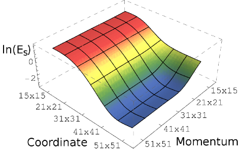
Figure 1: (Color online) Dependence of the $K^{\pi}=1^{+}$ rotational spurious mode on the coordinate and momentum mesh size for the non-linear model NL3 parametrization. For a coordinate and momentum mesh size of (41x41) and (31x31), respectively, the accuracy limit of the diagonalization procedure is achieved. The logarithmic scale in the $z$-axis is used to enhance the readability of the graph. The lowest $z$ value corresponds to a value of around 0.05 MeV.

In normal calculations, because of numerical inaccuracies, truncation of the $ph$-space and inconsistencies among the ground state and RPA equations, the spurious states are often located at energies somewhat higher than zero and often cause a mixing with physical states. There are several approaches to overcome this problem. Some authors adjust a free parameter of the residual interaction until the energy of the spurious mode goes to zero. Another method is to remove a posteriori the spurious components from the physical states by projection. This is possible, because the wave functions of the spurious modes are given by the matrix elements of the corresponding generators RS.80 .

In this investigation a fully self-consistent implementation of the RPA is used, and thus as long as numerical inaccuracies are kept to a minimum, the spurious modes decouple without further complications. Because the block-wise structure of the RPA matrix, they are expected to be present only for specific quantum numbers when specific symmetry constraints are met; since we are restricting to axial symmetry, their expected appearance can be summarized as

• A rotational spurious mode for the $K^{\pi}=1^{+}$ channel associated with rotations of the nucleus as a whole around an axis perpendicular of the symmetry axis in $z$-direction. Its generator is the angular momentum operator $\hat{J}_{+}=\hat{J}_{x}+i\hat{J}_{y}$ Mar.77b .

• A translational spurious mode for the $K^{\pi}=0^{-},1^{-}$ channels associated with the translation of the nucleus as a whole. Its generators are the linear momentum operators $\hat{P}_{z\text{ }}$and $\hat{P}_{+\text{ }}$.

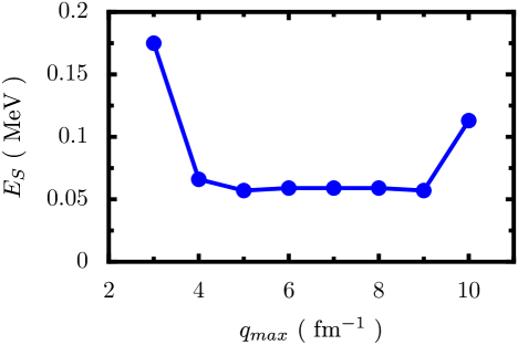
Figure 2: (Color online) Spurious $K^{\pi}=1^{+}$ rotational mode dependence on the maximum interaction momentum while keeping the number of mesh points constant. Good numerical results for a momentum mesh size of (31x31) can be achieved with a maximum momentum in the interval $5<q_{max}<9$.

In fact, the position of the spurious modes provides a very accurate test of the actual numerical implementation of the RMF+RRPA framework. Thus, it is important to study their evolution with the approximations performed. In the present status of the implementation seven parameters control the numerical accuracy, and can be categorized in two groups. The first group specifies the precision of the numerical integrations. In this category are included the number of coordinate and momentum lattice points and the upper boundary of the momentum integrals. The second group deals with the size of the configuration space, and includes the energy cutoffs for $ph$- and $ah$-pairs.

Since it is unfeasible to study this seven-dimensional surface in detail, when studying the dependence of the spurious modes on one, or a set of, parameters, those not under scrutiny were fixed to best possible values the hardware supports. This means, in particular, that the full $ph$ configuration space is taken if not otherwise stated, and that the maximum momentum is fixed to $q_{\max}=8$ fm^-1, well above the Fermi momentum of the nucleus.

In Fig. 1 the position of the rotational $K^{\pi}=1^{+}$ spurious mode in ²⁰Ne is plotted against the number of points in the coordinate and momentum lattices. For a relatively low number of points a plateau is reached where further improvement of the accuracy cannot be achieved. The optimal number of evaluation points for the quadratures is therefore around 41x41, which allows for very precise calculations. Furthermore, additional tests show that the overall precision in the determination of the energy of excited states of the code is capped out at 0.05 MeV, which is surprisingly good.

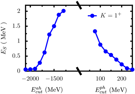
Figure 3: (Color online) On the upper plot we show the dependence of the $K^{\pi}=1^{+}$ rotational spurious mode on the size of the $ph$- and $ah$-space size. The lower plot shows the same dependence for the $K^{\pi}=1^{+}$ and $K^{\pi}=0^{-}$ translational spurious modes.

Figure 2 depicts the position of the rotational $K^{\pi}=1^{+}$ spurious mode for ²⁰Ne against the maximum momentum of the expansion used in the integral for the evaluation of the single particle matrix elements in Eq. (80). The flat region between 5 and 9 fm^-1 hints that a maximum momentum of $q_{\max}=5$ fm^-1 provides enough precision for the proper decoupling of the spurious mode. The increase observed in the position of the spurious mode for maximum momentum values larger than 9 fm^-1 is an artifact due to the number of points for the momentum lattice being fixed at (31x31).

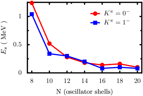
Figure 4: (Color online) Dependence of the $K^{\pi}=1^{-}$ and $K^{\pi}=0^{-}$ translational spurious modes on the configuration space size, dictated by the number of oscillator shells used in the ground-state calculation.

Figure 3 shows the dependence of the rotational $K^{\pi}=1^{+}$ and translational $K^{\pi}=0^{-},1^{-}$ spurious modes on the configuration space size for ²⁰Ne, as calculated with the NL3 parameter set. In the translational case two curves are plotted, one for the $K^{\pi}=0^{-}$ mode and one for the $K^{\pi}=1^{-}$ mode. It is interesting to note that, even if the spurious mode can be brought very close to zero, it requires the inclusion of almost all the possible $ph$-pairs in the configuration space. In this specific case, i.e. in ²⁰Ne, that amounts to the inclusion of roughly five thousand pairs. Several test indicate that the situation improves greatly in heavier nuclei, where usually 5% percent of all possible $ph$-pairs are enough to decouple the spurious modes at energies around 0.5 MeV.

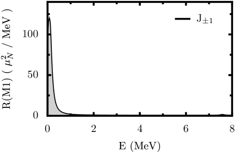
Figure 5: (Color online) Response in ²⁰Ne to the operator $J_{\pm 1}$, generator of rotations around a perpendicular of the symmetry axis. Almost 100% of the strength is exhausted by the spurious mode (situated at 0.08 MeV), with minimal admixture to the physical states.

Since for the solution of the ground-state the equations of motion are expanded in a harmonic oscillator basis, the configuration space where the RPA is solved does not spawn the whole Hilbert space, even if all possible $ph$-pairs are taken. The quality of this expansion depends on the number of major oscillator shells used, and the results obtained at the RPA level will be influenced by this approximation. In particular, the proper decoupling of the translational spurious mode is very sensitive to the number of oscillator shells employed. In Fig. 4 the translational spurious mode is plotted versus the number of oscillator shells used in the ground state. Already with the inclusion of 16 major shells is enough to achieve a precision in the spurious mode of around 0.1 MeV. In all practical cases presented in the this study the number of oscillator shells was chosen between 12 and 16, depending on the desired final precision and the availability of computer resources.

However, more important that the actual position of the spurious modes is their admixture to the real physical states. For the same reasons the spurious mode does not appear at exactly zero energy, the physical states are not completely orthogonal to it, producing unreal results and very often overestimated strength.

Moreover, there is one important property of the spurious modes that can also be used to measure the extent of their admixture with the rest of the RPA states. They are not normalizable in the sense of Eq. (41) because

$$X_{mi}=Y_{mi}$$ (114)

However, in all numerical implementations the relation (114) is only approximately fulfilled because the spurious modes do not decouple exactly. How good the decoupling of the spurious modes is can be measured comparing the relative norms of the different eigen-modes. For an approximate spurious mode labeled as $(sp)$ it should hold that $X_{mi}^{(sp)}\approx Y_{mi}^{(sp)}$, or

$$\delta:=1-\frac{\sum_{mi}|Y_{mi}^{(sp)}|^{2}}{\sum_{mi}|X_{mi}^{(sp)}|^{2}}\ll 1$$ (115)

while for any other RPA mode $\nu$, by initial assumption, it holds that $X_{mi}\gg Y_{mi}$, and thus

$$\delta:=1-\frac{\sum_{mi}|Y_{mi}^{(sp)}|^{2}}{\sum_{mi}|X_{mi}^{(sp)}|^{2}}\approx 1$$ (116)

Our tests indicate that when the spurious modes are located below 0.5 MeV, the value of $\delta$ in Eq. (115) is at least three orders of magnitude smaller than the ones belonging to normal RPA modes. This is a very good indicative of the proper decoupling of the Goldstone modes.

As an example of the low admixture of spurious components with the physical states, Figure 5 shows the response to the generator of the rotational spurious mode, the operator $J_{\pm 1}$, which represents rotations around an axis perpendicular to the symmetry axis. More than 99.99% of the strength is exhausted by the spurious mode, which is located below 0.1 MeV. Similar results are obtained for the translational spurious modes in ²⁰Ne.

In general, it was observed that, if the position of the spurious mode is below 1 MeV, the strength function of the rest of the spectrum is mostly unaffected. The spectrum in the low energy region, below 5 MeV, is, however, more sensitive to admixtures of the spurious modes; as a rule of thumb, the confidence limit in the position of the spurious mode, for a proper decoupling, has been consistently found around 0.5 MeV.

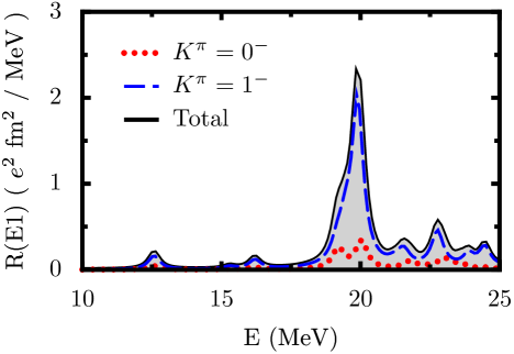
Figure 6: (Color online) $K^{\pi}=0^{-}$ and $K^{\pi}=1^{-}$ response to the E1 transition operator for the spherical nucleus ¹⁶O.

There is still another test that can be devised in order to check the consistency of the whole framework, namely the conservation of spherical symmetry. Even though all the formulas are particularized to the case of axial symmetry, the interaction is rotationally invariant, so they should still be valid when a spherical ground-state is taken as basis for the RPA configuration space, i.e., they should preserve spherical symmetry.

In Figure 6 is plotted the E1 excitation strength for the spherical nucleus ¹⁶O. Since the E1 operator is a rank-one tensor, it has three possible angular momentum projections, $K=-1,0,1$, that have to be calculated separately. The response for the modes with $K=-1$ and $K=1$ are identical and correspond to vibrations perpendicular to the symmetry axis, i.e. one can calculate only one of them and double its contribution. The $K=0$ mode corresponds to vibrations along the symmetry axis. If the nucleus is prolate, like ²⁰Ne, the response for in the $K=0$ mode should lie at lower energies than the $K=1$ mode, as the potential is flatter in the direction of the symmetry axis. However, if the nucleus is spherical, like ¹⁶O, there is no distinction between the $K=0$ and $K=1$ modes, and their corresponding excitation strength should lie at exactly the same energies. From Figure 6 one can attest that the procedure for the solution of the RPA equation in axial symmetry indeed preserves rotational symmetry with a good degree of accuracy.

The study presented concerning the decoupling of the spurious modes and the preservation of spherical symmetry shows that the numerical implementation solves the equations posed by the self-consistent RMF+RPA framework in axial symmetry. We have also ascertained that a high degree of accuracy can be achieved in real calculations, as well as validated the good reproduction of formal and mathematical aspects of the RPA theory.

VII Applications in ²⁰Ne

As a first application of the RMF+RRPA framework we have undertaken a model study of the magnetic and the electric dipole response in ²⁰Ne. This nucleus offers several advantages. Its ground state is well deformed and exhibits a prolate shape in the RMF model, with a quadrupole deformation parameter $\beta\approx 0.5$. Another advantage is the reduced number of nucleons to be taken into account in the calculations, which translates in fast running times and thus in the possibility of detailed analysis. With the optimal number of oscillator shells for a ground state calculation with full precision, the number of pairs never exceeds five thousand. Furthermore, because the number of protons and neutrons is the same, switching off the electromagnetic interaction should give identical results for both protons and neutrons. Using this technique, very detailed checks can be carried out on the isospin part of the interaction, and its consistency can be further established. All these reasons make ²⁰Ne the ideal theoretical playground where to introduce the concepts that can later be used in the study of more complex systems. In the this section we shall present two sample applications for the well deformed nucleus ²⁰Ne.

VII.1 The magnetic dipole (M1) response

We first consider the magnetic dipole response. The discovery of low-lying M1 excitations, known as scissors mode, was made by Richter and collaborators in ¹⁵⁶Gd in Darmstadt through a high-resolution inelastic electron scattering experiment BRS.84 . The search for such a mode was stimulated by the theoretical prediction of a collective mode, where the deformed proton distribution oscillates in a rotational motion against the deformed neutron distribution SR.77 ; IP.78a ; IP.78b ; Hil.84 ; Hil.92 . The name “scissors mode” was indeed suggested by such a geometrical picture. An excitation of similar nature was also predicted by group-theoretical models Iac.81 ; Die.83 ; Iac.84 .

The mode has been detected in most of the deformed nuclei ranging from the $fp$-shell to rare-earth and actinide regions. The mode has been well characterized, and it is established that it is fragmented over several closely packed M1 excitations. For reviews to this mode and for recent semiclassical investigations see Refs. VHJ.86 ; KPZ.96 ; Rich.95 ; Zaw.98 ; BalS.07a ; BalS.07b

A byproduct of the systematic study of the scissors mode was the discovery of spin excitations. Inelastic proton scattering experiments on ¹⁵⁴Sm and other deformed nuclei found a sizable and strongly fragmented M1 spin strength distributed over an energy range of 4-12 MeV FWR.90 . The experimental discovery stimulated theoretical investigations in the RPA approximation HHR.98 .

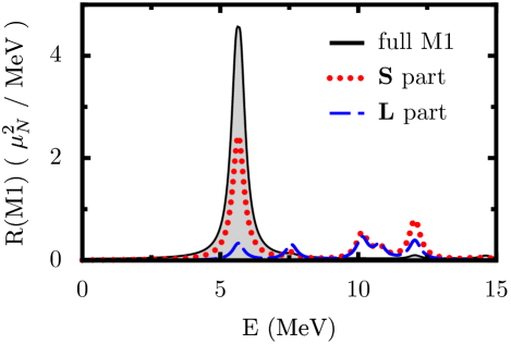
Figure 7: (Color online) M1 Excitation strength for ²⁰Ne, using the NL3 parameter set. A very well developed peak can be seen around 5.8 MeV. Its structure is composed mostly of spin flip transitions.

Figure 7 shows the response to the M1 magnetic dipole operator in the nucleus ²⁰Ne . The shaded region corresponds to the full M1 response; the blue dashed line is the response to orbital part of the M1 operator and the red dotted line refers to the spin part. The calculations were performed with the maximum precision allowed by the current implementation of the computer code. The number of pairs is around five thousand. Optimal numerical parameters were chosen in order to minimize the error. The rotational spurious mode is well separated, situated around 0.1 MeV, i.e. no admixture with the vibrational response is observed.

Only one prominent peak is found around 5.7 MeV. Regrettably, there is no experimental data available for the magnetic response in this nucleus. Theoretical studies using large scale shell model calculations CP.86 predict a low lying orbital mode around 11 MeV for ²⁰Ne, in strong disagreement with our results. However, other calculations LZ.87 performed in ²²Ne, with the same shell model interaction, exhibit two dominant low lying peaks around 5-6 MeV. The orbital contribution to the total response is below 25%, which is in better agreement with results found within our RMF+RRPA calculations, where fragmented strength with similar characteristics is found in the same energy region.

Regarding the contributions from the orbital and spin components of the M1 operator to the total response, it can be observed in Figure 7 that there are two differentiated energy regions. Around the main excitation peak at 6 MeV there is an enhancement of the response due to the additive interference of the orbital and spin contributions. In contrast, in the energy region above 6.5 MeV we observe the opposite, destructive interference and both contributions cancel. This feature of the M1 strength distribution has been also found in other studies HHR.98 and is much more evident in the case of heavier nuclei.

From this figure we can also recognize that the main contribution to the total response comes from spin excitations. The supposed orbital character of the low lying spectra in the M1 transitions is eclipsed by the preponderance of spin flip strength, three times larger than the orbital response. Again, this is in disagreement with the cited shell model calculation CP.86 , which in ²⁰Ne predicts a much bigger orbital contribution to the total strength. However, low lying collective transitions in such a light nucleus as ²⁰Ne cannot be expected to be exceptionally well described by the RMF+RRPA theory. In few nucleon systems, the single particle structure around the Fermi surface is of the utmost importance in the calculation of low-lying excitations. As such, the results produced in a self-consistent mean field calculation are not so reliable. A better description would require a proper account of excitations to the continuum above the coulomb barrier and probably for higher order correlations at the time dependent mean field level. The situation improves in heavier nuclei, were mean field theories were designed to yield good results at low computational costs.

Peak at 5.7 MeV
					$\varepsilon_{1}-\varepsilon_{2}$
P	49%	$\frac{1}{2}^{+}[220]$	$-$	$\frac{3}{2}^{+}[211]$	5.15
N	48%	$\frac{1}{2}^{+}[220]$	$-$	$\frac{3}{2}^{+}[211]$	5.22
P	1%	$\frac{1}{2}^{+}[220]$	$-$	$\frac{1}{2}^{+}[211]$	9.73
N	0.9%	$\frac{1}{2}^{+}[220]$	$-$	$\frac{1}{2}^{+}[211]$	10.17

Table 1: $ph$ structure for the 5.7 MeV M1 transition mode in ²⁰Ne for the NL3. The second column refers to the normalization of the RPA amplitudes. The level quantum numbers in the third column are $\pm\Omega^{\pi}$, where $\pm\Omega$ is the angular momentum projection over the symmetry axis and $\pi$ is the parity. In square brackets are the quantum numbers of the oscillator state which contributes most to the mean field single particle level. The effect of coulomb interaction can be seen as the small differences in the mixing percentages for protons and neutrons. A calculation with the electromagnetic interaction switched off gives as a result a perfect isospin symmetry, with no differences observable within the accuracy of the computed results.

Nevertheless, it is still interesting to delve further into the study of the properties of the main excitation peak, as the same analysis can be performed in heavier nuclei and many of the general features will still be present. The study of the structure of the excitation peaks can be carried out in detail attending to their $ph$ structure. The contribution $C_{ph}$ from a particular proton or neutron $ph$ configuration to a RPA state is determined by

$$C_{ph}=(|X_{ph}^{\nu}|^{2}-|Y_{ph}^{\nu}|^{2})$$ (117)

where $X^{\nu}$ and $Y^{\nu}$ are the RRPA amplitudes associated with a particular excitation energy. Table 1 outlines the single particle decomposition of the dominant M1 peak observed in Figure 7. All the strength is provided by a single particle transition within the sd-shell, from the last level in the Fermi sea to the first consecutive unoccupied level. The low collectivity indicates that, within the RMF+RRPA model, the spectrum of the M1 operator in ²⁰Ne is of single particle character. Each of the two Dirac spinors in the particle-hole pair corresponds to a eigen state of the static RMF potential. They can be characterized by the Nilsson quantum numbers $\Omega^{\pi}[Nn_{z}\Lambda]$ of their largest component in an expansion in anisotropic oscillator wave functions. Here $\Omega$ is total angular momentum projection onto the symmetry axis, $\pi$ is the parity, $N=2n_{r}+n_{z}+\Lambda$ is the major oscillator quantum number, and $\Lambda=\Omega-m_{s}$ is the projection of the orbital angular momentum on to the symmetry axis. From these quantum numbers one concludes the following approximate selection rules: $\Delta\Omega=+1$, $\Delta N=0$, $\Delta n_{z}=-1$ and $\Delta\Lambda=+1$. The orbital character of the excitation peak is confirmed by the fact that $\Delta\Omega=\Delta\Lambda$, which implies that the change in the magnetic quantum number $m_{s}$ is zero. It is interesting to note that even if the approximate selection rule points to an orbital character for the mode, the spin strength is nevertheless dominant.

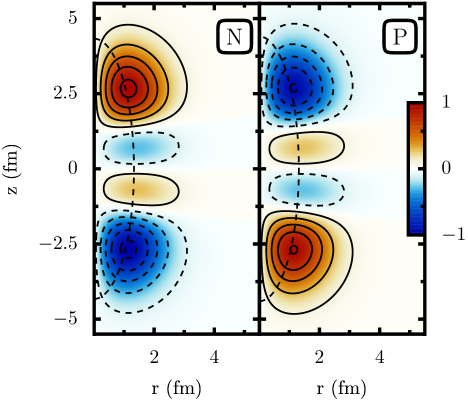
Figure 8: (Color online) Intrinsic transition density for neutrons (left) and protons (right) of the M1 peak at 5.7 MeV in in ²⁰Ne. Full (red shade) and dashed lines (blue shade) indicate positive and negative values, respectively. The $z$-coordinate runs along the symmetry axis and $r$ is the distance from the symmetry axis. The thin dotted line represents the rms radius of the ground state neutron or proton density, and qualitatively marks the position of the ground state nuclear surface.

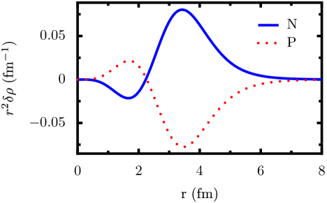
Figure 9: (Color online) Radial part of the projected (to $I=1$, $M=1$) transition densities of the M1 peak at 5.7 MeV. $r$ is the distance from the symmetry axis. The prominent isovector nature is patent in the graphs.

It is difficult to form a geometrical image of the nature of an excitation, having at hand only the information given in Table 1. For that purpose, it is always useful to compare the the neutron and proton intrinsic transition densities in a plot. Figure 8 shows a color plot of the transition densities at an excitation energy of 5.7 MeV. Color is used to indicate the value of the function, with blue for negative values and red for positive ones. Regions with the same kind of line (solid or dashed), or color shade (red or blue), for both protons and neutrons are indicative of an in-phase vibration, while in regions where the opposite is true protons and neutrons vibrate out-of-phase. In this case the excitation is of clear isovector nature, and we can observe the typical structure of a scissors mode; neutrons and protons are out of phase over the full space, with a concentration near the caps of the prolate nuclear shape.

In such a simple case as the one found in ²⁰Ne the interpretation of the two dimensional color plot for the transition densities is very clear. They represent the intrinsic transition densities, referred to the intrinsic frame of reference, where only the total angular momentum projection on the symmetry axis is well defined. In that regard, they are expected to contain admixtures from all possible angular momenta. However, the transition operator (M1 in this specific case) restricts the major contributions of the transition densities to the total response to its own total angular momentum, i.e. to in the case of M1 transitions to $I=1$. It is therefore advisable to project out the weaker-contributing angular parts from the densities to obtain the actual transition density that would be observed in the laboratory frame of reference. For the M1 operator that means retaining , with the help of Eq. (113) only the contributions coming from angular momentum $I=1$. In Figure 9 the radial part of such a projected transition density is plotted for the main peak in the ²⁰Ne M1 response.

Both transition densities are almost the mirror of each other, a very clear indication of the pure isovector nature of the mode at 5.7 MeV. We have already seen that in simple geometrical terms this mode can be interpreted as a rotation of neutrons against protons around an axis perpendicular of the symmetry axis. Furthermore, details in Figure 8 show that two distinct regions can be distinguished. They are separated at around 2 fm from the origin, where the direction of rotation for protons and neutrons changes. The appearance of two regions (as depicted in Figure 9) is already a strong hint that the simple picture of the proton density rotating against the neutron density as rigid rotors (as in the Two Rotor Model IP.78a ) does not reflect reality in this nucleus. The traditional scissors picture considers the neutron and proton densities as the blades of a scissor oscillating against each other. In addition, one has to take into account the angular momentum inherent in a $K=1^{+}$ excitation: it can be descibed as an oscillation of the scissor which rotates at the same time rotating slowly around its longitudinal symmetry axis. However, the picture we derive from the results of our calculation is somewhat different.

VII.2 The Electric dipole (E1) response

We have chosen the electric dipole response in ²⁰Ne as a second example application of the RMF+RRPA formalism with axial symmetry. In Fig. 10 the E1 strength is plotted as calculated with the NL3 parameter set. The red curve corresponds to excitations along the symmetry axis with $K^{\pi}=0^{-}$, while the blue curve are those perpendicular to the symmetry axis with $K^{\pi}=1^{-}$. In principle, for prolate nuclei, as is the case for ²⁰Ne, the strength due to the $K^{\pi}=0^{-}$ mode should lie at lower energies compared to the $K^{\pi}=1^{-}$ mode. As the nuclear potential must be flatter (more extended) along the symmetry axis, it is energetically more favorable for the nucleons to oscillate in that direction than along an axis perpendicular to the symmetry axis, where the nuclear potential is narrower. It is possible, therefore, to relate the nuclear deformation with the energy separation of the two modes Dan.58 ; Oka.58 .

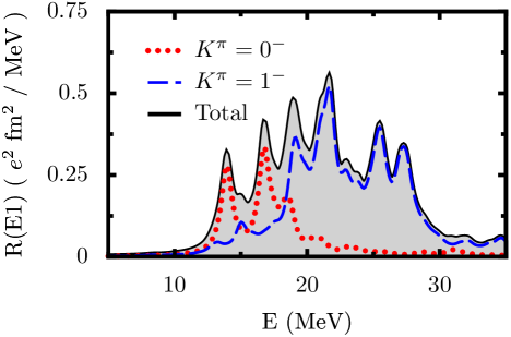
Figure 10: (Color online) E1 strength in ²⁰Ne, as calculated with the NL3 parameter set.

The splitting of the response due to the broken spherical symmetry, and its interpretation, can be observed in Figures 11 and 12. The former is the transition density for the main IVGDR peak at 16.73 MeV observed in the $K^{\pi}=0^{-}$ response, while the latter corresponds to the peak at 21.31 MeV in the $K^{\pi}=1^{-}$ mode. The prolate deformation is evident, as the intrinsic transition densities are elongated in the direction of the $z$-axis. The character of the $K^{\pi}=1^{-}$ mode as a vibration along a perpendicular of the symmetry axis is easily recognizable in Figure 12. By comparison, the transition density in Figure 11 is then easily interpreted as a vibration along the symmetry axis. As it is expected for the IVGDR, the neutron-proton vibrations are out of phase over the same spatial regions. It is more evident still looking at their respective projections to the laboratory system of reference, which are shown in the lower plots of Figures 11 and 12.

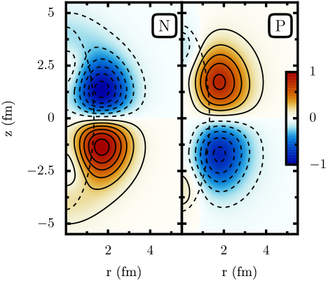
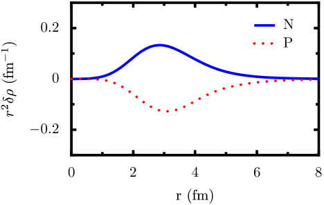
Figure 11: (Color online) ²⁰Ne IVGDR transition density for the $K^{\pi}=0^{-}$ peak at 16.7 MeV, NL3 parameter set.

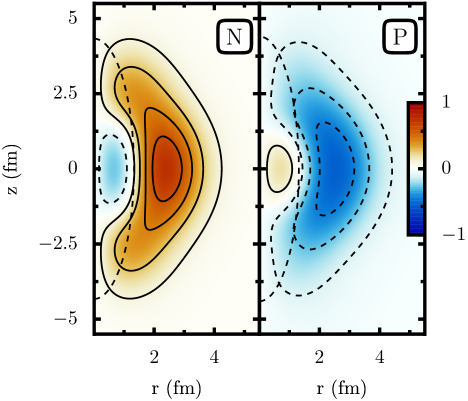
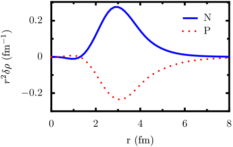
Figure 12: (Color online) ²⁰Ne IVGDR transition density for the $K^{\pi}=1^{-}$ peak at 21.3 MeV, NL3 parameter set.

Coming back to Figure 10, the response in the energy region between 15 MeV and 25 MeV corresponds to the IVGDR. Its strength is heavily fragmented into several peaks in an energy interval of about 3-4 MeV for both excitation modes. The main contributions to the strength curve come from more than four different peaks. For example, the $K^{\pi}=1^{-}$ IVGDR response is composed, besides the already mentioned peak at 21.3 MeV, by four additional major peaks, situated at 19.6, 20.2, 21.8, and 22.4 MeV respectively. Their projected transition densities, in Figure 13, show that all of them can be classified as a vibration of the neutron density against the proton density.

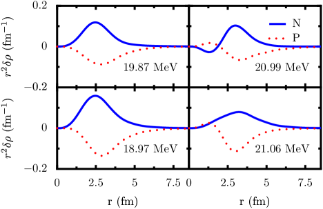
Figure 13: (Color online) Projected transition densities for major $K^{\pi}=1^{-}$ peaks contributing to the electric dipole response in ²⁰Ne.

The decomposition in $ph$ components of the main $K^{\pi}=0^{-}$ and $K^{\pi}=1^{-}$ IVGDR peaks can be found in Table 2. The characteristic $\Delta N=1$ pattern of the IVGDR is present in both peaks. The high collectivity indicates a very coherent excitation pattern that fits into the properties of a giant resonance. This phenomenon can also be observed in the transition densities, where the coherent superposition of $ph$ pairs is evident in the absence of wavefunction-like features, and is easily interpreted in a macroscopic picture where the proton and neutron densities oscillate one against the other. The total percentage of the classical TRK sum-rule exhausted between 10 MeV and 40 MeV for the calculated E1 response in ²⁰Ne is 111%. In a fully classical system the share of the strength exhausted by the $K^{\pi}=1^{-}$ mode should be double than that exhausted by the $K^{\pi}=0^{-}$ mode; however, with 86% of the TRK sum-rule coming from the $K^{\pi}=1^{-}$ mode and 25% from the $K^{\pi}=0^{-}$ mode, it is obvious that it is no longer true for quantum systems, even though we do not fully understand the mechanism behind this phenomenon.

$K^{\pi}=0^{-}$ peak at 16.73 MeV
					$\varepsilon_{1}-\varepsilon_{2}$
N	20%	$\frac{3}{2}^{-}[101]$	$-$	$\frac{3}{2}^{+}[211]$	14.25
P	18%	$\frac{3}{2}^{-}[101]$	$-$	$\frac{3}{2}^{+}[211]$	13.89
N	16%	$\frac{1}{2}^{+}[220]$	$-$	$\frac{1}{2}^{-}[321]$	17.52
N	11%	$\frac{1}{2}^{-}[101]$	$-$	$\frac{1}{2}^{+}[200]$	15.28
P	9%	$\frac{1}{2}^{-}[101]$	$-$	$\frac{1}{2}^{+}[211]$	14.46
N	7%	$\frac{1}{2}^{+}[220]$	$-$	$\frac{1}{2}^{-}[310]$	18.20
P	5%	$\frac{1}{2}^{-}[101]$	$-$	$\frac{1}{2}^{+}[211]$	12.71
N	3%	$\frac{1}{2}^{-}[101]$	$-$	$\frac{1}{2}^{+}[211]$	13.37
N	2%	$\frac{1}{2}^{+}[220]$	$-$	$\frac{1}{2}^{-}[330]$	12.90
$K^{\pi}=1^{-}$ peak at 21.31 MeV
					$\varepsilon_{1}-\varepsilon_{2}$
N	13%	$\frac{1}{2}^{-}[110]$	$-$	$\frac{3}{2}^{+}[211]$	20.01
N	13%	$\frac{1}{2}^{+}[220]$	$-$	$\frac{1}{2}^{-}[321]$	20.64
P	11%	$\frac{1}{2}^{+}[220]$	$-$	$\frac{1}{2}^{-}[321]$	22.03
P	9%	$\frac{1}{2}^{-}[101]$	$-$	$\frac{1}{2}^{+}[200]$	21.55
N	7%	$\frac{1}{2}^{-}[110]$	$-$	$\frac{1}{2}^{+}[211]$	24.96
P	5%	$\frac{1}{2}^{-}[101]$	$-$	$\frac{3}{2}^{+}[202]$	22.83
N	5%	$\frac{1}{2}^{+}[220]$	$-$	$\frac{1}{2}^{-}[321]$	23.81
N	5%	$\frac{1}{2}^{+}[220]$	$-$	$\frac{3}{2}^{-}[312]$	21.56
N	4%	$\frac{1}{2}^{+}[220]$	$-$	$\frac{3}{2}^{-}[321]$	22.79

Table 2: Particle-hole structure of the two main IVGDR modes. N and P indicate a neutron or proton $ph$ pair, respectively. The second column is the percentage of the contribution of each particular $ph$ excitation. The Nilsson quantum numbers, labeling the particle-hole, are shown in the next columns. The last column gives the energy of the excitation in MeV.

VIII Concluding remarks

In the present investigation we have formulated the relativistic random phase approximation (RRPA) on the basis of a relativistic mean-field (RMF) model having axial symmetry in a fully self-consistent way, i.e., the interactions used in both the RMF equations and in the matrix equation of the RRPA are derived from the same Lagrangian, i.e. the same energy functional. As it has been shown, this self-consistency feature is of vital importance for the fulfillment of current conservation and the proper decoupling of spurious modes without further adjustments in the interaction.

So far, pairing correlations have not been included. The inclusion of such correlations will allow the application of this method to a large number of investigations in medium and heavy nuclei, in particular, in a first step, for a systematic study of low-lying electric and magnetic dipole strength over large regions of the periodic table. Of course, the study of the nuclear response to other electric and magnetic multipoles is also open to scrutiny. Since the formulation of relativistic proton-neutron RPA, once the main building blocks presented in this document are present, is mostly trivial, its implementation opens the door to the wide area of nuclear spin-isospin excitations, in particular the Isobaric Analog Resonance (IAR) and the Gamov-Teller Resonance (GTR), but also for many types of weak processes such as the $\beta$-decay and neutrino-reactions in deformed nuclei.

In conclusion, the relativistic RPA formulated for axially deformed systems represents a significant new theoretical tool for a realistic description of excitation phenomena in large regions of the nuclear chart, which has been accessible so far only by relatively crude phenomenological models. Its development, and the sample application presented in this document, show that its future use in nuclear structure and astrophysics will provide an valuable insight into very important, and still open, questions about the nature of nuclear interaction, collective response, deformation effects and cross sections relevant for astrophysical processes.

Appendix A Two-body matrix elements

Starting form the general expression for the two-body matrix element in Eq. (79)

$$\langle kl^{\prime}|\hat{V}_{m}^{ph}|k^{\prime}l\rangle=\int\frac{d^{3}q}{(2\pi)^{3}}\langle k|\hat{Q}^{\mu}(\boldsymbol{q})|k^{\prime}\rangle\Delta_{m}(\boldsymbol{q})\langle l|\hat{Q}_{\mu}(\boldsymbol{q})|l^{\prime}\rangle^{\ast}$$ (118)

we first have to evalute the matrix elements (80) for the single particle opreators $Q^{\mu}(\boldsymbol{q}).$ In cylindrical coordinates

$$\boldsymbol{q}=(q_{x},q_{y},q_{z})=(q\cos\chi,q\sin\chi,q_{z})$$ (119)

we obtain

$$Q_{kk^{\prime}}^{\mu}(q,\chi,q_{z})=\int\frac{d\varphi}{2\pi}\,d^{2}r\,~{}\bar{\psi}_{k}g_{m}\,\Gamma^{\mu}\,\psi_{k^{\prime}}\,e^{iq_{z}z+iqr\cos(\varphi-\chi)}$$ (120)

It turns out to be useful to  classify the various vertices $\Gamma^{\mu}$ by the spin quantum numbers $S$ and $S_{z}=\Sigma$ of the exchanged meson. For this reason we use the the $\gamma$-matrices in the Dirac basis defined by

$$\{\gamma^{0},\gamma^{+}=\frac{-1}{\sqrt{2}}(\gamma^{1}+i\gamma^{2}),\gamma^{-}=\frac{1}{\sqrt{2}}(\gamma^{1}-i\gamma^{2}),\gamma^{3}\}$$ (121)

and obtain

$$\gamma^{\mu}\gamma_{\mu}=\gamma^{0}\gamma^{0}+\gamma^{+}\gamma^{-}+\gamma^{-}\gamma^{+}-\gamma^{3}\gamma^{3}$$ (122)

Including the scalar mesons (and neglecting for the moment the isospin) we therefore have 5 vertices characterized by the index $\tilde{\mu}$:

$$\Gamma^{\tilde{\mu}}=(1,\gamma^{0},\gamma^{+},\gamma^{-},\gamma^{3}).$$ (123)

$\tilde{\mu}$ runs over $\tilde{\mu}=s$ (for scaler mesons, $S=\Sigma=0$), $\tilde{\mu}=0$ (for the time-like part of the vector mesons, $S=\Sigma=0$) and $\tilde{\mu}=+,-,3$ (for the spatial parts of the vector mesons with $S=1$). The channels $\tilde{\mu}=\pm$ describe the spin flip ($\Sigma=\pm 1$) and $\tilde{\mu}=3$ has $\Sigma=0$.

Using the Dirac spinors in cylindrical coordinates (65) and exploiting the properties of the $\gamma$-matrices defined in Eq. (121), we find that the $\varphi$-dependence of the amplitudes $\bar{\psi}_{k}(r,\varphi,z)\,\Gamma^{\tilde{\mu}}\,\psi_{k^{\prime}}(r,\varphi,z)$ can be separated

$$\bar{\psi}_{k}(r,\varphi,z)\,\Gamma^{\tilde{\mu}}\,\psi_{k^{\prime}}(r,\varphi,z)=i^{S}\,F_{kk^{\prime}}^{\tilde{\mu}}(r,z)e^{i\Lambda\varphi}$$ (124)

where the integer

$$\Lambda=\Omega_{k}-\Omega_{k^{\prime}}-\Sigma=K-\Sigma$$ (125)

is the orbital part of the angular momentum of the pair in $z$-direction. The real functions $F_{kk^{\prime}}^{\tilde{\mu}}(r,z)$ are given by

$$F_{kk^{\prime}}^{s}(r,z) =f_{k}^{+}f_{k^{\prime}}^{+}+f_{k}^{-}f_{k^{\prime}}^{-}-g_{k}^{+}g_{k^{\prime}}^{+}-g_{k}^{-}g_{k^{\prime}}^{-},$$ (126)

$$F_{kk^{\prime}}^{0}(r,z) =f_{k}^{+}f_{k^{\prime}}^{+}+f_{k}^{-}f_{k^{\prime}}^{-}+g_{k}^{+}g_{k^{\prime}}^{+}+g_{k}^{-}g_{k^{\prime}}^{-},$$ (127)

$$F_{kk^{\prime}}^{+}(r,z) =g_{k}^{+}f_{k^{\prime}}^{-}-f_{k}^{+}g_{k^{\prime}}^{-}$$ (128)

$$F_{kk^{\prime}}^{-}(r,z) =f_{k}^{-}g_{k^{\prime}}^{+}-g_{k}^{-}f_{k^{\prime}}^{+}$$ (129)

$$F_{kk^{\prime}}^{3}(r,z) =f_{k}^{+}g_{k^{\prime}}^{+}-g_{k}^{+}f_{k^{\prime}}^{+}+f_{k}^{-}g_{k^{\prime}}^{-}-g_{k}^{-}f_{k^{\prime}}^{-}$$ (130)

This allows us to evaluate the $\varphi$-integration in the integral (120) analytically and to express it in terms of Bessel functions of the first kind

$$J_{n}(x)=(-i)^{n}\int_{0}^{2\pi}\frac{d\varphi}{2\pi}\,e^{in\varphi}e^{ix\cos\varphi}.$$ (131)

We obtain

$$\mathrm{Q}_{kk^{\prime}}^{\tilde{\mu}}(\boldsymbol{q})=i^{\Lambda+S}\,e^{i\Lambda\chi}\,\mathcal{F}_{kk^{\prime}}^{\tilde{\mu}}(q,q_{z})$$ (132)

with the integrals

$$\mathcal{F}_{kk^{\prime}}^{\tilde{\mu}}(q,q_{z})={\displaystyle\int}\,d^{2}r\,\,F_{kk^{\prime}}^{\tilde{\mu}}(r,z)\,J_{\Lambda}(qr)\,e^{iq_{z}z}.$$ (133)

which are either real or purely imaginary. Using the parity relation

$$F_{kk^{\prime}}^{\tilde{\mu}}(r,-z)=\pi(-)^{S+\Lambda}F_{kk^{\prime}}^{\tilde{\mu}}(r,z)$$ (134)

whe recognize that the exponential factor $e^{iq_{z}z}$ reduces to the cosine or sine depending of the quantum numbers $\pi$ and $K$ of the mode and on the spin quantum numbers $S,\Sigma$ of the vertex $\tilde{\mu}$

$$e^{iq_{z}z}\rightarrow\left\{\begin{array}[c]{c}~{}\cos(q_{z}z)\text{ \ for \ \ }\pi(-)^{K+S-\Sigma}=+1\\ i\sin(q_{z}z)\text{ \ \ }\mathrm{for}\text{ \ \ }\pi(-)^{K+S-\Sigma}=-1\end{array}\right.$$ (135)

Substitution of these expressions in the integral of Eq. (118) the $\chi$-integration can be carried out analytically and leads to the selection rule

$$\Omega_{k}-\Omega_{k^{\prime}}=\Omega_{l}-\Omega_{l^{\prime}}.$$ (136)

and to the following matrix elements for the exchange of scalar mesons

$$\left\langle kl^{\prime}|\hat{V}_{\sigma}^{ph}|k^{\prime}l\right\rangle=-\int\frac{d^{2}q}{(2\pi)^{2}}\mathcal{F}_{kk^{\prime}}^{s}\Delta_{\sigma}\mathcal{F}_{ll^{\prime}}^{s\ast},$$ (137)

of time-like part vector mesons

$$\left\langle kl^{\prime}|\hat{V}_{\omega^{0}}^{ph}|k^{\prime}l\right\rangle=+\int\frac{d^{2}q}{(2\pi)^{2}}\mathcal{F}_{kk^{\prime}}^{0}\Delta_{\omega}\mathcal{F}_{ll^{\prime}}^{0\ast},$$ (138)

and of space-like of the vector mesons

$$\left\langle kl^{\prime}|\hat{V}_{\mathbf{\omega}}^{ph}|k^{\prime}l\right\rangle =\int\frac{d^{2}q}{(2\pi)^{2}}\mathcal{F}_{kk^{\prime}}^{+}\Delta_{\omega}\mathcal{F}_{ll^{\prime}}^{-\ast}$$ (139)

$$+\int\frac{d^{2}q}{(2\pi)^{2}}\mathcal{F}_{kk^{\prime}}^{-}\Delta_{\omega}\mathcal{F}_{ll^{\prime}}^{+\ast}$$ (140)

$$-\int\frac{d^{2}q}{(2\pi)^{2}}\mathcal{F}_{kk^{\prime}}^{3}\Delta_{\omega}\mathcal{F}_{ll^{\prime}}^{3\ast},$$ (141)

where, for simplicity, we have neglected for each matrix element a factor $\delta_{\Omega_{k}-\Omega_{k^{\prime}},\Omega_{l}-\Omega_{l^{\prime}}}$ and the arguments in the functions $\mathcal{F}_{kk^{\prime}}^{\tilde{\mu}}(q,q_{z})$ and in the propagators

$$\Delta_{m}(q,q_{z})=\frac{1}{q^{2}+q_{z}^{2}+m_{m}^{2}}.$$ (142)

in the two-dimensional momentum integrals.

Appendix B Non-linear $\sigma$ propagator in momentum space

The equation to solve is

$$[-\Delta+m_{\sigma}^{2}+W(\boldsymbol{r})]\delta\sigma(\boldsymbol{r})=-g_{\sigma}\delta\rho_{\text{s}}(\boldsymbol{r})$$ (143)

with

$$W(\boldsymbol{r})=2g_{2}\sigma+3g_{3}\sigma^{2}$$ (144)

Because of axial symmetry and using cylindrical coordinates $\boldsymbol{r=}(r\cos\varphi,r\sin\varphi,z)$ $W(\boldsymbol{r}):=W(r,z)$ does not depend on the azimuth angle $\varphi$. We solve Eq. (143) in momentum space. $W(\boldsymbol{r})$ is local in $r$-space, but it is an operator in momentum space

$$W(\boldsymbol{q},\boldsymbol{q}^{\prime})={\displaystyle\int}d^{3}rW(\boldsymbol{r})e^{-i\boldsymbol{r}(\boldsymbol{q}-\boldsymbol{q}^{\prime})}$$ (145)

The propagator in momentum space is the solution of

$$(\boldsymbol{q}^{2}+m^{2})\Delta(\boldsymbol{q},\boldsymbol{q}^{\prime})+{\displaystyle\int}d^{3}rW(\boldsymbol{q},\boldsymbol{q}^{\prime\prime})\Delta(\boldsymbol{q}^{\prime\prime},\boldsymbol{q}^{\prime})=\delta(\boldsymbol{q}-\boldsymbol{q}^{\prime})$$ (146)

where the $\ast$ is the convolution operator and $W(\boldsymbol{q})$ is the Fourier transform of $W(\boldsymbol{r})$. Expanding the $\delta$-function in cylindrical coordinates in $q$-space using $\boldsymbol{q=}(q\cos\chi,q\sin\chi,q_{z})$ we find

$$\delta(\boldsymbol{q}-\boldsymbol{q}^{\prime})=\frac{\delta(q-q^{\prime})}{q}\delta(q_{z}-q_{z}^{\prime})\sum_{n=-\infty}^{\infty}e^{in(\chi-\chi^{\prime})}$$ (147)

and taking the following ansatz for $\Delta$

$$\Delta(\boldsymbol{q},\boldsymbol{q}^{\prime})=\sum_{n=-\infty}^{\infty}\Delta_{n}(q,q_{z},q^{\prime},q_{z}^{\prime})\;e^{in(\chi-\chi^{\prime})}$$ (148)

and inserting it in Eq. (146) leads to a set of integral equations for each $\Delta_{n}$

$$(q^{2}+q_{z}^{2}+m^{2})\Delta_{n}(q,q_{z},q^{\prime},q_{z}^{\prime})$$

$$+\int d^{2}q^{\prime\prime}W_{n}(q,q_{z},q^{\prime\prime},q_{z}^{\prime\prime})\Delta_{n}(q^{\prime\prime},q_{z}^{\prime\prime},q^{\prime},q_{z}^{\prime})$$

$$=\frac{\delta(q-q^{\prime})}{q}\delta(q_{z}-q_{z}^{\prime}),$$ (149)

where we have used the obvious notation $d^{2}q=qdqdq_{z}$. Each $W_{n}$ can be calculated using the following series expansion

$$e^{\mathrm{i}xcos(\alpha)}=\sum_{n=-\infty}^{\infty}\mathrm{i}^{n}J_{n}(x)e^{\mathrm{i}n\alpha}$$ (150)

that leads to the following expression for the non-linear $\sigma$ field in momentum space

$$W_{n}(q,q_{z},q^{\prime},q_{z}^{\prime})=\int\frac{d^{2}r}{2\pi}W(r,z)e^{-i(q_{z}-q_{z}^{\prime})z}J_{n}(qr)J_{n}(q^{\prime}r)$$

that together with Eq. 149 allow the numerical evaluation of the non-linear $\sigma$ propagator in momentum space.

Appendix C Evaluation of the M1 single particle matrix elements

The M1 operator is defined as:

$$\hat{M}_{1\mu}=\sqrt{\frac{3}{4\pi}}\mu_{N}\left(g_{s}\boldsymbol{s}+g_{l}\boldsymbol{l}\right)$$ (151)

with

$$\begin{array}[c]{ccc}g_{s}&=&g_{p}\\ g_{l}&=&1\end{array}\}\quad\mathrm{protons}\qquad\begin{array}[c]{ccc}g_{s}&=&g_{n}\\ g_{l}&=&0\end{array}\}\quad\mathrm{neutrons}$$ (152)

In the spherical coordinates defined as:

$$x_{+}=\frac{-1}{\sqrt{2}}\left(x+iy\right),\text{ \ \ }x_{-}=\frac{1}{\sqrt{2}}\left(x-iy\right),\text{ \ \ }x_{0}=z$$ (153)

we find

$$s_{+} =\frac{1}{2}\Sigma_{+}=\frac{-1}{2\sqrt{2}}\left(\Sigma_{x}+i\Sigma_{y}\right)$$ (154)

$$l_{+} =\frac{\mathds{1}}{2\sqrt{2}}e^{i\varphi}\left[r\partial_{z}-z\left(\partial_{r}+i\frac{1}{r}\partial_{\varphi}\right)\right]$$ (155)

and in the $\hat{M}_{11}$ single particle matrix elements the integration over the azimuthal angle $\varphi$ can be carried out analytically. This yields

$$\langle k|\hat{M}_{11}|k^{\prime}\rangle =\mu_{N}\delta_{\Omega_{m}-\Omega_{i},1}\frac{1}{\sqrt{2}}\sqrt{\frac{3}{4\pi}}\int d^{2}rg_{l}$$

$$\times\biggl{[} +r\left(f_{k}^{+}\partial_{z}f_{k^{\prime}}^{+}+f_{k}^{-}\partial_{z}f_{k^{\prime}}^{-}+g_{k}^{+}\partial_{z}g_{k^{\prime}}^{+}+g_{k}^{-}\partial_{z}g_{k^{\prime}}^{-}\right)$$

$$-z\left(f_{k}^{+}\partial_{r}f_{k^{\prime}}^{+}+f_{k}^{-}\partial_{r}f_{k^{\prime}}^{-}+g_{k}^{+}\partial_{r}g_{k^{\prime}}^{+}+g_{k}^{+}\partial_{r}g_{k^{\prime}}^{-}\right)$$

$$+\frac{(\Omega_{i}-\frac{1}{2})z}{r}(f_{k}^{+}f_{k^{\prime}}^{+}+g_{k}^{+}g_{k^{\prime}}^{+})$$

$$+\frac{(\Omega_{i}+\frac{1}{2})z}{r}(f_{k}^{-}f_{k^{\prime}}^{-}+g_{k}^{-}g_{k^{\prime}}^{-})$$

$$-g_{s}\left(f_{k}^{+}f_{k^{\prime}}^{-}+g_{k}^{+}g_{k^{\prime}}^{-}\right)\biggr{]}$$ (156)

Appendix D Evaluation of the E1 single particle matrix elements

The effective isovector dipole operator, with spurious translation of the center of mass already subtracted, reads in spherical coordinates

$$\boldsymbol{\hat{D}}=e\frac{N}{A}\sum_{p=1}^{Z}\boldsymbol{r}_{p}-e\frac{Z}{A}\sum_{n=1}^{N}\boldsymbol{r}_{n}$$ (157)

With the spherical coordinates of Eq. (153) the dipole operators are given in cylindrical coordinates as

$$\hat{D}_{0} =e\frac{N}{A}\sum_{p=1}^{Z}z_{p}-e\frac{Z}{A}\sum_{n=1}^{N}z_{n},$$ (158)

$$\hat{D}_{\pm} =e\frac{N}{A}\sum_{p=1}^{Z}r_{p}e^{\pm i\varphi_{p}}-e\frac{Z}{A}\sum_{n=1}^{N}r_{n}e^{\pm i\varphi_{n}},$$ (159)

and the single particle matrix elements are

$$\langle k|\hat{D}_{0}|k_{0}^{\prime}\rangle =e_{\text{eff}}~{}\delta_{\Omega_{k},\Omega_{k^{\prime}}}\int zd^{2}r$$ (160)

$$\text{ \ \ \ \ }\left(f_{k}^{+}f_{k^{\prime}}^{+}+f_{k}^{-}f_{k^{\prime}}^{-}+g_{k}^{+}g_{k^{\prime}}^{+}+g_{k}^{-}g_{k^{\prime}}^{-}\right)$$

$$\langle k|\hat{D}_{+}|k_{0}^{\prime}\rangle =e_{\text{eff}}~{}\delta_{\Omega_{k},\Omega_{k^{\prime}}+1}\int rd^{2}r$$ (161)

$$\text{ \ \ \ \ }\left(f_{k}^{+}f_{k^{\prime}}^{+}+f_{k}^{+}f_{k^{\prime}}^{+}+g_{k}^{+}g_{k^{\prime}}^{+}+g_{k}^{+}g_{k^{\prime}}^{+}\right)$$

where $e_{\text{eff}}=eN/A$ for proton pairs and $e_{\text{eff}}=-eZ/A$ for neutron pairs.

Appendix E Approximate angular momentum projection

The wave function $|\psi_{IM}\rangle$ in the laboratory frame is obtained by angular momentum projection from the intrinsic wave function $|\Phi\rangle$

$$|\psi_{IM}\rangle=\sum_{K}g_{K}^{I}\hat{P}_{MK}^{I}|\Phi\rangle$$ (162)

where the projector operator $\hat{P}_{MK}^{I}$ is given by Ed.57

$$\hat{P}_{MK}^{I}=\frac{2I+1}{8\pi^{2}}\int d\Omega\mathcal{D}_{MK}^{I\star}(\Omega)\hat{R}(\Omega).$$ (163)

$\Omega$ represents the Euler angles ($\alpha$,$\beta$,$\gamma$), $\mathcal{D}_{MK}^{I}(\Omega)$ are the Wigner functions VMK.88 and $\hat{R}(\Omega)=e^{-i\alpha\hat{J}_{z}}e^{-i\beta\hat{J}_{y}}e^{-i\gamma\hat{J}_{z}}$ is the rotation operator. Taking into account the transformation law for the multipole operators $\hat{Q}_{\lambda\mu}$ under rotations

$$\hat{R}(\Omega)\hat{Q}_{\lambda\mu}\hat{R}^{\dagger}(\Omega)=\sum_{\mu^{\prime}}\mathcal{D}_{\mu^{\prime}\mu}^{\lambda}(\Omega)\hat{Q}_{\lambda\mu^{\prime}}$$ (164)

The matrix element of this operator between two states with good angular momentum is given by

$$\langle\Psi_{I_{f}M_{f}}|\hat{Q}_{\lambda\mu}|\Psi_{I_{i}M_{i}}\rangle=\frac{\langle I_{i}M_{i}\lambda\mu|I_{f}M_{f}\rangle}{\sqrt{2I_{f}+1}}\langle I_{f}||\hat{Q}_{\lambda}||I_{i}\rangle$$ (165)

with the reduced matrix element defined by

$$\langle I_{f}K_{f} ||\hat{Q}_{\lambda}||I_{i}K_{i}\rangle=\frac{(2I_{i}+1)(2I_{f}+1)}{8\pi^{2}}(-)^{I_{i}-\lambda}$$ (166)

$$\times\sum_{\begin{subarray}{c}K_{i},K_{f}\\ \mu,\mu^{\prime}\end{subarray}}(-)^{K_{f}}g_{K_{f}}^{I_{f}\star}g_{K_{i}}^{I_{i}}\left(\begin{array}[c]{ccc}I_{i}&\lambda&I_{f}\\ \mu^{\prime}&\mu&-K_{f}\end{array}\right)$$ (169)

$$~{}~{}~{}~{}~{}~{}~{}\times\int d\Omega~{}\mathcal{D}_{\mu^{\prime}K_{i}}^{I_{i}\star}(\Omega)\langle K_{f}|\hat{Q}_{\lambda\mu}\hat{R}(\Omega)|K_{i}\rangle$$

In the case of axial symmetry, the integral in the last equation is reduced to

$$\int_{0}^{\pi}d(\cos\beta)~{}d_{-\mu^{\prime}K_{i}}^{I_{i}\star}(\beta)\langle K_{f}|\hat{Q}_{\lambda\mu}e^{-i\beta\hat{J}_{y}}|K_{i}\rangle$$ (170)

To evaluate the overlap integrals in the last equation we use in the limit of the needle approximation Vil.66 ; Zeh.67   to first order in a Kamlah RS.80 expansion

$$\langle K_{f}|\hat{Q}_{\lambda\mu}e^{-i\beta\hat{J}_{y}}|K_{i}\rangle=\langle K_{f}|\hat{Q}_{\lambda\mu}|K_{i}\rangle\langle K_{f}|e^{-i\beta\hat{J}_{y}}|K_{f}\rangle$$ (171)

and using that the integral over $\beta$ contributes only at $\beta=0$ and $\pi$ we obtain the final expression for approximate angular momentum projection used in the calculation of RPA single-particle observables:

$$\langle I_{f}K_{f}||\hat{\mathcal{O}}_{\lambda}||I_{i}K_{i}\rangle=(2I_{i}+1)(2I_{f}+1)~{}~{}~{}~{}~{}~{}~{}~{}~{}~{}~{}~{}~{}~{}~{}~{}~{}~{}~{}$$ (172)

$$\times\left[\left(\begin{array}[c]{ccc}I_{i}&\lambda&I_{f}\\ K_{i}&\mu&K_{f}\end{array}\right)\langle K_{f}|\hat{\mathcal{O}}_{\lambda\mu}|K_{i}\rangle\right.~{}~{}~{}~{}~{}~{}~{}~{}~{}~{}~{}~{}$$ (175)

$$\left.+(-1)^{I_{i}+K_{i}}\left(\begin{array}[c]{ccc}I_{i}&\lambda&I_{f}\\ \bar{K}_{i}&\mu&K_{f}\end{array}\right)\langle K_{f}|\hat{\mathcal{O}}_{\lambda\mu}|\bar{K}_{i}\rangle\right]$$ (178)

References

- (1) P. Hohenberg and W. Kohn, Phys. Rev. 136, B864 (1964).
- (2) W. Kohn and L. J. Sham, Phys. Rev. 137, A1697 (1965).
- (3) J. Engel, Phys. Rev. C75, 014306 (2007).
- (4) R. G. Giraud, (2008), arXiv:0801.3447[nucl-th].
- (5) M. Bender, P.-H. Heenen, and P.-G. Reinhard, Rev. Mod. Phys. 75, 121 (2003).
- (6) P. Ring, Prog. Part. Nucl. Phys. 37, 193 (1996).
- (7) D. Vretenar, A. V. Afanasjev, G. A. Lalazissis, and P. Ring, Phys. Rep. 409, 101 (2005).
- (8) T. Gonzales-Llarena, J. L. Egido, G. A. Lalazissis, and P. Ring, Phys. Lett. B379, 13 (1996).
- (9) J. Boguta and A. R. Bodmer, Nucl. Phys. A292, 413 (1977).
- (10) D. Vretenar, H. Berghammer, and P. Ring, Nucl. Phys. A581, 679 (1995).
- (11) P. Ring and P. Schuck, The nuclear many-body problem (Springer, Heidelberg, 1980).
- (12) P. Ring, Z.-Y. Ma, N. Van Giai, D. Vretenar, A. Wandelt, and L.-G. Cao, Nucl. Phys. A694, 249 (2001).
- (13) R. J. Furnstahl, Phys. Lett. B152, 313 (1985).
- (14) Z.-Y. Ma, A. Wandelt, N. Van Giai, D. Vretenar, P. Ring, and L.-G. Cao, Nucl. Phys. A703, 222 (2002).
- (15) W. Pannert, P. Ring, and J. Boguta, Phys. Rev. Lett. 59, 2420 (1987).
- (16) Y. K. Gambhir, P. Ring, and A. Thimet, Ann. Phys. (N.Y.) 198, 132 (1990).
- (17) R. Hilton, W. Höhenberger, and P. Ring, Euro. Phys. J A1, 257 (1998).
- (18) V. Nesterenko, W. Kleinig, J. Kvasil, P. Vesely, and P.-G. Reinhard, (2006), arXiv:0610040.v1[nucl-th].
- (19) S. Peru, H. Goutte, and J. F. Berger, Nucl. Phys. A788, 44c (2007).
- (20) S. Goriely, Phys. Lett. B436, 10 (1998).
- (21) D. Vautherin and D. M. Brink, Phys. Rev. C5, 626 (1972).
- (22) J. Dechargé and D. Gogny, Phys.Rev. C21, 1568 (1980).
- (23) J. D. Walecka, Ann. Phys. (N.Y.) 83, 491 (1974).
- (24) K. A. Brueckner, Phys. Rev. 97, 508 (1954).
- (25) R. Brockmann and H. Toki, Phys. Rev. Lett. 68, 3408 (1992).
- (26) Y. Nambu and G. Jona-Lasinio, Phys. Rev. 122, 345 (1961).
- (27) T. Bürvenich, D. G. Madland, J. A. Maruhn, and P.-G. Reinhard, Phys. Rev. C65, 044308 (2002).
- (28) S. Typel and H. H. Wolter, Nucl. Phys. A656, 331 (1999).
- (29) T. Nikšić, D. Vretenar, P. Finelli, and P. Ring, Phys. Rev. C66, 024306 (2002).
- (30) G. A. Lalazissis, T. Nikšić, D. Vretenar, and P. Ring, Phys. Rev. C71, 024312 (2005).
- (31) A. R. Bodmer, Nucl. Phys. A526, 703 (1991).
- (32) Y. Sugahara and H. Toki, Nucl. Phys. A579, 557 (1994).
- (33) M. M. Sharma, A. R. Farhan, and S. Mythili, Phys. Rev. C61, 054306 (2000).
- (34) C. J. Horowitz and J. Piekarewicz, Phys. Rev. C64, 062802 (2001).
- (35) G. A. Lalazissis, J. König, and P. Ring, Phys. Rev. C55, 540 (1997).
- (36) W. Kohn and L. J. Sham, Phys. Rev. 140, A1133 (1965).
- (37) S. A. Chin and J. D. Walecka, Phys. Lett. B52, 24 (1974).
- (38) S. A. Chin, Ann. Phys. (N.Y.) 108, 301 (1977).
- (39) C. J. Horowitz and B. D. Serot, Phys. Lett. B140, 181 (1984).
- (40) A. Bielajew and B. Serot, Ann. Phys. (N.Y.) 156, 215 (1984).
- (41) R. J. Perry, Nucl. Phys. 467, 717 (1987).
- (42) T. Hartmann, J. Enders, P. Mohr, K. Vogt, S. Volz, and A. Zilges, Phys. Rev. Lett. 85, 274 (2000).
- (43) D. A. Wasson, Phys. Lett. B210, 41 (1988).
- (44) Z. Y. Zhu, H. J. Mang, and P. Ring, Phys. Lett B254, 325 (1991).
- (45) J. F. Dawson and R. J. Furnstahl, Phys. Rev. C42, 2009 (1990).
- (46) Z.-Y. Ma, N. Van Giai, H. Toki, and M. L’Huillier, Phys. Rev. C42, 2385 (1997).
- (47) P. Papakonstantinou, Euro. Phys. Lett. 78, 12001 (2007).
- (48) N. Bohr, Nature 137, 344 (1936).
- (49) J. Rainwater, Phys. Rev. 79, 432 (1950).
- (50) A. Bohr, Phys. Rev. 81, 134 (1951).
- (51) A. Bohr, Mat. Fys. Medd. Dan. Vid. Selsk. 26, No. 14 (1952).
- (52) A. R. Edmonds, Angular Momentum in Quantum Mechanics (University Press, Princeton, 1957).
- (53) S. P. Kamerdzhiev, J. Speth, and G. Y. Tertychny, Phys. Rep. 393, 1 (2004).
- (54) E. Litvinova and P. Ring, Phys. Rev. C73, 044328 (2006).
- (55) E. Litvinova, P. Ring, and V. I. Tselyaev, Phys. Rev. C75, 064308 (2007).
- (56) C. E. Price and G. E. Walker, Phys. Lett. B155, 17 (1985).
- (57) J. R. Shepard, E. Rost, and J. A. McNeil, Phys. Rev. C40, 2320 (1989).
- (58) J. A. McNeil, R. J. Furnstahl, E. Rost, and J. Shepard, Phys. Rev. C40, 399 (1989).
- (59) D. J. Thouless and J. G. Valatin, Nucl. Phys. 31, 211 (1962).
- (60) D. J. Thouless, Nucl. Phys. 22, 78 (1961).
- (61) E. R. Marshalek, Nucl. Phys. A275, 416 (1977).
- (62) D. Bohle, A. Richter, W. Stephen, A. E. L. Dieperink, N. lo Iudice, F. Palumbo, and O. Scholten, Phys. Lett. B137, 27 (1984).
- (63) T. Suzuki and D. J. Rowe, Nucl. Phys. A286, 307 (1977).
- (64) N. lo Iudice and F. Palumbo, Phys. Rev. Lett. 41, 1532 (1978).
- (65) N. lo Iudice and F. Palumbo, Phys. Rev. Lett. 74, 1046 (1978).
- (66) R. R. Hilton, Z. Phys. A316, 121 (1984).
- (67) R. R. Hilton, Ann. Phys. (N.Y.) 214, 258 (1992).
- (68) F. Iachello, Nucl. Phys. A358, 89c (1981).
- (69) A. E. L. Dieperink, in Prog. Part. Nucl. Phys., edited by D. H. Wilkinson (Pergamon Press, Oxford, 1983), Vol. 9, p. 121.
- (70) F. Iachello, Phys. Rev. Lett. 53, 1427 (1984).
- (71) P. V. Isacker, K. Heyde, J. Jolie, and A. Sevrin, Ann. Phys. (N.Y.) 171, 253 (1986).
- (72) U. Kneissl, H. Pitz, and A. Zilges, Progr. Part. Nucl. Phys. 37, 349 (1996).
- (73) A. Richter, Progr. Part. Nucl. Phys. 34, 261 (1995).
- (74) D. Zawischa, Nucl. Part. Phys. 24, 683 (1998).
- (75) E. B. Balbutsev and P. Schuck, Ann. Phys. (N.Y.) 322, 489 (2007).
- (76) E. B. Balbutsev and P. Schuck, (2007), arXiv:0701039[nucl-th].
- (77) D. Frekers, H. Wortche, and A. Richter, et al., Phys. Lett. B244, 170 (1990).
- (78) L. Chaves and A. Poves, Phys. Rev. C34, 1137 (1986).
- (79) H. Liu and L. Zamick, Phys. Rev. C36, 2057 (1987).
- (80) M. Danos, Nucl. Phys. 5, 23 (1958).
- (81) K. Okamoto, Phys. Rev. 110, 143 (1958).
- (82) D. A. Varshalovich, A. N. Moskalev, and V. K. Khersonskii, Quantum theory of angular momentum (World Scientific Publishing Co., Inc., New Jersey, 1988).
- (83) F. Villars, Varenna Lectures 36, 1; 14 (1966).
- (84) H. D. Zeh, Z. Phys. 202, 28 (1967).