High inclination orbits in the secular quadrupolar three-body problem

Abstract

The Lidov-Kozai mechanism (Kozai, 1962; Lidov, 1962) allows a body to periodically exchange its eccentricity with inclination. It was first discussed in the framework of the quadrupolar secular restricted three-body problem, where the massless particle is the inner body, and later extended to the quadrupolar secular nonrestricted three body problem (Harrington, 1969; Lidov & Ziglin, 1976; Ferrer & Osacar, 1994). In this paper, we propose a different point of view on the problem by looking first at the restricted problem where the massless particle is the outer body. In this situation, equilibria at high mutual inclination appear (Palacián et al., 2006), which correspond to the population of stable particles that Verrier & Evans (2008, 2009) find in stable, high inclination circumbinary orbits around one of the components of the quadruple star HD 98800. We provide a simple analytical framework using a vectorial formalism for these situations. We also look at the evolution of these high inclination equilibria in the non restricted case.

1 Introduction

As it is known, the secular three-body problem after node reduction has two degrees of freedom (e. g. Poincaré (1905); Malige et al. (2002)). However, due to what Lidov & Ziglin (1976) called a happy coincidence, this problem is integrable when it is expanded up to order two in the ratio of semi-major axes, i.e. at the quadrupolar approximation. Indeed, the argument of perihelion of the outer body does not explicitly appear in the quadrupolar expansion of the secular problem, thus giving one more integral of motion linked to the eccentricity of the outer body.

The limiting case where the inner body has no mass has been extensively studied (Kozai, 1962; Lidov, 1962; Kinoshita & Nakai, 2007). We will call this problem the inner restricted problem, while the converse case where the two inner bodies are massive and the outer body is massless will be called the outer restricted problem. In the inner restricted case, the conservation of the normal component of the angular momentum enables the inner particle to periodically exchange its eccentricity with inclination (the so-called Lidov-Kozai mechanism). The inner restricted model is well suited when the inner body has a small mass with respect to the other two. However, when looking at higher mass ratios, for example in triple star systems, this is no longer justified.

Since the Hamiltonian of the quadrupolar problem of three masses is very similar to that of the inner restricted problem when it is written in elliptic variables, the study of the massive problem has mainly focused on the dynamics of the two inner bodies (Harrington, 1969; Lidov & Ziglin, 1976; Ferrer & Osacar, 1994). These previous works completely classified the different dynamical regimes and bifurcations, using the equations of motion of the inner binary.

There is however another limit-case to the massive problem, which is the outer restricted problem. Palacián et al. (2006) have studied this case and discussed the existence and stability of equilibria in the non-averaged system using the framework of KAM theory. We give here a very simple model of the outer restricted case which provides an alternate formulation of these previous results and which is directly usable in an astronomical context. We also fully describe the possible motions of the bodies and give an analytical expression of their frequencies. We use this model to explain the results of Verrier & Evans (2008, 2009), who find populations of particles at very high inclinations around one of the components of the double-binary star HD 98800, which are stable even under the perturbation of the other component. We then look at the quadrupolar problem of three masses from the perspective of the outer restricted problem and show how the inner and outer restricted cases are related to the general case. Vectorial methods as developed by Boué & Laskar (2006, 2009); Tremaine et al. (2009) are extremely well suited for this approach.

2 Secular outer restricted problem

2.1 Derivation of the Hamiltonian

We consider here the case of a massless particle orbiting a central binary object. We do not restrict ourselves with respect to inclinations or eccentricities. The components of the binary have masses $m_{0}$ and $m_{1}$, the binary’s total mass is $\mathcal{M}_{01}=m_{0}+m_{1}$ and its reduced mass is $\beta_{1}=m_{0}m_{1}/(m_{0}+m_{1})$. The two massive components have barycentric positions $\mathbf{u}_{0}\ \text{and}\ \mathbf{u}_{1}$. We also denote $\delta=m_{0}/\mathcal{M}_{01}$ and $\mathbf{r}_{1}=\mathbf{u}_{1}-\mathbf{u}_{0}$, and $\mathbf{r}_{2}$ is the position of the outer particle relatively to the barycentre of the inner binary. Using these notations, the particle has the following Hamiltonian:

$$H=\frac{\tilde{\mathbf{r}}^{2}_{2}}{2}-G\left(\frac{m_{0}}{|\mathbf{r}_{2}-\mathbf{u}_{0}|}+\frac{m_{1}}{|\mathbf{r}_{2}-\mathbf{u}_{1}|}\right)\ ,$$ (2.1)

where $\tilde{\mathbf{r}}_{2}=\dot{\mathbf{r}}_{2}$ is the canonical momentum associated to the position of the massless particle, $\mathbf{r}_{2}$. Since $\mathbf{u}_{0}=-(1-\delta)\mathbf{r}_{1}$ and $\mathbf{u}_{1}=\delta\mathbf{r}_{1}$, we can rewrite the Hamiltonian as:

$$H=\frac{\tilde{\mathbf{r}}^{2}_{2}}{2}-G\left(\frac{m_{0}}{|\mathbf{r}_{2}+(1-\delta)\mathbf{r}_{1}|}+\frac{m_{1}}{|\mathbf{r}_{2}-\delta\mathbf{r}_{1}|}\right)\ .$$ (2.2)

We now suppose that $r_{1}\ll r_{2}$ and expand the Hamiltonian to order 2 in $r_{1}/r_{2}$:

$$H=\left(\frac{\tilde{\mathbf{r}}^{2}_{2}}{2}-\frac{G\mathcal{M}_{01}}{r_{2}}\right)-\frac{G\beta_{1}}{2r_{2}^{3}}\left(3\frac{\mathopen{(}\mathbf{r}_{2}.\mathbf{r}_{1}\mathclose{)}^{2}}{r_{2}^{2}}-r_{1}^{2}\right)\ .$$ (2.3)

The first term is the Keplerian energy of the particle interacting with the binary, seen as a point mass $\mathcal{M}_{01}$. It is equal to $-G\mathcal{M}_{01}/2a_{2}$, where $a_{2}$ is the semi major axis of the particle.

Since we are interested in the secular behaviour of the particle, we average this quadrupolar Hamiltonian over the mean anomalies of the binary ($M_{1}$) and of the particle ($M_{2}$). In order to do this, we first introduce four unit vectors: $(\mathbf{i},\mathbf{j},\mathbf{k})$ are bound to the orbit of the binary, remain constant, and will provide a natural reference frame; $\mathbf{w}$ is bound to the orbit of the particle and will vary. More precisely, $\mathbf{i}$ points in the direction of the perihelion of the binary, $\mathbf{k}$ is colinear to the angular momentum of the binary, and $\mathbf{j}=\mathbf{k}\wedge\mathbf{i}$; the last vector $\mathbf{w}$ is colinear to the angular momentum of the massless particle.

We can then compute the following averaged quantities, where quantities indexed with $1$ relate to the binary, quantities with index $2$ relate to the particle, and $\mathbf{u}$ is an arbitrary fixed vector (see for instance the appendix of Boué & Laskar (2006)):

$$\left\langle r_{1}^{2}\right\rangle_{M_{1}} = a_{1}^{2}\left(1+\frac{3}{2}e_{1}^{2}\right)\ ;$$ (2.4)

$$\left\langle\mathopen{(}\mathbf{r}_{1}.\mathbf{r}_{2}\mathclose{)}^{2}\right\rangle_{M_{1}} = \frac{a_{1}^{2}}{2}(r_{2}^{2}-\mathopen{(}\mathbf{k}.\mathbf{r}_{2}\mathclose{)}^{2})$$ (2.5)

$$+\frac{a_{1}^{2}e_{1}^{2}}{2}(4\mathopen{(}\mathbf{i}.\mathbf{r}_{2}\mathclose{)}^{2}-\mathopen{(}\mathbf{j}.\mathbf{r}_{2}\mathclose{)}^{2})\ ;$$

$$\left\langle\frac{1}{r_{2}^{3}}\right\rangle_{M_{2}} = \frac{1}{a_{2}^{3}(1-e_{2}^{2})^{3/2}}\ ;$$ (2.6)

$$\left\langle\frac{\mathopen{(}\mathbf{r}_{2}.\mathbf{u}\mathclose{)}^{2}}{r_{2}^{5}}\right\rangle_{M_{2}} = \frac{u^{2}-\mathopen{(}\mathbf{w}.\mathbf{u}\mathclose{)}^{2}}{2a_{2}^{3}(1-e_{2}^{2})^{3/2}}\ .$$ (2.7)

The substitution of these expressions in (2.3) yields:

$$\left\langle H\right\rangle_{M_{1},M_{2}}=-\frac{G\mathcal{M}_{01}}{2a_{2}}-\frac{3}{8}\frac{G\beta_{1}a_{1}^{2}}{a_{2}^{3}(1-e_{2}^{2})^{3/2}}\times\\ \left[\left(e_{1}^{2}-\frac{1}{3}\right)+\mathopen{(}\mathbf{k}.\mathbf{w}\mathclose{)}^{2}-e_{1}^{2}(4\mathopen{(}\mathbf{i}.\mathbf{w}\mathclose{)}^{2}-\mathopen{(}\mathbf{j}.\mathbf{w}\mathclose{)}^{2})\right]$$ (2.8)

Since the particle has no mass, the only variable element of the binary is its mean anomaly $M_{1}$. After averaging over this angle, it is no longer present in the Hamiltonian. After averaging over the mean anomaly of the particle, its semi major axis $a_{2}$ becomes constant. Moreover, $\mathbf{w}=\sin i_{2}\sin\Omega_{2}\ \mathbf{i}-\sin i_{2}\cos\Omega_{2}\ \mathbf{j}+\cos i_{2}\ \mathbf{k},$ so the argument of pericentre $\omega_{2}$ of the particle does not appear in the averaged Hamiltonian. Hence, at the quadrupolar order, the conjugate momentum associated to $\omega_{2}$, i.e. the norm of the angular momentum of the particle $G_{2}=\sqrt{G\mathcal{M}_{01}a_{2}(1-e_{2}^{2})}$, is constant. Therefore the eccentricity $e_{2}$ of the particle is constant. This fact is a feature of the quadrupolar expansion, not a property of the restricted problem. As such it remains true when the outer body has a non-zero mass (see section 3). This is the happy coincidence that Lidov & Ziglin (1976) noted. Finally, only one degree of freedom remains, related to the couple $(i_{2},\Omega_{2})$.

If we drop the constant terms in (2.8), and introduce the mean motion $n_{1}$ of the binary into the Hamiltonian ($n_{1}^{2}a_{1}^{3}=G\mathcal{M}_{01}$), we get the following expression (see also eq. 10 in (Palacián et al., 2006)):

$$\left\langle H\right\rangle=-\frac{\alpha G_{2}}{2}\left[\mathopen{(}\mathbf{k}.\mathbf{w}\mathclose{)}^{2}-e_{1}^{2}(4\mathopen{(}\mathbf{i}.\mathbf{w}\mathclose{)}^{2}-\mathopen{(}\mathbf{j}.\mathbf{w}\mathclose{)}^{2})\right]\ ,$$ (2.9)

where

$$\alpha=\frac{3}{4}n_{1}\left(\frac{a_{1}}{a_{2}}\right)^{7/2}\frac{\beta_{1}}{\mathcal{M}_{01}}\frac{1}{(1-e_{2}^{2})^{2}}\ .$$ (2.10)

This Hamiltonian can be rewritten in a very compact form as:

$$\left\langle H\right\rangle=-\frac{1}{2}\phantom{.}^{t}\mathbf{w}.\mathbf{T}.\mathbf{w}\ ,\ \text{where:}$$ (2.11)

$$\mathbf{T}=\alpha G_{2}\left(\begin{array}[]{ccc}-4e_{1}^{2}&0&0\\ 0&e_{1}^{2}&0\\ 0&0&1\end{array}\right)\ .$$ (2.12)

We also give the expression of the Hamiltonian using the inclination and the node of the particle:

$$\left\langle H\right\rangle=-\frac{\alpha G_{2}}{4}\left[2\cos^{2}i_{2}-e_{1}^{2}\sin^{2}i_{2}\left(3-5\cos 2\Omega_{2}\right)\right]\ .$$ (2.13)

2.2 Equations of motion

As discussed in (Boué & Laskar, 2006), the equations of motion for $\mathbf{w}$ are simply obtained by:

$$\dot{\mathbf{w}}=\frac{1}{G_{2}}\nabla_{\mathbf{w}}\left\langle H\right\rangle\wedge\mathbf{w}\ .$$ (2.14)

After computing the gradient, we find:

$$\dot{\mathbf{w}}=-\alpha\left[(\mathbf{k}.\mathbf{w})(\mathbf{k}\wedge\mathbf{w})-e_{1}^{2}(4(\mathbf{i}.\mathbf{w})(\mathbf{i}\wedge\mathbf{w})-(\mathbf{j}.\mathbf{w})(\mathbf{j}\wedge\mathbf{w}))\right]\ .$$ (2.15)

If we note $x=(\mathbf{i}.\mathbf{w})$, $y=(\mathbf{j}.\mathbf{w})$, and $z=(\mathbf{k}.\mathbf{w})$, we get the following system for $(x,y,z)$:

$$\dot{x} = \alpha(1-e_{1}^{2})yz\ ;$$ (2.16)

$$\dot{y} = -\alpha(1+4e_{1}^{2})zx\ ;$$ (2.17)

$$\dot{z} = 5\alpha e_{1}^{2}xy\ .$$ (2.18)

In these variables, the fact that $\mathbf{w}$ is a unit vector and the energy integral translate into the following equalities:

$$x^{2}+y^{2}+z^{2} = 1\ ;$$ (2.19)

$$z^{2}-e_{1}^{2}(4x^{2}-y^{2}) = h=\text{Cst}\ .$$ (2.20)

The system of three differential equations (2.16)–(2.18) has thus two independent first integrals and is as such integrable. It is also straightforward from these two relations that

$$-4e_{1}^{2}\leqslant h\leqslant 1\ .$$ (2.21)

2.3 Motion of a massless body around a circular binary

In the case of a circular binary, the Hamiltonian and the equations of motion greatly simplify:

$$\left\langle H\right\rangle=-\frac{\alpha G_{2}}{2}\mathopen{(}\mathbf{k}.\mathbf{w}\mathclose{)}^{2}\ ,$$ (2.22)

$$\dot{\mathbf{w}}=-\alpha(\mathbf{k}.\mathbf{w})(\mathbf{k}\wedge\mathbf{w})$$ (2.23)

The scalar product $(\mathbf{k}.\mathbf{w})=\cos i_{2}$ remains constant, and the nodes of the orbit of the particle simply precess around the angular momentum of the binary, with a constant precession rate:

$$\dot{\Omega}=-\alpha\cos i_{2}=-\frac{3}{4}n_{1}\left(\frac{a_{1}}{a_{2}}\right)^{7/2}\frac{\beta_{1}}{\mathcal{M}_{01}}\frac{\cos i_{2}}{(1-e_{2}^{2})^{2}}$$ (2.24)

This precession is equivalent to the precession generated by the quadrupolar potential of a circular and homogeneous ring of mass $\beta_{1}$ and of radius $a_{1}$ following an idea which can be traced back to Gauss (see (Touma et al., 2009) and references therein).

2.4 Motion of a massless body around an elliptic binary

2.4.1 Qualitative overview

When the binary is elliptic, the situation changes and cannot be explained any longer by the quadrupolar torque of a circular ring. If we substitute $z^{2}$ in (2.20) using (2.19), we get:

$$(1+4e_{1}^{2})x^{2}+(1-e_{1}^{2})y^{2} =1-h\geqslant 0\ ,$$ (2.25)

$$x^{2}+y^{2}+z^{2} =1\ .$$ (2.26)

The intersections of the energy surfaces and the normalized angular momentum sphere of the particle can thus be seen as the intersections of elliptic cylinders with the unit sphere. For a given value of the energy $h$, the extremity of the unit angular momentum vector of the particle $\mathbf{w}$ will move on the intersection of the corresponding cylinder with the unit sphere. Figures 1.a and c show these intersections for different values of the energy as dotted lines drawn on the unit sphere, in two situations where the binary has an eccentricity of $0.5$ and $0.2$ respectively. The three axes correspond to the scalar products $x$, $y$ and $z$ that are defined in section 2.2.

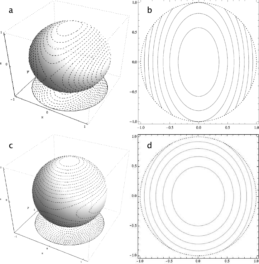
Figure 1: Intersections of the energy surfaces and the unit angular momentum sphere (a) and its projection in the $(x,y)$ plane (b) for $e_{1}=0.5$. Intersections of the energy surfaces and the unit angular momentum sphere (c) and its projection in the $(x,y)$ plane (d) for $e_{1}=0.2$.

There are four visible kinds of trajectories: closed trajectories around the two poles of the sphere $(x,y,z)=(0,0,\pm 1)$, and closed trajectories around the points $(x,y,z)=(\pm 1,0,0)$.

When the extremity of the angular momentum of the particle $\mathbf{w}$ follows a trajectory around the north pole, it means that it precesses around the angular momentum of the binary $\mathbf{k}$ with an inclination that is strictly inferior to $90^{\circ}$: in this case, the orbital motion of the particle is prograde relatively to the orbital motion of the binary.

When the extremity of the angular momentum of the particle $\mathbf{w}$ follows a trajectory around the south pole, it means that it precesses around the opposite of the angular momentum of the binary, $-\mathbf{k}$, with an inclination that is strictly superior to $90^{\circ}$: in this case, the orbital motion of the particle is retrograde relatively to the orbital motion of the binary.

When the extremity of the angular momentum of the particle $\mathbf{w}$ follows a trajectory around one of the two points $(x,y,z)=(\pm 1,0,0)$, it precesses around the direction of the perihelion of the binary or the opposite of this direction. In this case, the inclination oscillates around $\pm 90^{\circ}$.

2.4.2 Frequencies

The frequencies of these motions can be found analytically. Indeed, using equation (2.25), we see that $x$ and $y$ are on ellipses or arcs of ellipses bounded by the unit circle (figures 1.b and d show respectively the cases where $e_{1}=0.5$ and $0.2$). Thus, there is an angle $\phi$ such that:

$$x = \sqrt{\frac{1-h}{1+4e_{1}^{2}}}\cos\phi\ ,$$ (2.27)

$$y = \sqrt{\frac{1-h}{1-e_{1}^{2}}}\sin\phi\ .$$ (2.28)

Using (2.19), we can then express $z^{2}$ as:

$$z^{2}=\frac{h+4e_{1}^{2}}{1+4e_{1}^{2}}-\frac{5e_{1}^{2}}{1+4e_{1}^{2}}\frac{1-h}{1-e_{1}^{2}}\sin^{2}\phi\ .$$ (2.29)

There are two opposite values of $z$ for each $\phi$, reflecting the symmetry of the system with respect to the orbital plane of the binary. If we use expression (2.29) in combination with equation (2.18), we obtain the following equation for $\dot{\phi}$:

$$\dot{\phi} = \mp\alpha\sqrt{(1-e_{1}^{2})(h+4e_{1}^{2})}\sqrt{1-k^{2}\sin^{2}\phi}\ ,$$ (2.30)

$$\ k^{2} = \frac{5e_{1}^{2}}{1-e_{1}^{2}}\frac{1-h}{h+4e_{1}^{2}}\ .$$ (2.31)

The constant $k^{2}$ is positive because of relation (2.21). The value $k^{2}=1$ defines a limit between two dynamical regimes. If $k^{2}<1$, or equivalently if $h>e_{1}^{2}$, $\dot{\phi}$ never vanishes and the projection of $\mathbf{w}$ on the orbital plane of the binary moves along the full ellipse (2.25). In this case, $\mathbf{w}$ precesses around the angular momentum of the binary, $\mathbf{k}$. If $z>0$ the mutual inclination of the two orbits is always less than $90^{\circ}$ so the orbital motion of the particle is prograde; conversely, if $z<0$ the mutual inclination of the two orbits is always superior to $90^{\circ}$ so the orbital motion of the particle is retrograde.

If $k^{2}>1$ (or $h<e_{1}^{2}$), then $\dot{\phi}$ vanishes for $\phi_{0}=\pm\arcsin(1/k)$, changes its sign (which is accompanied by a change of sign in the $z$ variable), and the angle $\phi$ librates between $-\phi_{0}$ and $+\phi_{0}$. Thus, the projection of $\mathbf{w}$ on the orbital plane of the binary is bounded by the unit circle to stay on an arc of ellipse (2.25). In this case, $\mathbf{w}$ precesses around the direction of perihelion of the binary, so that both the inclination and the node of the particle librate around $\pm 90^{\circ}$.

In both cases, the period of the motion can be calculated with a simple quadrature using equation (2.30):

$$T=\frac{16}{3n_{1}}\frac{\mathcal{M}_{01}}{\beta_{1}}\left(\frac{a_{2}}{a_{1}}\right)^{7/2}\frac{K(k^{2})(1-e_{2}^{2})^{2}}{\sqrt{(1-e_{1}^{2})(h+4e_{1}^{2})}}\ ,\$$ (2.32)

where $K(k^{2})$ is the elliptic integral of the first kind defined by:

$$K(k^{2})=\left\{\begin{array}[]{cc}\int_{0}^{\pi/2}\frac{d\phi}{\sqrt{1-k^{2}\sin^{2}\phi}}&\text{if}\ k^{2}<1\\ \int_{0}^{\phi_{0}}\frac{d\phi}{\sqrt{1-k^{2}\sin^{2}\phi}}&\text{if}\ k^{2}>1\end{array}\right.\ .$$ (2.33)

The last case where $k^{2}=1$ (or $h=e_{1}^{2}$) corresponds to the trajectories that separate the previous two types. They link the points $(x,y,z)=(0,\pm 1,0)$, and the associated period is infinite. In the projection on the $(x,y)$ plane, these separatrices form the ellipse which is tangent to the unit circle. Since all trajectories that are inside this ellipse correspond to the precession of $\mathbf{w}$ around $\mathbf{k}$, the width $\Delta x_{\text{sep}}$ of the separating ellipse in the $(x,y)$ plane gives an indication on the proportion of such trajectories. Using equation (2.27) and the fact that $h=e_{1}^{2}$ on the separatrix, we get:

$$\Delta x_{\text{sep}}=2\sqrt{\frac{1-e_{1}^{2}}{1+4e_{1}^{2}}}$$ (2.34)

Therefore, when the inner binary is circular, this width is equal to $2$, the full width of the unit circle, and the only possible motion is precession of $\mathbf{w}$ around $\pm\mathbf{k}$. When the eccentricity of the binary increases, the width of the separatrix decreases to zero, which is a limit case since it can only be reached for a value of the binary’s eccentricity equal to 1. The precession motions of $\mathbf{w}$ around $\pm\mathbf{i}$ thus become predominant when the eccentricity of the binary grows.

2.5 Comparison with numerical studies

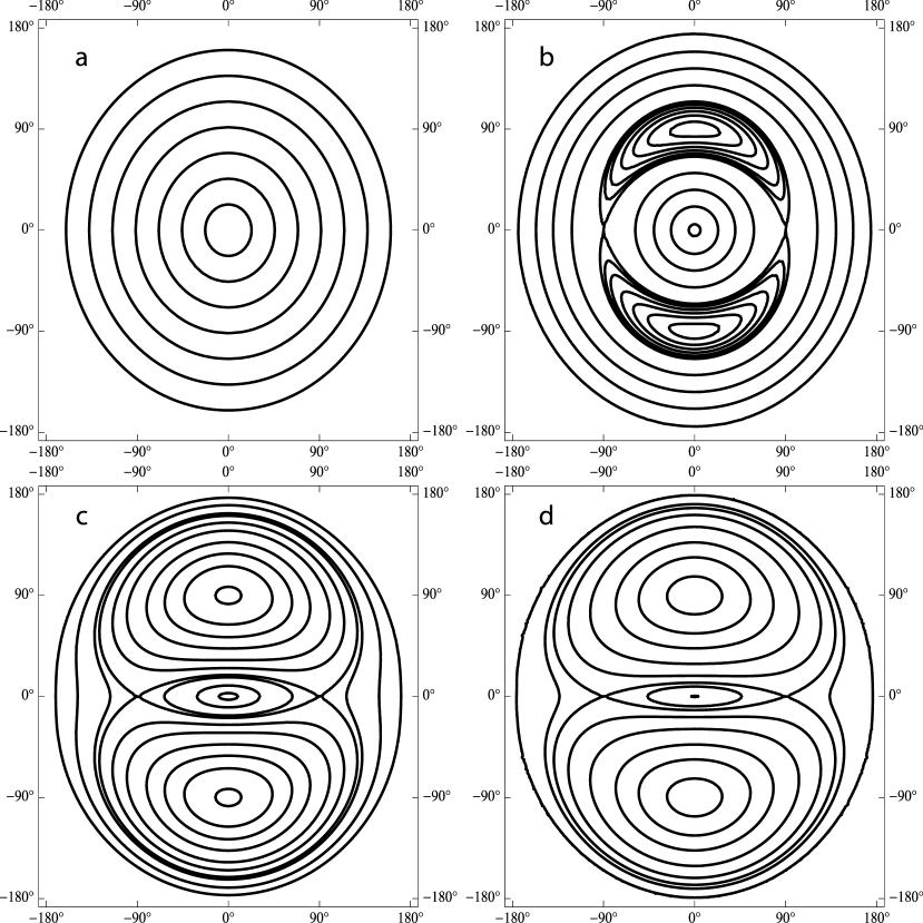
Figure 2: Energy levels of the Hamiltonian (2.8) in the $(i_{2}\cos\Omega_{2},i_{2}\sin\Omega_{2})$ plane for values of the eccentricity of the binary $e_{1}=0$ (a), $e_{1}=0.1$ (b), $e_{1}=0.79$ (c), $e_{1}=0.9$ (d).

In (Verrier & Evans, 2009), the authors investigate a family of particles at high inclinations around the binary HD 98800 Ba-Bb, which remain stable even under the perturbation of an outer third stellar companion. They isolate a nodal precession imposed by the inner binary as the stabilizing mechanism working against the destabilizing Kozai perturbations of the outer companion. They run simulations of test particles orbiting the binary HD 98800 Ba-Bb using non secular equations. They observe the libration islands around $i_{2}=\pm 90^{\circ}$ and $\Omega_{2}=\pm 90^{\circ}$ that we discussed in the previous section. As they show their results in the $(i_{2}\cos\Omega_{2},i_{2}\sin\Omega_{2})$ plane, we plotted the energy levels of the outer restricted Hamiltonian using these same coordinates for an easier comparison. Figure 2 shows these levels for different values of the eccentricity. The c. panel in particular uses the same value for the eccentricity of the binary ($e_{1}=0.79$) as figures 4 and 5 of (Verrier & Evans, 2009).

Verrier and Evans notice no apparent structure in the dynamics of the $(e_{2},\omega_{2})$ couple apart from the circulation of the perihelion. This is in agreement with the fact that the particle’s eccentricity is constant at the quadrupolar approximation.

The authors also suggest that the projection of the angular momentum of test particles along the line of apses of the binary may be an integral of motion. From the results of the previous section, it is straightforward to see that the projection $x$ of the angular momentum of test particles along the line of apses of the binary is not constant. It varies with an amplitude that decreases to $0$ when the inclination of the particle approaches $\pm 90^{\circ}$, which can be misleading when looking at numerical results for highly inclined particles. However, the norm of the angular momentum of the test particles is an integral of the secular motion.

Figure 3: Dependence of the period (2.32) with respect to the eccentricity of the binary, in normalized units. The full line corresponds to the calculated period, while the dashed line corresponds to the power-law fit given by Verrier & Evans (2009). We used a least squares method to fit the relative position of the two curves.

Finally, the authors give a power-law fit of the period of the libration of the node with respect to three parameters: the eccentricity of the binary, the ratio of the semimajor axes $a_{2}/a_{1}$, and the mass ratio of the binary, $\delta$. Their power-law is fitted using particles with fixed inclinations ($85^{\circ}$). They give in their equation (5):

$$T\propto e_{1}^{-1.1}\delta^{-0.8}\left(\frac{a_{2}}{a_{1}}\right)^{3.37}\ .$$ (2.35)

By rewriting the mass dependences of equation (2.32), we get the following analytical dependence with respect to the mass ratio and the semi-major axis of the binary:

$$T\propto\left(\frac{a_{2}}{a_{1}}\right)^{3.5}(\delta(1-\delta))^{-1}\ .$$ (2.36)

These two exponents compare very well with the fitted power law, in spite of the differences between the two models. The dependency with respect to $e_{1}$ is rather complex in equation (2.32), and it is best compared in figure 3.

The grid of initial conditions for the particles in (Verrier & Evans, 2009) extends however from 3 to 10 AU for a binary separation of 1 AU, so the quadrupolar approximation may not be sufficient to fully describe the motion of the particles with the lowest semi major axes. In particular, Verrier and Evans state that some low inclination particles show large eccentricity variations and even instability. This could be due to a low initial semi-major axis and to resonances that are eliminated in our secular model by the averaging over the mean anomalies.

3 Problem of three massive bodies

As we already stated, the quadrupolar secular three-body problem is still integrable when all the bodies have positive masses. As such, it is possible to show how the outer restricted problem we discussed in the previous section relates to the general case, and to the inner restricted case studied by Kozai (1962) and Lidov (1962). We will first express the Hamiltonian of the secular quadrupolar problem using the same vectorial method as in the previous section in order to focus on the relative movements of the orbits. In their studies of the secular quadrupolar problem, Lidov & Ziglin (1976) and Ferrer & Osacar (1994) have shown that this problem depends on two parameters. We will then point out which regions of parameter space are topologically equivalent to the outer restricted case, and which regions correspond to the inner restricted case, in order to show the continuity that exists between both situations.

3.1 Hamiltonian

Let us consider three masses $m_{0}$, $m_{1}$ and $m_{2}$, this time with $m_{2}\neq 0$. We note the barycentric coordinates and impulsions $(\mathbf{u}_{i},\mathbf{\tilde{u}}_{i})_{i=0,1,2}$. As in the previous section, we suppose that the two bodies of indices 0 and 1 form a binary and that the distance of the third body to this binary is much larger than the separation of the binary. We still note $\delta=m_{0}/(m_{0}+m_{1})$. We first perform a canonical change of variables to Jacobi coordinates,

$$\mathbf{r}_{0} =\mathbf{u}_{0} \tilde{\mathbf{r}}_{0} =\tilde{\mathbf{u}}_{0}+\tilde{\mathbf{u}}_{1}+\tilde{\mathbf{u}}_{2}=\mathbf{0}$$ (3.1)

$$\mathbf{r}_{1} =\mathbf{u}_{1}-\mathbf{u}_{0} \tilde{\mathbf{r}}_{1} =\mathbf{\tilde{u}}_{1}+(1-\delta)\tilde{\mathbf{u}}_{2}$$ (3.2)

$$\mathbf{r}_{2} =\mathbf{u}_{2}-\delta\mathbf{u}_{0}-(1-\delta)\mathbf{u}_{1} \tilde{\mathbf{r}}_{2} =\mathbf{\tilde{u}}_{2}$$ (3.3)

In these coordinates, the Hamiltonian of the three bodies is (Laskar, 1989):

$$H=\left(\frac{\tilde{\mathbf{r}}_{1}^{2}}{2\beta_{1}}-\frac{\mu_{1}\beta_{1}}{r_{1}}\right)+\frac{\tilde{\mathbf{r}}_{2}^{2}}{2\beta_{2}}\\ -Gm_{2}\left(\frac{m_{0}}{|\mathbf{r}_{2}+(1-\delta)\mathbf{r}_{1}|}+\frac{m_{1}}{|\mathbf{r}_{2}-\delta\mathbf{r}_{1}|}\right),$$ (3.4)

where $\beta_{1}^{-1}=m_{0}^{-1}+m_{1}^{-1}$, $\beta_{2}^{-1}=(m_{0}+m_{1})^{-1}+m_{2}^{-1}$, $\mu_{1}=G(m_{0}+m_{1})$ and $\mu_{2}=G(m_{0}+m_{1}+m_{2})$.

Using the fact that $r_{1}\ll r_{2}$, we expand the Hamiltonian to order two in $r_{1}/r_{2}$ as in the previous section:

$$H=\left(\frac{\tilde{\mathbf{r}}_{1}^{2}}{2\beta_{1}}-\frac{\mu_{1}\beta_{1}}{r_{1}}\right)+\left(\frac{\tilde{\mathbf{r}}_{2}^{2}}{2\beta_{2}}-\frac{\mu_{2}\beta_{2}}{r_{2}}\right)\\ -G\frac{\beta_{1}m_{2}}{2r_{2}^{3}}\left(3\frac{(\mathbf{r}_{1}.\mathbf{r}_{2})^{2}}{r_{2}^{2}}-r_{1}^{2}\right)\ .$$ (3.5)

The first two terms are Keplerian energies and are equal respectively to $-\mu_{1}\beta_{1}/2a_{1}$ and $-\mu_{2}\beta_{2}/2a_{2}$, where $a_{1}$ and $a_{2}$ are the semi major axes of the inner and the outer body in our system of coordinates.

We now average over the two mean anomalies $M_{1}$ and $M_{2}$ in order to get the secular part of the Hamiltonian. We will define 4 unit vectors which are analogous to the 4 vectors we used in the first section: $(\mathbf{i}_{1},\mathbf{j}_{1},\mathbf{k}_{1})$ are tied to the orbit of the inner binary; $\mathbf{i}_{1}$ points in the direction of the perihelion of the inner binary, $\mathbf{k}_{1}$ points in the direction of its angular momentum, and $\mathbf{j}_{1}=\mathbf{k}_{1}\wedge\mathbf{i}_{1}$. The last vector $\mathbf{k}_{2}$ is colinear to the angular momentum of the outer body. In this section, the vectors tied to the orbit of the inner binary will no longer have fixed directions.

Using the same averaging formulae as in the previous section and using the fact that $(\mathbf{i}_{1}.\mathbf{k}_{2})^{2}+(\mathbf{j}_{1}.\mathbf{k}_{2})^{2}+(\mathbf{k}_{1}.\mathbf{k}_{2})^{2}=\mathbf{k}_{2}^{2}=1$, we can write:

$$\left\langle H\right\rangle_{M_{1},M_{2}}=-\frac{\mu_{1}\beta_{1}}{2a_{1}}-\frac{\mu_{2}\beta_{2}}{2a_{2}}-\frac{3}{8}\frac{Gm_{2}\beta_{1}}{(1-e_{2}^{2})^{3/2}}\frac{a_{1}^{2}}{a_{2}^{3}}\\ \times\left[-\frac{1}{3}+2e_{1}^{2}+(1-e_{1}^{2})\mathopen{(}\mathbf{k}_{1}.\mathbf{k}_{2}\mathclose{)}^{2}-5e_{1}^{2}\mathopen{(}\mathbf{i}_{1}.\mathbf{k}_{2}\mathclose{)}^{2}\right]\ .$$ (3.6)

After averaging over the two mean anomalies, the semi-major axes are constant. There are thus four degrees of freedom in the system, associated to the two eccentricities and the two inclinations. As we explained in the previous section, the argument of perihelion of the outer body does not appear in the quadrupolar expansion, and thus the norm of the angular momentum of the outer body $G_{2}=\beta_{2}\sqrt{\mu_{2}a_{2}(1-e_{2}^{2})}$, is constant. This implies that its eccentricity $e_{2}$ is constant. Using the reduction of the nodes would leave only one degree of freedom in the reduced Hamiltonian, associated to the couple $(e_{1},\omega_{1})$. The full reduction of the Hamiltonian and its expression in elliptical variables is the approach that has been used widely, since it yields a very similar Hamiltonian function as in the inner restricted problem (Harrington, 1969; Lidov & Ziglin, 1976; Ferrer & Osacar, 1994).

We want however to look at the motion of the nodes, or equivalently the motion of the vector $\mathbf{k}_{2}$ in the moving frame $(\mathbf{i}_{1},\mathbf{j}_{1},\mathbf{k}_{1})$ of the orbit of the second body.

In order to easily compute the equations of motion, we introduce two vectors associated to the orbit of the binary that are colinear to $\mathbf{i}_{1}$ and $\mathbf{k}_{1}$, and include in their norm the eccentricity of the binary, as in (Tremaine et al., 2009):

$$\mathcal{K}_{1} =\sqrt{1-e_{1}^{2}}\mathbf{k}_{1}\ , \mathcal{I}_{1} =e_{1}\mathbf{i}_{1}\ .$$ (3.7)

If we drop all the constant terms in equation 3.6 and use the above vectors, we get:

$$\left\langle H\right\rangle_{M_{1},M_{2}}=-\frac{\alpha^{\prime}G_{2}}{2}\left[2\mathcal{I}_{1}^{2}+(\mathcal{K}_{1}.\mathbf{k}_{2})^{2}-5(\mathcal{I}_{1}.\mathbf{k}_{2})^{2}\right]\ ,$$ (3.8)

where

$$\alpha^{\prime}=\frac{3}{4}n_{1}\left(\frac{a_{1}}{a_{2}}\right)^{7/2}\frac{\beta_{1}}{\mathcal{M}_{01}}\frac{1}{(1-e_{2}^{2})^{2}}\sqrt{1+\frac{m_{2}}{\mathcal{M}_{01}}}\ ,$$ (3.9)

and $\mathcal{M}_{01},n_{1}$ are defined as in section 2.

3.2 Equations of motion

The components of $\mathcal{K}_{1},\mathcal{I}_{1}$ and $\mathbf{k}_{2}$ have the following Poisson brackets (Borisov & Mamaev, 2005; Boué & Laskar, 2006):

$$\{\mathcal{K}_{1i},\mathcal{K}_{1j}\} =-\frac{\epsilon_{ijk}}{\Lambda_{1}}\mathcal{K}_{1k}\,, \{k_{2i},k_{2j}\} =-\frac{\epsilon_{ijk}}{G_{2}}k_{2k}\,,$$ (3.10)

$$\{\mathcal{I}_{1i},\mathcal{I}_{1j}\} =-\frac{\epsilon_{ijk}}{\Lambda_{1}}\mathcal{K}_{1k}\,, \{\mathcal{K}_{1i},\mathcal{I}_{1j}\} =-\frac{\epsilon_{ijk}}{\Lambda_{1}}\mathcal{I}_{1k}\,,$$ (3.11)

where $\Lambda_{1}=\beta_{1}\sqrt{\mu_{1}a_{1}}$ and $\epsilon_{ijk}$ is the Levi-Civita symbol.

The equations of motion for the three vectors are thus:

$$\dot{\mathcal{K}}_{1} = -\frac{1}{\Lambda_{1}}\left(\mathcal{K}_{1}\wedge\nabla_{\mathcal{K}_{1}}H+\mathcal{I}_{1}\wedge\nabla_{\mathcal{I}_{1}}H\right)\ ,$$ (3.12)

$$\dot{\mathcal{I}}_{1} = -\frac{1}{\Lambda_{1}}\left(\mathcal{I}_{1}\wedge\nabla_{\mathcal{K}_{1}}H+\mathcal{K}_{1}\wedge\nabla_{\mathcal{I}_{1}}H\right)\ ,$$ (3.13)

$$\dot{\mathbf{k}}_{2} = -\frac{1}{G_{2}}\mathbf{k}_{2}\wedge\nabla_{\mathbf{k}_{2}}H\ .$$ (3.14)

In order to look at the motion of the vector $\mathbf{k}_{2}$ in the moving frame $(\mathbf{i}_{1},\mathbf{j}_{1},\mathbf{k}_{1})$ of the orbit of the second body, we use as Boué & Laskar (2006) the above system to derive equations for $x=(\mathbf{k}_{2}.\mathbf{i}_{1})$, $y=(\mathbf{k}_{2}.\mathbf{j}_{1})$, $z=(\mathbf{k}_{2}.\mathbf{k}_{1})$ and $e_{1}$. Indeed, $x=(\mathbf{k}_{2}.\mathcal{I}_{1})/|\mathcal{I}_{1}|$, $z=(\mathbf{k}_{2}.\mathcal{K}_{1})/|\mathcal{K}_{1}|$, $e_{1}=|\mathcal{I}_{1}|$, and $y$ is obtained using the identity $x^{2}+y^{2}+z^{2}=1$:

$$\dot{x} =\alpha^{\prime}(1-e_{1}^{2})yz+\alpha^{\prime}\frac{G_{2}}{\Lambda_{1}}\sqrt{1-e_{1}^{2}}y(2-5x^{2})$$ (3.15)

$$\dot{y} =-\alpha^{\prime}(1+4e_{1}^{2})xz$$

$$\phantom{=\dots}-\alpha^{\prime}\frac{G_{2}}{\Lambda_{1}}\frac{x}{\sqrt{1-e_{1}^{2}}}[(1-e_{1}^{2})(2-5x^{2})+5e_{1}^{2}z^{2}]$$ (3.16)

$$\dot{z} =5\alpha^{\prime}e_{1}^{2}xy+\alpha^{\prime}\frac{G_{2}}{\Lambda_{1}}\frac{5e_{1}^{2}}{\sqrt{1-e_{1}^{2}}}xyz$$ (3.17)

$$\dot{e}_{1} =\alpha^{\prime}\frac{G_{2}}{\Lambda_{1}}5e_{1}\sqrt{1-e_{1}^{2}}xy$$ (3.18)

The equations for $x,y$ and $z$ contain two terms: the first one is identical to the outer restricted system, and the second one includes the motion of the reference frame $(\mathbf{i}_{1},\mathbf{j}_{1},\mathbf{k}_{1})$ induced by the interaction with the third body. Note that when $\Lambda_{1}$ is very large compared to $G_{2}$ so that we can assume that $G_{2}/\Lambda_{1}$ is equal to zero, which corresponds to the case where $m_{2}\ll m_{0}\text{ and }m_{1}$, the above system is identical to the outer restricted system (2.16)–(2.18).

The conservation of the total angular momentum $\mathbf{C}=\mathbf{G}_{1}+\mathbf{G}_{2}$ introduces the two main parameters of the problem. Indeed,

$$\Lambda_{1}^{2}(1-e_{1}^{2})+G_{2}^{2}+2\Lambda_{1}\sqrt{1-e_{1}^{2}}G_{2}z=C^{2}\ .$$ (3.19)

We note $\gamma=C/\Lambda_{1}$, $\gamma_{2}=G_{2}/\Lambda_{1}$. The above expression of the norm of the total angular momentum can be rewritten as a second degree equation giving $\sqrt{1-e_{1}^{2}}$ as a function of $z$ using the two parameters $\gamma$ and $\gamma_{2}$:

$$(1-e_{1})^{2}+2\gamma_{2}z\sqrt{1-e_{1}^{2}}+\gamma_{2}^{2}-\gamma^{2}=0\ .$$ (3.20)

The Hamiltonian can then be rewritten as:

$$\left\langle H\right\rangle=-\frac{1}{2}\alpha^{\prime}\Lambda_{1}\gamma_{2}[z^{2}+e_{1}^{2}(2-z^{2}-5x^{2})]\ .$$ (3.21)

The inequalities $-1\leqslant z\leqslant 1$ and $0\leqslant e_{1}<1$ give the boundaries of the parameter space and the range of possible values of $e_{1}$ for any given couple of parameters $(\gamma,\gamma_{2})$:

$$|\gamma-\gamma_{2}| \leqslant 1\ ,$$ (3.22)

$$|\gamma-\gamma_{2}| \leqslant\sqrt{1-e_{1}^{2}}\leqslant\min[\gamma+\gamma_{2},1]\ .$$ (3.23)

With these notations, the outer restricted problem of section 2 corresponds to the limit where $\gamma_{2}=0$, and in this case $e_{1}=\sqrt{1-\gamma^{2}}$ is constant as we saw. Note that when $\gamma_{2}>\gamma$, we have $G_{2}>C$, so this part of the parameter space contains only retrograde motions. Our aim in this paper is to show the continuity between the outer restricted case we studied in section 2, and the inner restricted case that was investigated by Kozai (1962) and Lidov (1962). Both these problems lie in the region of parameter space where $\gamma>\gamma_{2}$ so we will restrict our study to this case.

In our case where $\gamma>\gamma_{2}$, there is only one acceptable root to equation (3.20), which is:

$$\sqrt{1-e^{2}_{1}}=-\gamma_{2}z+\sqrt{(\gamma_{2}z)^{2}+\gamma^{2}-\gamma_{2}^{2}}\ .$$ (3.24)

This relation implies that $e_{1}$ is a growing function of $z$. Note that $z=\cos i_{2}$, where $i_{2}$ is the inclination of the outer body in the reference frame of the inner binary. As such, coplanar prograde motions ($z=1$) will always occur for the maximal value of the eccentricity of the inner binary:

$$e_{1,\max}=\sqrt{1-(\gamma-\gamma_{2})^{2}}\ .$$ (3.25)

Conversely, low eccentricities for the binary will be associated to lower values of $z$, and thus higher inclinations. Relation (3.23) implies that the inner binary can only have a circular motion if $\gamma+\gamma_{2}\geqslant 1$. In this case, coplanar retrograde motion ($z=-1$) is not allowed, and the lowest value of $z$ is:

$$z_{0}=\cos i_{2,\max}=\frac{\gamma^{2}-\gamma_{2}^{2}-1}{2\gamma_{2}}\ .$$ (3.26)

When $\gamma+\gamma_{2}<1$ however, coplanar retrograde motion ($z=-1$) is possible and the associated value of the eccentricity of the binary is:

$$e_{1,\min}=\sqrt{1-(\gamma+\gamma_{2})^{2}}\ .$$ (3.27)

Figure 4: Parameter Space. The dark gray areas are excluded by equation (3.22), the light gray area correspond to the part of parameter space corresponding to $\gamma_{2}\geqslant\gamma$ which we do not study. The dotted line $\gamma+\gamma_{2}=1$ separates the zone where there can be coplanar retrograde motion associated to a minimum eccentricity for the inner binary that is strictly higher than $0$ (below the dotted line) and the zone where the inner binary can be circular but the inclination is bounded (see section A.2). In zone O, the problem is topologically equivalent to the outer restricted problem. In zones I and I’ it is topologically equivalent to the inner restricted problem, with zone I being equivalent to situations above the critical inclination and zone I’ being equivalent to situations under the critical inclination. The letters a–f correspond to the values of the parameters used to plot the corresponding panels in figures 5 and 6.

3.3 Dynamical regimes

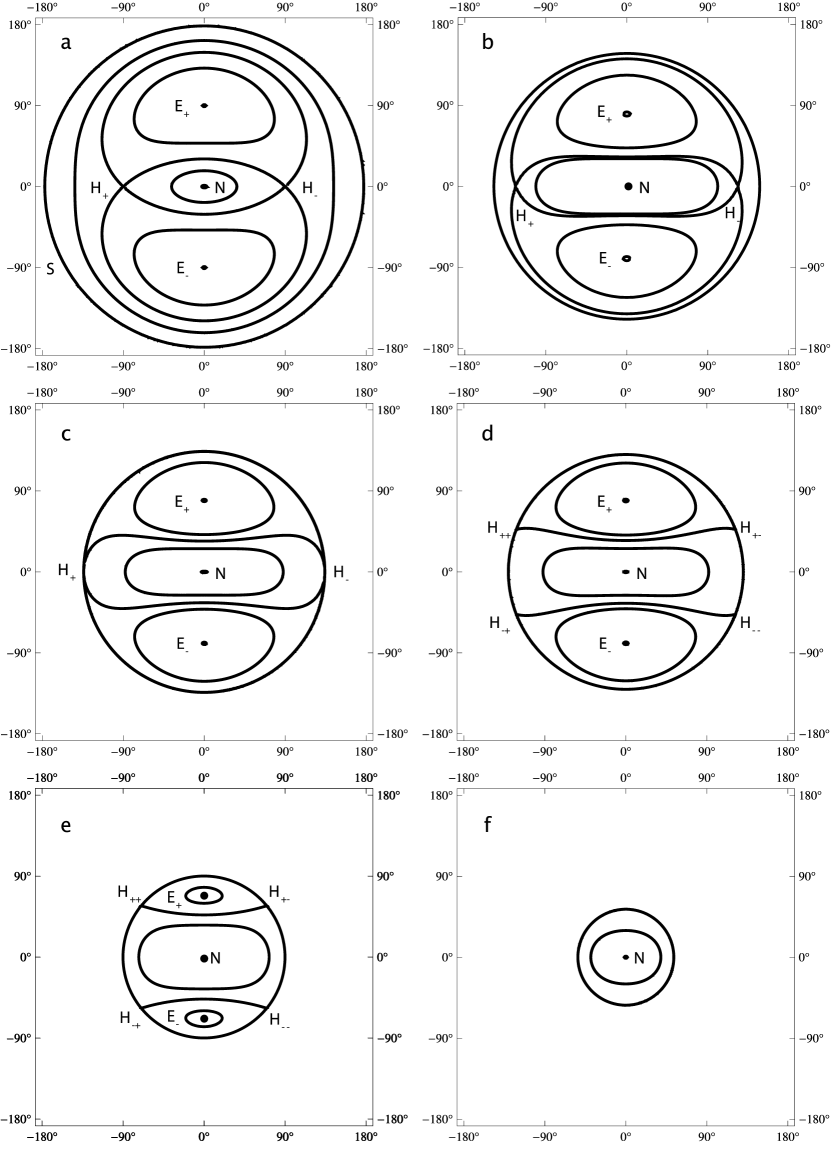
Figure 5: Trajectories in the $(i_{2}\cos\Omega_{2},i_{2}\sin\Omega_{2})$ plane for different values of the parameters. See section 3.3 for a detailed discussion and appendix A for calculations. a: $(\gamma,\gamma_{2})=(0.8,0)$ outer restricted case with $e_{1}=0.6$; b: $(\gamma,\gamma_{2})=(0.8,0.25)$; c: $\gamma=0.8,\,\gamma_{2}^{2}=(1/3)(1-\gamma^{2})$; d: $(\gamma,\gamma_{2})=(0.8,0.4)$; e: $(\gamma,\gamma_{2})=(1.08,0.4)$; f: $(\gamma,\gamma_{2})=(1.28,0.4)$.

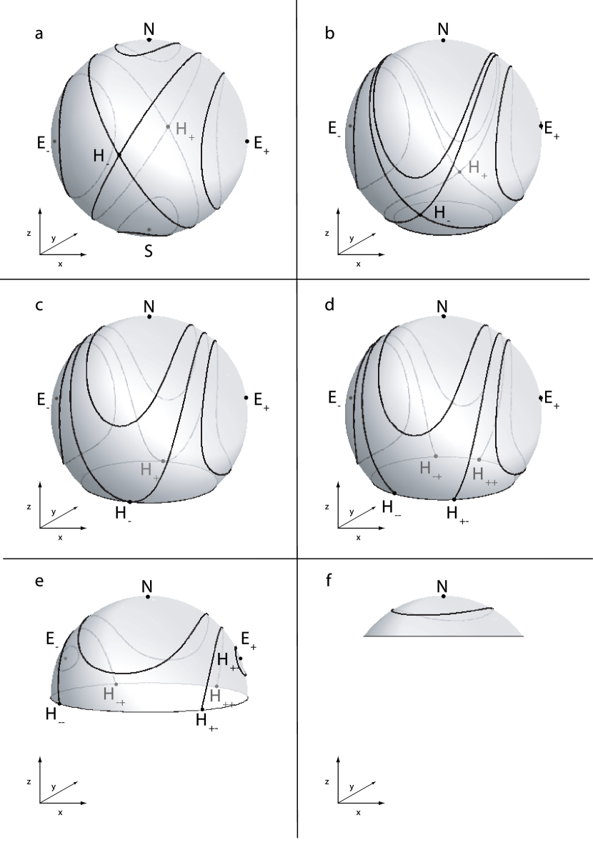
Figure 6: Trajectories on the unit angular momentum sphere for different values of the parameters. See section 3.3 for a detailed discussion and appendix A for calculations. a: $(\gamma,\gamma_{2})=(0.8,0)$ outer restricted case with $e_{1}=0.6$; b: $(\gamma,\gamma_{2})=(0.8,0.25)$; c: $\gamma=0.8,\,\gamma_{2}^{2}=(1/3)(1-\gamma^{2})$; d: $(\gamma,\gamma_{2})=(0.8,0.4)$; e: $(\gamma,\gamma_{2})=(1.08,0.4)$; f: $(\gamma,\gamma_{2})=(1.28,0.4)$.

In appendix A, we briefly derive in the framework of the present study the fixed points of the system and the boundaries of the dynamical regimes in parameter space that are given in (Ferrer & Osacar, 1994). The fixed points are named as follow: the north pole is called $N$, and the south pole $S$; linearly stable fixed points are named $E$, as elliptic, and linearly unstable points are named $H$, as hyperbolic; finally, signs are placed as indices to refer to the symmetry of the problem with respect to the two planes $x=0$ and $y=0$. There are three dynamical regimes in the region of parameter space we study.

In region O of figure 4, the parameter $\gamma_{2}=G_{2}/\Lambda_{1}$ is small (less than 1/2). This is the case in particular when the mass ratio $m_{2}/m_{1}$ is small. Moreover, $\gamma^{2}+3\gamma_{2}^{2}<1$. The phase space is topologically equivalent to the outer restricted problem of section 2. The north pole, which corresponds to coplanar prograde motion with maximal eccentricity for the binary is linearly stable. There are two additional stable fixed points $\text{E}_{\pm}$ in the plane $y=0$ (see section A.4). They belong to the same family as the fixed points $y=z=0$, $x=\pm 1$ of the outer restricted problem that are responsible for the stable high inclination orbits observed by Verrier & Evans (2009). When $\gamma+\gamma_{2}\leqslant 1$, the south pole which corresponds to coplanar retrograde motion with minimal eccentricity for the binary, is also linearly stable. The a panels of figures 5 and 6 provide a visualisation of the topology of this case. When $\gamma+\gamma_{2}>1$, the south pole is no longer accessible as stated in the previous section. It is however replaced by a stable trajectory at a maximal inclination given by equation (3.26), as can be seen on panel b of figures 5 and 6. This trajectory corresponds to a circular inner binary (see section A.2). Finally, there are two unstable points $\text{H}_{\pm}$ in the $x=0$ plane that belong to the same family as the unstable points of the outer restricted problem $x=z=0$, $y=\pm 1$ (see section A.3).

Panels c of figures 5 and 6 show the limiting case between regions O and I. On this boundary, $\gamma^{2}+3\gamma_{2}^{2}=1$. The two unstable points $H_{\pm}$ are now located on the boundary of the accessible part of the sphere.

Regions I and I’ of figure 4 are both in the part of the parameter space defined by $\gamma^{2}+3\gamma_{2}^{2}>1$. In this zone, the problem becomes topologically equivalent to the inner restricted problem studied by Lidov (1962) and Kozai (1962). In the inner restricted case, there is a critical value of the inclination ($\cos i_{2}=\sqrt{3/5}$) under which a circular inner binary is always linearly stable, and above which a circular inner binary is always linearly unstable, giving rise to Kozai cycles.

In region I of figure 4, the dynamical regime is topologically equivalent to the inner restricted problem in the case where the inclination is superior to the critical value. The limit trajectory $z=z_{0}$ which corresponds to a circular inner binary becomes linearly unstable. However, the north pole and the two fixed points $\text{E}_{\pm}$ are still stable. In the inner restricted phase space, when the inclination is superior to the critical value, there are two possible behaviours for the periastron of the inner particle: it can either circulate, or librate around $\pm 90^{\circ}$. In our representation, the circulation case corresponds to trajectories around the north pole, and the libration islands correspond to the two fixed points $\text{E}_{\pm}$. This is shown in panels d and e in figures 5 and 6.

In region I’ of figure 4, the dynamical regime is topologically equivalent to the inner restricted problem in the case where the inclination is inferior to the critical value. Only one stable fixed point remains, on the north pole of the sphere, associated to prograde coplanar motion. This is shown in panel f in figures 5 and 6.

In both regions I and I’, the parameter $\gamma_{2}=G_{2}/\Lambda_{1}$ can take higher values. This is in particular true when the mass ratio $m_{2}/m_{1}$ increases.

The curve between regions I and I’ is linked to the critical inclination that is defined in the inner restricted case. Indeed, along that curve, given by equation A.10, we have the following limits when $\gamma\rightarrow\infty$:

$$\frac{\gamma_{2}}{\gamma} \rightarrow 1\,, \gamma_{2}-\gamma\rightarrow-\sqrt{\frac{3}{5}}\ .$$ (3.28)

When $G_{2}$ is very large compared to $G_{1}$, we can make the following first order expansion:

$$\gamma_{2}-\gamma =\frac{G_{2}-C}{\Lambda_{1}}$$ (3.29)

$$=\frac{G_{2}-\sqrt{G_{2}^{2}+G_{1}^{2}+2(\mathbf{G}_{2}.\mathbf{G}_{1})}}{\Lambda_{1}}$$ (3.30)

$$\approx\frac{G_{2}-G_{2}(1+(\mathbf{G}_{2}.\mathbf{G}_{1})/G_{2}^{2})}{\Lambda_{1}}$$ (3.31)

$$\approx-\frac{(\mathbf{G}_{2}.\mathbf{G}_{1})}{\Lambda_{1}G_{2}}$$ (3.32)

$$\approx-z\sqrt{1-e_{1}^{2}}\ .$$ (3.33)

As such, we see that along the border between regions I and I’, when $\gamma$ and $\gamma_{2}$ both tend to infinity, we have the relation

$$z\sqrt{1-e_{1}^{2}}\approx\sqrt{\frac{3}{5}}\ .$$ (3.34)

Recall that $z=\cos i_{2}$, where $i_{2}$ is the inclination of the outer orbit in the reference frame of the inner orbit. Thus, the inclination of the inner orbit relatively to the outer orbit is $i_{1}=-i_{2}$, and the above equation becomes:

$$\cos i_{1}\sqrt{1-e_{1}^{2}}\approx\sqrt{\frac{3}{5}}\ .$$ (3.35)

This relation is precisely the one giving the critical value of the normal component of the angular momentum of the inner body in the inner restricted problem.

Conclusion

We first studied the case of a massless particle orbiting a binary at a long distance, and, in the secular and quadrupolar approximations, gave a full analytical description of the motion along with the expression of the period of the secular motion. When the inner binary is circular, only nodal precession takes place. However, when the binary is elliptic, libration islands appear at high inclinations, and these islands grow bigger when the eccentricity of the binary rises. Verrier & Evans (2008, 2009) observe a similar nodal libration in their study of the stability of particle populations in the quadruple stellar system HD 98800, and we showed that the analytical framework that we derived for the outer restricted problem is well suited to explain the results of Verrier and Evans.

The quadrupolar secular three-body problem is still integrable when all the bodies have positive masses (Harrington, 1969; Lidov & Ziglin, 1976; Ferrer & Osacar, 1994). Using a vectorial formalism as (Boué & Laskar, 2006, 2009; Tremaine et al., 2009), we looked at this problem from the point of view of the outer restricted case. We showed how the outer restricted problem relates to the general case, and to the inner restricted case studied by Kozai (1962) and Lidov (1962): when the mass of the outer body is small enough compared to the mass of the inner body, the general case behaves similarly to the outer restricted problem. When the mass of the outer body increases enough, the general case behaves like the inner restricted problem. We gave an expression of the boundary between these two regimes.

The outer restricted problem and its generalization to the non restricted case provide an interesting starting point in the study of circumbinary planetary systems, such as the one discovered recently around the eclipsing sdB+M system HW Virginis (Lee et al., 2009). In this system, the inner binary is very tight with a period of 2.8 hr, while the proposed planetary companions have periods of 9.1 yr and 15.8 yr, so the quadrupolar expansion is fully justified. Another field of application of the outer restricted problem is the study of the motion of stars orbiting around binary black holes (Mikkola & Merritt, 2008; Gillessen et al., 2009; Merritt et al., 2009).

Appendix A Fixed points and bifurcations

The fixed points and boundaries presented in section 3.3 have already been studied by Lidov & Ziglin (1976) and Ferrer & Osacar (1994). We briefly present here their derivation in the framework of the present formalism. With the notations of section 3, we will limit ourselves to $\gamma>\gamma_{2}$.

A.1 Poles of the sphere, $x=y=0$

This case corresponds to case 1 in section 5 of (Ferrer & Osacar, 1994). Note that their sphere is constructed using the eccentricity and perihelion of the inner binary, and is thus different from our angular momentum sphere.

For all values of the parameters in the domain we study, the north pole $z=1$, which corresponds to coplanar prograde motion, is a fixed point of the system. The associated eccentricity of the inner binary is:

$$e_{1,\max}=\sqrt{1-(\gamma-\gamma_{2})^{2}}\ .$$ (A.1)

It is the maximal value of the eccentricity. This fixed point is always linearly stable. It is noted N in figures 5 and 6. Figure 5 shows the lines of equal energy in the $(i_{2}\cos\Omega_{2},i_{2}\sin\Omega_{2})$ plane, and figure 6 shows these lines plotted on the sphere of unit angular momentum of the outer body $\mathbf{k}_{2}^{2}=1$.

When $\gamma+\gamma_{2}<1$ (under the dotted line in figure 4), the south pole $z=-1$ (noted S in the following figures), which corresponds to coplanar retrograde motion, is also a linearly stable fixed point of the system. The eccentricity of the inner binary is minimal and equal to:

$$e_{1,\min}=\sqrt{1-(\gamma+\gamma_{2})^{2}}\ .$$ (A.2)

Note that in this region of parameter space, the inner binary cannot be circular.

When $\gamma+\gamma_{2}\geqslant 1$ (above the dotted line in figure 4), the minimal eccentricity of the binary is $0$ as deduced from (3.23). The south pole $z=-1$ does not correspond to a real value of the eccentricity in this case. This limit however is not a bifurcation strictly speaking. When crossing it, the stable south pole of the sphere is replaced by a stable trajectory at maximal inclination.

A.2 Circular Trajectories for the inner binary

In the region of parameter space where circular trajectories exist for the binary (above the dotted line in figure 4), the value of $z$ which corresponds to such trajectories is minimal and equal to:

$$z_{0}=\frac{\gamma^{2}-\gamma_{2}^{2}-1}{2\gamma_{2}}\ .$$ (A.3)

The equations of motion on the small circle of the sphere $z=z_{0}$ are:

$$\dot{x}_{\phantom{1}} = \phantom{-}\alpha^{\prime}y(z_{0}+\gamma_{2}(2-5x^{2}))\ ,$$ (A.4)

$$\dot{y}_{\phantom{1}} = -\alpha^{\prime}x(z_{0}+\gamma_{2}(2-5x^{2}))\ ,$$ (A.5)

$$\dot{z}_{\phantom{1}} = \phantom{-}0\ ,$$ (A.6)

$$\dot{e}_{1} = \phantom{-}0\ .$$ (A.7)

The right hand sides of equations (A.4) and (A.5) vanish for a certain value of $x$ equal to:

$$x_{0}^{2}=\frac{\gamma^{2}+3\gamma_{2}^{2}-1}{10\gamma_{2}^{2}}\ .$$ (A.8)

The curve $\gamma^{2}+3\gamma_{2}^{2}=1$ separates in figure 4 the regions noted O and I. We can distinguish three cases:

1. $\gamma^{2}+3\gamma_{2}^{2}<1$. In region O of figure 4, $x_{0}^{2}<0$ so there is no fixed point on the circle $z=z_{0}$. As such, this circle is a trajectory for which the inner binary is circular and the outer orbit precesses at a fixed inclination given by $i_{2,\max}=\text{ArcCos}\,z_{0}$. Moreover, this trajectory is linearly stable.

2. $\gamma^{2}+3\gamma_{2}^{2}=1$. There are two fixed points on the circle $z=z_{0}$ at the coordinates $(x=0,y=\pm\sqrt{1-z_{0}^{2}})$.

3. $\gamma^{2}+3\gamma_{2}^{2}>1$. In this case, we must also check that $y_{0}^{2}=1-x_{0}^{2}-z_{0}^{2}\geqslant 0$. The limit case where there is equality yields:

   $$5\gamma_{2}^{4}-(4+10\gamma^{2})\gamma_{2}^{2}+(5\gamma^{4}-8\gamma^{2}+3)=0\ .$$ (A.9)

This boundary limits the regions I and I’ in figure 4. When solving the above equation for $\gamma_{2}^{2}$ and selecting only the relevant solution satisfying $\gamma>\gamma_{2}\,,\gamma+\gamma_{2}\geqslant 1$, we obtain a solution that corresponds to equation 44 in section 5.2 of (Ferrer & Osacar, 1994) and that can be written using our notations as:

$$\gamma_{2}^{2}=\frac{2+5\gamma^{2}-\sqrt{60\gamma^{2}-11}}{5}\,,\quad\gamma+\gamma_{2}\geqslant 1\ .$$ (A.10)

In region I, $y_{0}^{2}>0$ so there are four fixed points on the circle $z=z_{0}$, at the coordinates $(\pm x_{0},\pm y_{0})$. They are noted $\text{H}_{\pm\pm}$, in panels d and e of figures 5 and 6. Moreover, the trajectories that correspond to circular binaries are unstable in this zone. In region I’ however, $y_{0}^{2}<0$ so we are again in a region of parameter space where there are no fixed points on the circle $z=z_{0}$, and the trajectories associated to circular binaries are again stable.

A.3 The $x=0$ plane

When $x=0$, the only non trivial equation remaining in system (3.15)–(3.18) is $\dot{x}=0$. Looking for a fixed point different from $x=y=0$, we have to solve

$$z\sqrt{1-e_{1}^{2}}+2\gamma_{2}=0\ ,$$ (A.11)

which after using relation (3.20) yields:

$$e_{1} = \sqrt{1-\gamma^{2}-3\gamma_{2}^{2}}\ ,$$ (A.12)

$$x = 0\ ,$$ (A.13)

$$y = \pm\frac{\sqrt{\gamma^{2}-\gamma_{2}^{2}}}{\sqrt{\gamma^{2}+3\gamma_{2}^{2}}}\ ,$$ (A.14)

$$z = -\frac{2\gamma_{2}}{\sqrt{\gamma^{2}+3\gamma_{2}^{2}}}\ .$$ (A.15)

We thus have two symmetric fixed points in the plane $x=0$. They are noted $\text{H}_{\pm}$ in figures 5 and 6. For these fixed points to exist, the associated eccentricity must be a real number. As such, their domain of existence is the region noted O in figure 4. This is case 2.1 in section 5 of (Ferrer & Osacar, 1994).

These two fixed points are linearly unstable in their domain of existence. Note that in the outer restricted problem ($\gamma_{2}=0$), these fixed points are simply $x=z=0,y=\pm 1$.

A.4 The $y=0$ plane

When $y=0$, the only non trivial equation we must solve is $\dot{y}=0$. Here again, we look for another fixed point than $x=y=0$, thus we have to solve:

$$(1+4e_{1}^{2})z+\frac{\gamma_{2}}{\sqrt{1-e_{1}^{2}}}[(1-e_{1}^{2})(2-5x^{2})+5e_{1}^{2}z^{2}]=0\ .$$ (A.16)

Substituting $1-z^{2}$ in place of $x^{2}$ and then $\sqrt{1-e_{1}^{2}}$ in place of $z$ using (3.20), we get:

$$(1-e_{1}^{2})^{3}-\left(\gamma^{2}+\frac{1}{2}\gamma_{2}^{2}+\frac{5}{8}\right)(1-e_{1}^{2})^{2}+\frac{5}{8}(\gamma^{2}-\gamma_{2}^{2})^{2}=0$$ (A.17)

This equation is the same as equation number 40 in (Ferrer & Osacar, 1994). In our region of parameter space, there is at most one root which satisfies to the constraint (3.23). The curve separating the zone where there is one solution and the zone where there is no solution corresponds to the case where the limit value $e_{1}=0$ is a solution, and coincides with the boundary between regions I and I’ in figure 4 which is given by equation (A.10).

When there is a solution, the value of $e_{1}$ can be translated into a value of $z$ using (3.20). Since $y=0$, we get two values of $x=\pm\sqrt{1-z^{2}}$, and there are thus two symmetric fixed points on the sphere, which are both linearly stable. They are noted $\text{E}_{\pm}$ in figures 5 and 6. When $\gamma_{2}=0$, these fixed points become simply $y=z=0$, $x=\pm 1$, which are responsible of the stable orbits at high inclination as discussed in the previous sections.

References

- Borisov & Mamaev (2005) Borisov A. V., Mamaev I. S., 2005, Dynamics of the Rigid Body (in Russian). R&C Dynamics, Moscow, (http://ics.org.ru/)
- Boué & Laskar (2006) Boué G., Laskar J., 2006, Icarus, 185, 312
- Boué & Laskar (2009) Boué G., Laskar J., 2009, Icarus, 201, 750
- Ferrer & Osacar (1994) Ferrer S., Osacar C., 1994, Celest. Mech. Dyn. Astron., 58, 245
- Gillessen et al. (2009) Gillessen S., Eisenhauer F., Trippe S., Alexander T., Genzel R., Martins F., Ott T., 2009, ApJ, 692, 1075
- Harrington (1969) Harrington R. S., 1969, Celest. Mech., 1, 200
- Kinoshita & Nakai (2007) Kinoshita H., Nakai H., 2007, Celest. Mech. Dyn. Astron., 98, 67
- Kozai (1962) Kozai Y., 1962, AJ, 67, 591
- Laskar (1989) Laskar J., 1989, in Benest D., Froeschle C., eds, Modern Methods in Celestial Mechanics, Systèmes de Variables et Eléments. Editions Frontières, pp 63–87
- Lee et al. (2009) Lee J. W., Kim S.-L., Kim C.-H., Koch R. H., Lee C.-U., Kim H.-I., Park J.-H., 2009, AJ, 137, 3181
- Lidov (1962) Lidov M. L., 1962, P&SS, 9, 719
- Lidov & Ziglin (1976) Lidov M. L., Ziglin S. L., 1976, Celest. Mech., 13, 471
- Malige et al. (2002) Malige F., Robutel P., Laskar J., 2002, Celest. Mech. Dyn. Astron., 84, 283
- Merritt et al. (2009) Merritt D., Gualandris A., Mikkola S., 2009, ApJ Lett., 693, L35
- Mikkola & Merritt (2008) Mikkola S., Merritt D., 2008, AJ, 135, 2398
- Palacián & Yanguas (2006) Palacián J. F., Yanguas P., 2006, Celest. Mech. Dyn. Astron., 95, 81
- Palacián et al. (2006) Palacián J. F., Yanguas P., Fernández S., Nicotra M. A., 2006, Physica D Nonlinear Phenomena, 213, 15
- Poincaré (1905) Poincaré H., 1905, Leçons de mécanique céleste professées à la Sorbonne
- Touma et al. (2009) Touma J. R., Tremaine S., Kazandjian M. V., 2009, MNRAS, 394, 1085
- Tremaine et al. (2009) Tremaine S., Touma J., Namouni F., 2009, AJ, 137, 3706
- Verrier & Evans (2008) Verrier P. E., Evans N. W., 2008, MNRAS, 390, 1377
- Verrier & Evans (2009) Verrier P. E., Evans N. W., 2009, MNRAS, 394, 1721