Cosmological implications of massive gravitons

Abstract

The van Dam-Veltman-Zakharov (vDVZ) discontinuity requires that the mass $m$ of the graviton is exactly zero, otherwise measurements of the deflection of starlight by the Sun and the precession of Mercury’s perihelion would conflict with their theoretical values. This theoretical discontinuity is open to question for numerous reasons. In this paper we show from a phenomenological viewpoint that the $m>0$ hypothesis is in accord with Supernova Ia and CMB observations, and that the large scale structure of the universe suggests that $m\sim 10^{-30}~{}$eV$/c^{2}$.

and

1 The vDVZ discontinuity

Recent papers have revisited the question of whether gravity could be mediated by an ultralight but massive graviton (Will, 2001; Creminelli et al., 2005; Deffayet & Rombouts, 2005; Goldhaber & Nieto, 2009; Arun & Will, 2009). The classic works of van Dam & Veltman (1970) and Zakharov (1970) demonstrated that, in a linearized theory of massive gravity, the tensor gravitons of General Relativity (GR), which couple to $T_{jk}$, the stress-energy tensor, are supplemented by a scalar graviton, which couples to $T_{jj}$, the trace of the stress-energy tensor. In the open limit as $m\rightarrow 0+$, the gravitational forces between non-relativistic masses can be accomodated simply by increasing the gravitational constant $G$ by the factor $4/3$ (Maggiore, 2008; Zee, 2003); whereas for $m=0$, there is no scalar graviton hence $G$ is not increased to compensate for the discontinuity. An increased $G$ for $m>0$ would lead to a prediction for the angle starlight is deflected by the Sun that is $4/3$ that of GR. The agreement between GR and this key observational test is now at the $\sim 10^{-5}$ level (Will, 2001), which implies that the graviton must be strictly massless.

Various elaborate explanations for resolving the vDVZ discontinuity have been suggested (e.g., Vainshtein (1972); Deffayet et al. (2002); Gruzinov (2005); Gabadadze & Gruzinov (2005)). In the present paper we follow the approach of Goldhaber & Nieto (2009) and Arun & Will (2009) by sidestepping the theoretical question of whether and how a theory of massive gravitons can be formulated, and focusing instead on observational data. Specifically we show that Supernova Ia and CMB data support the $m>0$ hypothesis, and that the large scale structure of the universe suggests that $m\sim 10^{-30}~{}$eV$/c^{2}$.

2 A cosmological expansion discontinuity

Consider a spatially uniform density ($\rho=\rho(t)$) expanding universe for which the spherical coordinate line element is of the form

$$ds^{2}=c^{2}\,dt^{2}-a^{2}(t)\,[dr^{2}+f^{2}(r)\,d\Omega],$$ (1)

From the null geodesic ($ds=0$) for light traveling along a radial path ($d\Omega=0$), we then have

$$c\,dt=a\,dr.$$ (2)

The Einstein-de Sitter (Peebles, 1993) universe (GR with cosmological constant $\Lambda=0$, $f(r)=r$, $m=0$) requires that $a\propto t^{2/3}$, so if a photon is emitted at $t_{e}$ when $a(t_{e})=a_{e}$ and observed at $t_{o}$ when $a(t_{o})=a_{o}$, the distance between the emitter (e) and observer (o) at time $t_{o}$ is (Peebles, 1993)

$$a_{o}r=(2c/H_{o})[1-(1+z)^{-1/2}],$$ (3)

where $H_{o}=H(t_{o})$ is Hubble’s constant, and $z=a_{o}/a_{e}-1$ is the observed redshift. If, however, $m>0$, then Birkhoff’s theorem (Peebles, 1993) does not apply, so we cannot model the gravitational field on the surface of a sphere without considering its surroundings, even if (as in this model) the surroundings have a constant density. Instead, we adopt the phenomenological approach of Maggiore (2008) who hypothesized that the gravitational potential energy of two point masses, $m_{1}$ and $m_{2}$, separated by the distance $r$ is

$$V_{Y}(r)=-\frac{Gm_{1}m_{2}}{r}\;\exp(-\mu r),$$ (4)

where $\mu=mc/\hbar$. Maggiore, following the Vainshtein (1972) scenario, used $G=(4/3)G_{N}$, where $G_{N}$ is the Newtonian gravitational constant, but we shall ignore any distinction (if indeed one exists) between $G$ and $G_{N}$. Then for a uniform density $\rho$ universe, the gravitational potential at $r=0$ is formally

$$\Psi_{Y}=-4\pi G\rho\int_{0}^{\infty}\frac{\exp(-\mu r)}{r}\,r^{2}\,dr=-4\pi G\rho{\mathchoice{\hbox{\raise 5.06941pt\hbox to0.0pt{\kern 1.45833pt\vrule width=2.91667pt,height=0.3pt,depth=0.3pt\hss}\hbox{$\displaystyle\lambda$}}}{\hbox{\raise 5.06941pt\hbox to0.0pt{\kern 1.45833pt\vrule width=2.91667pt,height=0.3pt,depth=0.3pt\hss}\hbox{$\textstyle\lambda$}}}{\hbox{\raise 3.54857pt\hbox to0.0pt{\kern 1.02083pt\vrule width=2.04167pt,height=0.3pt,depth=0.3pt\hss}\hbox{$\scriptstyle\lambda$}}}{\hbox{\raise 2.5347pt\hbox to0.0pt{\kern 0.72916pt\vrule width=1.45833pt,height=0.3pt,depth=0.3pt\hss}\hbox{$\scriptscriptstyle\lambda$}}}}^{2}=-3GM_{\mathchoice{\hbox{\raise 3.54857pt\hbox to0.0pt{\kern 1.02083pt\vrule width=2.04167pt,height=0.3pt,depth=0.3pt\hss}\hbox{$\displaystyle\lambda$}}}{\hbox{\raise 3.54857pt\hbox to0.0pt{\kern 1.02083pt\vrule width=2.04167pt,height=0.3pt,depth=0.3pt\hss}\hbox{$\textstyle\lambda$}}}{\hbox{\raise 2.484pt\hbox to0.0pt{\kern 0.71458pt\vrule width=1.42917pt,height=0.3pt,depth=0.3pt\hss}\hbox{$\scriptstyle\lambda$}}}{\hbox{\raise 1.77428pt\hbox to0.0pt{\kern 0.5104pt\vrule width=1.02083pt,height=0.3pt,depth=0.3pt\hss}\hbox{$\scriptscriptstyle\lambda$}}}}/{\mathchoice{\hbox{\raise 5.06941pt\hbox to0.0pt{\kern 1.45833pt\vrule width=2.91667pt,height=0.3pt,depth=0.3pt\hss}\hbox{$\displaystyle\lambda$}}}{\hbox{\raise 5.06941pt\hbox to0.0pt{\kern 1.45833pt\vrule width=2.91667pt,height=0.3pt,depth=0.3pt\hss}\hbox{$\textstyle\lambda$}}}{\hbox{\raise 3.54857pt\hbox to0.0pt{\kern 1.02083pt\vrule width=2.04167pt,height=0.3pt,depth=0.3pt\hss}\hbox{$\scriptstyle\lambda$}}}{\hbox{\raise 2.5347pt\hbox to0.0pt{\kern 0.72916pt\vrule width=1.45833pt,height=0.3pt,depth=0.3pt\hss}\hbox{$\scriptscriptstyle\lambda$}}}},$$ (5)

where ${\mathchoice{\hbox{\raise 5.06941pt\hbox to0.0pt{\kern 1.45833pt\vrule width=2.91667pt,height=0.3pt,depth=0.3pt\hss}\hbox{$\displaystyle\lambda$}}}{\hbox{\raise 5.06941pt\hbox to0.0pt{\kern 1.45833pt\vrule width=2.91667pt,height=0.3pt,depth=0.3pt\hss}\hbox{$\textstyle\lambda$}}}{\hbox{\raise 3.54857pt\hbox to0.0pt{\kern 1.02083pt\vrule width=2.04167pt,height=0.3pt,depth=0.3pt\hss}\hbox{$\scriptstyle\lambda$}}}{\hbox{\raise 2.5347pt\hbox to0.0pt{\kern 0.72916pt\vrule width=1.45833pt,height=0.3pt,depth=0.3pt\hss}\hbox{$\scriptscriptstyle\lambda$}}}}=1/\mu$ is the reduced Compton wavelength of the graviton, and $M_{\mathchoice{\hbox{\raise 3.54857pt\hbox to0.0pt{\kern 1.02083pt\vrule width=2.04167pt,height=0.3pt,depth=0.3pt\hss}\hbox{$\displaystyle\lambda$}}}{\hbox{\raise 3.54857pt\hbox to0.0pt{\kern 1.02083pt\vrule width=2.04167pt,height=0.3pt,depth=0.3pt\hss}\hbox{$\textstyle\lambda$}}}{\hbox{\raise 2.484pt\hbox to0.0pt{\kern 0.71458pt\vrule width=1.42917pt,height=0.3pt,depth=0.3pt\hss}\hbox{$\scriptstyle\lambda$}}}{\hbox{\raise 1.77428pt\hbox to0.0pt{\kern 0.5104pt\vrule width=1.02083pt,height=0.3pt,depth=0.3pt\hss}\hbox{$\scriptscriptstyle\lambda$}}}}$ is the mass of a sphere with radius  $\textstyle\lambda$. (This outwardly naive solution does not apply if $m=0$. See Appendix A for its rigorous derivation and a discussion of the $m=0$ discontinuity.) The integral of Eq. 5 is independent of where we select the origin, so the potential has no gradient and there is no cosmological acceleration; that is, $\dot{a}=\mathrm{constant}$ and Eq. 3 is not valid. On a cosmological scale this is a Milne universe, for which the Einstein tensor $G_{ik}$ must be zero. To effect this, we set

$$a(t)=a(0)+\dot{a}t,$$ (6)

and, in Eq. 1,

$$f(r)=\frac{c}{\dot{a}}\sinh\frac{\dot{a}r}{c}.$$ (7)

One can easily verify that Eqs. 1, 6 and 7 define a metric for which $G_{ik}=0$ by using Parker’s Mathematica (Wolfram, 1999) notebook, Curvature and the Einstein Equation (Hartle, 2002). Appendix B details how Eq. 7 was derived and verified.

For $m>0$, the integral of Eq. 2 is

$$r=\int_{t_{e}}^{t_{o}}\frac{c\,dt}{a}=\frac{c}{\dot{a}}\int_{a_{e}}^{a_{o}}\frac{da}{a}=\frac{c}{\dot{a}}\ln(a_{o}/a_{e})=\frac{c}{\dot{a}}\ln(1+z).$$ (8)

On substituting $\dot{a}=a_{o}H_{o}$, we find that the distance between the emitter and observer at $t_{o}$ is

$$a_{o}r=(c/H_{o})\ln(1+z).$$ (9)

The area of the wavefront at $t_{o}$ is $4\pi(a_{o}f)^{2}$, where

$$a_{o}f=\frac{c}{H_{o}}\sinh\left[\ln(1+z)\right]=\frac{c}{2H_{o}}\left[1+z-\frac{1}{1+z}\right],$$ (10)

which, except for the sign, is in agreement with Sethi, Dev & Jain (2005) for a linear coasting cosmology (their Eq. 8, with $z_{1}\rightarrow z$, $z_{2}\rightarrow 0$).

3 The agreement with the type Ia supernovae (SNe Ia) observations

Two large research teams (Riess et al., 1998; Perlmutter et al., 1999) recently found discrepancies between the distances to high redshift ($z\sim 1$) Type Ia supernovae (considered to be well understood “standard candles”) when the SNe Ia distances are determined by their apparent magnitudes versus when they are determined by their redshifts using Eq. 3. The SNe Ia brightnesses appear to be about 25% weaker than expected, and so their distances are correspondingly greater than their redshifts would indicate. To phrase it another way, the SNe Ia redshifts are smaller than their magnitudes would indicate, and so $\dot{a}$ in the past appears to be smaller than it is today; that is, $\ddot{a}>0$ and the expansion rate of the universe is accelerating. Actually, however, the acceleration satisfies $\ddot{a}>\ddot{a}_{\mathrm{model}}\propto-t^{-4/3}$ if the model is that of an Einstein-de Sitter universe. Although $\ddot{a}$ is not necessarily greater than zero at present, there still is an unmodeled effect, an ostensibly repulsive force that has been ascribed to “dark energy”, that enters the GR field equations as a non-zero $\Lambda$. We offer an alternative to dark energy, namely that gravitons are not massless.

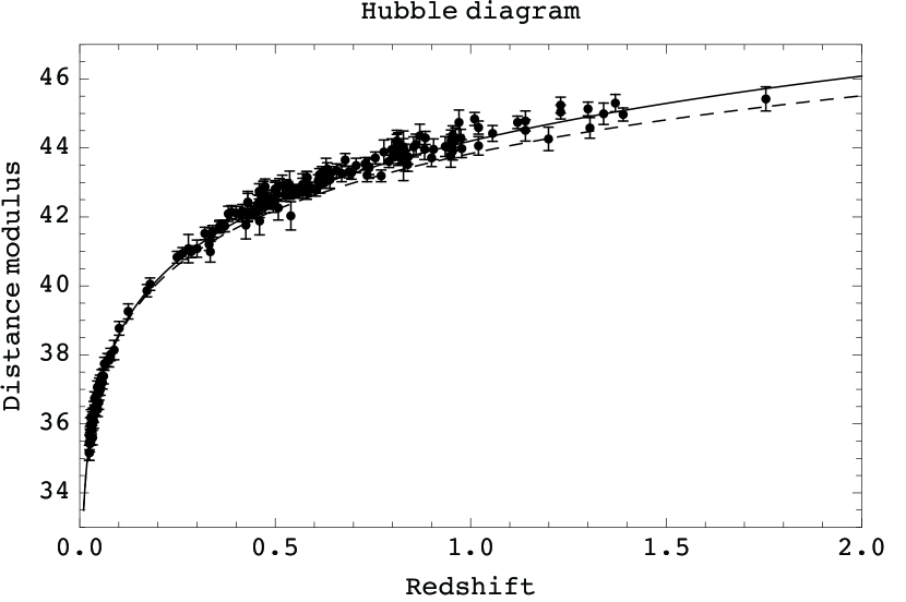
Figure 1: Hubble diagram fits for 182 high-confidence SNe Ia from Riess et al. (2007). The dashed line is a plot of Eq. 3 (flat universe with $m=0$), and the solid line is a plot of Eq. 9 ($m>0$). The horizontal axis is the redshift $z$, and the vertical axis is the photometrically determined distance modulus. The Hubble constant for each curve has been chosen to give the best fit to the observations.

In Fig. 1 we compare the most recent set of high-confidence (“gold”) (Riess et al., 2007) data for 182 SNe Ia sources distributed over the interval $0.0233\lesssim z\lesssim 1.755$ with two models in which $\Lambda=0$: GR for a flat universe, with $m=0$ (Eq. 3), and GR with $m>0$ (Eq. 9). The Hubble constant was determined by a weighted least-squares adjustment of the model to the data. For $m>0$, $H_{o}=60.1~{}\mathrm{km\;s}^{-1}\mathrm{\,Mpc}^{-1}(\chi^{2}=179)$, and for $m=0$, $H_{o}=55.4~{}\mathrm{km\;s}^{-1}\mathrm{\,Mpc}^{-1}(\chi^{2}=288)$. Because the number of degrees of freedom $\nu=180$ is large, $x=(\chi^{2}-\nu)/\sqrt{2\nu}$ is approximately normally distributed with unit variance (Cramér, 1958; Abramowitz & Stegun, 1964). For $m>0$, $x=-0.1$, whereas for $m=0$, $x=5.9$. The $m>0$ model is quite plausible, but the $m=0$ model is not; and the estimated $H_{o}$ for the $m>0$ model is appreciably closer to that of Riess et al. (1998) than is the estimate for $m=0$. Indeed, the $m>0$ model’s Hubble constant is even closer to the $H_{o}=62.3~{}\mathrm{km\;s}^{-1}\mathrm{\,Mpc}^{-1}$ estimate of Tammann, Sandage & Reindl (2008).

The Einstein-de Sitter ($m=0$) and Milne ($m>0$) models have power-law cosmologies in which the cosmological scale factor evolves as $a\propto t^{q}$. Assuming a power law parameterization, Sethi, Dev & Jain (2005) found the exponent that gives the best fit to the first 157 “gold” subset of SNe Ia data (Riess et al., 2004) is $q=1.04_{-0.06}^{+0.07}$. This provides additional support in favor of Milne’s model ($q=1$) over that of Einstein and de Sitter ($q=2/3$), but there are other cosmologies to consider, notably those involving dark matter and dark energy.

Table 1: Qualities of fit between the 182 “gold” supernovae for three cosmologies. All the calculations have been independently done for this paper. Where ${\mathchoice{\hbox{\raise 5.06941pt\hbox to0.0pt{\kern 1.45833pt\vrule width=2.91667pt,height=0.3pt,depth=0.3pt\hss}\hbox{$\displaystyle\lambda$}}}{\hbox{\raise 5.06941pt\hbox to0.0pt{\kern 1.45833pt\vrule width=2.91667pt,height=0.3pt,depth=0.3pt\hss}\hbox{$\textstyle\lambda$}}}{\hbox{\raise 3.54857pt\hbox to0.0pt{\kern 1.02083pt\vrule width=2.04167pt,height=0.3pt,depth=0.3pt\hss}\hbox{$\scriptstyle\lambda$}}}{\hbox{\raise 2.5347pt\hbox to0.0pt{\kern 0.72916pt\vrule width=1.45833pt,height=0.3pt,depth=0.3pt\hss}\hbox{$\scriptscriptstyle\lambda$}}}}\ll c/H_{o}=L_{H}$ (the Hubble length), the $m>0$ model is equivalent to a Milne universe. The conventional cosmological parameters, $\Omega_{m},\,\Omega_{\Lambda},\,\mathrm{and}\;\Omega_{R}$, are associated with the density, the cosmological constant, and the curvature; and $h$ is the Hubble parameter.

Universe	$\Omega_{m}$	$\Omega_{\Lambda}$	$\Omega_{R}$	$h$	$\chi^{2}$	$x$
$\Lambda$CDM	0.29	0.71	0.00	0.647	164	-0.8
Einstein-de Sitter	1.00	0.00	0.00	0.554	288	+5.7
Milne	0.00	0.00	1.00	0.601	179	-0.1

Riess et al. (2007) proffered the $\Lambda$CDM model with cold dark matter and dark energy ($\Omega_{m}=0.29,\Omega_{\Lambda}=0.71$), fitting their “gold” data set with $\chi^{2}=150$, which is appreciably less than our Milne fit’s $\chi^{2}=179$. However, their Milne fit’s $\chi^{2}=164$ is also less than ours; yet they fit the Einstein-de Sitter model, with $\chi^{2}=285$, which is close to our $\chi^{2}=288$. Our calculations differed somewhat from theirs, and we could discern no pattern to the offsets, so we recalculated their $\Lambda$CDM model fit, and found $\chi^{2}=164$, and $x=-0.8$. Our fits to the $\Lambda$CDM, Einstein-de Sitter, and Milne models are summarized in Table 1. The Hubble parameter, $h=H_{o}/(100\,\mathrm{km\;s}^{-1}\mathrm{\,Mpc}^{-1})$, is the only free parameter for each fit. The results are independent of the two fitting technique we used - marginalization and conventional weighted least-squares. Our $h$ estimates are valid only if there are no systematic uncertainties, including that of the SN Ia absolute magnitude. As an example of the sensitivity, a systematic uncertainty of $\pm 0.03$ mag (Hicken et al., 2009) would cause $h$ to be offset by $\mp 0.0083$. Even so, the systematic uncertainties affect only the $h$ estimates, but not the $\chi^{2}$ results.

If the criterion for the better fit is having the lower $\chi^{2}$, then the $\Lambda$CDM model ($\chi^{2}=164$) clearly edges the Milne model ($\chi^{2}=179$). However, if we give full credence to the observation variances (that is, if we assume that they are not exaggerated), then the criterion for the better fit is having the higher likelihood. The maximum likelihood is at the peak of the $x$ normal distribution, $x=0$, so then the Milne model ($x=-0.1$) edges the $\Lambda$CDM model ($x=-0.8$), but this comparison is for solutions that minimize $\chi^{2}$ rather than minimize $x$. In both cases $x<0$, so by varying the solution parameters from the least-squares determinations, $x$ will increase from its minimum, and there will be non-unique solutions for which $x=0$. For example, the only parameter for the $m>0$ model is $h$, and the two roots to $x(h)=0$ are $h=0.596$ and $h=0.607$. With three independent parameters ($h,\,\Omega_{m},\,\Omega_{\Lambda}$), the $\Lambda$CDM model is more complicated because it involves a hypersurface rather than a curve. By varying each parameter, one at a time, from the $\chi^{2}$ minimum, six solutions for $x=0$ can (in principle) be found; but if they are all allowed to vary together, then there will be a continuum of solutions. The relative plausibility of these two models cannot be definitively settled by statistics. We prefer instead to invoke Occam’s razor: (1) the $\Lambda$CDM model requires cosmological attractions by vast amounts of dark matter that are largely countered by cosmological repulsions by vast amounts of dark energy, whereas (2) the $m>0$ model merely requires that the graviton not be massless. Occam’s razor favors the second. Moreover, by not requiring a $\Lambda$ term, we avoid conceptual difficulties, such as those described by Carroll (2001), who considers a non-zero $\Lambda$ to be exceedingly problematic, but who also concedes that denying its existence in face of GR and existing data is even more problematic. The massive graviton alternative has the additional advantage that it is not sensitive to the graviton mass, provided only that $m$ is not identically zero. Finally, if there are no massless gravitons, then there is no critical density below which the universe is open; the universe is necessarily open.

4 The graviton mass

Although the results in Fig. 1 are insensitive to the specific value of $m$ provided that $m\not=0$, it is interesting to consider the limits on $m$ that do exist. Following Will (2001) we assume that in the absence of other long range forces, the effect of a massive graviton is to replace the Newtonian gravitational potential $-GM/r$ of a point mass $M$ by the Yukawa potential $-(GM/r)e^{-r/{\mathchoice{\hbox{\raise 3.54857pt\hbox to0.0pt{\kern 1.02083pt\vrule width=2.04167pt,height=0.3pt,depth=0.3pt\hss}\hbox{$\displaystyle\lambda$}}}{\hbox{\raise 3.54857pt\hbox to0.0pt{\kern 1.02083pt\vrule width=2.04167pt,height=0.3pt,depth=0.3pt\hss}\hbox{$\textstyle\lambda$}}}{\hbox{\raise 2.484pt\hbox to0.0pt{\kern 0.71458pt\vrule width=1.42917pt,height=0.3pt,depth=0.3pt\hss}\hbox{$\scriptstyle\lambda$}}}{\hbox{\raise 1.77428pt\hbox to0.0pt{\kern 0.5104pt\vrule width=1.02083pt,height=0.3pt,depth=0.3pt\hss}\hbox{$\scriptscriptstyle\lambda$}}}}}$. Hence any system of characteristic size $R$ whose behavior is correctly described by Newtonian gravity implies a limit ${\mathchoice{\hbox{\raise 5.06941pt\hbox to0.0pt{\kern 1.45833pt\vrule width=2.91667pt,height=0.3pt,depth=0.3pt\hss}\hbox{$\displaystyle\lambda$}}}{\hbox{\raise 5.06941pt\hbox to0.0pt{\kern 1.45833pt\vrule width=2.91667pt,height=0.3pt,depth=0.3pt\hss}\hbox{$\textstyle\lambda$}}}{\hbox{\raise 3.54857pt\hbox to0.0pt{\kern 1.02083pt\vrule width=2.04167pt,height=0.3pt,depth=0.3pt\hss}\hbox{$\scriptstyle\lambda$}}}{\hbox{\raise 2.5347pt\hbox to0.0pt{\kern 0.72916pt\vrule width=1.45833pt,height=0.3pt,depth=0.3pt\hss}\hbox{$\scriptscriptstyle\lambda$}}}}\gtrsim R$. Several authors (Will, 2001, 1998; Goldhaber & Nieto, 1974; Visser, 1998) have analyzed data for various astrophysical systems to set limits on  $\textstyle\lambda$. Using solar system data from Talmadge et al. (1988), Will finds ${\mathchoice{\hbox{\raise 5.06941pt\hbox to0.0pt{\kern 1.45833pt\vrule width=2.91667pt,height=0.3pt,depth=0.3pt\hss}\hbox{$\displaystyle\lambda$}}}{\hbox{\raise 5.06941pt\hbox to0.0pt{\kern 1.45833pt\vrule width=2.91667pt,height=0.3pt,depth=0.3pt\hss}\hbox{$\textstyle\lambda$}}}{\hbox{\raise 3.54857pt\hbox to0.0pt{\kern 1.02083pt\vrule width=2.04167pt,height=0.3pt,depth=0.3pt\hss}\hbox{$\scriptstyle\lambda$}}}{\hbox{\raise 2.5347pt\hbox to0.0pt{\kern 0.72916pt\vrule width=1.45833pt,height=0.3pt,depth=0.3pt\hss}\hbox{$\scriptscriptstyle\lambda$}}}}>2.8\times 10^{12}$ km, and from galaxy supercluster data one can infer ${\mathchoice{\hbox{\raise 5.06941pt\hbox to0.0pt{\kern 1.45833pt\vrule width=2.91667pt,height=0.3pt,depth=0.3pt\hss}\hbox{$\displaystyle\lambda$}}}{\hbox{\raise 5.06941pt\hbox to0.0pt{\kern 1.45833pt\vrule width=2.91667pt,height=0.3pt,depth=0.3pt\hss}\hbox{$\textstyle\lambda$}}}{\hbox{\raise 3.54857pt\hbox to0.0pt{\kern 1.02083pt\vrule width=2.04167pt,height=0.3pt,depth=0.3pt\hss}\hbox{$\scriptstyle\lambda$}}}{\hbox{\raise 2.5347pt\hbox to0.0pt{\kern 0.72916pt\vrule width=1.45833pt,height=0.3pt,depth=0.3pt\hss}\hbox{$\scriptscriptstyle\lambda$}}}}\gtrsim 6\times 10^{19}$ km (Will, 2001, 1998; Goldhaber & Nieto, 1974; Visser, 1998). Other lower limits on  $\textstyle\lambda$ are summarized in Will (2001). Utilizing the previous arguments we can infer an upper limit for  $\textstyle\lambda$. Suppose that there is an immense volume of uniform density matter whose extent is many skin depths ( $\textstyle\lambda$’s). On a point mass that is several skin depths inside the outer surface of the volume, the specific force due to the Yukawa potential is zero, since the source appears the same in all directions. Suppose next that this volume is divided into two parts: one is a sphere of radius $r\ll$  $\textstyle\lambda$, and the other part is the remainder of the volume with the sphere removed. The sphere is the source of a force directed toward its center (which can easily be quantified), so the remainder of the volume is the source of a force of an identical magnitude, but directed away from the center of the sphere. Hence if there exists a vast uniform density volume, and somewhere deep inside it there is a density perturbation that makes the local density smaller than the mean density, then the lower density matter will be accelerated outward. At the outer boundary of the volume matter will, of course, be accelerated inwards. The volume will transform toward being a hollow bubble until the thickness of the higher density bubble matter is just a few skin depths. There are some additional considerations: conservation of angular momentum places a constraint on how far the inward moving matter can progress although it does not, by itself, constrain how far the outward moving matter can go. According to Dolgov, Sazhin & Zeldovich (1990), “clusters of galaxies form surfaces with a thickness of about 10-20 Mpc surrounding empty regions with characteristic size of 100-200 Mpc.” With the estimate

$${\mathchoice{\hbox{\raise 5.06941pt\hbox to0.0pt{\kern 1.45833pt\vrule width=2.91667pt,height=0.3pt,depth=0.3pt\hss}\hbox{$\displaystyle\lambda$}}}{\hbox{\raise 5.06941pt\hbox to0.0pt{\kern 1.45833pt\vrule width=2.91667pt,height=0.3pt,depth=0.3pt\hss}\hbox{$\textstyle\lambda$}}}{\hbox{\raise 3.54857pt\hbox to0.0pt{\kern 1.02083pt\vrule width=2.04167pt,height=0.3pt,depth=0.3pt\hss}\hbox{$\scriptstyle\lambda$}}}{\hbox{\raise 2.5347pt\hbox to0.0pt{\kern 0.72916pt\vrule width=1.45833pt,height=0.3pt,depth=0.3pt\hss}\hbox{$\scriptscriptstyle\lambda$}}}}\approx 5\,\mathrm{Mpc},$$ (11)

the gravitational force is significant for galaxy superclusters and also between neighboring superclusters that form a “surface,” but negligible in the vast empty regions between the surfaces. A skin depth ${\mathchoice{\hbox{\raise 5.06941pt\hbox to0.0pt{\kern 1.45833pt\vrule width=2.91667pt,height=0.3pt,depth=0.3pt\hss}\hbox{$\displaystyle\lambda$}}}{\hbox{\raise 5.06941pt\hbox to0.0pt{\kern 1.45833pt\vrule width=2.91667pt,height=0.3pt,depth=0.3pt\hss}\hbox{$\textstyle\lambda$}}}{\hbox{\raise 3.54857pt\hbox to0.0pt{\kern 1.02083pt\vrule width=2.04167pt,height=0.3pt,depth=0.3pt\hss}\hbox{$\scriptstyle\lambda$}}}{\hbox{\raise 2.5347pt\hbox to0.0pt{\kern 0.72916pt\vrule width=1.45833pt,height=0.3pt,depth=0.3pt\hss}\hbox{$\scriptscriptstyle\lambda$}}}}=5$ Mpc $=1.6\times 10^{20}$ km corresponds to $m=1.3\times 10^{-30}$ eV$/c^{2}$; hence we conjecture that $m\sim 10^{-30}$ eV$/c^{2}$. It is then conceivable that there could be heavier gravitons in addition to this lightest graviton, with masses somewhere in the range

$$1.3\times 10^{-30}\mbox{ eV}/c^{2}<m<7.4\times 10^{-23}\mbox{ eV}/c^{2},$$ (12)

which corresponds to

$$1.6\times 10^{20}\mathrm{\,km}>\mathrm{{\mathchoice{\hbox{\raise 5.06941pt\hbox to0.0pt{\kern 1.45833pt\vrule width=2.91667pt,height=0.3pt,depth=0.3pt\hss}\hbox{$\displaystyle\lambda$}}}{\hbox{\raise 5.06941pt\hbox to0.0pt{\kern 1.45833pt\vrule width=2.91667pt,height=0.3pt,depth=0.3pt\hss}\hbox{$\textstyle\lambda$}}}{\hbox{\raise 3.54857pt\hbox to0.0pt{\kern 1.02083pt\vrule width=2.04167pt,height=0.3pt,depth=0.3pt\hss}\hbox{$\scriptstyle\lambda$}}}{\hbox{\raise 2.5347pt\hbox to0.0pt{\kern 0.72916pt\vrule width=1.45833pt,height=0.3pt,depth=0.3pt\hss}\hbox{$\scriptscriptstyle\lambda$}}}}}>2.8\times 10^{12}\mathrm{\,km}.$$ (13)

The Laser Interferometer Space Antenna (LISA) gravitational wave detector would not be able to detect the $m\sim 10^{-30}$ eV$/c^{2}$ mass, but it might be sensitive to the more massive gravitons in the range of Eq. 12 if, indeed, any exist (Will, 1998).

5 The cosmic microwave background (CMB)

If $m>0$, the dynamics of a baryon fluid at the epoch of recombination differ substantially from those of conventional models which tacitly assume that the graviton is massless. In Section 4, we explained why a massive body with dimensions that are large compared with  $\textstyle\lambda$ would not be stable, but instead would tend to separate into smaller bodies with dimensions that are of the order of a few skin depths or less - that is, to the the scale of galaxy superclusters. We hypothesize that this instability is the principal cause of CMB power spectrum anisotropies. On recombination, massive bodies with breadths larger than, say, $D=4{\mathchoice{\hbox{\raise 5.06941pt\hbox to0.0pt{\kern 1.45833pt\vrule width=2.91667pt,height=0.3pt,depth=0.3pt\hss}\hbox{$\displaystyle\lambda$}}}{\hbox{\raise 5.06941pt\hbox to0.0pt{\kern 1.45833pt\vrule width=2.91667pt,height=0.3pt,depth=0.3pt\hss}\hbox{$\textstyle\lambda$}}}{\hbox{\raise 3.54857pt\hbox to0.0pt{\kern 1.02083pt\vrule width=2.04167pt,height=0.3pt,depth=0.3pt\hss}\hbox{$\scriptstyle\lambda$}}}{\hbox{\raise 2.5347pt\hbox to0.0pt{\kern 0.72916pt\vrule width=1.45833pt,height=0.3pt,depth=0.3pt\hss}\hbox{$\scriptscriptstyle\lambda$}}}}$ (that is, with radii exceeding two skin depths if the bodies are spheres) would divide into lesser sized bodies separated from each other by the distance of approximately $D$. Because the universe has expanded, the nominal separation distance of observed radiation peaks from the last scattering surface, with redshift $z_{\star}$, is $(1+z_{\star})D$; and the nominal angular separation of peaks on the celestial sphere for $z_{\star}^{2}\gg 1$ is (see Eq. 10)

$$\gamma=\frac{(1+z_{\star})D}{a_{o}f}\approx\frac{2H_{o}D}{c}=\frac{8{\mathchoice{\hbox{\raise 5.06941pt\hbox to0.0pt{\kern 1.45833pt\vrule width=2.91667pt,height=0.3pt,depth=0.3pt\hss}\hbox{$\displaystyle\lambda$}}}{\hbox{\raise 5.06941pt\hbox to0.0pt{\kern 1.45833pt\vrule width=2.91667pt,height=0.3pt,depth=0.3pt\hss}\hbox{$\textstyle\lambda$}}}{\hbox{\raise 3.54857pt\hbox to0.0pt{\kern 1.02083pt\vrule width=2.04167pt,height=0.3pt,depth=0.3pt\hss}\hbox{$\scriptstyle\lambda$}}}{\hbox{\raise 2.5347pt\hbox to0.0pt{\kern 0.72916pt\vrule width=1.45833pt,height=0.3pt,depth=0.3pt\hss}\hbox{$\scriptscriptstyle\lambda$}}}}}{L_{H}},$$ (14)

where $L_{H}=c/H_{o}$ is the Hubble length. Setting $h=0.60$ (from Table 1) and ${\mathchoice{\hbox{\raise 5.06941pt\hbox to0.0pt{\kern 1.45833pt\vrule width=2.91667pt,height=0.3pt,depth=0.3pt\hss}\hbox{$\displaystyle\lambda$}}}{\hbox{\raise 5.06941pt\hbox to0.0pt{\kern 1.45833pt\vrule width=2.91667pt,height=0.3pt,depth=0.3pt\hss}\hbox{$\textstyle\lambda$}}}{\hbox{\raise 3.54857pt\hbox to0.0pt{\kern 1.02083pt\vrule width=2.04167pt,height=0.3pt,depth=0.3pt\hss}\hbox{$\scriptstyle\lambda$}}}{\hbox{\raise 2.5347pt\hbox to0.0pt{\kern 0.72916pt\vrule width=1.45833pt,height=0.3pt,depth=0.3pt\hss}\hbox{$\scriptscriptstyle\lambda$}}}}\approx 5$ Mpc (Eq. 11), we calculate $\gamma\approx 0.008\,\mathrm{radians}\approx 0.5^{\circ}$, which is close to what has been observed (Lange et al., 2001; Spergel et al., 2003).

6 Summary

Massive gravitons lead to an alternative relation between the luminosity distance [$a_{o}r$ versus $a_{o}f_{o}$ from Eq. 10] and the redshift $z$ [Eq. 9 versus Eq. 3]. A comparison of Eqs. 9 and 3 in the framework of a cosmology with $\Lambda=0$ favors the massive graviton alternative, as discussed in the text and shown in Fig. 1. Moreover, our graviton mass estimate, $m\sim 10^{-30}$ eV$/c^{2}$, is consistent with the structure of galaxy superclusters and with the pattern of the cosmic microwave background. Although the redshift data could be attributable to a $\Lambda$CDM model (Riess et al., 2004), doing so would conflict with the rule of thumb that “less is better” because of the need for additional suppositions.

7 Conclusions

The inverse-square law is the only possible law that leads to a cosmological contracting acceleration. Its GR heritage, common acceptance, usage and applicability over broad but limited domain lead us to consider it to be the norm. It need not be; indeed we might even consider it to be a peculiar exception.

Any force law that assigns the graviton a mass, $m>0$, is a local law because the force falls off both geometrically (like the inverse-square law) and exponentially with distance. In that case, the cosmological principle that “everything is the same everywhere” is not even needed. A weaker principle would suffice, for example the cosmological legal principle that “every physical law is the same everywhere.” Gravity pulls the clusters in a supercluster together, but it does not pull distinct superclusters together. The gravity-free Milne model is underlain by local gravity effects that lead to our interesting universe rather than a featureless cloud of expanding matter. Dark matter and dark energy are then regarded as gratuitous Procrustean artifacts.

Appendix A Contrasting the Newtonian and Yukawa Accelerations in a Uniform Density Universe

We contrast the familiar Newtonian acceleration with the less familiar Yukawa acceleration, starting with a model for which there is only a thin spherical shell of mass $dM$ at $r=a$.

A.1 Newtonian Potential Inside the Shell

The Newtonian potential $d\Psi_{N}(r,a)$ at the origin is $d\Psi_{N}(0,a)=-G\,dM/a$, and the Newtonian potential satisfies the homogeneous equation $\nabla^{2}d\Psi_{N}=0$ (in free space), whose solution is a linear combination of $d\Psi_{N}=\mathrm{constant}$ and $d\Psi_{N}\propto 1/r$. The only such solution that satisfies $d\Psi_{N}(0,a)=-G\,dM/a$ is

$$d\Psi_{N}(r,a)=-G\,dM/a,\;r\leq a.$$ (15)

The solution interval is closed at the shell because the potential (but not its gradient) is continuous there. The potential has no gradient for $r<a$, so there is no Newtonian gravitational acceleration inside the shell. This is Newton’s “iron sphere theorem” (Peebles, 1993).

A.2 Yukawa Potential Inside the Shell

The Yukawa potential at the origin is $d\Psi_{Y}(0,a)=-G\,dM\exp(-\mu a)/a$. The Yukawa potential in free space satisfies the homogeneous equation $\nabla^{2}d\Psi_{Y}-\mu^{2}d\Psi_{Y}=0$, whose solutions are linear combinations of $\exp(\pm\mu r)/r$. The only such combination that equals $d\Psi_{Y}(0,a)$ at the origin is $d\Psi_{Y}(0,a)\sinh(\mu r)/(\mu r)$, so the Yukawa potential inside and on the shell is

$$d\Psi_{Y}(r,a)=-G\,dM\,\frac{\exp(-\mu a)}{a}\;\frac{\sinh(\mu r)}{\mu r}\equiv\frac{\partial w_{1}(r,a)}{\partial a}\,da,\;r\leq a.$$ (16)

A.3 Newtonian Potential Outside the Shell

The solution to $\nabla^{2}d\Psi_{N}=0$ that equals $d\Psi_{N}(a,a)$ at $r=a$ and approaches zero as $r\rightarrow\infty$ is

$$d\Psi_{N}(r,a)=-G\,dM/r,\;r\geq a.$$ (17)

Outside the shell, the Newtonian gravitational acceleration (the gradient of the potential), follows the inverse square law.

A.4 Yukawa Potential Outside the Shell

The solution to $\nabla^{2}d\Psi_{Y}-\mu^{2}d\Psi_{Y}=0$ that equals $f_{1}(a,a)$ at $r=a$ and remains finite outside the shell is

$$d\Psi_{Y}(r,a)=-G\,dM\,\frac{\sinh(\mu a)}{\mu a}\;\frac{\exp(-\mu r)}{r}\equiv\frac{\partial w_{2}(r,a)}{\partial a}\,da,\;r\geq a.$$ (18)

Note that $\partial w_{1}(r,a)/\partial a=\partial w_{2}(a,r)/\partial a$.

We next integrate over $a$ to derive the Newtonian and Yukawa gravitational potentials in a uniform density universe, for which $dM=4\pi\rho a^{2}\,da$. For $\Psi_{N}$, this is a trivial exercise.The integral of Eq . 17 is $-GM/r\propto-r^{2}$, where $M$ is the mass of the sphere $r\leq a$; this is the familiar Newtonian gravitational potential. The integral of Eq. 15 is $-G(M_{U}-M)/a$, where $M_{U}$ is the mass of the universe inside the cosmic horizon. The radial gradient of the Newtonian potential is $GM/r^{2}$; at $r=a$, it proportional to $a$, so there is a gravitational attraction between any two points that is proportional to their separation distance. If $m=0$, the universe has a uniform contracting gravitational acceleration.

A.5 Derivation of Eq. 5

The integral of Eq. 16 is

$$W_{1}(r)=\int_{r}^{\infty}\frac{\partial w_{1}(r,a)}{\partial a}\,da=-4\pi G\rho{\mathchoice{\hbox{\raise 5.06941pt\hbox to0.0pt{\kern 1.45833pt\vrule width=2.91667pt,height=0.3pt,depth=0.3pt\hss}\hbox{$\displaystyle\lambda$}}}{\hbox{\raise 5.06941pt\hbox to0.0pt{\kern 1.45833pt\vrule width=2.91667pt,height=0.3pt,depth=0.3pt\hss}\hbox{$\textstyle\lambda$}}}{\hbox{\raise 3.54857pt\hbox to0.0pt{\kern 1.02083pt\vrule width=2.04167pt,height=0.3pt,depth=0.3pt\hss}\hbox{$\scriptstyle\lambda$}}}{\hbox{\raise 2.5347pt\hbox to0.0pt{\kern 0.72916pt\vrule width=1.45833pt,height=0.3pt,depth=0.3pt\hss}\hbox{$\scriptscriptstyle\lambda$}}}}^{2}\,\frac{\exp(-\mu r)(1+\mu r)\sinh(\mu r)}{\mu r},$$ (19)

and the integral of Eq. 18 is

$$W_{2}(r)=\int_{0}^{r}\frac{\partial w_{2}(r,a)}{\partial a}\,da=-4\pi G\rho{\mathchoice{\hbox{\raise 5.06941pt\hbox to0.0pt{\kern 1.45833pt\vrule width=2.91667pt,height=0.3pt,depth=0.3pt\hss}\hbox{$\displaystyle\lambda$}}}{\hbox{\raise 5.06941pt\hbox to0.0pt{\kern 1.45833pt\vrule width=2.91667pt,height=0.3pt,depth=0.3pt\hss}\hbox{$\textstyle\lambda$}}}{\hbox{\raise 3.54857pt\hbox to0.0pt{\kern 1.02083pt\vrule width=2.04167pt,height=0.3pt,depth=0.3pt\hss}\hbox{$\scriptstyle\lambda$}}}{\hbox{\raise 2.5347pt\hbox to0.0pt{\kern 0.72916pt\vrule width=1.45833pt,height=0.3pt,depth=0.3pt\hss}\hbox{$\scriptscriptstyle\lambda$}}}}^{2}\,\frac{\exp(-\mu r)[\mu r\cosh(\mu r)-\sinh(\mu r)]}{\mu r}.$$ (20)

Their sum is $W_{1}(r)+W_{2}(r)=-4\pi G\rho{\mathchoice{\hbox{\raise 5.06941pt\hbox to0.0pt{\kern 1.45833pt\vrule width=2.91667pt,height=0.3pt,depth=0.3pt\hss}\hbox{$\displaystyle\lambda$}}}{\hbox{\raise 5.06941pt\hbox to0.0pt{\kern 1.45833pt\vrule width=2.91667pt,height=0.3pt,depth=0.3pt\hss}\hbox{$\textstyle\lambda$}}}{\hbox{\raise 3.54857pt\hbox to0.0pt{\kern 1.02083pt\vrule width=2.04167pt,height=0.3pt,depth=0.3pt\hss}\hbox{$\scriptstyle\lambda$}}}{\hbox{\raise 2.5347pt\hbox to0.0pt{\kern 0.72916pt\vrule width=1.45833pt,height=0.3pt,depth=0.3pt\hss}\hbox{$\scriptscriptstyle\lambda$}}}}^{2}=-3GM_{{\mathchoice{\hbox{\raise 3.54857pt\hbox to0.0pt{\kern 1.02083pt\vrule width=2.04167pt,height=0.3pt,depth=0.3pt\hss}\hbox{$\displaystyle\lambda$}}}{\hbox{\raise 3.54857pt\hbox to0.0pt{\kern 1.02083pt\vrule width=2.04167pt,height=0.3pt,depth=0.3pt\hss}\hbox{$\textstyle\lambda$}}}{\hbox{\raise 2.484pt\hbox to0.0pt{\kern 0.71458pt\vrule width=1.42917pt,height=0.3pt,depth=0.3pt\hss}\hbox{$\scriptstyle\lambda$}}}{\hbox{\raise 1.77428pt\hbox to0.0pt{\kern 0.5104pt\vrule width=1.02083pt,height=0.3pt,depth=0.3pt\hss}\hbox{$\scriptscriptstyle\lambda$}}}}}/{\mathchoice{\hbox{\raise 5.06941pt\hbox to0.0pt{\kern 1.45833pt\vrule width=2.91667pt,height=0.3pt,depth=0.3pt\hss}\hbox{$\displaystyle\lambda$}}}{\hbox{\raise 5.06941pt\hbox to0.0pt{\kern 1.45833pt\vrule width=2.91667pt,height=0.3pt,depth=0.3pt\hss}\hbox{$\textstyle\lambda$}}}{\hbox{\raise 3.54857pt\hbox to0.0pt{\kern 1.02083pt\vrule width=2.04167pt,height=0.3pt,depth=0.3pt\hss}\hbox{$\scriptstyle\lambda$}}}{\hbox{\raise 2.5347pt\hbox to0.0pt{\kern 0.72916pt\vrule width=1.45833pt,height=0.3pt,depth=0.3pt\hss}\hbox{$\scriptscriptstyle\lambda$}}}}$, the same as Eq. 5. If $m>0$, the universe has no gravitational acceleration.

If we let $\mu\rightarrow 0$ in Eqs. 16 and 18, then they become Eqs. 15 and 17; there is no $m=0$ discontinuity for thin shells. However, if we first integrate over all shells, then $\Psi_{Y}$ is independent of $r$, whereas $\Psi_{N}\propto 1/r$; letting $\mu\rightarrow 0$ after the integration does not change this situation.

Appendix B Derivation of the Metric

We used Leonard Parker’s Mathematica (Wolfram, 1999) notebook, Curvature and the Einstein Equation (Hartle, 2002), to determine $f(r)$ in the Eq. 1 metric, when the distance formula is Eq. 6. The only change we made to the notebook was in the definition of the metric, using these two statements:

a=a0+adot t

metric={{-a^∧2,0,0,0},{0,-(a f[r])^∧2,0,0},{0,0,-(a f[r])^∧2 Sin[$\theta$]^∧2,0},{0,0,0,c^∧2}}.

Then the $G_{22}$ ($G_{\theta\theta}$) component of the Einstein tensor turned out to be

$$G_{22}=f(r)\left[f^{\prime\prime}(r)-(\dot{a}/c)^{2}\right].$$ (21)

Eq. 7 is an evident solution to $G_{22}=0$, so we substituted it back into the Mathematica notebook by defining

f[r]=(c/adot) Sinh[adot r/c],

and all components of the Einstein tensor turned out to be zero. QED.

Appendix C Acknowledgements

We thank the referee for several helpful comments.

The work of EF was supported in part by the U.S. Department of Energy under Contract No. DE-AC02-76ER071428.

References

• Abramowitz & Stegun (1964) Abramowitz, M., & Stegun, I. A., 1964, Handbook of Mathematical Functions (Washington, DC: National Bureau of Standards)
• Arun & Will (2009) Arun, K. G., & Will, C. M. 2009, Class. Quantum Grav. 26 (2009) 155002
• Carroll (2001) Carroll, S. M. 2001, Living Rev. Relativity 4, 1
• Cramér (1958) Cramér, H. 1958, Mathematical Methods of Statistics (Princeton: Princeton University Press)
• Creminelli et al. (2005) Creminelli, P., Nicolis, A., Papucci, M., & Trincherini, E. 2005, J. High Energy Phys. 9, 3
• Deffayet et al. (2002) Deffayet, C., Dvali, G., Gabadadze, G., & Vainstein, A. 2002, Phys.Rev. D 65, 044026
• Deffayet & Rombouts (2005) Deffayet, C., & Rombouts, J. W. 2005, Phys. Rev. D 72, 044003
• Dolgov, Sazhin & Zeldovich (1990) Dolgov, A. D., Sazhin, M. V., & Zeldovich, Ya. B. 1990, Basics of Modern Cosmology (Gif-sur-Yvette: Editions Frontières)
• Gabadadze & Gruzinov (2005) Gabadadze, G., & Gruzinov, A. 2005, Phys. Rev. D 72, 124007
• Goldhaber & Nieto (2009) Goldhaber, A. S., & Nieto, M. M. 2009, Rev. Mod. Phys. in press
• Goldhaber & Nieto (1974) Goldhaber, A. S., & Nieto, M. M. 1974, Phys. Rev. D 9, 1119
• Gruzinov (2005) Gruzinov, A. 2005, New Astron. 10, 311
• Hartle (2002) Hartle, J. B. 2002, Gravity: An Introduction to Einstein’s General Relativity (Boston: Addison-Wesley Pub Co.)
• Hicken et al. (2009) Hicken, M., et al. 2009, ApJ accepted
• Lange et al. (2001) Lange, A. E., et al. 2001, Phys.Rev. D 63, 042001
• Maggiore (2008) Maggiore, M. 2008, Gravitational Waves (Oxford: Oxford University Press)
• Peebles (1993) Peebles, P. J. E. 1993, Principles of Physical Cosmology (Princeton: Princeton University Press)
• Perlmutter et al. (1999) Perlmutter, S., et al. 1999, ApJ 517, 565
• Riess et al. (1998) Riess, A. G., et al. 1998, AJ 116, 1009
• Riess et al. (2004) Riess, A. G., et al. 2004, ApJ 607, 665
• Riess et al. (2007) Riess, A. G., et al. 2007, ApJ 659, 98
• Sethi, Dev & Jain (2005) Sethi, G., Dev, A., & Jain, D. 2005, Phys. Lett. B 624, 135
• Spergel et al. (2003) Spergel, D. N., et al. 2003, ApJS 148, 175
• Talmadge et al. (1988) Talmadge, C., Berthias, J.-P., Hellings, R. W., & Standish, E. M. 1988, Phys. Rev. Lett. 61, 1159
• Tammann, Sandage & Reindl (2008) Tammann, G. A., Sandage, A., & Reindl, B. 2008, AAR 15, 289
• Vainshtein (1972) Vainshtein, A. I. 1972, Phys. Lett. B 39, 393
• van Dam & Veltman (1970) van Dam, H., & Veltman, M. 1970, Nucl. Phys. B 22, 397
• Visser (1998) Visser, M. 1998, Gen. Relativ. Gravit. 30, 1717
• Will (1998) Will, C. M. 1998, Phys. Rev. D 57, 2061
• Will (2001) Will, C. M. 2001, Living Rev. Relativity 4, 4
• Wolfram (1999) Wolfram, S. 1999, The Mathematica Book (Wolfram Media/Cambridge University Press)
• Zakharov (1970) Zakharov, V. I. 1970, JETP Lett. 12, 312
• Zee (2003) Zee, A. 2003, Quantum Field Theory in a Nutshell (Princeton University Press)